Impact Force of a Geomorphic Dam-Break Wave against an Obstacle: Effects of Sediment Inertia

Abstract

The evaluation of the impact force on structures due to a flood wave is of utmost importance for estimating physical damage and designing adequate countermeasures. The present study investigates, using 2D shallow-water approximation, the morphodynamics and forces caused by a dam-break wave against a rigid obstacle in the presence of an erodible bed. A widely used coupled equilibrium model, based on the two-dimensional Saint–Venant hydrodynamic equations combined with the sediment continuity Exner equation (SVEM), is compared with a more complex two-phase model (TPM). Considering an experimental set-up presented in the literature with a single rigid obstacle in a channel, two series of tests were performed, assuming sand or light sediments on the bottom. The former test is representative of a typical laboratory experiment, and the latter may be scaled up to a field case. For each test, two different particle diameters were considered. Independently from the particle size, it was found that in the sand tests, SVEM performs similarly to TPM. In the case of light sediment, larger differences are observed, and the SVEM predicts a higher force of about 26% for both considered diameters. The analysis of the flow fields and the morphodynamics shows these differences can be essentially ascribed to the role of inertia of the solid particles.

1. Introduction

In many mountainous regions of the world, human settlements have developed in time, privileging torrential fans [1,2]. However, these areas may be exposed to important environmental risks due to extreme floods, during which flows with non-negligible sediment transport, such as those triggered by heavy rainfall or snow melting, may develop and cause intense erosion, deposition and remobilization processes [3,4,5]. The magnitude of these flows is nowadays impressively increasing due to climate change [6,7]. Moreover, the flood impact on a variety of obstacles, such as residential, commercial or industrial buildings or infrastructures, is responsible for dramatic consequences [8]. Therefore, a correct evaluation of the impact force is very important for estimating structural damage and designing protective countermeasures.

The presence of an erodible bed adds to the complexity of the phenomenon since the sediment transport influences the wave propagation and the impact force. Moreover, the morphological changes induced by the flow may expose the obstacle to unexpected loading conditions, contributing to its structural damage. From a modeling point of view, the study of the complex interaction between the sediment-laden flow and obstacles on erodible beds, essential in evaluating hazard levels and supporting the design of structural countermeasures, requires the prediction of both hydro and sediment dynamics [9].

Most of the attempts to assess torrential hazards rely on the use of empirical correlations between the estimated impact forces and the expected degree of damage for individual buildings [10,11,12,13,14]. However, similar approaches suffer from being extremely site-specific and difficult to generalize. For the sake of a more general and scalable approach, the simulation models represent a valid alternative [5]. Moreover, the presence of structures, along with the topography complexity, imposes the use of 2D or 3D models. Although in several cases the three-dimensional effects are not negligible, 2D shallow-water models, i.e., depth-averaged models, are widely accepted for most engineering applications. For instance, in the presence of non-erodible beds and rigid obstacles, Shige-eda and Akiyama [15] experimentally and numerically investigated the behavior of two-dimensional (2D) flood flows and the hydrodynamic force acting on structures. It has been shown that hydrodynamics and the force on structures may be predicted with enough accuracy through a shallow-water model. Bukreev [16] confirmed the applicability of the shallow-water approach to evaluate the dynamic action of a dam-break wave exerted on a vertical wall. Soares-Frazao and Zech [17], comparing the numerical results with experimental data, showed the ability of a 2D numerical model in reproducing the propagation of a dam-break wave in an idealized urban area. The potentialities of a depth-averaged shallow-water model in predicting propagation in urban areas of both flash floods and dam-break waves were investigated by El Kadi Abderrezzak et al. [18]. Numerical results in terms of flow depths and velocities fairly agree with experimental results, except around buildings, where three-dimensional effects are predominant. In predicting the dynamic force generated by a dam-break wave on a rigid structure, Aureli et al. [19], showed that a 2D model based on the shallow-water approach leads to an error comparable with the reproducibility of experimental data that is of the order of 10%. Depth-integrated models have also been employed to simulate the impact against rigid obstacles of debris or mud waves [20,21,22].

In the presence of an erodible bed, the influence of morphodynamics on the forces caused by a dam-break wave against a rigid obstacle has been analyzed little. Only recently did Di Cristo et al. [23] discuss the problem by adopting a two-phase morphodynamic model proposed in [24] showing that, while the propagating wave is strongly distorted by the presence of the erodible bed, the force exerted on the obstacle is slightly influenced.

The two-phase model used in [24] belongs to the more general class of nonequilibrium models, which can be classified in two-phase (e.g., [25,26,27]), mixture single-layer (e.g., [28]) and multilayer (e.g., [29,30,31,32]) models. A common feature of nonequilibrium models is the description of the sediment inertia, which leads to the solution of additional differential equations. Along with the nonequilibrium models, another class of geomorphic models is represented by equilibrium models. These models allow a less accurate description of the morphodynamic processes than the nonequilibrium models; however, at the same time, they are characterized by a much lower computational complexity, appearing very attractive for defining hazard-prone areas. Equilibrium models, assuming the hydrodynamics to be faster than the sediment transport, are essentially composed by the Saint–Venant hydrodynamic model combined with the sediment continuity equation, i.e., the Exner equation, in which the solid discharge instantaneously adapts to the transport capacity [33]. As far as these models are concerned, two types of numerical strategies have been used, i.e., uncoupled (or weakly coupled) and fully coupled [34]. In the former [35], the equations are solved using a two-step method. The hydrodynamic equations are firstly solved without considering the sediment transport, and in a second step, the Exner equation is solved without changing the hydrodynamic variables. Conversely, following the second strategy, all equations (Saint–Venant and Exner) are solved simultaneously [36]. A detailed comparison between the performance of uncoupled and fully coupled equilibrium models for several test cases has been recently provided by Meurice and Soares-Frazão [37].

Although several studies (e.g., [38]) have compared the performance of equilibrium and nonequilibrium models in terms of both hydrodynamic and morphodynamic variables, a similar comparison is not available in the presence of rigid obstacles, especially in evaluating the forces acting on them.

The present paper aims to contribute in this direction by comparing the results of a coupled equilibrium model with those deduced through the two-phase model of [24], analyzing the interaction of a dam-break wave propagating over an erodible floodplain with a rigid obstacle. Both models belong to the class of 2D shallow-water models. The comparison is carried out considering the geometric scheme of a laboratory test case reported in the literature [19], involving a wave impacting a single obstacle. Two kinds of tests were performed assuming sand or light sediments on the bottom; in both cases, two diameters are considered. The light sediment (PVC) was selected in order to scale up the results deduced from laboratory experiments with the Froude similarity for representing a realistic case [39].

The paper is organized as follows. In Section 2, both the morphodynamical models are described along with details concerning the numerical solution methods. Section 3 firstly presents the case study and the performed tests, then the results of the numerical simulations are presented and discussed. Finally, the main conclusions are drawn in Section 4.

2. Mathematical Models and Numerical Simulations

2.1. Two-Dimensional Saint–Venant–Exner Model

The two-dimensional Saint–Venant–Exner model (SVEM) is based on the shallow-flow equations deduced by depth-averaging the three-dimensional conservation laws. The pressure distribution is assumed hydrostatic, and the momentum correction coefficient is considered unitary. The Saint–Venant–Exner equations are [33]:

$$\frac{\partial \mathrm{h}}{\partial \mathrm{t}} + \nabla \cdot \left({\mathbf{q}}_{\mathrm{l}}\right) = 0$$

(1)

$$\frac{\partial {\mathbf{q}}_{\mathrm{l}}}{\partial \mathrm{t}} + \nabla \cdot \left(\frac{{\mathbf{q}}_{\mathrm{l}}{\mathbf{q}}_{\mathrm{l}}}{\mathrm{h}}\right) + \nabla \left(\frac{{\mathrm{gh}}^2}{2}\right)+ \mathrm{gh}\nabla \left({\mathrm{z}}_{\mathrm{B}}\right) = -\frac{{\mathsf{\tau }}_{\mathbf{B}}}{{\mathsf{\rho }}_{\mathrm{l}}}$$

(2)

$$\left(1-\mathrm{p}\right)\frac{\partial {\mathrm{z}}_{\mathrm{B}}}{\partial \mathrm{t}} + \nabla \cdot \left({\mathbf{q}}_{\mathrm{s}}\right) = 0$$

(3)

where $\mathrm{t}$ is the time, $\mathrm{h}$ is the flow depth, ${\mathrm{z}}_{\mathrm{B}}$ is the bottom elevation, $\mathrm{p}$ is the bed porosity, $\mathrm{g}$ is the gravity acceleration, ${\mathsf{\rho }}_{\mathrm{l}}$ is the liquid density and ${\mathbf{q}}_{\mathrm{l}}$ (resp. ${\mathbf{q}}_{\mathrm{s}}$) is the liquid (resp. solid) flow rate (for the unit of width). The second-order tensor ${\mathbf{q}}_{\mathrm{l}}{\mathbf{q}}_{\mathrm{l}}$ denotes the dyadic product of the liquid flow rate vector. The bed shear stress (${\mathsf{\tau }}_{\mathrm{B}}$) is evaluated through the Chezy formula

$${\mathsf{\tau }}_{\mathbf{B}}{=\mathsf{\rho }}_{\mathrm{l}}\frac{{\mathbf{q}}_{\mathrm{l}}}{{\mathrm{C}}_{\mathrm{Ch}}^2{ \mathrm{h}}^2}\left|{\mathbf{q}}_{\mathrm{l}}\right|$$

(4)

where ${\mathrm{C}}_{\mathrm{Ch}}$ is the dimensionless Chezy coefficient.

Assuming the equilibrium hypothesis, the solid flow rate in Equation (3) is evaluated through the two-dimensional extension of the Meyer-Peter and Müller formula [40], which, for the one-dimensional case, reads:

$$\frac{{\mathrm{q}}_{\mathrm{s}}}{\mathrm{d}\sqrt{\mathrm{gdr}}}{ = \mathrm{K}}_{\mathrm{MPM}}{\left(\frac{{ \mathsf{\tau }}_{\mathrm{B}} -{ \mathsf{\tau }}_{\mathrm{c}}}{{\mathsf{\rho }}_{\mathrm{l}}\mathrm{gdr}}\right)}^{3/2}$$

(5)

where $\mathrm{r} = \left({\mathsf{\rho }}_{\mathrm{s}}-{\mathsf{\rho }}_{\mathrm{l}}\right)/{\mathsf{\rho }}_{\mathrm{l}}$, ${\mathsf{\rho }}_{\mathrm{s}}$ is the solid density, $\mathrm{d}$ the sediment particle diameter and ${ \mathsf{\tau }}_{\mathrm{c}}$ the threshold shear stress for particle motion. The Meyer-Peter and Müller coefficient (K_MPM) ranges from about 4 to 12.

With reference to the one-dimensional case, Cordier et al. [41] have demonstrated that whenever a formula such as the Meyer-Peter and Müller equation (Equation (5)) is used for the bed-load discharge, the governing equations constitute a hyperbolic system. In such an instance, the eigenvalues are the roots of the following equation [42]:

$${\left(\frac{\mathsf{\lambda }}{\mathrm{c}}\right)}^3-2\mathrm{F}{\left(\frac{\mathsf{\lambda }}{\mathrm{c}}\right)}^2-\left(1-{\mathrm{F}}^2+\frac{1}{1-\mathrm{p}}\frac{\partial {\mathrm{q}}_{\mathrm{s}}}{\partial {\mathrm{q}}_{\mathrm{l}}}\right)\frac{\mathsf{\lambda }}{\mathrm{c}}-\frac{1}{1-\mathrm{p}}\frac{\partial {\mathrm{q}}_{\mathrm{s}}}{\partial \mathrm{h}}\frac{1}{\mathrm{c}} = 0$$

(6)

where $\mathrm{c} =\sqrt{\mathrm{gh}}$ and $\mathrm{F} =\frac{{\mathrm{q}}_{\mathrm{l}}}{\mathrm{h}\sqrt{\mathrm{gh}}}$ is the Froude number.

The roots of Equation (6) may be easily determined using Cardano’s formula, and they read:

$$\frac{{\mathsf{\lambda }}_1}{\mathrm{c}}= \frac{2}{3}\mathrm{F}-\frac{2}{3}\sqrt{ \mathrm{k}\prime }\cos \left(\frac{\mathsf{\phi }}{3}-\frac{\mathsf{\pi }}{3}\right)$$

(7)

$$\frac{{\mathsf{\lambda }}_2}{\mathrm{c}}= \frac{2}{3}\mathrm{F}-\frac{2}{3}\sqrt{ \mathrm{k}\prime }\cos \left(\frac{\mathsf{\phi }}{3}+\frac{\mathsf{\pi }}{3}\right)$$

(8)

$$\frac{{\mathsf{\lambda }}_3}{\mathrm{c}}= \frac{2}{3}\mathrm{F}+\frac{2}{3}\sqrt{ \mathrm{k}\prime }\cos \left(\frac{\mathsf{\phi }}{3}\right)$$

(9)

where:

$$\mathsf{\phi } = \mathrm{arcos}\left(\frac{ \mathrm{k}″}{\sqrt{{4\mathrm{k}}^{\prime }}}\right)$$

(10)

$${\mathrm{k}}^{\prime }{= 3 + \mathrm{F}}^2 + 3\frac{1}{1-\mathrm{p}}\frac{\partial {\mathrm{q}}_{\mathrm{s}}}{\partial {\mathrm{q}}_{\mathrm{l}}}$$

(11)

$$\mathrm{k}″ =-{2\mathrm{F}}^3 + 18\mathrm{F}\left(1+\frac{1}{1-\mathrm{p}}\frac{\partial {\mathrm{q}}_{\mathrm{s}}}{\partial {\mathrm{q}}_{\mathrm{l}}}\right)+ 27\frac{1}{1-\mathrm{p}}\frac{\partial {\mathrm{q}}_{\mathrm{s}}}{\partial {\mathrm{q}}_{\mathrm{l}}}\frac{1}{\mathrm{c}}$$

(12)

2.2. Two-Phase Model

A brief description of the two-phase model (TPM) presented in [24] is provided below. The reader may refer to the original paper for further details about the underlying assumptions and the subsequent limitations. Neglecting the suspended load, the governing equations read:

$$\frac{\partial {\mathsf{\delta }}_{\mathrm{l}}}{\partial \mathrm{t}} + \nabla \cdot \left({\mathsf{\delta }}_{\mathrm{l}}{\mathbf{U}}_{\mathrm{l}}\right) -{\mathrm{pe}}_{\mathrm{B}} = 0$$

(13)

$$\frac{\partial {\mathsf{\delta }}_{\mathrm{s}}}{\partial \mathrm{t}} + \nabla \cdot \left({\mathsf{\delta }}_{\mathrm{s}}{\mathbf{U}}_{\mathrm{s}}\right) -\left(1-\mathrm{p}\right){\mathrm{e}}_{\mathrm{B}} = 0$$

(14)

$$\frac{\partial {\mathsf{\delta }}_{\mathrm{l}}{\mathbf{U}}_{\mathrm{l}}}{\partial \mathrm{t}} + \nabla \cdot \left({\mathsf{\delta }}_{\mathrm{l}}{\mathbf{U}}_{\mathrm{l}}{\mathbf{U}}_{\mathrm{l}}\right) + \nabla \left(\frac{{\mathrm{gh}}^2}{2}\right)+ \mathrm{gh}\nabla \left({\mathrm{z}}_{\mathrm{B}}\right) = -{\mathbf{S}}_{\mathrm{l}}$$

(15)

$$\frac{\partial {\mathsf{\delta }}_{\mathrm{s}}{\mathbf{U}}_{\mathrm{s}}}{\partial \mathrm{t}} + \nabla \cdot \left({\mathsf{\delta }}_{\mathrm{s}}{\mathbf{U}}_{\mathrm{s}}{\mathbf{U}}_{\mathrm{s}}\right) + \frac{\mathrm{r}}{\mathrm{r} + 1}\nabla \left(\frac{{\mathrm{g}\mathsf{\delta }}_{\mathrm{s}}{\mathrm{K}}_{\mathrm{s}}\mathrm{d}}{2}\right){ + \mathrm{g}\mathsf{\delta }}_{\mathrm{s}}\frac{\mathrm{r}}{\mathrm{r} + 1}\nabla \left({\mathrm{z}}_{\mathrm{B}}\right)=-{\mathbf{S}}_{\mathrm{s}}$$

(16)

$$\frac{\partial {\mathrm{z}}_{\mathrm{B}}}{\partial \mathrm{t}}{ + \mathrm{e}}_{\mathrm{B}} = 0$$

(17)

in which ${\mathsf{\delta }}_{\mathrm{l}}$ denotes the liquid-phase volume for the bottom surface of the unit, and ${\mathsf{\delta }}_{\mathrm{s}}$ is the solid-phase volume transported as the bed-load for the bottom surface of the unit; hence, ${\mathrm{h} = \mathsf{\delta }}_{\mathrm{l}}+{\mathsf{\delta }}_{\mathrm{s}}$. $\mathbf{U}$ is the phase-averaged velocity vector, with the subscripts $\mathrm{l}$ and $\mathrm{s}$ used to denote the water and solid phase, respectively. ${\mathrm{K}}_{\mathrm{s}}$ is the thickness of the bed-load layer, and ${\mathrm{e}}_{\mathrm{B}}$ is the bottom erosion/deposition rate.

The source terms of momentum equations ${\mathbf{S}}_{\mathrm{l}}$ and ${\mathbf{S}}_{\mathrm{s}}$ are given by:

$${\mathbf{S}}_{\mathrm{l}} =\frac{{\mathsf{\tau }}_{\mathrm{B},\mathrm{l}}-\mathbf{D}}{{\mathsf{\rho }}_{\mathrm{l}}}= \frac{{\mathbf{U}}_{\mathrm{l}}}{{\mathrm{C}}_{\mathrm{Ch}}^2}\left|{\mathbf{U}}_{\mathrm{l}}\right|-\left(\mathrm{r} + 1\right){\mathsf{\mu }}_{\mathrm{d}}{\mathrm{g}\mathsf{\delta }}_{\mathrm{s}}\frac{\mathrm{r}}{\mathrm{r} + 1}\frac{{\mathbf{U}}_{\mathrm{s}}}{\left|{\mathbf{U}}_{\mathrm{s}}\right|}-\mathsf{\alpha }\left(\mathrm{r} + 1\right){\mathbf{U}}_{\mathrm{s}}\left|{\mathbf{U}}_{\mathrm{s}}\right|-{\mathrm{g}\mathsf{\delta }}_{\mathrm{s}}\nabla \left({\mathrm{z}}_{\mathrm{B}}\right)+\frac{\mathbf{D}}{{\mathsf{\rho }}_{\mathrm{l}}}$$

(18)

$${\mathbf{S}}_{\mathrm{s}} =\frac{{\mathsf{\tau }}_{\mathrm{B},\mathrm{s}}}{{\mathsf{\rho }}_{\mathrm{s}}}{ = \mathsf{\mu }}_{\mathrm{d}}{\mathrm{g}\mathsf{\delta }}_{\mathrm{s}}\frac{\mathrm{r}}{\mathrm{r} + 1}\frac{{\mathbf{U}}_{\mathrm{s}}}{\left|{\mathbf{U}}_{\mathrm{s}}\right|}{ + \mathsf{\alpha }\mathbf{U}}_{\mathrm{s}}\left|{\mathbf{U}}_{\mathrm{s}}\right|-\frac{\mathbf{D}}{{\mathsf{\rho }}_{\mathrm{s}}}$$

(19)

in which ${\mathsf{\tau }}_{\mathrm{B},\mathrm{l}}$ and ${\mathsf{\tau }}_{\mathrm{B},\mathrm{s}}$ are the bottom shear stresses on the liquid and the solid phases, respectively. In Equations (18) and (19) ${\mathsf{\mu }}_{\mathrm{d}}$ is the dynamic friction coefficient, $\mathsf{\alpha }$ is the coefficient of the collisional stresses and $\mathbf{D}$ is the drag force of the liquid on the solid particle, evaluated as:

$${ \mathbf{D} =\mathsf{\rho }}_{\mathrm{l}}{\mathrm{C}}_{\mathrm{D}}\frac{{\mathsf{\delta }}_{\mathrm{s}}}{\mathrm{d}}\left({\mathbf{U}}_{\mathrm{l}}-{\mathbf{U}}_{\mathrm{s}}\right)\left|{\mathbf{U}}_{\mathrm{l}}-{\mathbf{U}}_{\mathrm{s}}\right|$$

(20)

where ${\mathrm{C}}_{\mathrm{D}}$ is a bulk drag coefficient.

The bottom entrainment/deposition is evaluated by means of the following formula [43]:

$${\mathrm{e}}_{\mathrm{B}}{ = \mathrm{w}}_{\mathrm{s}}\frac{{\mathrm{T}}^{3/2}-{\mathrm{C}}_{\mathrm{s}}}{1-\mathrm{p}}$$

(21)

in which ${\mathrm{w}}_{\mathrm{s}}$ denotes the sediment settling velocity, corrected to account for its dependence on the bed-load volume concentration ${ \mathrm{C}}_{\mathrm{s}}$ through the well-known semiempirical formula by [44]. The dimensionless mobility parameter $\mathrm{T}$, which expresses the excess of the mobilizing stresses onto the bottom surface with respect to the resisting stresses [45], is evaluated through the following formula:

$$\mathrm{T} = \frac{\left|{\mathsf{\tau }}_{\mathrm{B},\mathrm{l}}{ + \mathsf{\tau }}_{\mathrm{B},\mathrm{s}}-{\mathsf{\tau }}_{\mathrm{c}}-{\mathsf{\tau }}_0\right|}{\left|{\mathsf{\tau }}_{\mathrm{c}}{ + \mathsf{\tau }}_0\right|}$$

(22)

where ${\mathsf{\tau }}_0$ is the magnitude of the Mohr–Coulomb stress at the bottom, evaluated with the static friction coefficient ${\mathsf{\mu }}_0$.

The coefficients $\mathsf{\alpha }$ and ${\mathrm{C}}_{\mathrm{D}}$ are evaluated with the following relations, deduced to match, under equilibrium conditions, two empirical formulas for transport at capacity [24]:

$$\mathsf{\alpha } = \frac{\left(1-{\mathrm{c}}_1\right)-{\mathrm{k}}_1\left({\mathsf{\mu }}_{\mathrm{d}}-{\mathrm{s}}_{\mathrm{B}}\right)}{\left(\mathrm{r}+1\right){\mathrm{k}}_2^2}$$

(23)

$${ \mathrm{C}}_{\mathrm{D}} = \frac{1-{\mathrm{c}}_1}{{\mathrm{k}}_1}\frac{\mathsf{\rho }\mathrm{gdr}}{\left[{\mathrm{C}}_{\mathrm{Ch}}{\mathsf{\tau }}_{\mathrm{B}}^{1/2}-{\mathrm{k}}_1{\left({\mathsf{\tau }}_{\mathrm{B}}-{\mathsf{\tau }}_{\mathrm{c}}\right)}^{1/2}\right]}$$

(24)

where ${\mathrm{c}}_1$ is a dimensionless model parameter, and ${\mathrm{k}}_1$ and ${\mathrm{k}}_2$ are the following two dimensionless coefficients:

$${\mathrm{k}}_1 = \frac{1}{{2\mathsf{\mu }}_0}\frac{2 + {\left(1-\mathrm{p}\right)}^{2/3}}{1 + {\left(1-\mathrm{p}\right)}^{2/3}}$$

(25)

$${\mathrm{k}}_2 = \frac{{\mathrm{K}}_{\mathrm{MPM}}}{{\mathrm{k}}_1}.$$

(26)

Compared with the Saint–Venant–Exner model, the application of the two-phase model with the above closures, besides ${\mathrm{C}}_{\mathrm{Ch}}$ and ${\mathrm{K}}_{\mathrm{MPM}}$, requires only the additional value of the parameter ${\mathrm{c}}_1$, for which, however, an admissible range has been theoretically deduced [24].

The bed-load layer thickness ${\mathrm{K}}_{\mathrm{s}}\mathrm{d}$ is calculated based on the following formula [24] as a function of the sediment areal concentration:

$${\mathrm{K}}_{\mathrm{s}}\mathrm{d} = {\left(\frac{{\mathrm{k}}_1}{1-{\mathrm{k}}_1{\mathsf{\mu }}_0}\right)}^{3/2}{\left(\frac{{\mathsf{\tau }}_{\mathrm{c}}}{\mathsf{\rho }\mathrm{gdr}}{+ \mathsf{\mu }}_0\frac{{\mathsf{\delta }}_{\mathrm{s}}}{\mathrm{d}}\right)}^{3/2}{\left(\frac{\mathrm{d}}{{\mathsf{\delta }}_{\mathrm{s}}}\right)}^{1/2}\mathrm{d}$$

(27)

Equation (27) may provide unrealistic results in the regions of the flow where small values of the shear stress coexist with large values of ${\mathsf{\delta }}_{\mathrm{s}}$, such as in the proximity of the obstacle. Therefore, as in [23], whenever ${\mathsf{\tau }}_{\mathrm{B}}={\mathsf{\tau }}_{\mathrm{B},\mathrm{l}}+{\mathsf{\tau }}_{\mathrm{B},\mathrm{s}} \le { \mathsf{\tau }}_{\mathrm{c}}$, the thickness of the bed-load layer is estimated based on the bottom concentration, i.e., ${\mathrm{K}}_{\mathrm{s}}{\mathrm{d} = \mathsf{\delta }}_{\mathrm{s}}/\left(1-\mathrm{p}\right)$, and a blending function avoids discontinuities in the ${\mathrm{K}}_{\mathrm{s}}{\mathrm{d} = \mathrm{K}}_{\mathrm{s}}\mathrm{d}\left({\mathsf{\delta }}_{\mathrm{s}}\right)$ function.

2.3. Numerical Method

Both equilibrium (1)–(3) and nonequilibrium (13)–(17) models have been numerically solved with the algorithm described in [46] and adapted for solving Equations (1)–(3), which use 2D unstructured quadrilateral meshes. The numerical method relies on a mixed cell-centered (CCFV) and node-centered (NCFV) finite-volume discretization. The former is adopted for the hydrodynamic and morphodynamic variables, defined at the grid cell centers, and the latter for the bed elevation ${\mathrm{z}}_{\mathrm{B}}$, with the control volumes constructed around the mesh nodes by the median-dual partition [47,48]. The numerical fluxes in the CCFV discretization are calculated through the first-order Harten–Lax–Van Leer (HLL) scheme [49], with second-order reconstruction of the free-surface elevation for subcritical flow [46]. The expression of the eigenvalues of the two-phase model, necessary for applying the HLL scheme, may be found in [24]. Conversely, as far as the Saint–Venant–Exner model is concerned, the eigenvalues of the problem are given by the extension of Equations (7)–(12) to the two-dimensional case. Owing to the hyperbolic character of both models, the numerical stability of the numerical models is ensured provided that the Courant–Friedrichs–Lewy condition is satisfied for the largest eigenvalue. The application of the treatment of the slope source term proposed by [50] ensures the C-property for both models.

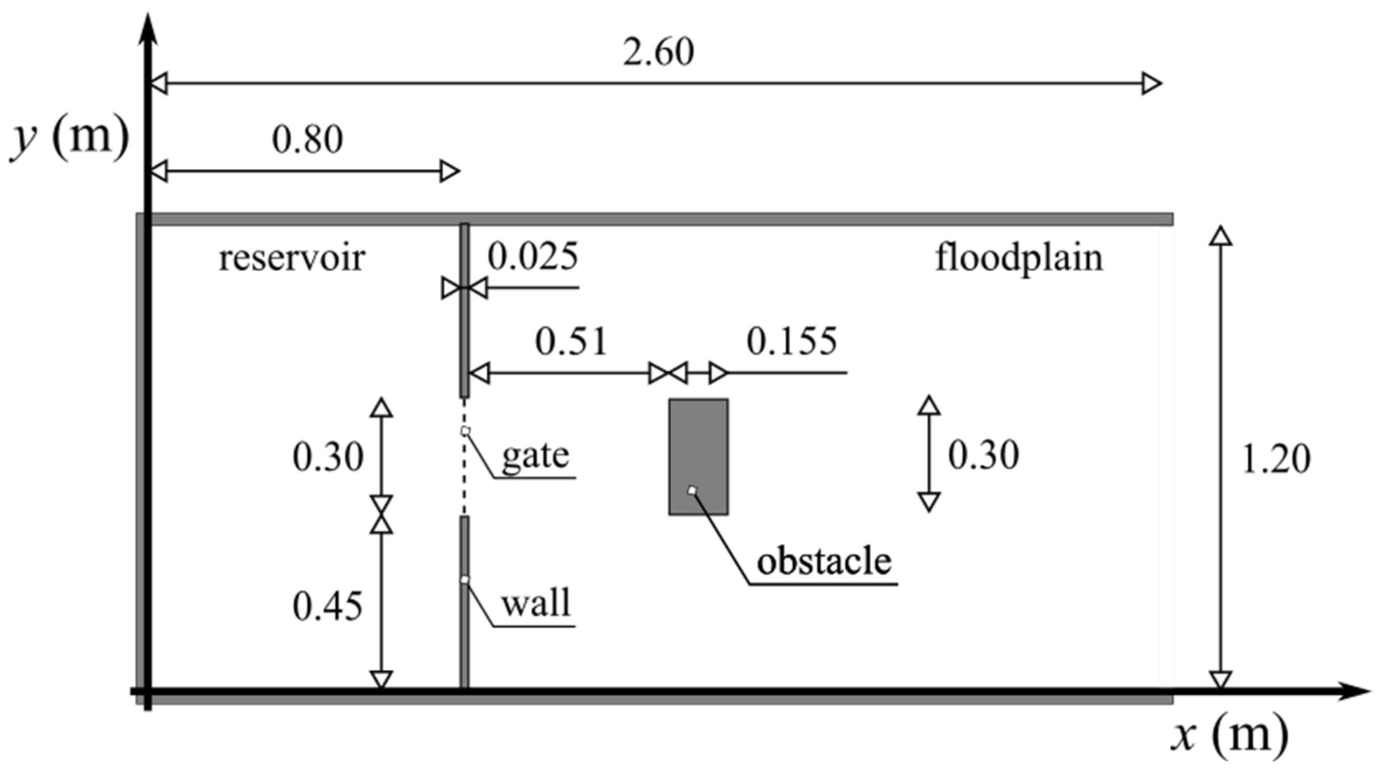
2.4. The Test Case

Figure 1 reproduces the geometry of the experimental test case by Aureli et al. [19] used for clear-water dam-break experiments on a fixed bottom. The initial water level in the reservoir is ${\mathrm{h}}_0 = 0.10 \mathrm{m}$ and flow is triggered by the sudden removal of the gate, which produces the propagation of a dam-break wave over the downstream floodable area. The performance of both models for the clear-water case has been preliminarily verified against the experimental data by Aureli et al. [19].

In the present numerical simulations, the floodplain is assumed constituted by loose sediment, and two different kinds of solid particles are considered: a uniformly graded sand (density ${\mathsf{\rho }}_{\mathrm{s}} = 2650 \mathrm{kg}/{\mathrm{m}}^3$) and very light sediment (PVC) (density ${\mathsf{\rho }}_{\mathrm{s}} = 1540 \mathrm{kg}/{\mathrm{m}}^3$). For each material, two scenarios have been considered by changing the sediment diameter from d = 5 × 10⁻⁴ m to d = 5 × 10⁻³ m.

The simulations with sand on the bottom aim to compare the performance of the two models at the laboratory scale. Although this procedure is widely used in the literature to benchmark numerical models, owing to the incomplete Froude similarity, the simulated results cannot be straightforwardly extended to realistic cases in which the bed particles are still sand. This limitation may be overcome considering sediment lighter than sand, such as PVC, which allows satisfying the equality between the model and the prototype of both the hydrodynamic and the particle densimetric Froude numbers:

$$\mathrm{F} = \frac{{\mathrm{U}}_{\mathrm{ref}}}{\sqrt{{\mathrm{gh}}_{\mathrm{ref}}}}, {\mathrm{F}}_{\mathrm{d}} = \frac{{\mathrm{U}}_{\mathrm{ref}}}{\sqrt{\mathrm{grd}}}$$

(28)

in which the reference length scale is assumed as ${\mathrm{h}}_{\mathrm{ref}} = {\mathrm{h}}_0$ and the velocity scale as ${ \mathrm{U}}_{\mathrm{ref}} = \sqrt{{\mathrm{gh}}_{\mathrm{ref}}}$. For example, accounting for the Froude similarity, the tests with d = 5 × 10⁻³ m and d = 5 × 10⁻⁴ m in PVC can be upscaled to a realistic dam-break wave with an initial height in the reservoir ${\mathrm{h}}_0 = 3 \mathrm{m}$ and involving gravel with d = 5 × 10⁻² m and sand with d = 5 × 10⁻³ m, respectively. The good performance of the two-phase model with the PVC particles adopted in this study has been already tested [51] in reproducing the experimental dam-break phenomenon investigated by [52]. Similarly, for the sand particles, the two-phase model was benchmarked under different test cases [24,46].

In the numerical simulations the following values of the parameters are assumed: ${\mathsf{\mu }}_{\mathrm{d}} = 25°$, ${\mathsf{\mu }}_0 = 38°$, ${\mathrm{K}}_{\mathrm{MPM}} = 8$ and ${\mathrm{c}}_1 = 0.25$, ${\mathrm{C}}_{\mathrm{Ch}}= 12$. A computational mesh with $∆\mathrm{x} = ∆\mathrm{y} = 5·{10}^{-3} \mathrm{m}$ is used along with $∆\mathrm{t} = 1/2048 \mathrm{s}$. The accuracy of the numerical solutions has been tested halving the mesh spacing and the time step: the sensitivity of the predicted maximum impact force resulted to be less than 0.1 N for all the investigated conditions, with the only exception of SVEM simulation for the sand with d = 5 × 10⁻⁴ m, where a difference of 0.3 N was found.

It is worthy of note that the different complexity of the two models implies a higher computational cost for the TPM compared to the SVEM. In the present simulations, carried out on a single core of an Intel(R) i7-7700 CPU at 3.60 GHz equipped with 16 GB RAM, the CPU time per iteration resulted in 0.062 s for the SVEM and 0.094 s for the TPM, meaning an increase in the computational effort of about 52%.

3. Results and Discussion

3.1. Force Evaluation

The comparison between the coupled equilibrium and the two-phase models mainly aims to investigate their performance in evaluating the impact force on an obstacle. For a more complete understanding, the simulated free-surface (${\mathrm{z}}_{\mathrm{w}}$) and bottom (${\mathrm{z}}_{\mathrm{B}}$) evolution are also compared.

Based on the simulated flow fields, in processing the results of the TPM, the impact force $\mathbf{F}$ is evaluated by numerically computing the following integral.

$${ \mathbf{F} = \mathsf{\rho }}_{\mathrm{l}}\underset{\mathsf{\sigma }}{\overset{}{{\displaystyle \int }}}\left({\mathsf{\delta }}_{\mathrm{l}}{\mathbf{U}}_{\mathrm{l}}{\mathrm{U}}_{\mathrm{l},\mathrm{n}}+\frac{{\mathrm{gh}}^2}{2}\hat{\mathbf{n}}\right){\mathrm{d}\mathsf{\sigma } + \mathsf{\rho }}_{\mathrm{s}}\underset{\mathsf{\sigma }}{\overset{}{{\displaystyle \int }}}\left({\mathsf{\delta }}_{\mathrm{s}}{\mathbf{U}}_{\mathrm{s}}{\mathrm{U}}_{\mathrm{s},\mathrm{n}}+\frac{\mathrm{r}}{\mathrm{r}+1}\frac{{\mathrm{g}\mathsf{\delta }}_{\mathrm{s}}{\mathrm{K}}_{\mathrm{s}}\mathrm{d}}{2}\hat{\mathbf{n}}\right)\mathrm{d}\mathsf{\sigma } + \underset{\mathsf{\sigma }}{\overset{}{{\displaystyle \int }}}\left[{\mathsf{\rho }}_{\mathrm{l}}\mathrm{g}\left(\mathrm{h}+\frac{∆}{2}\right)∆+\left({\mathsf{\rho }}_{\mathrm{B}}-{\mathsf{\rho }}_{\mathrm{l}}\right)\frac{\mathrm{g}{∆}^2}{2}\right]\hat{\mathbf{n}} \mathrm{d}\mathsf{\sigma }$$

(29)

where $\mathsf{\sigma }$ denotes the boundary of the obstacle and $\hat{\mathbf{n}}$ is the corresponding normal unit vector. The last term accounts for the contribution of the height of the deposited sediment, $∆$, in contact with the upstream face of the obstacle, whose bulk density is ${\mathsf{\rho }}_{\mathrm{B}}{ = \mathrm{p}\mathsf{\rho }}_{\mathrm{l}}+\left(1-\mathrm{p}\right){\mathsf{\rho }}_{\mathrm{s}}$. The values of the flow variables in the cells adjacent to the obstacle are used in Equation (29). As far as the Saint–Venant–Exner model is concerned, the impact force has been evaluated neglecting the contribution of the solid phase, i.e., through Equation (29), setting ${\mathsf{\delta }}_{\mathrm{s}} ={ \mathbf{U}}_{\mathrm{s}} = 0,$ ${\mathsf{\delta }}_{\mathrm{l}} = \mathrm{h}$ and ${\mathbf{U}}_{\mathrm{l}}{ = \mathbf{q}}_{\mathrm{l}}/\mathrm{h}$.

3.2. Simulations with Sand

For the tests with sand, Figure 2 compares the impact forces evaluated through the two models for both the considered diameters. In all the considered simulations, the wave impacts the obstacle at $\mathrm{t} ~ 0.5 \mathrm{s}$, and the maximum force occurs for $\mathrm{t} ~ 1.5 \mathrm{s}$. For both diameter values, the results indicate higher force values predicted by the SVEM, with more evident differences for the fine particles. In fact, the two-phase model predicts a maximum value of the impact force, which is about 4–13% smaller than the maximum value predicted by the SVEM for the coarse and fine particles, respectively.

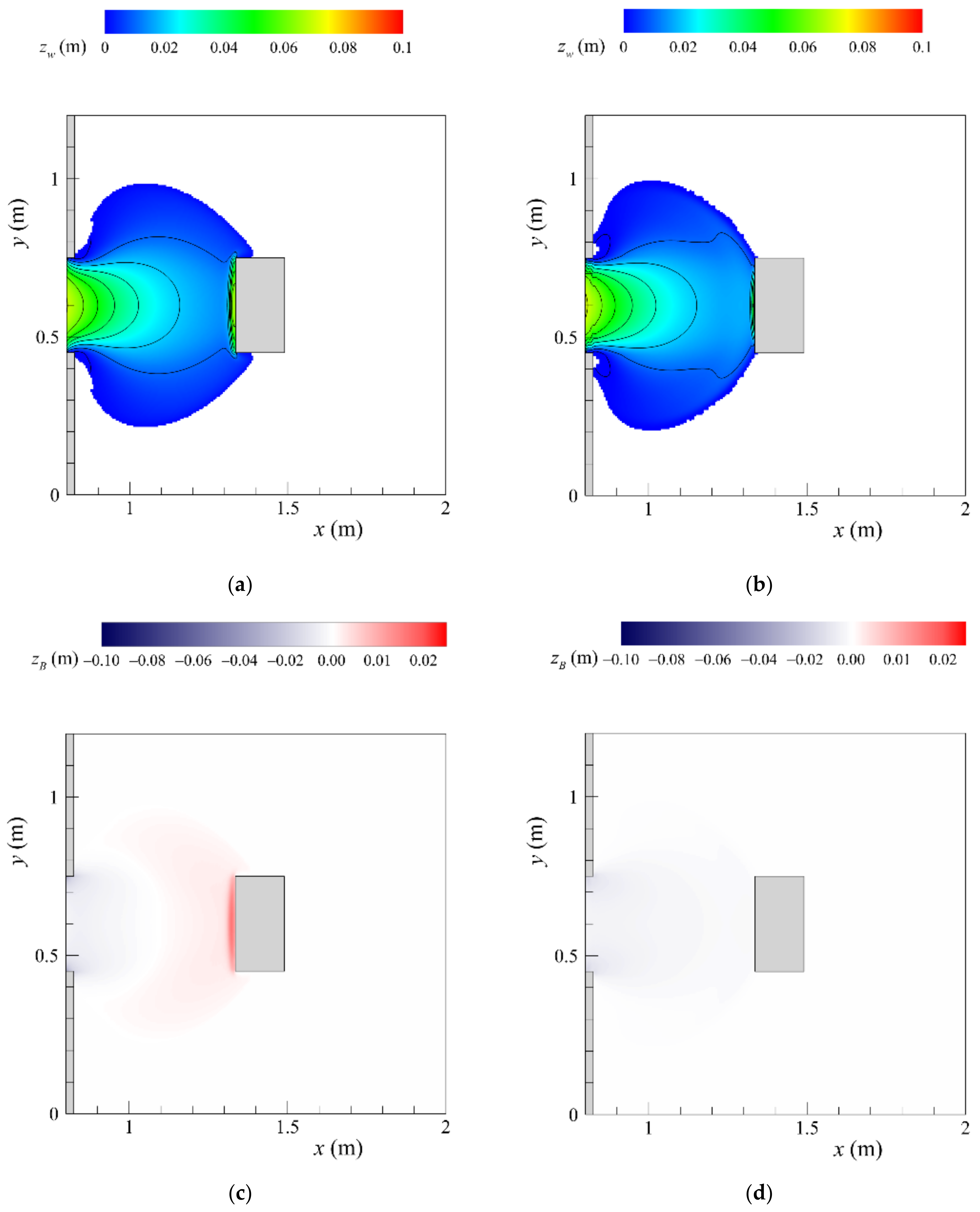
The two models similarly reproduce the free-surface and bottom evolution for the coarse sand, and some differences are observed for the fine particles. For example, Figure 3 and Figure 4 illustrate the free-surface and bottom elevation predicted by the SVEM and the TPM, for the coarse and fine sediments, respectively, at $\mathrm{t} = 1.5 \mathrm{s}$, when the largest differences between the two models are observed. For the same instant, Figure 5 reports the longitudinal profile of the free-surface and bottom elevation at y = B/2, where symmetry imposes ${\mathrm{U}}_{\mathrm{l},\mathrm{y}}{ = \mathrm{U}}_{\mathrm{s},\mathrm{y}}= 0$.

After the impact, the flow depth increases, and the shear stress drops below the critical value for sediment transport producing a deposit close to the obstacle. For the coarse sand (Figure 3c,d and Figure 5a), the results of the two models are very close to each other, and both predict a comparable deposition upstream of the obstacle and close to the flume walls. For the fine particles (Figure 4c,d and Figure 5b), the highest water depth is predicted by the equilibrium model, and some differences are observed in terms of bed evolution. Figure 5b indicates that the SVEM predicts a higher deposit upstream of the obstacle than the TPM.

Moreover, it is observed that the flow remains supercritical while running up onto the bump, and then the subcritical flow depth increases with the bump height, as predicted under the hypothesis of negligible momentum loss of the approaching flow. The increase of impact force observed in the results of SVEM (Figure 2) is therefore explainable as a direct consequence of the presence of a higher deposit in contact with the obstacle, combined with a higher flow depth.

Taken collectively, the above results show that in the case of sand the simplest SVEM performs similarly to the more complex, and computationally expensive, TPM, in particular in reproducing the impact force. This is consistent with what was observed by other authors in analyzing different laboratory experiments involving dam-break waves over erodible sand bottoms [36,53,54].

3.3. Simulations with PVC

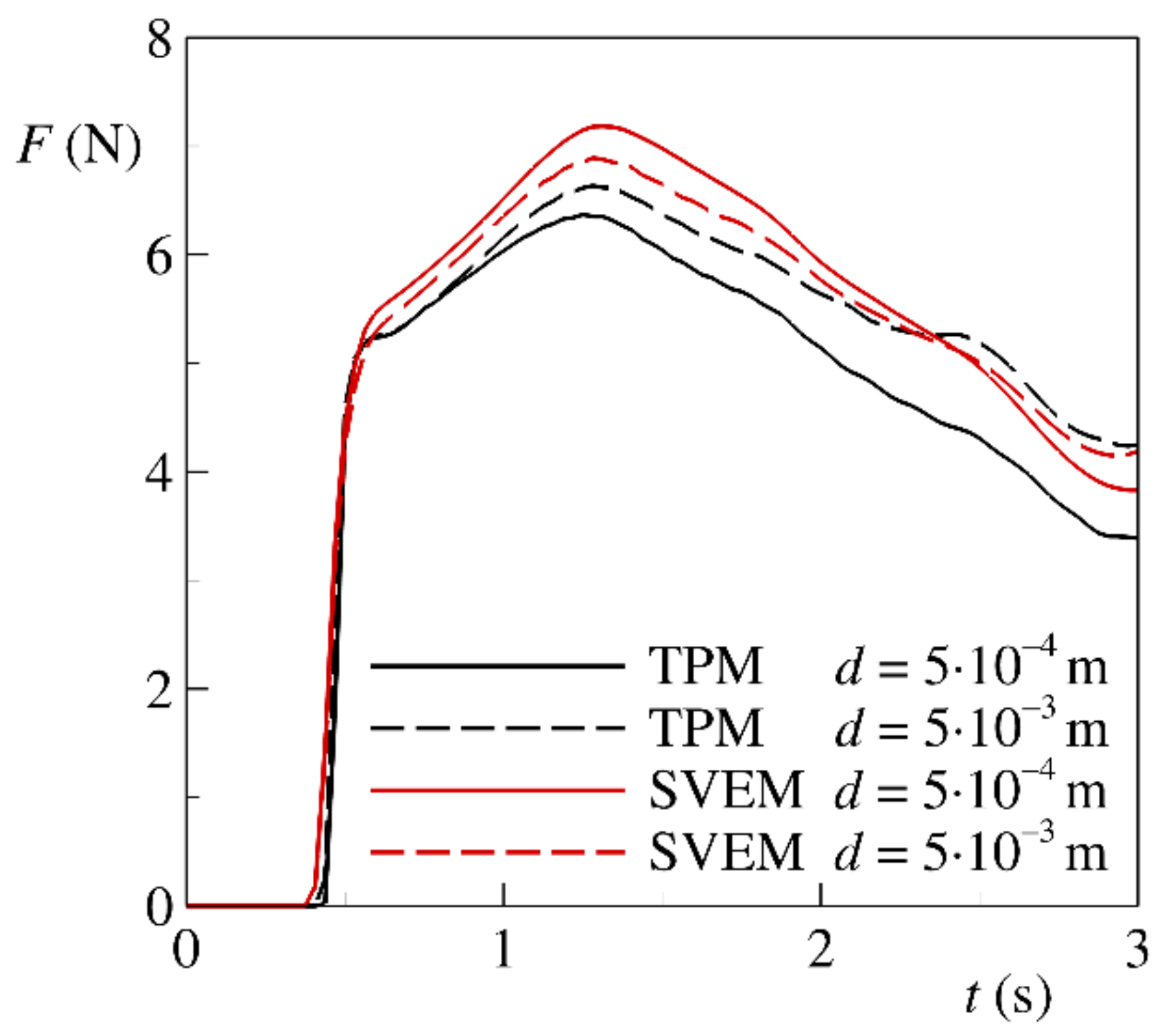
For the PVC sediment, Figure 6 reports the temporal evolution of the impact force against the obstacle predicted by the two models for the two considered sediment diameters. In both models, the effect of the particle diameter in the force evolution is very marginal, without significant differences in the estimated maximum value. Differently from the sand, larger differences are observed between the two models, with SVEM that predicts a maximum force in excess of about 26%, with respect to the TPM.

The differences in the impact force motivate a deep comparison of the results of hydrodynamic and morphodynamic simulations, performed through the analysis of the temporal evolution of the free-surface and bottom elevation. Considering the case with the fine particles, where the differences are more pronounced, Figure 7, Figure 8, Figure 9 and Figure 11 illustrate the free-surface and bottom elevation contour maps for t = 0.5 s, t = 1.0 s, t = 1.5 s and t = 3.0 s, respectively. The detailed analysis of the plots at different instants indicates that the development of the wave originating by the dam-break can be divided into three phases: approaching, reflecting and reservoir emptying phases. The last phase ($\mathrm{t} > 3.0 \mathrm{s}$) is out of the scope of the present investigation and will not be discussed.

In the approaching phase ($\mathrm{t} \le 0.5 \mathrm{s}$), the dam-break wave spreads over the erodible floodplain up to the impact with the obstacle, which occurs at $\mathrm{t} ~ 0.5 \mathrm{s}$. At the impact (Figure 7), in terms of free-surface evolution, small differences are observed between the two models. However, during this phase, the fluid decelerates in the downstream tail of the wave due to the lateral expansion. This behavior produces different consequences according to the sediment transport description of the morphodynamic model. In the equilibrium model, the Exner equation dictates that the flow entrains sediment in the accelerating region of the wave, whereas it deposits while decelerating. This produces an excavation close to the gate and a deposit upstream of the obstacle, as illustrated in Figure 7c. For the dynamic model, the bed evolution is modeled based on the erosion and deposition terms in Equation (17) and the bed-load dynamics. In fact, Figure 7d shows that the erosion prevails, and no deposition is observed until t = 0.5 s.

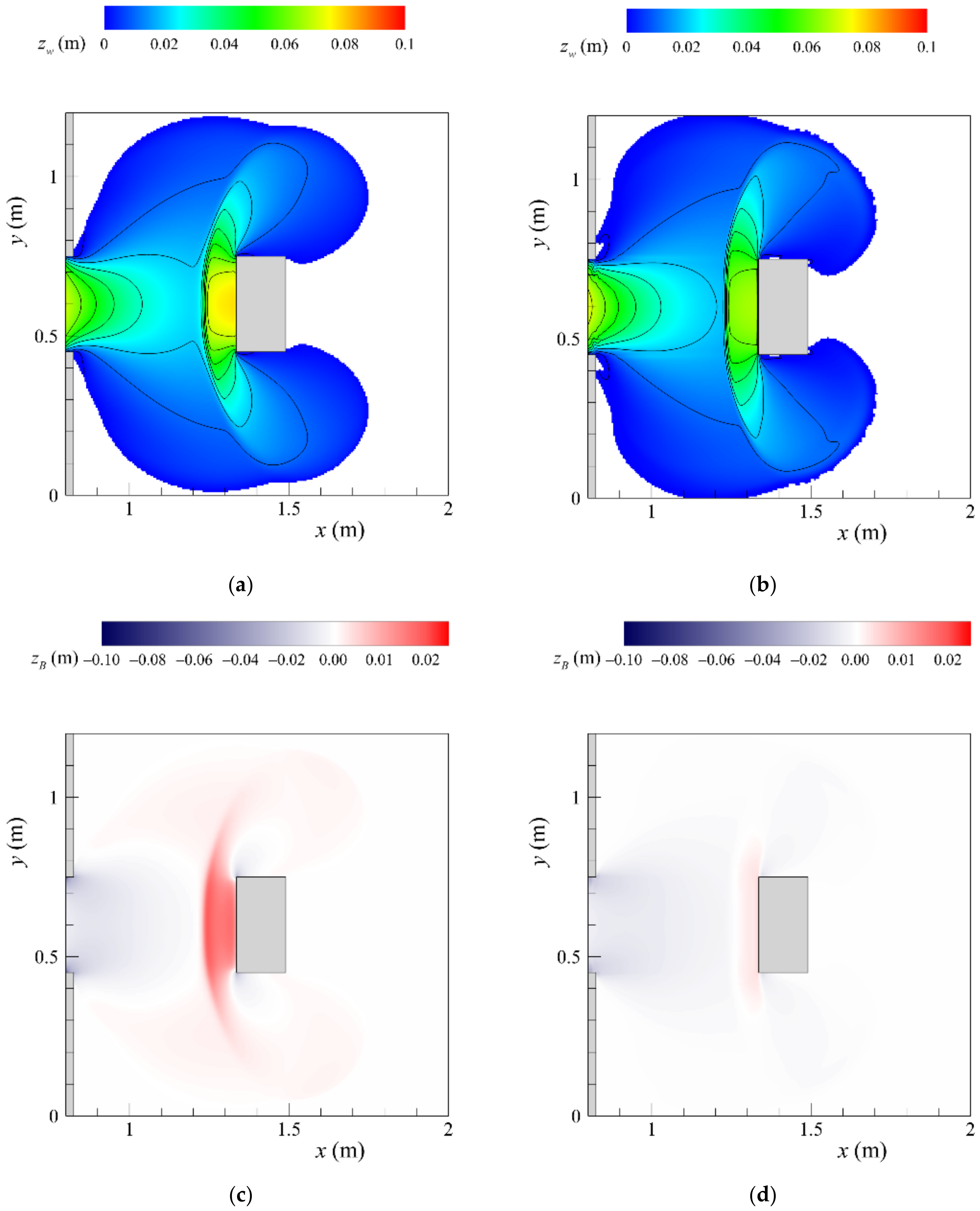
In the second phase ($0.5 < \mathrm{t} \le 3.0 \mathrm{s}$), a reflected wave forms against the upstream face of the obstacle (Figure 8, Figure 9 and Figure 11). The wave develops as a receding bore between t = 0.5 s and t = 1.0 s and turns into a kind of stationary jump for $\mathrm{t} > 1.0 \mathrm{s}$. At t = 1.0 s (Figure 8a,b), the wave surrounds the obstacle and further expands laterally, reaching the lateral walls. Then, at t = 1.5 s (Figure 9), the wave impacts the sidewalls with a lateral deflection, and two wave fronts are generated. Successively, the wave reaches the flume outlet and leaves a large dry region behind the obstacle (Figure 11). For $1.0 < \mathrm{t} \le 2.0 \mathrm{s}$, while the wave front position is similarly reproduced by the two models, some differences are observed in terms of free-surface elevation upstream of the obstacle, with higher levels predicted by the equilibrium model. The differences are more evident at t = 1.5 s (Figure 9a,b). Moreover, while both models predict a deposition in front of the obstacle and close to the sidewalls, this effect is more pronounced for the equilibrium model (Figure 9c,d).

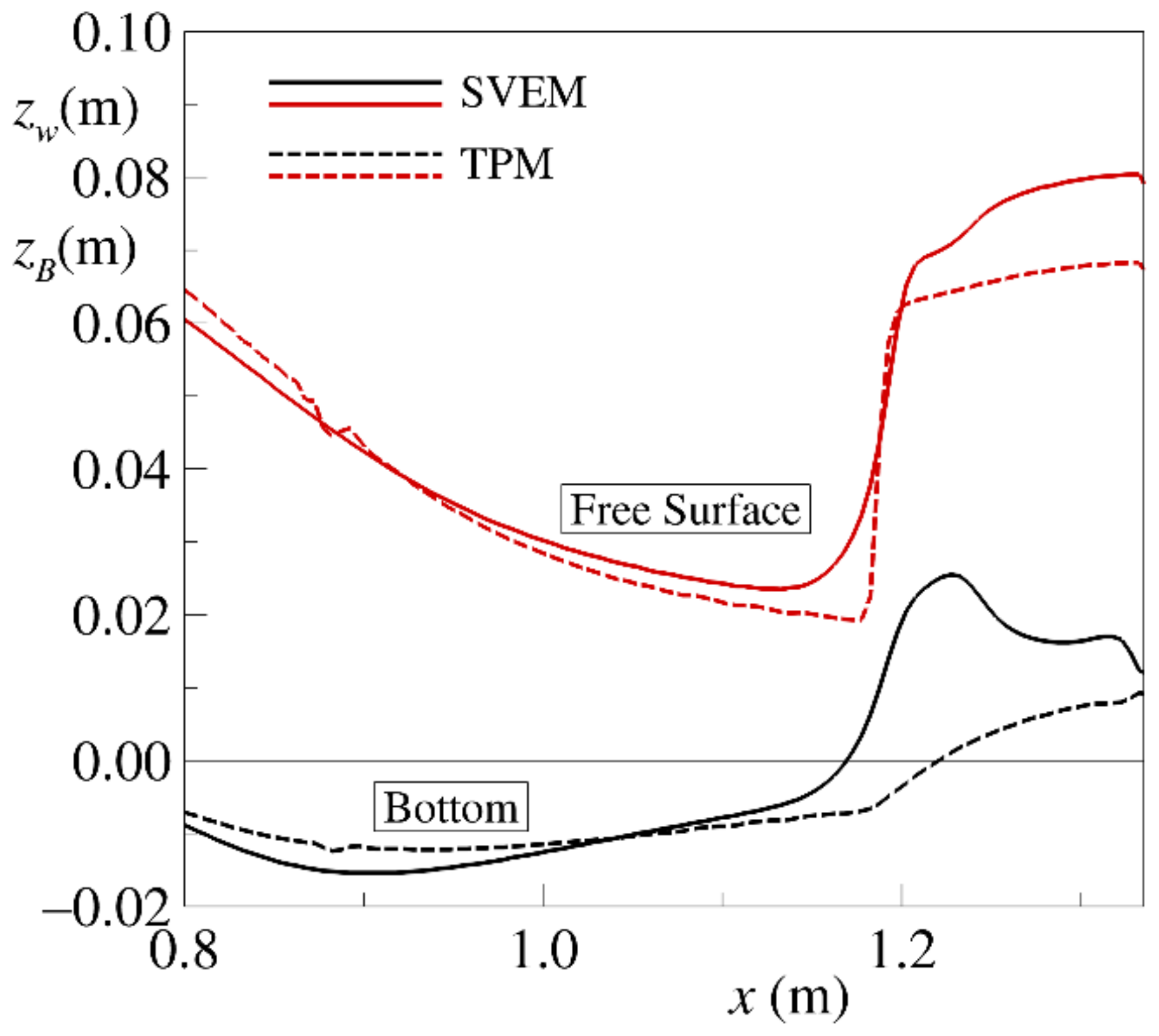
To gain some insights on this behavior, Figure 10 reports the longitudinal profile at y = B/2 of the free-surface and bed elevation at t = 1.5 s. The two models furnish similar qualitative predictions in terms of both the free-surface and bottom elevation but with a quantitative difference. As shown in Figure 10, the deposit simulated by the SVEM is about five times that of the two-phase model, with a consequent higher flow depth of about 17%.

For t = 3.0 s, the two wave fronts merge downstream of the obstacle, leaving a small dry region (Figure 11). Some differences are noted in the hydrodynamics, with the two-phase model predicting a wider dry zone and no deposition downstream of the obstacle. A higher deposit is simulated by the equilibrium model downstream of the obstacle and at the channel walls.

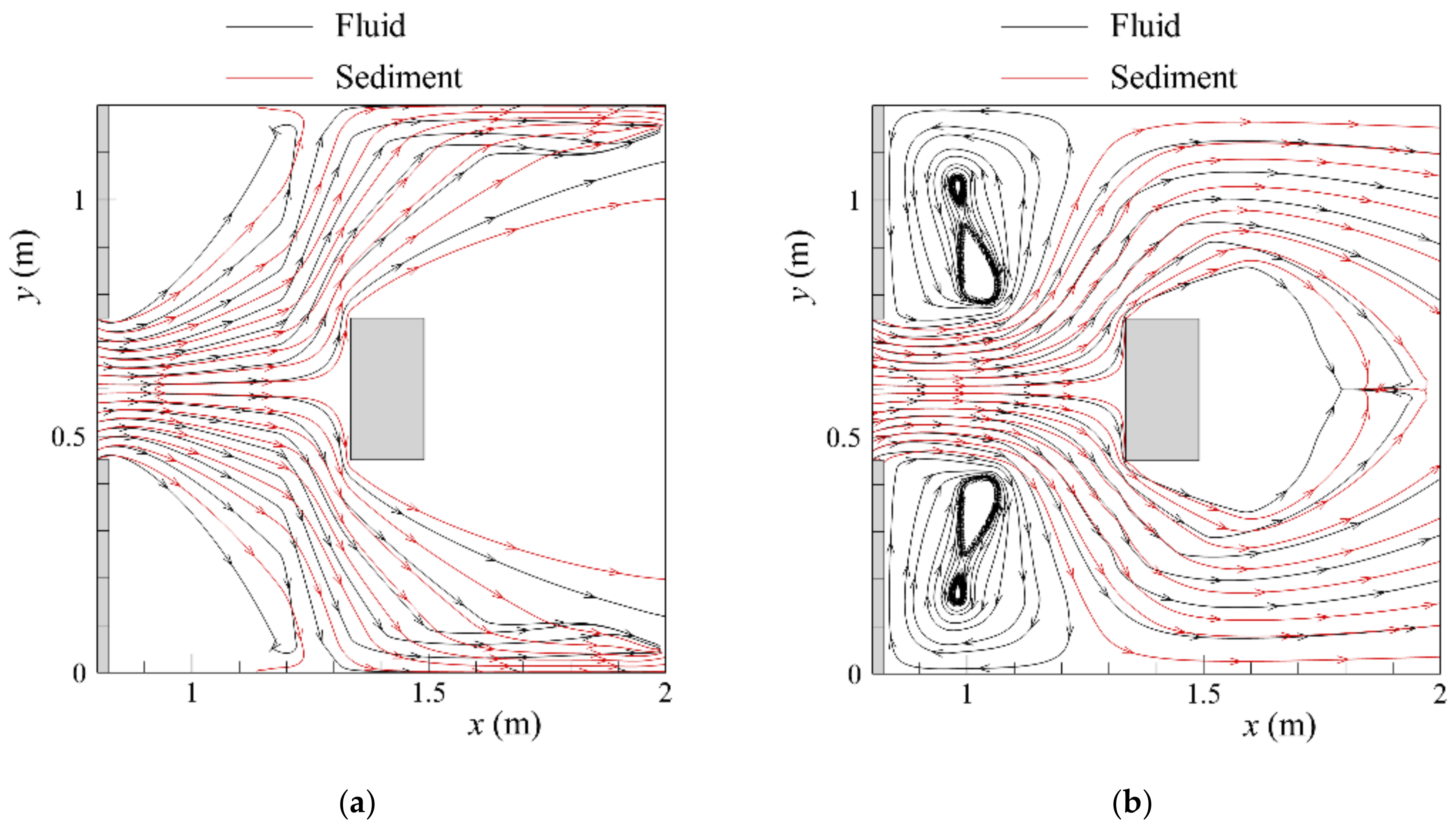
To complete the discussion about the two-phase modeling performance, Figure 12 reports the fluid and solid streamlines at t = 1.5 s and t = 3.0 s. At both times, a misalignment of the streamlines of the two phases is detected both upstream and downstream of the obstacle. It is more evident downstream when the flow splits into two parts, while at t = 3.0 s, only in the water flow field is recirculation observed in the region close to the dam. These results indicate some resistance, for the considered application, of the PVC sediment to adapt to the change in the flow direction imposed by the carrying fluid, a feature that cannot be represented by the SVE model.

As a final remark, it is noted the set of TPM closures guarantees that it collapses on the SVEM as transport reaches equilibrium. The similar behavior of the two models for the tests with sand therefore is consistent with a minor role of sediment inertia. Conversely, with the PVC, the sensible difference in evaluating the impact force and the misalignment of the streamlines reveal that the sediment dynamics are not negligible.

Furthermore, the shown dependence of the performance of the SVEM on the sediment density may be theoretically justified based on the governing ratio of the geomorphic timescale (${\mathrm{t}}_{\mathrm{g}}$) to the hydrodynamic (${\mathrm{t}}_{\mathrm{h}}$) timescale. Indeed, considering the ratio of the geomorphic to the hydrodynamic timescale to be of the order of $1/\mathrm{r}$ [55], it follows that ${\mathrm{t}}_{\mathrm{g}}/{\mathrm{t}}_{\mathrm{h}}$ increases from 0.6 (sand) up to 2 (PVC) in the two tests. The smaller geomorphic time scale in the sand tests suggests a more rapid adaptation of the sediment to the hydrodynamics, complying better with the equilibrium assumption.

4. Conclusions

The definition of effective tools for the prediction of the impact force on structures due to floods is very important for the implementation of appropriate risk mitigation strategies and the design of protection countermeasures. The present study compares the outcomes of two morphodynamic models, analyzing the interaction of a dam-break wave against a rigid obstacle in the presence of an erodible bed. The first morphodynamic model is the widespread, two-dimensional Saint–Venant–Exner model, which assumes local equilibrium conditions of the solid transport. The second model belongs to the class of nonequilibrium models and is based on a two-phase schematization. Although the latter model allows a more accurate description of the morphodynamic processes than the former, it is characterized by a much larger computational cost. The comparison was carried out varying both the diameter and density of the erodible bed particles. The tests performed with heavy particles, i.e., sand, directly referred to a common laboratory condition, and the tests with reduced particle density, i.e., PVC, can be considered representative of a field-scale based on the Froude similarity. As far as the sand particles tests are concerned, the present results indicate that, independently of the particle diameters, the predictions of the two models only slightly differ in terms of impact forces. Moreover, only marginal differences are visible in terms of hydrodynamics and morphodynamics. This is consistent with previous studies, which have shown that the performance of the Saint–Venant–Exner model is comparable with those of nonequilibrium models in the reproduction of laboratory experiments with sand. Different conclusions have been drawn considering the tests with light particles. Indeed, the differences between the impact forces increase up to about 30%, with the largest value pertaining to the Saint–Venant–Exner model. A deep analysis of the flow field and morphodynamics allowed relating these changes to the different deposition mechanism of the solid particles in front of the obstacle.

Future research will be devoted to further extend and generalize the above results, addressing the application of uncoupled solution strategies for the two-dimensional Saint–Venant–Exner model and the investigation of coupled and uncoupled approaches, with reference also to other test cases characterized by different geometries and/or arrangements of the obstacles. Furthermore, future research will be devoted to the study of the impact of debris and mudflows on obstacles accounting for both fixed and mobile bed conditions.

References

- Fuchs, S. Susceptibility versus resilience to mountain hazards in Austria—Paradigms of vulnerability revisited. Nat. Hazards Earth Syst. Sci. 2009, 9, 337–352. [Google Scholar] [CrossRef]
- Keiler, M.; Fuchs, S. Vulnerability and exposure to geomorphic hazards: Some insights from the European alps. In Geomorphology and Society; Meadows, M.E., Lin, J.-C., Eds.; Springer: Tokyo, Japan, 2016; pp. 165–180. [Google Scholar]
- Stoffel, M.; Wyżga, B.; Marston, R.A. Floods in mountain environments: A synthesis. Geomorphology 2016, 272, 1–9. [Google Scholar] [CrossRef]
- Slaymaker, O.; Embleton-Hamann, C. Advances in global mountain geomorphology. Geomorphology 2018, 308, 230–264. [Google Scholar] [CrossRef]
- Sturm, M.; Gems, B.; Keller, F.; Mazzorana, B.; Fuchs, S.; Papathoma-Köhle, M.; Aufleger, M. Understanding impact dynamics on buildings caused by fluviatile sediment transport. Geomorphology 2018, 321, 45–59. [Google Scholar] [CrossRef]
- Hoerling, M.P. Tropical origins for recent north atlantic climate change. Science 2001, 292, 90–92. [Google Scholar] [CrossRef] [Green Version]
- Keiler, M.; Knight, J.; Harrison, S. Climate change and geomorphological hazards in the eastern European Alps. Philos. Trans. R. Soc. A 2010, 368, 2461–2479. [Google Scholar] [CrossRef] [Green Version]
- Fuchs, S.; Keiler, M.; Zischg, A. A spatiotemporal multi-hazard exposure assessment based on property data. Nat. Hazards Earth Syst. Sci. 2015, 15, 2127–2142. [Google Scholar] [CrossRef] [Green Version]
- Thieken, A.H.; Müller, M.; Kreibich, H.; Merz, B. Flood damage and influencing factors: New insights from the August 2002 flood in Germany: Flood damage and influencing factors. Water Resour. Res. 2005, 41, W12430. [Google Scholar] [CrossRef]
- Quan Luna, B.; Blahut, J.; van Westen, C.J.; Sterlacchini, S.; van Asch, T.W.J.; Akbas, S.O. The application of numerical debris flow modelling for the generation of physical vulnerability curves. Nat. Hazards Earth Syst. Sci. 2011, 11, 2047–2060. [Google Scholar] [CrossRef] [Green Version]
- Totschnig, R.; Sedlacek, W.; Fuchs, S. A quantitative vulnerability function for fluvial sediment transport. Nat. Hazards 2011, 58, 681–703. [Google Scholar] [CrossRef] [Green Version]
- Totschnig, R.; Fuchs, S. Mountain torrents: Quantifying vulnerability and assessing uncertainties. Eng. Geol. 2013, 155, 31–44. [Google Scholar] [CrossRef] [PubMed] [Green Version]
- Papathoma-Köhle, M.; Keiler, M.; Totschnig, R.; Glade, T. Improvement of vulnerability curves using data from extreme events: Debris flow event in South Tyrol. Nat. Hazards 2012, 64, 2083–2105. [Google Scholar] [CrossRef]
- Papathoma-Köhle, M.; Zischg, A.; Fuchs, S.; Glade, T.; Keiler, M. Loss estimation for landslides in mountain areas—An integrated toolbox for vulnerability assessment and damage documentation. Environ. Model. Softw. 2015, 63, 156–169. [Google Scholar] [CrossRef]
- Shige-eda, M.; Akiyama, J. Numerical and experimental study on two-dimensional flood flows with and without structures. J. Hydraul. Eng. 2003, 129, 817–821. [Google Scholar] [CrossRef]
- Bukreev, V.I. Force action of discontinuous waves on a vertical wall. J. Appl. Mech. Tech. Phys. 2009, 50, 278–283. [Google Scholar] [CrossRef]
- Soares-Frazão, S.; Zech, Y. Dam-break flow through an idealised city. J. Hydraul. Res. 2008, 46, 648–658. [Google Scholar] [CrossRef] [Green Version]
- El Kadi Abderrezzak, K.; Paquier, A.; Mignot, E. Modelling flash flood propagation in urban areas using a two-dimensional numerical model. Nat. Hazards 2009, 50, 433–460. [Google Scholar] [CrossRef]
- Aureli, F.; Dazzi, S.; Maranzoni, A.; Mignosa, P.; Vacondio, R. Experimental and numerical evaluation of the force due to the impact of a dam-break wave on a structure. Adv. Water Resour. 2015, 76, 29–42. [Google Scholar] [CrossRef]
- Gao, L.; Zhang, L.M.; Chen, H.X. Two-dimensional simulation of debris flow impact pressures on buildings. Eng. Geol. 2017, 226, 236–244. [Google Scholar] [CrossRef]
- Kattel, P.; Kafle, J.; Fischer, J.-T.; Mergili, M.; Tuladhar, B.M.; Pudasaini, S.P. Interaction of two-phase debris flow with obstacles. Eng. Geol. 2018, 242, 197–217. [Google Scholar] [CrossRef]
- Greco, M.; Di Cristo, C.; Iervolino, M.; Vacca, A. Numerical simulation of mud-flows impacting structures. J. Moutain Sci. 2019, 16, 364–382. [Google Scholar] [CrossRef]
- Di Cristo, C.; Greco, M.; Lervolino, M.; Vacca, A. Interaction of a dam-break wave with an obstacle over an erodible floodplain. J. Hydroinform. 2020, 22, 5–19. [Google Scholar] [CrossRef]
- Di Cristo, C.; Greco, M.; Iervolino, M.; Leopardi, A.; Vacca, A. Two-dimensional two-phase depth-integrated model for transients over mobile bed. J. Hydraul. Eng. 2016, 142, 4015043. [Google Scholar] [CrossRef] [Green Version]
- Dewals, B.; Rulot, F.; Erpicum, S.; Archambeau, P.; Pirotto, M. Advanced topics in sediment transport modelling: Non-alluvial beds and hyperconcentrated flows. In Sediment Transport; Ginsberg, S.S., Ed.; InTech: London, UK, 2011. [Google Scholar]
- Greco, M.; Iervolino, M.; Leopardi, A.; Vacca, A. A two-phase model for fast geomorphic shallow flows. Int. J. Sediment Res. 2012, 27, 409–425. [Google Scholar] [CrossRef]
- Rosatti, G.; Begnudelli, L. A closure-independent Generalized Roe solver for free-surface, two-phase flows over mobile bed. J. Comput. Phys. 2013, 255, 362–383. [Google Scholar] [CrossRef]
- Wu, W.; Wang, S.S. One-dimensional modeling of dam-break flow over movable beds. J. Hydraul. Eng. 2007, 133, 48–58. [Google Scholar] [CrossRef]
- Capart, H. Young two-layer shallow water computations of torrential geomorphic flows. In Proceedings of the River Flow 2002, Louvain La Neuve, Belgium, 4–6 September 2002; pp. 1003–1012. [Google Scholar]
- Savary, C.; Zech, Y. Boundary conditions in a two-layer geomorphological model. Application to a. J. Hydraul. Res. 2007, 45, 316–332. [Google Scholar] [CrossRef]
- Li, J.; Cao, Z.; Pender, G.; Qingquan, L. A double layer-averaged model for dam-break flows over mobile bed. J. Hydraul. Res. 2013, 51, 518–534. [Google Scholar] [CrossRef] [Green Version]
- Swartenbroekx, C.; Zech, Y.; Soares-Frazão, S. Two-dimensional two-layer shallow water model for dam break flows with significant bed load transport. Int. J. Numer. Methods Fluids 2013, 73, 477–508. [Google Scholar] [CrossRef]
- Graf, W.H.; Altinakar, M.S. Fluvial Hydraulics: Flow and Transport Processes in Channels of Simple Geometry; Wiley: Chichester, UK; New York, NY, USA, 1998. [Google Scholar]
- Aricò, C.; Tucciarelli, T. Diffusive modeling of aggradation and degradation in artificial channels. J. Hydraul. Eng. 2008, 134, 1079–1088. [Google Scholar] [CrossRef]
- Juez, C.; Murillo, J.; García-Navarro, P. A 2D weakly-coupled and efficient numerical model for transient shallow flow and movable bed. Adv. Water Resour. 2014, 71, 93–109. [Google Scholar] [CrossRef]
- Soares-Frazão, S.; Zech, Y. HLLC scheme with novel wave-speed estimators appropriate for two-dimensional shallow-water flow on erodible bed. Int. J. Numer. Methods Fluids 2011, 66, 1019–1036. [Google Scholar] [CrossRef]
- Meurice, R.; Soares-Frazão, S. A 2D HLL-based weakly coupled model for transient flows on mobile beds. J. Hydroinform. 2020, 22, 1351–1369. [Google Scholar] [CrossRef]
- Soares-Frazão, S.; Canelas, R.; Cao, Z.; Cea, L.; Chaudhry, H.M.; Moran, A.D.; Kadi, K.E.; Ferreira, R.; Cadórniga, I.F.; Gonzalez-Ramirez, N.; et al. Dam-break flows over mobile beds: Experiments and benchmark tests for numerical models. J. Hydraul. Res. 2012, 50, 364–375. [Google Scholar] [CrossRef]
- Sturm, M.; Gems, B.; Aufleger, M.; Mazzorana, B.; Papathoma-Köhle, M.; Fuchs, S. Scale model measurements of impact forces on obstacles induced by bed-load transport processes. In Proceedings of the 37th IAHR World Congress, Kuala Lumpur, Malaysia, 13–18 August 2017; pp. 1459–1468. [Google Scholar]
- Meyer-Peter, E.; Müller, R.M. Formulas for bed-load transport. In Proceedings of the IAHSR 2nd Meeting, Stockholm, Sweden, 7–9 June 1948; Appendix 2. pp. 39–64. [Google Scholar]
- Cordier, S.; Le, M.H.; Morales de Luna, T. Bedload transport in shallow water models: Why splitting (may) fail, how hyperbolicity (can) help. Adv. Water Resour. 2011, 34, 980–989. [Google Scholar] [CrossRef] [Green Version]
- Carraro, F.; Valiani, A.; Caleffi, V. Efficient analytical implementation of the DOT Riemann solver for the de Saint Venant–Exner morphodynamic model. Adv. Water Resour. 2018, 113, 189–201. [Google Scholar] [CrossRef] [Green Version]
- Pontillo, M.; Schmocker, L.; Greco, M.; Hager, W.H. 1D numerical evaluation of dike erosion due to overtopping. J. Hydraul. Res. 2010, 48, 573–582. [Google Scholar] [CrossRef]
- Richardson, J.F.; Zaki, W.N. Sedimentation and fluidisation: Part I. Chem. Eng. Res. Des. 1997, 75, S82–S100. [Google Scholar] [CrossRef]
- Van Rijn, L.C. Sediment pick-up functions. J. Hydraul. Eng. 1984, 110, 1494–1502. [Google Scholar] [CrossRef]
- Di Cristo, C.; Evangelista, S.; Greco, M.; Iervolino, M.; Leopardi, A.; Vacca, A. Dam-break waves over an erodible embankment: Experiments and simulations. J. Hydraul. Res. 2018, 56, 196–210. [Google Scholar] [CrossRef]
- Barth, T.; Jespersen, D. The design and application of upwind schemes on unstructured meshes. In Proceedings of the 27th Aerospace Sciences Meeting, Reno, NV, USA, 9–12 January 1989. [Google Scholar]
- Nikolos, I.K.; Delis, A.I. An unstructured node-centered finite volume scheme for shallow water flows with wet/dry fronts over complex topography. Comput. Methods Appl. Mech. Eng. 2009, 198, 3723–3750. [Google Scholar] [CrossRef]
- Harten, A.; Lax, P.D.; Leer, B. Van on upstream differencing and Godunov-type schemes for hyperbolic conservation laws. SIAM Rev. 1983, 25, 35–61. [Google Scholar] [CrossRef]
- Greco, M.; Iervolino, M.; Leopardi, A. Discussion of “Divergence form for bed slope source term in shallow water equations” by Alessandro Valiani and Lorenzo Begnudelli. J. Hydraul. Eng. 2008, 134, 676–678. [Google Scholar] [CrossRef]
- Di Cristo, C.; Greco, M.; Iervolino, M.; Leopardi, A.; Vacca, A. A depth-integrated morphodynamical model for river flows with a wide range of shields parameter. In Proceedings of the 35th IAHR World Congress, Beijing, China, 8–13 September 2013; Volume 5, p. A10653. [Google Scholar]
- Capart, H.; Young, D.L. Formation of a jump by the dam-break wave over a granular bed. J. Fluid Mech. 1998, 372, 165–187. [Google Scholar] [CrossRef]
- Juez, C.; Lacasta, A.; Murillo, J.; García-Navarro, P. An efficient GPU implementation for a faster simulation of unsteady bed-load transport. J. Hydraul. Res. 2016, 54, 275–288. [Google Scholar] [CrossRef]
- García-Navarro, P.; Murillo, J.; Fernández-Pato, J.; Echeverribar, I.; Morales-Hernández, M. The shallow water equations and their application to realistic cases. Environ. Fluid Mech. 2019, 19, 1235–1252. [Google Scholar] [CrossRef] [Green Version]
- Fraccarollo, L.; Capart, H. Riemann wave description of erosional dam-break flows. J. Fluid Mech. 2002, 461, 183–228. [Google Scholar] [CrossRef] [Green Version]
Figure 1.
Sketch of the considered test case.
Figure 2.
Temporal evolution of the impact forces for the two considered sand diameters. The Saint–Venant–Exner model (SVEM) vs. the two-phase model (TPM).
Figure 3.
Results for sand particle d = 5 × 10⁻³ m at t = 1.5 s: (a) free-surface elevation predicted by the SVEM; (b) free-surface elevation predicted by the TPM; (c) bottom elevation predicted by the SVEM; (d) bottom elevation predicted by the TPM.
Figure 4.
Results for sand particle d = 5 × 10⁻⁴ m at t = 1.5 s: (a) free-surface elevation predicted by the SVEM; (b) free-surface elevation predicted by the TPM; (c) bottom elevation predicted by the SVEM; (d) bottom elevation predicted by the TPM.
Figure 5.
Spatial free surface () and bottom () evolution for the test with sand particles at t = 1.5 s and y = 0.6 m SVEM vs. TPM: (a) d = 5 × 10⁻³ m; (b) d = 5 × 10⁻⁴ m.
Figure 6.
Temporal evolution of the impact forces for the two considered PVC diameters. SVEM vs. TPM.
Figure 7.
Results for PVC particles d = 5 × 10⁻⁴ m at t = 0.5 s: (a) free-surface elevation predicted by the SVEM; (b) free-surface elevation predicted by the TPM; (c) bottom elevation predicted by the SVEM; (d) bottom elevation predicted by the TPM.
Figure 8.
Results for PVC particles d = 5 × 10⁻⁴ m at t = 1.0 s: (a) free-surface elevation predicted by the SVEM; (b) free-surface elevation predicted by the TPM; (c) bottom elevation predicted by the SVEM; (d) bottom elevation predicted by the TPM.
Figure 9.
Results for PVC particles d = 5 × 10⁻⁴ m at t = 1.5 s: (a) free-surface elevation predicted by the SVEM; (b) free-surface elevation predicted by the TPM; (c) bottom elevation predicted by the SVEM; (d) bottom elevation predicted by the TPM.
Figure 10.
Spatial free surface () and bottom () evolution at t = 1.5 s and for PVC particles . SVEM Vs. TPM.
Figure 11.
Results for PVC particles d = 5 × 10⁻⁴ m at t = 3.0 s: (a) free-surface elevation predicted by the SVEM; (b) free-surface elevation predicted by the TPM; (c) bottom elevation predicted by the SVEM; (d) bottom elevation predicted by the TPM.
Figure 12.
Fluid (black) and solid (red) streamlines predicted by the two-phase model for PVC particles with d = 5 × 10⁻⁴ m: (a) at t = 1.5 s; (b) at t = 3.0 s.
Publisher’s Note: MDPI stays neutral with regard to jurisdictional claims in published maps and institutional affiliations. |
© 2021 by the authors. Licensee MDPI, Basel, Switzerland. This article is an open access article distributed under the terms and conditions of the Creative Commons Attribution (CC BY) license (http://creativecommons.org/licenses/by/4.0/).
Share and Cite
MDPI and ACS Style
Di Cristo, C.; Greco, M.; Iervolino, M.; Vacca, A. Impact Force of a Geomorphic Dam-Break Wave against an Obstacle: Effects of Sediment Inertia. Water 2021, 13, 232. https://doi.org/10.3390/w13020232
AMA Style
Di Cristo C, Greco M, Iervolino M, Vacca A. Impact Force of a Geomorphic Dam-Break Wave against an Obstacle: Effects of Sediment Inertia. Water. 2021; 13(2):232. https://doi.org/10.3390/w13020232
Chicago/Turabian StyleDi Cristo, Cristiana, Massimo Greco, Michele Iervolino, and Andrea Vacca. 2021. "Impact Force of a Geomorphic Dam-Break Wave against an Obstacle: Effects of Sediment Inertia" Water 13, no. 2: 232. https://doi.org/10.3390/w13020232
Note that from the first issue of 2016, this journal uses article numbers instead of page numbers. See further details here.