Numerical Study of Fluctuating Pressure on Stilling Basin Slab with Sudden Lateral Enlargement and Bottom Drop


College of Water Resources and Architectural Engineering, Northwest A&F University, Weihui Road, Yangling 712100, China
*
Author to whom correspondence should be addressed.
Water 2021, 13(2), 238; https://doi.org/10.3390/w13020238
Submission received: 6 November 2020
/
Revised: 7 January 2021
/
Accepted: 11 January 2021
/
Published: 19 January 2021
(This article belongs to the Special Issue Physical Modelling in Hydraulics Engineering)
Abstract
:A stilling basin with sudden enlargement and bottom drop leads to complicated hydraulic characteristics, especially a fluctuating pressure distribution beneath 3D spatial hydraulic jumps. This paper used the large eddy simulation (LES) model and the TruVOF method based on FLOW-3D software to simulate the time-average pressure, root mean square (RMS) of fluctuating pressure, maximum and minimum pressure of a stilling basin slab. Compared with physical model results, the simulation results show that the LES model can simulate the fluctuating water flow pressure in a stilling basin reliably. The maximum value of RMS of fluctuating pressure appears in the vicinity of the front of the stilling basin and the extension line of the side wall. Based on the generating mechanism of fluctuating pressure and the Poisson Equation derived from the Navier–Stokes Equation, this paper provides a research method of combining quantitative analysis of influencing factors (fluctuating velocity, velocity gradient, and fluctuating vorticity) and qualitative analysis of the characteristics of fluctuating pressure. The distribution of fluctuating pressure in the swirling zone of the stilling basin and the wall-attached jet zone is mainly affected by the vortex and fluctuating flow velocity, respectively, and the distribution in the impinging zone is caused by fluctuating velocity, velocity gradient and fluctuating vorticity.
1. Introduction
Energy dissipation by hydraulic jump is a traditional method that is used to dissipate excess energy, where the stilling basin is an important part of the energy-dissipating structures. Since the underflow stilling basin dissipates energy through large-scale turbulence, the energy dissipation is mainly concentrated in the front half of the stilling basin, which causes high flow velocity, slab damage by erosion [1], and cavitation. Fluctuating pressure beneath hydraulic jumps can cause extremely serious damage, and the fluctuating lifting force is an important factor in the failure of the stilling basin slab. Liu et al. [2] discussed fluctuating pressure propagation within lining slab joints in stilling basins. Seyed Nasrollah et al. [3] advanced and predicted fluctuating pressure and extreme pressure beneath hydraulic jumps with a statistical method.
To solve these problems, stilling basins with bottom drop were applied in many actual energy dissipation projects, such as Xiangjiaba Dam, Jinanqiao Dam, and so on. A stilling basin with bottom drop plays an important role in a new type of energy dissipater, which is obviously different from the traditional underflow stilling basin [4]. Li et al. [5] focused on the best depth of a stilling basin with shallow-water cushion by large eddy simulation (LES) modeling. Luo et al. [6] studied the distribution characteristics of fluctuation pressure and lifting load in a stilling basin with step-down for floor slab.
In order to increase the energy dissipation rate and adapt to special terrain requirements, the stilling basin should be designed to be wider than the updown discharge chute. From the perspective of engineering economy, the conjunction section should be designed to be abrupt or divergent between discharge chute and stilling basin. In this circumstance, a spatial hydraulic jump is formed. Zhang et al. [7] carried out a series of systematic experiments and studied the impact of two expanding conjunction types. Katakam et al. [8] studied the characteristic of the spatial hydraulic jump in a stilling basin with abrupt drop and sudden enlargement by experiments and theoretical analysis. Nasrin et al. [9] studied hydraulic jump in a gradually expanding rectangular stilling basin with roughened bed.
In order to reduce the high cost and capture the flow characteristics compared with laboratory experiments, researchers have attempted simulation by computational fluid dynamics (CFD) software. FLOW-3D has been successfully reported in recent studies on energy dissipation, scouring, and waving [10,11,12,13,14,15,16,17].
Although the presence of the drop reduces the bottom velocity and can slow down part of the fluctuating pressure, the sudden expansion creates a vertical vortex on both sides based on the formation of a horizontal vortex under the slam. The superposition of the horizontal and vertical axis vortex makes the fluctuating pressure characteristics of the stilling basin slab particularly complicated. Some scholars have studied the fluctuating pressure of the stilling basin by physical model tests or using the κ-ε turbulence model to determine the height of the drop, the depth of the stilling basin, and the length of the underflow [4,6,18,19]. Ferreri et al. [20] studied the different types of hydraulic jumps that occur in a rectangular channel at drop and abrupt enlargement.
It is commonly known that the Reynolds Averaged Navier-Stokes (RANS) model cannot get the information of water flow fluctuation. So a few researchers have studied the fluctuating pressure of a stilling basin slab with sudden expansion and bottom drop through numerical simulation methods. In order to obtain the information of the entire flow field, it is particularly necessary to use a turbulence model that can reflect the fluctuation of the water flow. The large eddy simulation (LES) model has a proportional advantage in simulating the characteristics of water flow fluctuation [5,21,22,23].
The flow pattern of the stilling basin with sudden enlargement and bottom drop is particularly complex, and its fluctuating pressure characteristics are closely related to the safety of the stilling basin slab. However, little attention has been dedicated to the simulation of fluctuating pressure. To do so, a series of researches regarding the fluctuating pressure on the stilling basin slab was simulated and analyzed in this paper.
Considering that there is controversy about fluctuating pressure between prototypes and physical models due to the scale effect [24], in order to avoid the influence of model scaling, this work is based on the shape of a physical model test of a certain actual project and analyzes the model results. This study not only discusses the horizontal and vertical distribution of fluctuating pressure on a stilling slab, but also establishes a relationship among fluctuating velocity, velocity gradient, fluctuating vorticity, and fluctuating pressure.
2. Physical Model and Problem Description
2.1. Experimental Setup
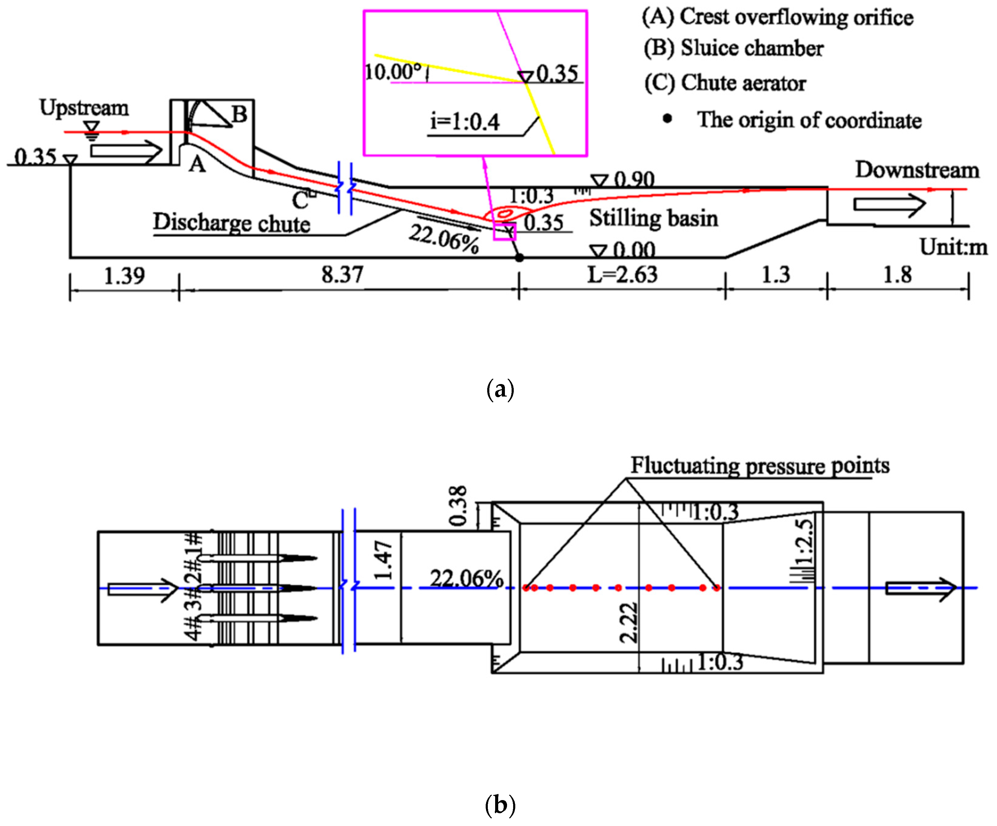
Liyuan Hydropower Station in the Jinsha River, Yunnan Province, China, was physically modeled in the hydraulic laboratory of Northwest Agricultural and Forestry University at a scale of 1:50. As shown in Figure 1, from an economic perspective, the width of the stilling basin should be designed wider than the discharge chute. So the width of the discharge chute and the stilling basin is 147 and 222 cm, respectively, with an expansion ratio of 222/147 = 1.5; the height of bottom drop is 35 cm. Apart from the model layout in Figure 2, it is obvious that the conjunction between the discharge chute and the stilling basin is designed to be expanded abruptly. To avoid redundancy, only 3 operating conditions given in Table 1 are included in this study.
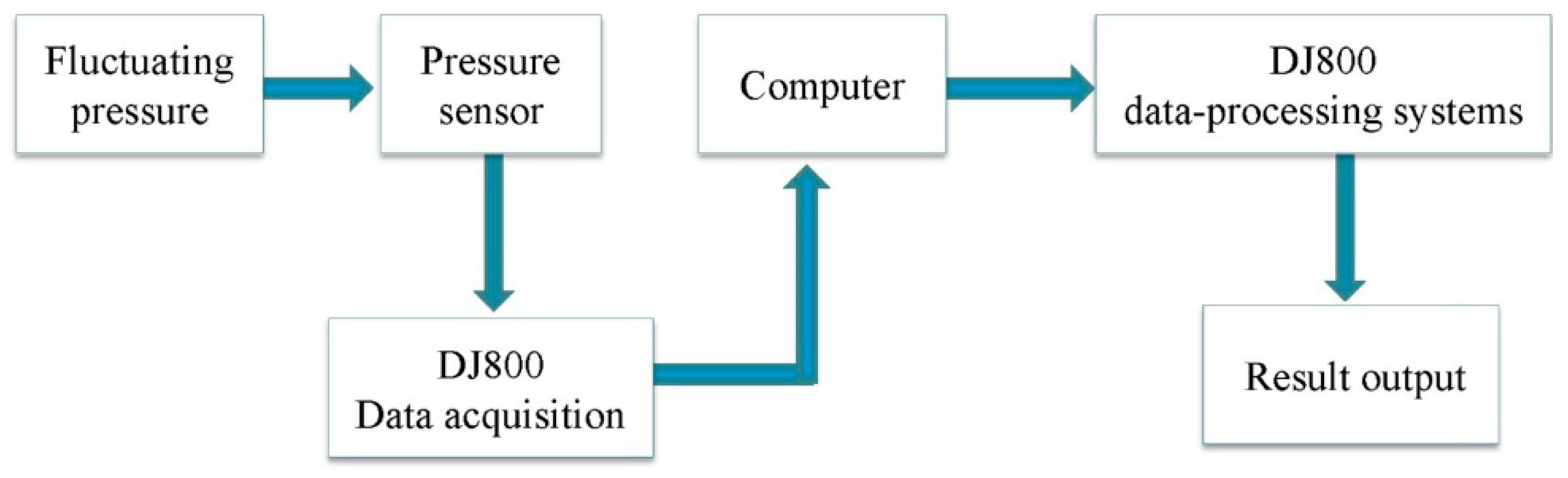
Water was fed to a reservoir by a regulated pump, and the pump rotation speed and the water level in the tank feeding the experimental device remained constant for every measurement. This provided constant discharge, steady flow and boundary conditions to guarantee the repeatability of the experiments. The flow discharge was measured by a rectangular thin-wall weir set up downstream. The velocity was measured by a propeller-type current meter (relative error ≤ ±5%). The data of fluctuating pressure were collected by a DJ800 system, which was developed by the China Institute of Water Resources and Hydropower. The sensor type was selected as piezoresistive silicon pressure transducer (precision: 10 Pa; measurement error: ≤ ±0.5%) to measure time-average and fluctuating pressure. The fluctuating pressure sensor is flush and perpendicular to the pressure measuring surface. After the model manufacturing and installation are completed, inspection, calibration and verification are carried out to reduce errors. The fluctuating pressure data-processing process is shown in Figure 3.
According to previous research results and existing test data, the main frequency of fluctuating pressure is generally concentrated below 25 Hz [25]. According to the requirement of Nyquist sampling theory, the sampling frequency in this test was 50 Hz, which is twice the highest frequency, and the sample capacity was 4096. Data collection at time intervals of 0.02 and 0.04 s was performed in the same working conditions. The statistical analysis results of the collected data show that the RMS value and main frequency of fluctuating pressure at the same measuring points are basically the same at 2 collection frequencies. According to relevant research results and instrument storage capacity, the sample capacity selected was 4096.
2.2. Large Eddy Simulation (LES) Model
In a large eddy simulation (LES) [26,27], the basic idea is to decompose the instantaneous fluctuation motion in turbulence into 2 parts, large-scale and small-scale eddies, through the filtering method, and the large-scale vortex of turbulence is simulated directly by solving the momentum equation, but not directly calculating small-scale vortices, which are represented by a subgrid model. After filtering with the incompressible Navier–Stokes (N-S) equation, the governing equations of the large eddy simulation are obtained:
where u is velocity; t is time; x is the coordinate; i, j is the coordinate orientation; in , the value with “–” represents the large-scale parameters after filtering; is the density of water; g is the acceleration of gravity; μ is the viscosity coefficient; and is the subgrid-scale stress, describing the impact caused by small-eddy movement on large-eddy movement.
The Smagorinsky–Lilly subgrid model is adopted in this paper, and the subgrid stress is computed from
where the turbulent viscosity is molded by
and represents the strain rate tensor, which is defined as
where , , and represents the Smagorinsky constant, which is 0.16 in this study.
FLOW-3D computational fluid dynamics (CFD) software was used in the study. The governing equations involved in this calculation were the continuity, N-S, gas–liquid interface, and turbulence equations. The finite-difference discrete method was used to solve the control equations. The TruVOF method was used to trace the free surface for 3D complicated flow field [28]. The transportation equation of the fluid volume function F in FLOW-3D can be described as follows:
The projection-based generalized minimum residual (GMRES) method was used for the pressure iteration term to improve the solution convergence speed. The Courant–Friedrichs–Lewy maximum number was set to 0.45 [15].
To prevent the solver from diverging at the beginning of the calculation, the initial step size was set to 10−8 s. According to the sampling theorem, the sampling interval time was 0.02 s. Consequently, the total calculation completion time was set to 52.5 s. After the calculation was stable, the simulation time was 30–50.48 s for analysis. In order to analyze the fluctuating pressure in the time domain, the total sampling time was 20.48 s, and 1024 sets of discrete fluctuating pressure data points were accumulated.
2.3. Computational Domain and Boundary Conditions
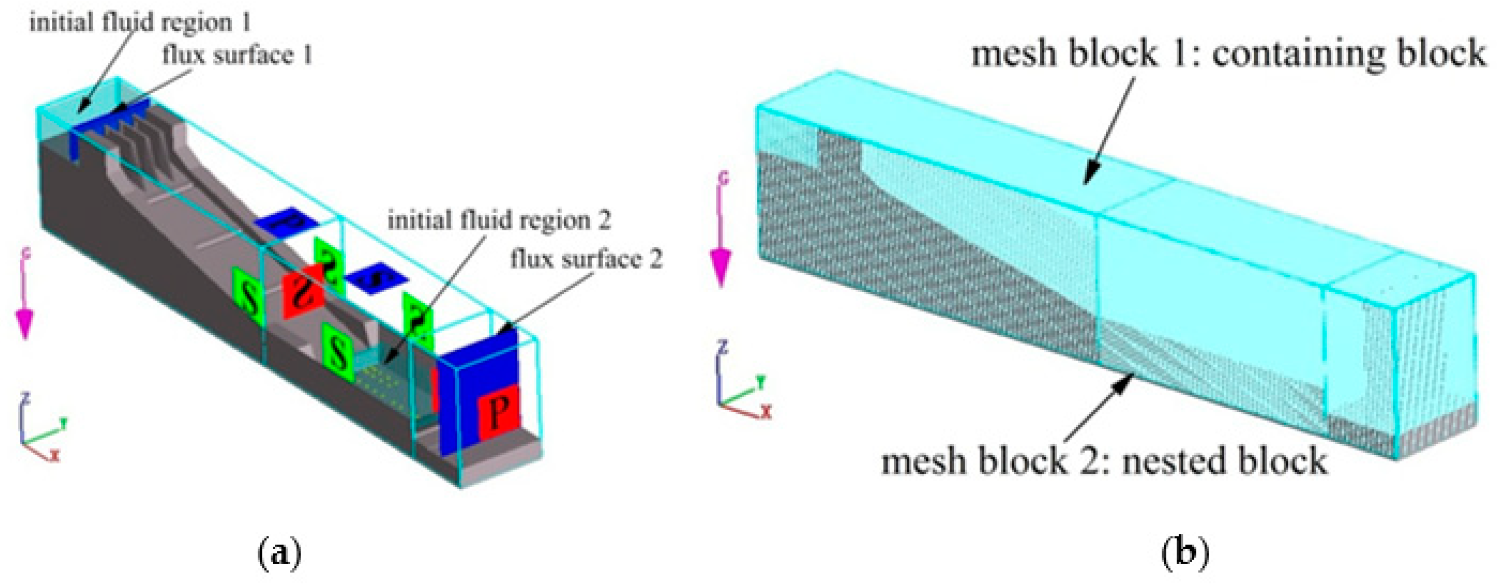
Ten pressure monitoring points were added in the numerical model. The layout of pressure measurement points is shown in Figure 1. The data information sampling interval was consistent with the numerical simulation. The specified pressure P was considered as the inlet of block 1. For the outlet of block 2, the downstream boundary condition adopted a pressure outlet P and the bottom plate of the downstream tailwater section of the stilling basin was used as a reference, and the pressure head was determined according to the model test measurement. Moreover, the specified pressure boundary condition P (P = 0) was considered as the top surface of block 1, which is consistent with atmospheric pressure. For the sides and bottom, the no slip boundary condition S was considered. The wall surface function method was used for the near wall surface, and the wall surface equivalent roughness of the side wall of the sink and the bottom of the stilling basin was taken as 0.001 m. To improve the efficiency of calculation and ensure faster stability, as shown in Figure 4a, two initial water regions as incompressible fluid were added to the numerical model.
3. Numerical Methodology and Model Validation
Combined with the physical model test, the numerical simulation results of representative operating condition 1 were verified and analyzed. The relevant verification results are as follows.
3.1. Grid Sensitivity Analysis
The calculation model has two mesh blocks that use a structured rectangular hexahedral mesh, as shown in Figure 4b. The mesh size of containing block 1 included the entire computational spatial domain, then block 2 was built by a nested grid, which was created for the end of the discharge chute and the stilling basin area where the hydraulic jump took place.
It is well known that simulation results are sensitive to the grid size, especially for LES. Motivated by this, the sensitivity analysis of grid size and quality were studied [29,30]. By adding two flux surfaces to the 3D mathematical model, the discharge of the spillway can be monitored. Typical operating condition 1 was selected for a grid independence test. Four schemes are given in Table 2; it is clear that grids 3 and 4 are sufficient for grid accuracy, the difference of which is 1.49 and 1.06% (<2%), respectively, compared with the physical model results. In order to improve calculation efficiency and ensure computation accuracy, this paper finally adopted grid 3 to carry out a series of simulation studies.
3.2. Comparison of Flow Pattern, Water Surface Profile, and Velocity
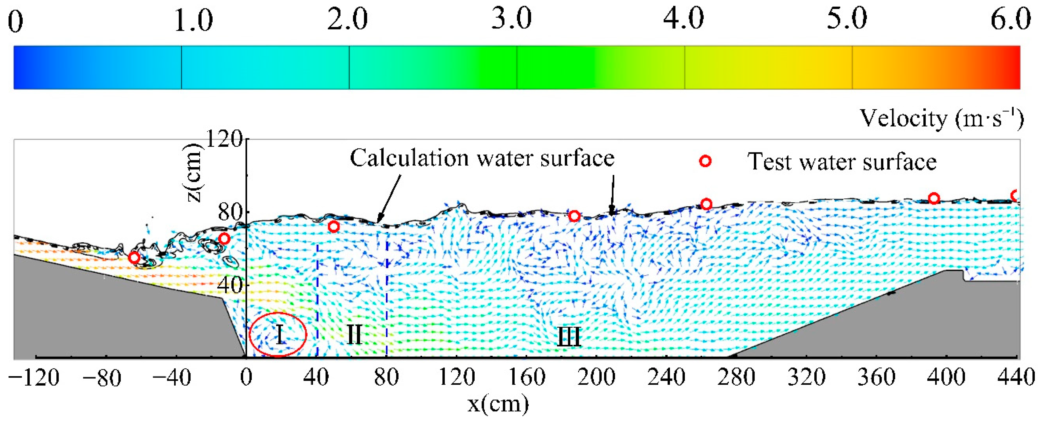
In order to study the hydraulic characteristics on the bottom of the stilling basin slab systematically, the origin of the coordinate was located at the connection between the drop and the center line of the slab. X represents the distance from the measuring point to the drop, Y axis is perpendicular to X at the horizontal plane of the slab, Z represents the distance from the measuring point to the slab along the vertical water depth.
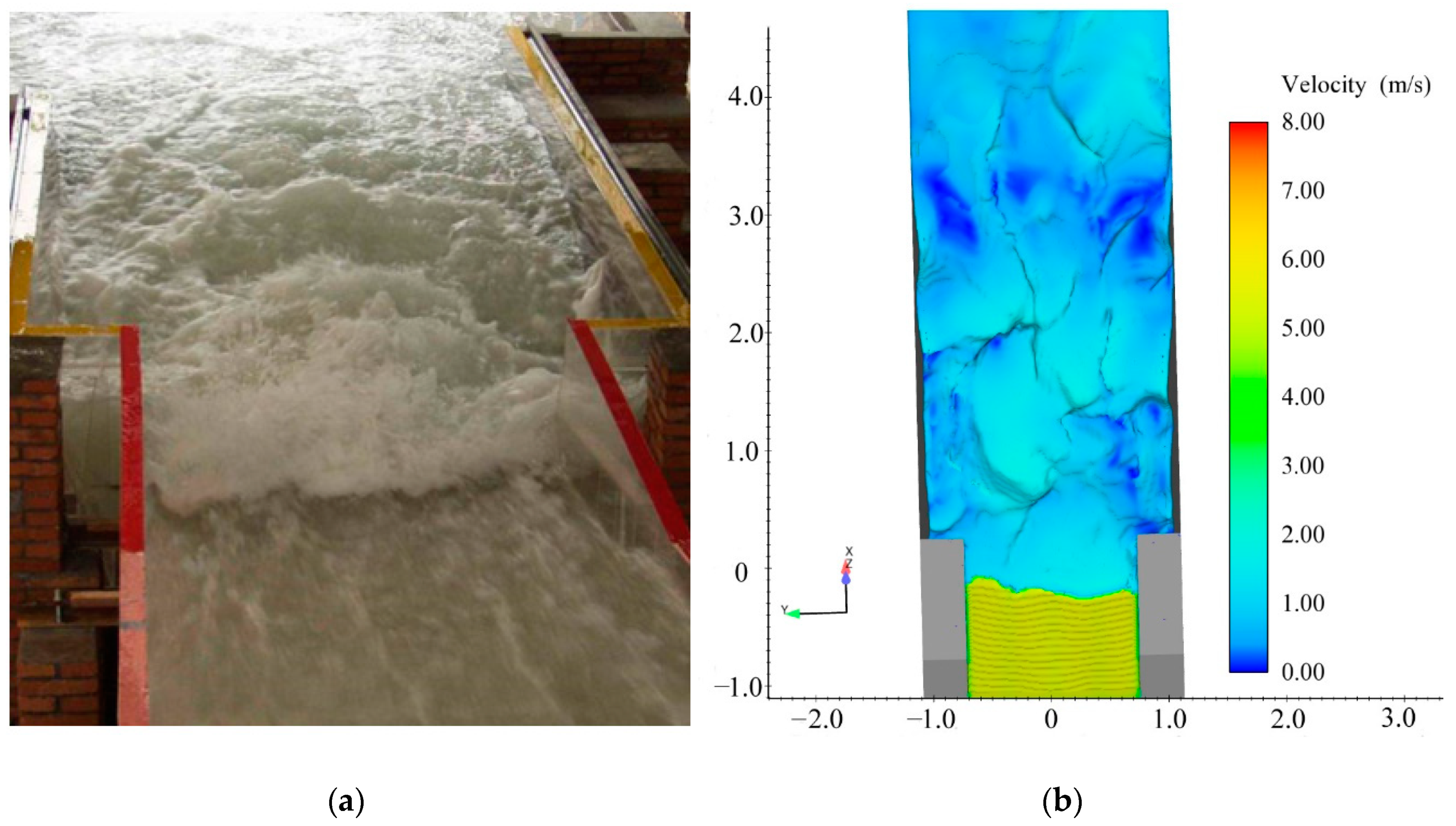
The model test and numerical simulation of the flow patterns are shown in Figure 5. It can be found in the figure that the flow pattern of the LES result is basically consistent with the flow pattern of the physical model test, and the simulation result reflects the severe fluctuation of the water surface in the hydraulic jump region. The distribution along the water surface profile of the stilling basin center line is shown in Figure 6. The discharge channel and stilling basin are connected by vertical expansion and falling drop. The first region of hydraulic jump always occurs at the connection part of the discharge channel and the stilling basin under series unit width discharge. The water surface profile began to rise before the slam, and the peak point was basically in the middle and rear of the stilling basin, that is, the peak point of the hydraulic jump appeared in the stilling basin.
When jets flow into the stilling basin, there are various shapes of eddies with horizontal and vertical vortices. According to previous research [5], this study divided the center line of the stilling basin slab into three zones along the mainstream direction: underflow swirling zone (I), impinging zone (II), and wall-attached jet zone (III). Combined with Figure 4, it can be concluded that because the sluice and the bottom plate are connected by a falling drop, there is a certain thickness of water cushion in the downstream of the stilling basin.
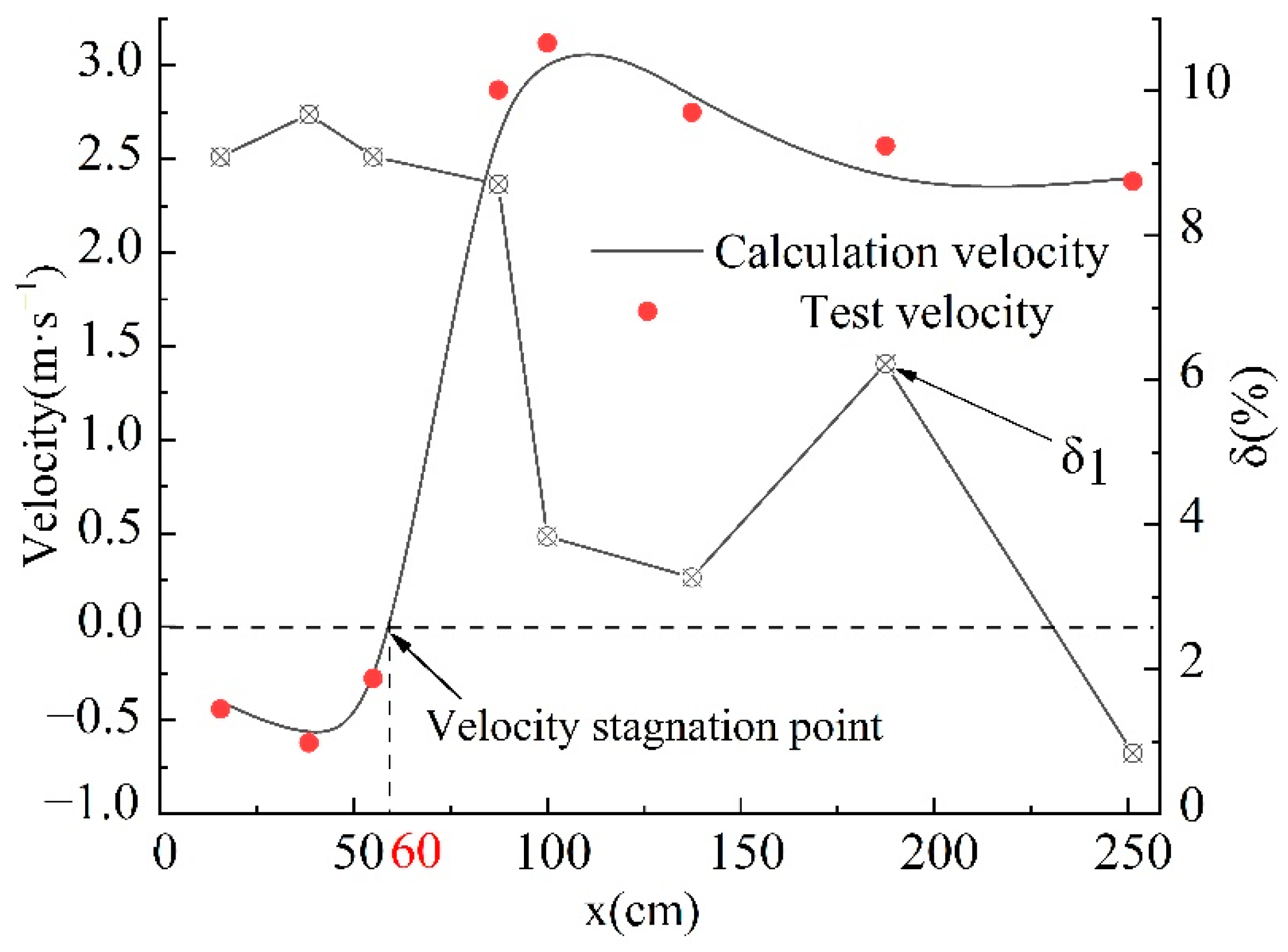
The bottom velocity is an important control parameter for the design of the stilling basin. The relative error of bottom velocity defined as
where VC represents calculation velocity and VT represents test velocity.
The comparison result of bottom velocity is shown in Figure 7, where x is the distance from the measuring points of bottom velocity to the origin of coordinate. The values of x are 15.7 cm, 38.5 cm, 55.1 cm, 87.4 cm, 100.0 cm, 137.4 cm, 187.4 cm, and 251.2 cm. Due to strong turbulence and aeration in the front of the stilling basin, there are some slight differences between the experimental and simulated values of the water surface line and bottom velocity ( < 10%), but the overall trend remains the same.
In the impinging zone (II), there is a velocity stagnation point (Velocity = 0) at x = 60 cm. While the water flows into the stilling basin, the downstream flow gradually descends along the way, forming a horizontal vortex at the bottom of the submerged jet zone. At the same time, due to the influence of the horizontal vortex, the velocity gradient is large, causing an underflow swirling zone in the front of the stilling basin. The flow velocity in zone (I) is negative because of the horizontal clockwise vortex with an elliptical shape underneath the main jets, and the flow velocity of the wall-attached jet zone in the middle and rear part changes smoothly.
In summary, LES can basically reflect the characteristics of the flow field.
3.3. Verification of Pressure
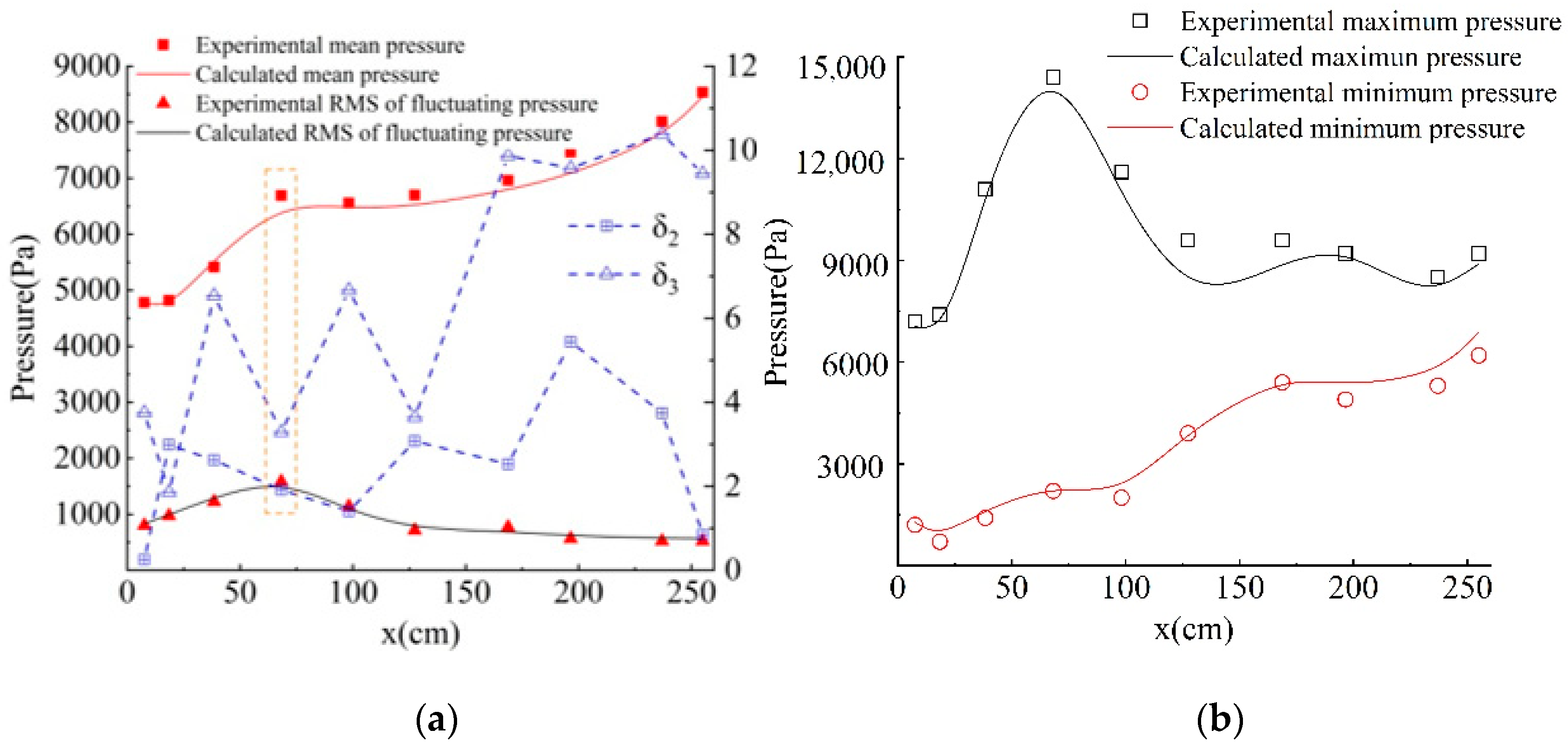
The root mean square (RMS) of the fluctuating pressure (defined as σ) is an important amplitude index to measure the random process of the fluctuating pressure of water flow [31]. The magnitude of σ reflects the degree of violent pressure fluctuation. The time-average pressure and the distribution of σ at 10 pressure measurement points along the center line of the bottom of the stilling basin obtained from the experimental and numerical results are compared. The comparison results are shown in Figure 8a. Solid and hollow points represent experimental and calculated data, respectively, and , represent the relative error of time-average pressure and σ, respectively. The relative error of σ at the rear of the stilling slab is slightly larger ( ≤ 10%) because the water flow was relatively stable. The result shows that the experimental values of time-average pressure and RMS of fluctuating pressure are in good agreement with the simulated values. This indicates that the large eddy model can better simulate time-average and fluctuating pressure on the stilling basin slab. In the impinging zone (II), the main flow of the submerged jet impacted the bottom of the stilling basin, so the time-average hydrodynamic pressure acting on the bottom of the stilling basin slab (II) increased sharply. In the underflow swirling zone, the RMS of fluctuating pressure increased along the way. The pressure at the 4th measuring point (x = 68.3 cm) reached the maximum value and then gradually decreased and remained stable. Both fluctuating and maximum time-average pressure occurred at the 4th measuring point. The comparison of RMS of maximum and minimum pressure is shown in Figure 8b. The calculated maximum pressure is slightly smaller than the experimental maximum pressure. However, the minimum pressure result is the opposite. The reason for this phenomenon is that actual water current fluctuates more sharply.
In summary, with the help of FLOW-3D software, the parameters of time-average pressure, root mean square (RMS) of fluctuating pressure, maximum and minimum pressure of a stilling basin slab by LES are basically consistent with the measured results of the model test. The results demonstrate that the calculation method using the LES model to study the fluctuating pressure of a stilling basin is credible and reasonable.
4. Results and Discussion
4.1. Qualitative Analysis of RMS of Fluctuating Pressure
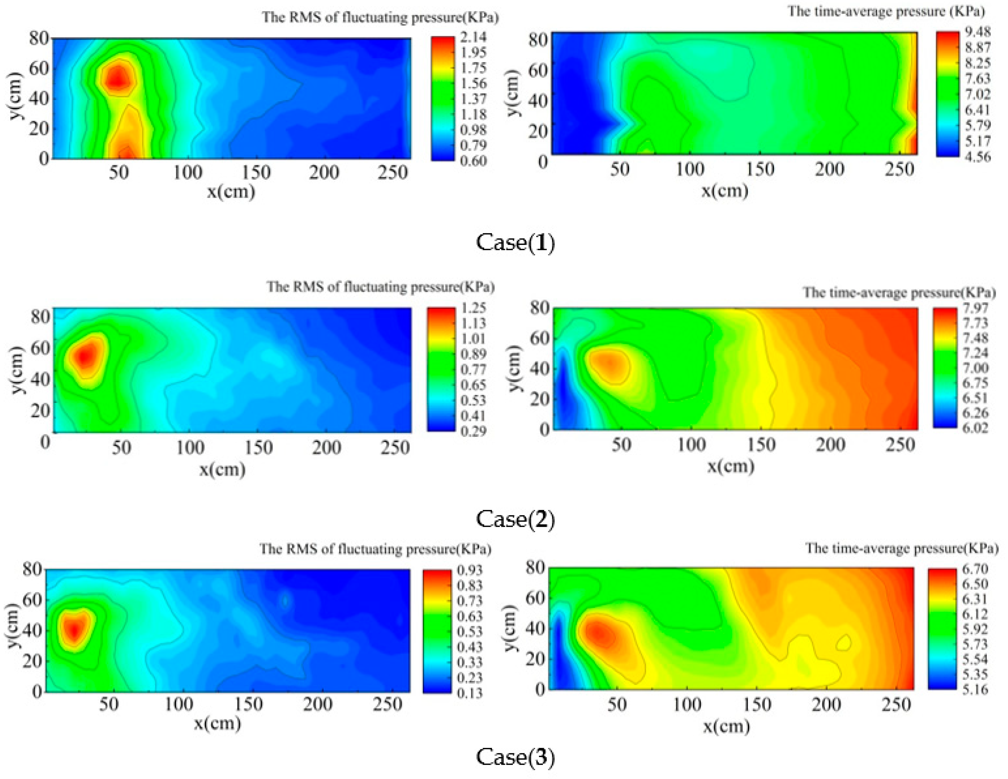
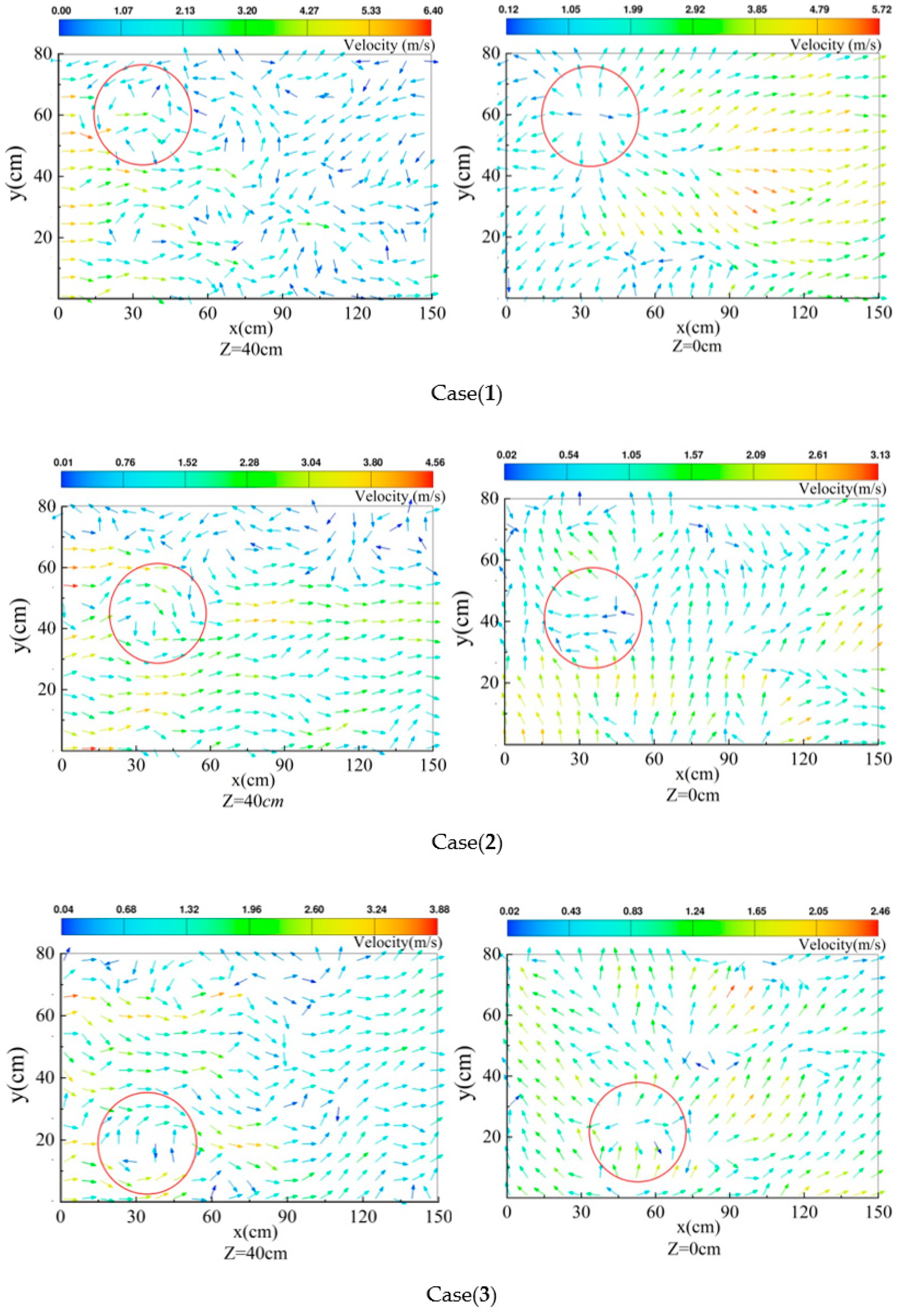
Figure 9 is a distribution diagram of the time-average pressure and σ on the stilling basin slab under three operating conditions. Figure 10 is the vector diagram at the z = 40 cm level and the horizontal plane (z = 0 cm) of the bottom of the stilling basin under the three operating conditions. In Figure 9 and Figure 10, the end of the drop is set as x = 0 cm, the direction of water flow is set as the positive direction of the x-axis, and the front of the end sill x = 263 cm is used as the endpoint coordinates. Since the stilling basin is an axisymmetric structure, its center line is recorded as y = 0 cm, and the endpoint coordinate y = 80 cm at the position offset from the center line to the left by 80 cm. In Figure 9, the fluctuating data was extracted for graphing. Cases 1–3 represent three operating conditions given in Table 1. In case 1, the inflow Froude number (Fr = 5.295) and flow discharge (Q = 0.942 m3/s in physical model, Q = 16,652 m3/s in prototype) is the largest of three working conditions.
4.1.1. Qualitative Analysis of Longitudinal Distribution
Comparing three operating conditions in combination with Figure 9, it can be concluded that the time-average pressure and RMS of fluctuating pressure in the longitudinal direction along the x-axis are relatively small at the front of the stilling basin, and the turbulence of the water flow is very severe due to the presence of the horizontal vortex [18]. At the end of the swirling zone (I) and impinging zone (II), the RMS value gradually increases and reaches the peak value. In the stilling basin, the bottom velocity decreases and its distribution is more uniform. Therefore, the RMS value of fluctuating pressure gradually decreases and tends to be low. Results indicated that fluctuating pressure increase with x/Ls (Ls = stilling basin length), when it reaches the highest point, comes down. Near the sill, the water depth increases and the time-average pressure increases gradually along the way, according to the distribution of hydrostatic pressure. Because the residual flow of water has a certain impact on the tail sill of the stilling basin, the RMS value at the end of the stilling basin increases slightly, and the value of RMS value increases, with decreasing inflow Froude number, which is clearly similar to the experimental results of Yan et al. [25].
4.1.2. Qualitative Analysis of Horizontal Distribution
Due to the sudden lateral enlargement, the main flow of the water is diffused rapidly. When part of the water flows through the bottom drop, a horizontal axis vortex is formed near the bottom drop. Only the remaining part of the flow depends on the downstream water depth to form an incomplete spatial hydraulic jump. Owing to the entrainment effect, two larger vertical vortices and other large and small vertical vortices that are free in a certain area are formed on both sides of the originally incomplete binary 3D hydraulic jump. The existence of multiple vortices expands the turbulence range of the water flow. The turbulence in this area is very strong and the water flow can be quickly dissipated, which improves the energy dissipation rate of the stilling basin to a certain extent. However, the lateral expansion amplitude is relatively small, especially the underwater lateral expansion vertical axis vortex, which is squeezed by the water flow near the side wall, and the rolling strength is difficult to expand horizontally. The superimposed horizontal axis vortex that develops upstream greatly increases the turbulence of the stilling basin slab, which leads to the peak of the RMS value in the area between extension line of the side wall of the vent and x = 25–75 cm. Therefore, the RMS value in the front and middle part of the stilling basin first increases and then decreases from the center line of the bottom to the side wall.
At the same time, in the impinging zone of the stilling basin, the hydrodynamic pressure of the current impact is greater. For the area with a large RMS value of fluctuating pressure, the maximum area is closer to the upstream than the time-average pressure. The main reason is that the vertical axis vortex center is closer to the upstream, due to the superposition of the horizontal and vertical axis vortices, so the area has a large flow velocity gradient. The rotation of the vortex body produces a vertical force on the bottom slab, causing the dynamic water pressure to be stronger than the time-average pressure, so the intensity of fluctuating pressure is larger.
4.1.3. RMS of Fluctuating Pressure Distribution at Different Flow Rates
Combining Figure 9 and Figure 10, the maximum RMS value of fluctuating pressure (denoted as σmax) and the location of occurrence under three operating conditions are given in Table 3.
It can be concluded from the table that operating condition 1 has the largest water flow fluctuation intensity, and the position of the maximum value point occurs the farthest from the center line. The velocity distribution can reflect the flow state of the water flow and further affect the pressure distribution. The distribution of σ is related to the flow field. Combining this with the position distribution of the macro vortex given in Figure 10, it can be obtained that due to the sudden expansion, the water jet entrains to form a vertical axis vortex. With the increases flow discharge, the velocity of the main flow into the stilling basin increases, which causes the centrifugal force of the water flow and the strength of the vortex to increase. The vortex centers move toward the side wall line. In case 3, the flow rate and energy are relatively small, the center of the vertical vortex deviates from the center line to a small degree, and the bottom velocity of the stilling basin is low. On account of the vertical axis vortex being truncated by the horizontal axis vortex, the energy and intensity will also weaken and develop downward, so the RMS of fluctuating pressure is smaller and closer to the center line.
Near the slab of the stilling basin in case 1, there is a vertical vortex structure by water flow, which indicate that the vertical vortex has already reached the slab of the stilling basin. When the location of this vertical vortex is fixed, the intensity of the vortex structure has large effect on the distribution of fluctuating pressure. However, for a stilling basin of multi-horizontal submerged jets(MHSJs),the vertical vortex breaks into subsidiary vortices during the transfer process and moves gradually downstream by Zhang et al. [18]. The intensity of the vortex structure has little effect on slab of the stilling basin.
4.2. Quantitative Analysis of Fluctuating Pressure
4.2.1. Mathematical Model
In the above study, a preliminary qualitative analysis of the distribution of RMS caused by the macro-vortex was carried out. However, the generation mechanism of fluctuating pressure is a very complicated problem. The quantitative analysis requires in-depth research on the generation mechanism of fluctuating pressure.
The Poisson Equation of fluctuating pressure in flow field is as follows [31]:
where and are fluctuating pressure and velocity, respectively, and is time-averaged velocity.
Equation (8) can be considered as the basic governing equation, in which it is clearly indicated that fluctuating pressure is mainly caused by fluctuating velocity. The first item on the right side contains the effect of time-averaged velocity gradient in addition to the effect of fluctuating velocity. The velocity gradient represents the effect of time-averaged shear force, which is called turbulence–shear [32]. This item represents the generation of fluctuating pressure and the combined effect of time-averaged velocity gradient and fluctuating velocity, which is generally called a quick response term. The second term on the right side of Equation (8) only contains the effect of fluctuating velocity itself, known as turbulence–turbulence. According to the two terms in the equation, it can be understood that the generation of fluctuating pressure is composed of two comprehensive factors: the interaction of turbulence–shear and of turbulence–turbulence.
To illustrate the relationship between fluctuating pressure and turbulent vorticity, the turbulent vorticity equation is given as follows:
Substituting Equation (9) into Equation (8), we get:
where , represent turbulence dissipation rate, defined as follows:
The first term on the right side is the quick response term of the time-averaged flow field and the second term is caused by the turbulent vorticity, which reflects the large-scale vortex with concentrated vorticity in the turbulent flow. The third term is caused by the dissipative effect of small-scale vortices, which makes a major contribution to the high-frequency part of the fluctuating pressure. Because the study of turbulent fluctuating pressure is mainly focused on low frequency, the third term can be omitted.
Therefore, by omitting the third item, we finally get:
It can be seen from Equation (12) that the low-frequency and large-amplitude components of turbulent fluctuating pressure are mainly caused by the fast response term in the time-average velocity field and the nonlinear term of the fluctuating velocity field itself caused by the large-scale vortex. It can also be understood that the fluctuating pressure in turbulent flow is the result of the combined action of the flow field and the vorticity field. Governing Equation (12) shows that fluctuating pressure mainly comes from three parameters: fluctuating velocity, flow velocity gradient, and vorticity fluctuation. The first term is the combined effect of fluctuating flow velocity and velocity gradient, and the second term is the effect of vorticity itself. In this case, the combination of fluctuating flow velocity and flow velocity gradient is taken as influencing factor 1, and the vorticity itself is taken as influencing factor 2.
4.2.2. Quantitative Analysis of Longitudinal Distribution
To avoid redundancy, this paper only analyzes the experimental results of representative operating condition 1. We extract the pressure, flow velocity, and vorticity sequence calculated in representative operating condition 1 and RMS processing to get Figure 11.
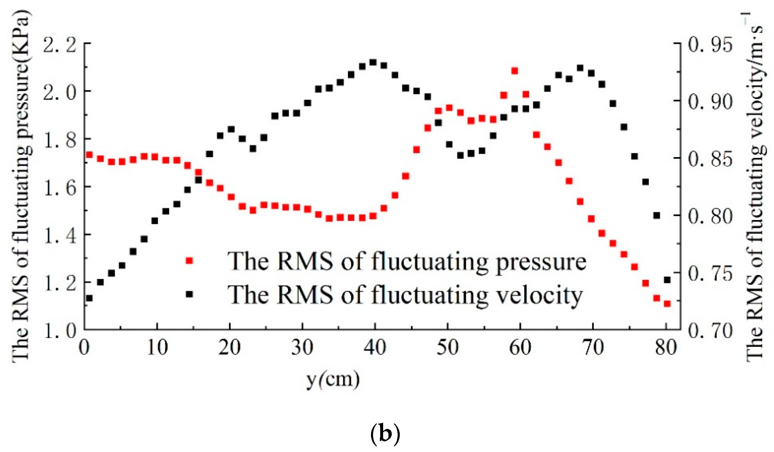
From Figure 11a, it can be found that the RMS of fluctuating pressure in the back section of the stilling basin (x = 100–263 cm) is basically consistent with the RMS of fluctuating velocity, indicating that the fluctuating pressure in the wall-attached jet zone is mainly caused by flow velocity fluctuation. However, there is no correlation in the region of x = 0–100 cm, which reflects that the water flow in the middle of the stilling basin is violently turbulent and the fluctuating velocity is not the main factor causing the fluctuating pressure.
Based on the analysis of Figure 11, it is not difficult to find that in the front of the stilling basin, x = 0–60 cm, there is a good correlation between the RMS values of fluctuating pressure and fluctuating vorticity, mainly due to a large reverse vortex at the bottom of the submerged jet area, and the fluctuating pressure in this area is mainly caused by the vortex. In the stilling basin slab x = 60–100 cm area, the fluctuating pressure is not caused solely by fluctuating velocity or vorticity. The turbulent flow in this area is severe. Moreover, there is also water swirling, which is caused by the combined action of factor 1 (fluctuating velocity and velocity gradient) and factor 2 (fluctuating vorticity).
4.2.3. Cross-Sectional Distribution Quantitative Analysis
In the above analysis, the maximum value of σ in the typical operating condition 1 is near x = 50 cm, so the cross-section at x = 50 cm of the bottom of the stilling basin is cancelled, and the fluctuating pressure distribution is shown in Figure 12.
Comparing Figure 12a,b, the overall trend of the distribution of fluctuating pressure and fluctuating vorticity at this section is basically the same, while fluctuating pressure and fluctuating flow velocity show different distribution trends, with obvious differences in some areas. In the study of the longitudinal distribution law, it was found that x = 0–60 cm was mainly affected by the vortex, and the analysis results here were demonstrated. Especially in the interval of y = 45–80 cm, the degree of correlation with fluctuating vorticity is relatively high. The ordinate of the σmax point of the stilling basin is y = 60 cm, which is located in the core area of the vertical vortex. The distribution of fluctuating pressure is mainly affected by the vorticity. Therefore, quantitative analysis of the RMS distribution law of fluctuating pressure on the stilling basin slab with sudden lateral enlargement and bottom drop needs to be comprehensively considered with multiple influencing factors. The difference of flow patterns in different regions will inevitably affect the distribution of fluctuating pressure.
4.3. Discussion
In this numerical study, hydrodynamic parameters were calculated and analyzed for understanding the fluctuating pressure in the stilling basin with sudden lateral enlargement and bottom drop. The fluctuating pressure coefficient (defined as ) is the most significant parameter among the characteristic parameters of the pressure fluctuation amplitudes and it follows as:
where is the inflow velocity and g is the acceleration of gravity.
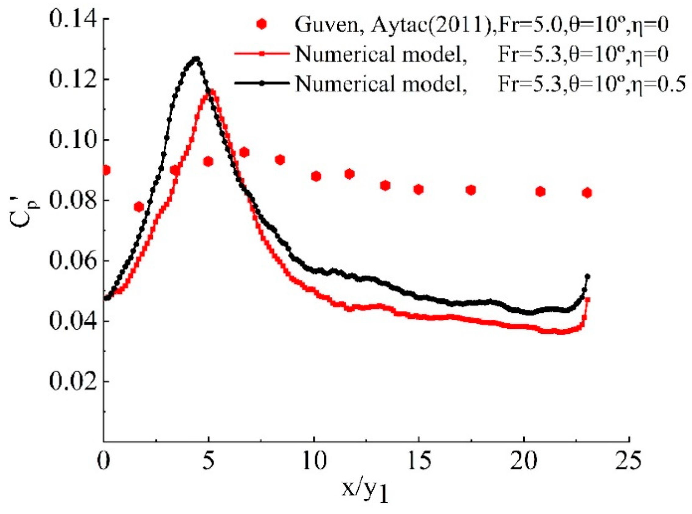
Figure 13 displays the distribution of against x/y1 (y1 is the inflow water depth entering the jump, θ is the angle of entering flow) along with horizontal slab of stilling basin for different inlet Froude number of 5.0 [33] and 5.3 (numerical model in this research). The pressure fluctuation beneath free jump in the spillway with the entering flow at an angle of 10° has been subject to several experimental researches by Gunal. In Figure 13, η = 0 represents the center line of the stilling basin slab, and η = 0.5 represents the half of slab width direction (y = 40 cm).
According to Figure 13, the maximum fluctuating pressure coefficient is located at the beginning of the stilling basin (x/y1 = 0) due to the high turbulence intensity formed by hydraulic jump. In Figure 13, it is observed that fluctuating pressure coefficient first tends to decrease in the range 0 < x/y1 < 2.5, then increases gradually. For the stilling basin with bottom drop, can reach the maximum value at the position of about 5.0 < x/y1 < 6.5 within the impinging zone (II). The results are in accordance with by Yan et al. [25]. and Naseri et al. [21].
If a comparison is made between the maximum values of at two values of η, the maximum difference in fluctuating pressure coefficient is about 10%. Compared with Figure 9 and Figure 13, it was found that the effect of the sudden lateral enlargement on the distribution of fluctuating pressure is considerable.
The varying laws of show that compared to the corresponding classical jumps, the fluctuating pressure characteristics of spatial hydraulic jumps are more complicated. Both sudden lateral enlargement and bottom drop will result in the difference distributions of spatial hydraulic jumps compared with those of equivalent classical hydraulic jumps. Whereas few considerations are provided concerning the effect of different expansion ratios on horizontal distribution of fluctuating pressure coefficient.
5. Conclusions
In this paper, the fluctuating pressure characteristics of a stilling basin slab with sudden lateral enlargement and bottom drop were simulated based on FLOW-3D software and large eddy simulation. Through analysis compared with physical test results, the following conclusions can be drawn:
- The flow pattern, velocity distribution, time-average pressure, root mean square (RMS) of fluctuating pressure, maximum and minimum pressure of a stilling basin slab of the water flow obtained by numerical simulation are in good agreement with the experimental results, indicating that it is advisable to use large eddy simulation to study the fluctuating pressure of stilling basin slab.
- Due to the superposition of the horizontal and vertical vortex, the turbulence and mixing of water in the front of the stilling basin and the extension of the side wall of the vent are severe, resulting in a large RMS of fluctuating pressure in this area, which requires attention. With the increase of per-unit width discharge, the peak point of σ deviates from the center line of the stilling basin and approaches the side wall line. Both sudden lateral enlargement and bottom drop will result in the difference distributions of spatial hydraulic jumps compared with those of equivalent classical hydraulic jumps.
- The RMS of fluctuating pressure longitudinally changes along the center line of the stilling basin, first increasing, then decreasing, and finally increasing slightly. The submerged jet zone is mainly affected by the vortex body, and the impinging zone is affected by the fluctuating velocity and the vortex body. The wall-attached jet zone is mainly caused by the fluctuating velocity. The horizontal direction from the front of the stilling basin along the center to the side wall shows a trend of first decreasing, increasing, and then decreasing, which is highly correlated with the vorticity distribution, but has little correlation with the fluctuating velocity distribution.
Author Contributions
Y.L. carried out the numerical simulation and result analysis as well as writing of the manuscript. J.Y. provided relevant engineering documents and reviewed the manuscript. Z.Y. and K.W. conducted data curation. Z.L. provided relevant fund. All authors contributed to the overall framing and revision of the manuscript at multiple stages. All authors have read and agreed to the published version of the manuscript.
Funding
This research was supported financially by the National Natural Science Foundation of China [Grant No. 51509212].
Informed Consent Statement
Informed consent was obtained from all subjects involved in the study.
Data Availability Statement
All data, models, or code generated or used during the study are available from the corresponding author by request.
Conflicts of Interest
The authors declare no conflict of interest.
References
- Liu, P.Q.; Dong, J.R.; Yu, C. Experimental investigation of fluctuation uplift on rock blocks at the bottom of the scour pool downstream of Three-Gorges spillway. J. Hydraul. Res. 1998, 36, 55–68. [Google Scholar] [CrossRef]
- Liu, P.Q.; Li, A.H. Model discussion of pressure fluctuations propagation within lining slab joints in stilling basins. J. Hydraul. Eng. 2007, 133, 618–624. [Google Scholar] [CrossRef]
- Mousavi, S.N.; Júnior, R.S.; Teixeira, E.D.; Bocchiola, D.; Nabipour, N.; Mosavi, A.; Shamshirband, S. Predictive Modeling the Free Hydraulic Jumps Pressure through Advanced Statistical Methods. Mathematics 2020, 8, 323. [Google Scholar] [CrossRef] [Green Version]
- Sun, S.-K.; Liu, H.-T.; Xia, Q.-F.; Wang, X.-S. Study on stilling basin with step down floor for energy dissipation of hydraulic jump in high dams. J. Hydraul. Eng. 2005, 36, 1188–1193. (In Chinese) [Google Scholar]
- Li, Q.; Li, L.; Liao, H. Study on the Best Depth of Stilling Basin with Shallow-Water Cushion. Water 2018, 10, 1801. [Google Scholar] [CrossRef] [Green Version]
- Luo, Y.-Q.; He, D.-M.; Zhang, S.-C.; Bai, S. Experimental Study on Stilling Basin with Step-down for Floor Slab Stability Characteristics. J. Basic Sci. Eng. 2012, 20, 228–236. (In Chinese) [Google Scholar]
- Zhang, J.; Zhang, Q.; Wang, T.; Li, S.; Diao, Y.; Cheng, M.; Baruch, J. Experimental Study on the Effect of an Expanding Conjunction Between a Spilling Basin and the Downstream Channel on the Height After Jump. Arab. J. Sci. Eng. 2017, 42, 4069–4078. [Google Scholar] [CrossRef]
- Ram, K.V.S.; Prasad, R. Spatial B-jump at sudden channel enlargements with abrupt drop. J. Hydraul. Eng. -Asce 1998, 124, 643–646. [Google Scholar] [CrossRef]
- Hassanpour, N.; Hosseinzadeh Dalir, A.; Farsadizadeh, D.; Gualtieri, C. An Experimental Study of Hydraulic Jump in a Gradually Expanding Rectangular Stilling Basin with Roughened Bed. Water 2017, 9, 945. [Google Scholar] [CrossRef] [Green Version]
- Siuta, T. The impact of deepening the stilling basin on the characteristics of hydraulic jump. Czas. Tech. 2018. [Google Scholar] [CrossRef]
- Babaali, H.; Shamsai, A.; Vosoughifar, H. Computational Modeling of the Hydraulic Jump in the Stilling Basin with Convergence Walls Using CFD Codes. Arab. J. Sci. Eng. 2014, 40, 381–395. [Google Scholar] [CrossRef] [Green Version]
- Dehdar-behbahani, S.; Parsaie, A. Numerical modeling of flow pattern in dam spillway’s guide wall. Case study: Balaroud dam, Iran. Alex. Eng. J. 2016, 55, 467–473. [Google Scholar] [CrossRef] [Green Version]
- Macián-Pérez, J.F.; García-Bartual, R.; Huber, B.; Bayon, A.; Vallés-Morán, F.J. Analysis of the Flow in a Typified USBR II Stilling Basin through a Numerical and Physical Modeling Approach. Water 2020, 12, 227. [Google Scholar] [CrossRef] [Green Version]
- Tajabadi, F.; Jabbari, E.; Sarkardeh, H. Effect of the end sill angle on the hydrodynamic parameters of a stilling basin. Eur. Phys. J. Plus 2018, 133. [Google Scholar] [CrossRef]
- Valero, D.; Bung, D.B.; Crookston, B.M. Energy Dissipation of a Type III Basin under Design and Adverse Conditions for Stepped and Smooth Spillways. J. Hydraul. Eng. 2018, 144. [Google Scholar] [CrossRef]
- Liu, D.; Fei, W.; Wang, X.; Chen, H.; Qi, L. Establishment and application of three-dimensional realistic river terrain in the numerical modeling of flow over spillways. Water Supply 2018, 18, 119–129. [Google Scholar] [CrossRef]
- Epely-Chauvin, G.; De Cesare, G.; Schwindt, S. Numerical Modelling of Plunge Pool Scour Evolution In Non-Cohesive Sediments. Eng. Appl. Comput. Fluid Mech. 2015, 8, 477–487. [Google Scholar] [CrossRef] [Green Version]
- Zhang, J.-M.; Chen, J.-G.; Xu, W.-L.; Peng, Y. Characteristics of vortex structure in multi-horizontal submerged jets stilling basin. Proc. Inst. Civ. Eng. Water Manag. 2014, 167, 322–333. [Google Scholar] [CrossRef]
- Li, L.-X.; Liao, H.-S.; Liu, D.; Jiang, S.-Y. Experimental investigation of the optimization of stilling basin with shallow-water cushion used for low Froude number energy dissipation. J. Hydrodyn. 2015, 27, 522–529. [Google Scholar] [CrossRef]
- Ferreri, G.B.; Nasello, C. Hydraulic jumps at drop and abrupt enlargement in rectangular channel. J. Hydraul. Res. 2010, 40, 491–505. [Google Scholar] [CrossRef]
- Naseri, F.; Sarkardeh, H.; Jabbari, E. Effect of inlet flow condition on hydrodynamic parameters of stilling basins. Acta Mech. 2017, 229, 1415–1428. [Google Scholar] [CrossRef]
- Zhou, Z.; Wang, J.-X. Numerical Modeling of 3D Flow Field among a Compound Stilling Basin. Math. Probl. Eng. 2019, 5934274. [Google Scholar] [CrossRef] [Green Version]
- Qian, Z.; Hu, X.; Huai, W.; Amador, A. Numerical simulation and analysis of water flow over stepped spillways. Sci. China Ser. E Technol. Sci. 2009, 52, 1958–1965. [Google Scholar] [CrossRef]
- Liu, F. Study on Characteristics of Fluctuating Wall-Pressure and Its Similarity Law. Ph.D. Thesis, Tianjin University, Tianjin, China, May 2007. (In Chinese). [Google Scholar]
- Yan, Z.-M.; Zhou, C.-T.; Lu, S.-Q. Pressure fluctuations beneath spatial hydraulic jumps. J. Hydrodyn. 2006, 18, 723–726. [Google Scholar] [CrossRef]
- Moin, P.; Kim, J. Numerical investigation of turbulent channel flow. J. Fluid Mech. 2006, 118. [Google Scholar] [CrossRef] [Green Version]
- Rezaeiravesh, S.; Liefvendahl, M. Effect of grid resolution on large eddy simulation of wall-bounded turbulence. Phys. Fluids 2018, 30. [Google Scholar] [CrossRef] [Green Version]
- Stamou, A.I.; Chapsas, D.G.; Christodoulou, G.C. 3-D numerical modeling of supercritical flow in gradual expansions. J. Hydraul. Res. 2010, 46, 402–409. [Google Scholar] [CrossRef]
- Savage, B.M.; Crookston, B.M.; Paxson, G.S. Physical and Numerical Modeling of Large Headwater Ratios for a 15 degrees Labyrinth Spillway. J. Hydraul. Eng. 2016, 142. [Google Scholar] [CrossRef]
- Aydin, M.C.; Ozturk, M. Verification and validation of a computational fluid dynamics (CFD) model for air entrainment at spillway aerators. Can. J. Civ. Eng. 2009, 36, 826–836. [Google Scholar] [CrossRef] [Green Version]
- Ma, B.; Liang, S.; Liang, C.; Li, Y. Experimental Research on an Improved Slope Protection Structure in the Plunge Pool of a High Dam. Water 2017, 9, 671. [Google Scholar] [CrossRef] [Green Version]
- Bai, L.; Zhou, L.; Han, C.; Zhu, Y.; Shi, W.D. Numerical Study of Pressure Fluctuation and Unsteady Flow in a Centrifugal Pump. Processes 2019, 7, 354. [Google Scholar] [CrossRef] [Green Version]
- Guven, A. A predictive model for pressure fluctuations on sloping channels using support vector machine. Int. J. Numer. Methods Fluids 2011, 66, 1371–1382. [Google Scholar] [CrossRef]
Figure 1.
Schematic design of model test: (a) Sectional view; (b) Plan view.

Figure 2.
Model layout in laboratory: (a) Discharge chute; (b) The stilling basin.

Figure 3.
Schematic diagram of fluctuating pressure data-processing process.

Figure 4.
3D simulation model: (a) Boundary conditions; (b) Grid mesh.

Figure 5.
Flow pattern of operating condition 1: (a) Physical model flow diagram; (b) Simulation model flow.
Figure 5.
Flow pattern of operating condition 1: (a) Physical model flow diagram; (b) Simulation model flow.

Figure 6.
Numerical simulation of water surface profile and x-z plane flow rate vector.

Figure 7.
Comparison of bottom velocity.

Figure 8.
Comparison of pressure at 10 pressure measurement points: (a) Comparison of root mean square (RMS) of fluctuating and time-average pressure; (b) Comparison of maximum and minimum pressure.
Figure 8.
Comparison of pressure at 10 pressure measurement points: (a) Comparison of root mean square (RMS) of fluctuating and time-average pressure; (b) Comparison of maximum and minimum pressure.

Figure 9.
The distribution diagram of time-average pressure and RMS of fluctuating pressure of bottom of stilling basin under three cases.
Figure 9.
The distribution diagram of time-average pressure and RMS of fluctuating pressure of bottom of stilling basin under three cases.

Figure 10.
Speed vector in stilling basin at z = 40 cm horizontal plane and bottom plate plane in three cases.
Figure 10.
Speed vector in stilling basin at z = 40 cm horizontal plane and bottom plate plane in three cases.

Figure 11.
Distribution of fluctuating velocity and vorticity in the horizontal section of the stilling basin slab: (a) Distribution of fluctuating velocity; (b) Distribution of fluctuating vorticity.
Figure 11.
Distribution of fluctuating velocity and vorticity in the horizontal section of the stilling basin slab: (a) Distribution of fluctuating velocity; (b) Distribution of fluctuating vorticity.

Figure 12.
Distribution of root time-average square fluctuating pressure of x = 50 cm cross-section of bottom plate: (a) Distributions of fluctuating velocity and fluctuating pressure; (b) Distributions of fluctuating vorticity and fluctuating pressure.
Figure 12.
Distribution of root time-average square fluctuating pressure of x = 50 cm cross-section of bottom plate: (a) Distributions of fluctuating velocity and fluctuating pressure; (b) Distributions of fluctuating vorticity and fluctuating pressure.


Figure 13.
Variance of fluctuating pressure coefficient ().


Table 1.
Operating conditions.
| Condition | Flow Discharge (m3/s) | Inflow Froude Number | Inflow Velocity (m/s) | Inflow Water Depth (m) |
|---|---|---|---|---|
| 1 | 0.942 | 5.295 | 5.611 | 0.114 |
| 2 | 0.643 | 4.545 | 4.489 | 0.097 |
| 3 | 0.232 | 4.227 | 3.018 | 0.052 |
Table 2.
Grid independence test.
| Grid | Containing Block Cell Size (m) | Nested Block Cell Size (m) | Discharge (m3/s) | Relative Error (%) |
|---|---|---|---|---|
| 1 | 0.050 | 0.025 | 0.990 | 5.10 |
| 2 | 0.040 | 0.020 | 0.969 | 2.70 |
| 3 | 0.030 | 0.015 | 0.956 | 1.49 |
| 4 | 0.020 | 0.010 | 0.952 | 1.06 |
Table 3.
Distribution of σmax points under three operating conditions.
| Condition | σmax (Pa) | σmax Point Coordinates (cm) |
|---|---|---|
| 1 | 2139 | (50,60) |
| 2 | 1253 | (35,55) |
| 3 | 932 | (30,35) |
Publisher’s Note: MDPI stays neutral with regard to jurisdictional claims in published maps and institutional affiliations. |
© 2021 by the authors. Licensee MDPI, Basel, Switzerland. This article is an open access article distributed under the terms and conditions of the Creative Commons Attribution (CC BY) license (http://creativecommons.org/licenses/by/4.0/).
Share and Cite
MDPI and ACS Style
Lu, Y.; Yin, J.; Yang, Z.; Wei, K.; Liu, Z. Numerical Study of Fluctuating Pressure on Stilling Basin Slab with Sudden Lateral Enlargement and Bottom Drop. Water 2021, 13, 238. https://doi.org/10.3390/w13020238
AMA Style
Lu Y, Yin J, Yang Z, Wei K, Liu Z. Numerical Study of Fluctuating Pressure on Stilling Basin Slab with Sudden Lateral Enlargement and Bottom Drop. Water. 2021; 13(2):238. https://doi.org/10.3390/w13020238
Chicago/Turabian StyleLu, Yangliang, Jinbu Yin, Zhou Yang, Kebang Wei, and Zhiming Liu. 2021. "Numerical Study of Fluctuating Pressure on Stilling Basin Slab with Sudden Lateral Enlargement and Bottom Drop" Water 13, no. 2: 238. https://doi.org/10.3390/w13020238
Note that from the first issue of 2016, this journal uses article numbers instead of page numbers. See further details here.