Article

Flood Susceptibility Assessment Using Novel Ensemble of Hyperpipes and Support Vector Regression Algorithms

1
Department of Geography, The University of Burdwan, Bardhaman 713104, West Bengal, India
2
Department of Geomorphology, Tarbiat Modares University, Tehran 14117-13116, Iran
3
Department of Geoinformatics–Z_GIS, University of Salzburg, 5020 Salzburg, Austria
4
Department of Computer Engineering, Faculty of Valiasr, Tehran Branch, Technical and Vocational University (TVU), Tehran 14356-61137, Iran
5
Research Institute of the University of Bucharest, 90–92 Sos. Panduri, 5th District, 050107 Bucharest, Romania
6
National Institute of Hydrology and Water Management, București-Ploiești Road, 97E, 1st District, 013686 Bucharest, Romania
7
University Center for Research & Development (UCRD), Chandigarh University, Mohali 140413, Punjab, India
8
Department of Geography, Faculty of Natural Sciences, Jamia Millia Islamia, New Delhi 110025, Delhi, India
*
Authors to whom correspondence should be addressed.
Water 2021, 13(2), 241; https://doi.org/10.3390/w13020241
Submission received: 8 November 2020 / Revised: 1 January 2021 / Accepted: 3 January 2021 / Published: 19 January 2021
(This article belongs to the Special Issue Flash-Flood Susceptibility, Forecast and Warning)

Abstract

:
Recurrent floods are one of the major global threats among people, particularly in developing countries like India, as this nation has a tropical monsoon type of climate. Therefore, flood susceptibility (FS) mapping is indeed necessary to overcome this type of natural hazard phenomena. With this in mind, we evaluated the prediction performance of FS mapping in the Koiya River basin, Eastern India. The present research work was done through preparation of a sophisticated flood inventory map; eight flood conditioning variables were selected based on the topography and hydro-climatological condition, and by applying the novel ensemble approach of hyperpipes (HP) and support vector regression (SVR) machine learning (ML) algorithms. The ensemble approach of HP-SVR was also compared with the stand-alone ML algorithms of HP and SVR. In relative importance of variables, distance to river was the most dominant factor for flood occurrences followed by rainfall, land use land cover (LULC), and normalized difference vegetation index (NDVI). The validation and accuracy assessment of FS maps was done through five popular statistical methods. The result of accuracy evaluation showed that the ensemble approach is the most optimal model (AUC = 0.915, sensitivity = 0.932, specificity = 0.902, accuracy = 0.928 and Kappa = 0.835) in FS assessment, followed by HP (AUC = 0.885) and SVR (AUC = 0.871).

1. Introduction

Among the several natural disasters, floods are the more frequent and costly, as they lead to massive damage of life and property including biodiversity and ecological degradation through soil losses [1,2,3]. Floods may be defined as the overflowing of river water from its channel course and cause inundation of surrounding areas [4]. Floods are one of the most devastating natural phenomena occurring throughout the world, mainly caused by long period of rainfalls or snowmelt with the amalgamation of other adverse geo-environmental conditions [5]. Recently, occurrences of floods have also been responsible for human interventions in the environment and have been occurring more frequently than before, basically due to the large scale environmental degradation through population growth, river side flood plain encroachment, urbanization, deforestation, and more [6,7]. Research studies have shown that by the end of 2050, more than 1.3 billion people will be living in flood risk areas [8], and experiencing hazardous flooding phenomena. Moreover, changing climatic conditions associated with huge amounts of rainfall within short time periods are also responsible for recurrent occurrence of floods, including flash floods [9,10]. Flood occurrence is seen as a risk when a large group of people is affected by the flood and it is responsible for loss of infrastructure, settlements, and more. Therefore, the frequency of flood risk has been largely impacting on the possible damages of flooding. It is also fact that the damages caused by flooding are not quantifiable in a precise form [11].
The scenario of floods in Asia is also devastating, as more than 90% of destruction is caused on this continent by flood hazards [12]. It is also mentioned here that tropical rivers are the more frequent in the occurrences of flood [13]. Developing countries like India have also noticed frequent flood hazards due to various favorable conditions related to flood occurrences. Studies revealed that India is the most badly flood affected country after Bangladesh [14]. In India, floods that occurred throughout the country in the year of 2000 were the most noteworthy as declared by government of India, as a total of approximately 5560.65 cores of economy were losses along with 2.21 cores people were affected [9]. In 2013, the Central Water Commission (CWC) of India estimated that 7.21 million hectares of land inundated and nearly 32 million people were affected by flooding [15]. Several areas of India are affected by devastating floods, among them Kerala flooding in August 2018 was most damaging as nearly 4.3 and 1.4 million people were affected and displaced, respectively, along with a death toll of 433 people. Moreover, flooding in Assam (2016), Bihar (2020), Mumbai (2005), and Uttrakhand (2013) were severe cases and are the more frequent flood prone areas. In the state of West Bengal, more than 50% of the area has been affected by devastating floods, particularly in the district of Maldah, Murshidabad, Birbhum, and Purba Bardhaman, and these districts are badly affected by flooding every year of various magnitudes and intensities. Therefore, the flood risk phenomena cannot be disregarded, and to mitigate this risk, proper identification and spatial prediction of flood prone areas is necessary through flood susceptibility (FS) mapping by using several methods.
Spatial analysis of environmental assessment has been carried out by using remote sensing (RS) [16,17,18,19,20,21] and geographic information system (GIS) [22,23] tools. Hence, in the last few decades, FS mapping has been carried out through several statistical methods. In recent years, various fuzzy [24,25,26,27,28], deep learning [29,30,31,32,33,34], multiple criteria decision-making (MCDM) [35,36,37], and statistical [38,39,40,41,42,43] models have used by researchers. The most used statistical methods in FS assessment are frequency ratio (FR) [38], analytical hierarchy process (AHP) [39], and more. Thereafter, with the advance of time and to fulfill the lacking of statistical methods, several machine learning (ML) algorithms have been widely used for FS assessment among research groups throughout the world. The frequently used ML algorithms for FS assessment are random forest (RF) [6], support vector machine (SVM) [40], functional tree (FT) [41], evidential belief function (EBF) [42], bio-geography based optimization (BBO) [9], and more. Afterward, the ensemble approach has been evolved to prepare more accurate prediction results of FS assessment. Researchers try to combine two or more statistical or ML algorithms to develop an ensemble approach for better prediction performance analysis. Research studies have shown that ensemble approaches have been more widely used to evaluate FS mapping than any stand-alone ML algorithms. Several ensemble approaches have been used for FS assessment, including ensemble of tree based ML algorithms [6], EBF-LR [42], and more.
In this research, we have chosen a sub-tropical river basin of Koiya River as a study area for FS assessment. Our main research objective is to prepare spatial prediction of FS maps for mitigation and sustainable management of flooding activities. Basically, this type of research study is not based on a specific time period, usually this type of work has analyzed the spatial prediction of flooding and not within a certain time period, until we have considered the climate change phenomena. If we considered prediction of FS under climate change activities, then it should be bounded by certain time period. However, the duration of flood time window (few days to few weeks) has been largely dependent on local geo-environmental factors i.e., duration and intensity of rainfall, percentage of vegetation cover, elevation and more. Thus, to progress in our work on FS assessment, here we have selected a total of eight flood susceptibility conditioning factors (FSCFs) based on the topography and hydro-climatological conditions, and these factors are land use land cover (LULC), soil type, rainfall, normalized difference vegetation index (NDVI), distance to river, elevation, topographic wetness index (TWI), and stream power index (SPI), as these condition have direct or indirect influence on the occurrences of flood. All of these factors are widely responsible for recurrent flooding and the associated risks. An inventory flood map was also prepared based on the historical data of 132 flood points, because an inventory map is the foremost condition for modelling FS assessment. The variables’ importance for occurrences of flood was identified through the random forest (RF) algorithm. The present research work of FS modeling and mapping was carried out by using the two ML algorithms of hyperpipes (HP) and support vector regression (SVR); and the novel ensemble of HP-SVR approach was employed for better analysis of prediction result. Literature study has shown that the HP algorithm was used in landslide susceptibility analysis and several ensemble approaches with HP gave better result than single HP. Thus, the best of our knowledge and intensive studies have shown that the ensemble of HP-SVR has not been used before for FS mapping; therefore, this ensemble approach is the novelty in this research study. The respective model’s output result was validated through five popular statistical indices including receiver operating characteristics (ROC) curve analysis.

2. Materials and Methods

2.1. Study Area

The present research work was carried out in a non-perennial river of Koiya river basin and it is a main tributary of the Mayurakshi River. The frequent occurrences of flood in the Koiya river basin are a very well-known phenomena, particularly during the peak monsoon month. In eastern India, peak monsoon month (maximum rainfall received during this time) generally varies from July to September due to monsoon-dominated climatic characteristics. The Kopai and Bakreshwar River join together to form Koiya River and flow through the Birbhum and Murshidabad districts. The spatial extension of this basin area is from 23°37′41″ N to 23°57′52″ N latitude and 87°16′54″ E to 88°08′50″ E longitude with an aerial coverage of 1433.69 km2. (Figure 1). The entire river basin area is dominated by productive agricultural land, except some portion of the upper course in the basin. The climate in this study area is dominated by tropical monsoon type, and the maximum and minimum temperature ranges from 12 °C to 17 °C and 35° to 40 °C, respectively. Maximum rainfall occurs in the peak monsoon months (July to September) and average annual rainfall varies from 1200 to 1700 mm [42]. Elevation in this study area ranges from 4 to 145 m, therefore lower courses of the basin area are highly flood prone during the rainy monsoon season.

2.2. Methodology

The methodological flow chart of the present research on spatial prediction of FS assessment is shown in Figure 2 and was carried out by following several steps.
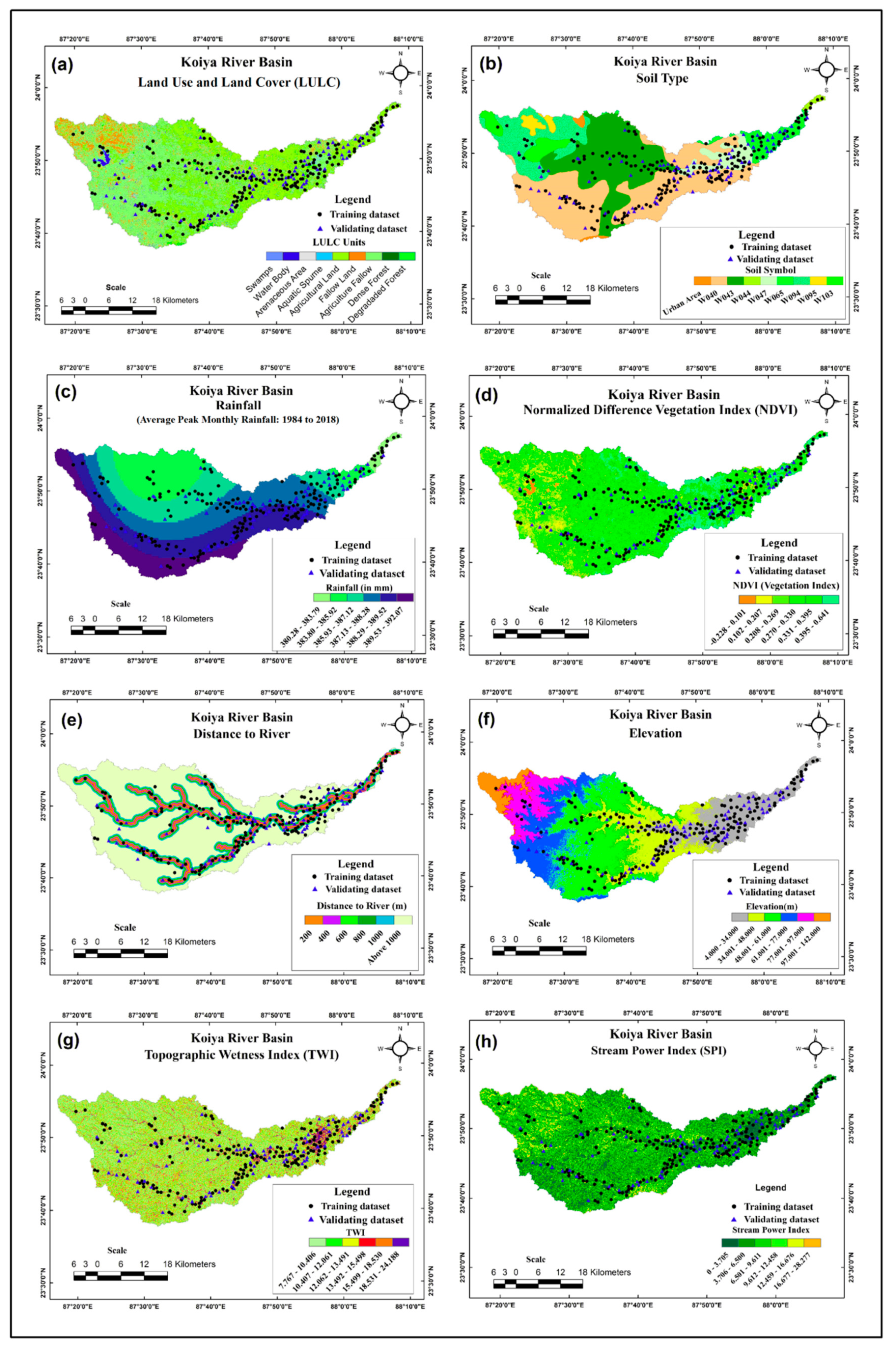
  • Preparation of flood inventory map and several flood susceptibility conditioning factors (FSCFs): a total of 264, in which 132 historical flood points were collected from the multi-hazard district disaster management plan of Birbhum for the two respective year of 2017 and 2018 (http://www.birbhum.gov.in/DMD/MH_DM_Plan_Birbhum) and verified through Google earth satellite images. Alongside this, an extensive field survey was carried out to check flood level marker posts during the flood time. Afterward, 132 non-flood points were randomly selected throughout the river basin area with the help of the ArcGIS platform. Additionally, a total of eight FSCFs were chosen, namely land use land cover (LULC), soil types, rainfall, normalized difference vegetation index (NDVI), distance to river, elevation, topographic wetness index (TWI), and stream power index (SPI) based on the local geo-environmental conditions for further progress of our research work.
  • Multi-collinearity analysis was carried out among the selected factors by using tolerance (TOL) and variance inflation factor (VIF) techniques to reduce the bias.
  • Relative importance of eight variables and their sub-classes was analyzed through the mean decrease accuracy (MDA) method of the random forest (RF) algorithm and step-wise weight assessment ratio analysis (SWARA).
  • Flood susceptibility modeling and mapping was done through hyperpipes (HP), support vector regression (SVR) ML algorithms, and their novel ensemble of HP-SVR.
  • The prediction performance of the aforementioned three models was validated through the statistical methods of sensitivity, specificity, accuracy, receiver operating characteristics-area under curve (ROC-AUC), and Kappa coefficient analysis.

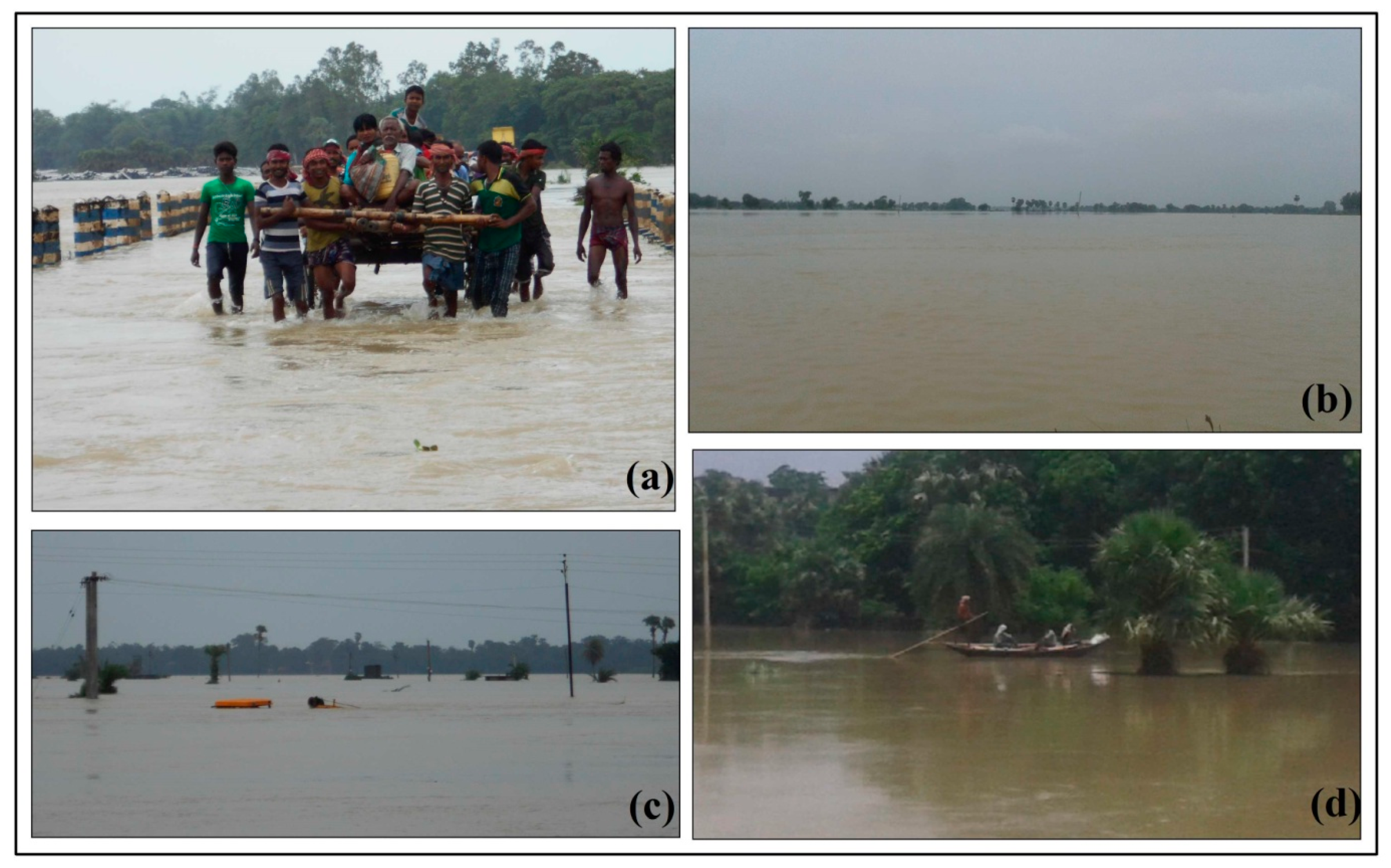
2.3. Flood Inventory Map

In a FS analysis, the surface area can be categorized into two different zones, i.e., sites where floods have already occurred and sites where floods have not occurred but have a possibility of future occurrences. This type of phenomenon has been presented in a flood inventory map. Thus, the preparation of a flood inventory map is the most prerequisite step for flood susceptibility assessment by using historical data of flood occurrences [43]. Past and present flood-induced inundation areas have been presented through flood inventory map within a particular river basin area [44]. It is also a very well-known fact that the utmost accuracy of FS depends on a good flood inventory map. Thus, to estimate the future flood occurrence prone areas, it is indeed necessary to carry out a detailed analysis of the historical flood data [45]. In this study, we have also prepared a flood inventory map (Figure 1). A total of 264 (132 each for flood and non-flood) flood points have been used to do so. We randomly split the entire dataset into 70% (185) and 30% (79) for training and validation purposes, respectively, so that it covered throughout the study area. Historical flood points were collected from multi-hazard district disaster management plan, Birbhum (2017–2018), Google earth satellite image, field survey with a handle GPS (global positioning system) during the time of flood hazard, and by discussing with local people about the intensity of floods. Similarly, non-flood points were incorporated in the inventory map through random selection procedure using ArcGIS 10.4 software. Figure 3 shows some of the ground photographs during the flood time.

2.4. Data Preparation

The most vital step for preparation of a FS map is to choose several appropriate FSCFs. In general, FSCFs have been selected based on local geo-environmental factors, thus region-to-region occurrences of flood conditioning factors have also been varied accordingly [46]. Several research works have been done on FS analysis by using various factors like geological (tectonic), climatological, hydrological, geomorphological, and human interventions [19]. Therefore, keeping in view the above fact, we have also chosen eight appropriate FSCFs in this study, based on the previous literature survey and local geo-environmental conditions. These factors are namely land use land cover (LULC), soil type, rainfall, normalized difference vegetation index (NDVI), distance to river, elevation, topographic wetness index (TWI), and stream power index (SPI). All of these factors’ thematic map were pre-processed and prepared based on several primary and secondary data sources in the ArcGIS 10.4 environment. The details about the data sources used in this study are presented in Table 1. The details about the FSCFs used in this study are discussed in the following section.

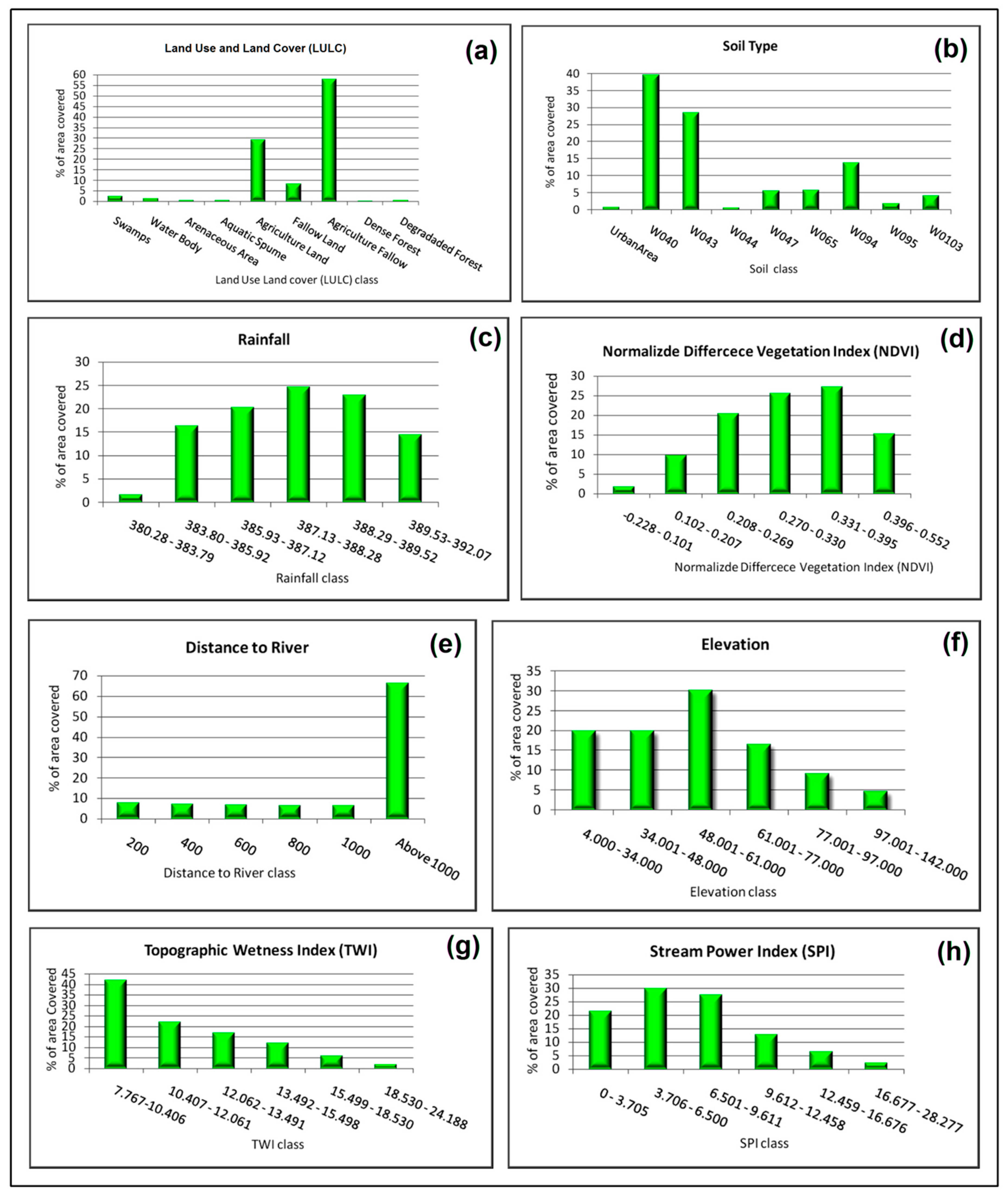
2.4.1. Land Use Land Cover (LULC)

The LULC of an area is largely influenced by surface runoff, infiltration rate, and evapotranspiration [47], and all of these factors directly or indirectly lead to flood occurrences. It is also known fact that there is a negative correlation between the high vegetation densities and frequency of flood occurrences [42]. In the present study, the LULC map was prepared using a Sentinel 2A satellite image, collected from the European Space Agency (ESA). The present LULC map was classified into eight classes, i.e., swamps, water body, arenaceous areas, aquatic spume, agricultural land, fallow land, agricultural fallow, dense forest, and degraded forest (Figure 4a). Among the eight LULC classes, agricultural fallow and agricultural land covered the most (87%) areas (Figure 5a).

2.4.2. Soil types

Soil is one of the important factors for occurrences of flood [48]. The pattern of the surface runoff, infiltration rate, and associated inundation largely depends on soil texture [43]. Furthermore, soil composition determines the water storage capacity, pattern of drainage channel, and permeability of water which mainly causes inundation [25]. The soil map (Figure 4b) in this area was prepared from the National Bureau of Soil Survey and Land Use planning (NBSSLUP) soil report. Table 2 shows the details about several soil types found in this study area. W040 soil type occupies the maximum area (40%), followed by W043 (28%) and W094 (14%) (Figure 5b).

2.4.3. Rainfall

Rainfall is the most relevant factor for occurrences of flood [49]. The magnitude of flood is largely dependent on the duration and intensity of rainfall. In this study, mean peak months of rainfall data were collected from the India Meteorological Department and India water portal website during the time from1984 to 2018. Subtropical monsoon-dominated eastern India received maximum rainfall during the months of June to September, i.e., peak monsoon months. The reason behind the selection of peak monsoon months is due to the presence of monsoon-dominated climatic characteristics. The time period (may be in a specific month or combination of few months) of maximum rainfall received in a monsoon-dominated climatic area are not the same every year, it varies from year to year. Thus, here we selected rainfall data for the time period of June to September, as eastern India received maximum rainfall during these peak months. The spatial distribution of rainfall map was prepared by using the inverse distance weighted (IDW) tool in the ArcGIS 10.4 platform. The Koiya river basin rainfall map was classified into six categories (Figure 4c). The rainfall map shows that middle of the northern part and the portion of lower areas received <385.92 mm rainfall and the part of western, southern, and south-eastern zones received >389.52 mm rainfall, in which the class of 387.13 to 388.28 was the maximum percentage (58.46%), followed by 388.29 to 389.52 and 385.93 to 387.12 (Figure 5c).

2.4.4. Normalized Difference Vegetation Index (NDVI)

The intensity of flood depends on vegetation cover and basically dense vegetation minimized the flood occurrences. Therefore, for estimation of vegetation characteristics, NDVI is widely used as a vegetation indices tool [50]. The NDVI value ranges from 0 to 1, in which 0, 0.2 to 0.4, and >0.5 represent barren or water land, grass land, and forest cover land, respectively [51]. In this study, the NDVI map was prepared through Landsat 8 OLI satellite image using Equation (1). The remote sensing-based satellite data were collected during the cloud-free month, i.e., November, after the rainy season (July to September) when vegetation is in the status of maximum greenery. The NDVI map was classified into six types (Figure 4d) and the class of 0.331 to 0.395 occupied maximum (27.32%) area, followed by the classes of 0.270 to 0.330 and 0.208 to 0.269 (Figure 5d). The map shows that the NDVI value in the upper course of the river basin area is very low, i.e., <0.207, and middle and lower courses of the basin area are covered by agricultural land, grass land, and forest areas, as NDVI value is significantly higher in this area.
NDVI = ( NIR R ) ( NIR + R )
where NIR and R is the spectral reflectance of near infrared and red band, respectively.

2.4.5. Distance to River

The assessment of FS is significantly dependent on the distance to river factor [52]. It is a fact that the area close to the river is more prone to flood and the area far away from the river is less prone to flood [53]. In this study, the distance to river map was prepared by using Euclidean distance tool in ArcGIS 10.4 platform. The distance to river map (Figure 4e) was classified into six categories and the class of above 1000 m occupied the maximum (68.21%) area in this study (Figure 5e).

2.4.6. Elevation

Elevation is considered as one of the noteworthy factors for flood occurrences and has been used in many research works [54]. Elevation basically controls the natural flow of water [55]. It is well known that a high elevated area is less vulnerable to flood and a low elevation area is highly affected by flood [35,56]. The elevation map in this study area was prepared using shuttle radar topographic mission (SRTM) of digital elevation model (DEM) of 30 m spatial resolution in GIS platform. The elevation map was also classified into six types (Figure 4f) and maximum (31%) area was covered by the class of 48 to 61m, i.e., the middle course of river basin area (Figure 5f). The elevation in the upper course area ranges between 61 m and142 m and in the lower course area elevation ranges from 4 m to 34 m. Thus, the lower course of river basin area is highly susceptible to occurrences of flooding.

2.4.7. Topographic Wetness Index (TWI)

The accumulation of flow water in terms of its spreading and depletion of surface water is represented through the TWI [45,57]. The saturation level of topography is indicated by TWI. A high value of TWI indicates the land is well saturated and prone to flood susceptibility and vice-versa [42]. The TWI map in this study area was prepared using Equation (2) and classified into six types (Figure 4g). The class of 7.767 to 10.406 covered the maximum (43.24%) area (Figure 5g). The TWI map shows that throughout the study area, the value of TWI is very low, i.e., < 12.061. In the middle and lower portions of basin area, there are some isolated places where TWI value is significantly higher, i.e., 15.499 to 24.188. Thus, these areas are saturated and influenced by flooding activity.
TWI = log e ( A s tan β )
where, A s is the catchment area in m2 and β is the gradient of the slope in radians.

2.4.8. Stream Power Index (SPI)

The water-induced surface runoff and associated erosional power are represented through SPI [7]. Higher and lower values of SPI indicate high and low erosional power, respectively, and the associated inundation phenomenon. The SPI map was prepared using Equation (3). The SPI map was also classified into six classes (Figure 4h) and the highest area (30.07%) is covered by the class of 3.706 to 6.500 (Figure 5h). The SPI map shows that the upper course of the basin, some isolated patches of southern portion, along with two sides of the middle river courses are more prone to erosional activities as the SPI value in these areas are significantly high (12.459 to 28.277). On the other side, the lower portion of basin area is dominated by low SPI value and indicates low erosional activities. Thus, due to erosional activities in the higher area of the upper course, sediment has been carried towards the down slope area, i.e., lower course, reduced the water holding capacity of river channel, and caused occurrences of flooding.
SPI = As tan β

2.5. Multicollinearity (MC) Test

The multi-collinearity (MC) test is the linear relationship among the several variables and it is a popular statistical method [58]. The MC problem occurs when several independent variables are correlated among each other in a regression model [59]. The MC test was carried out among the chosen FSCFs to reduce the possible error in the FS modelling. In this study, we used tolerance (TOL) and variance inflation factor (VIF) techniques for assessment of the MC test. If the threshold value of VIF is > 5 and TOL is < 0.1, thenthere is a MC problem in a dataset [60]. The following Equations of (4) and (5) were used to calculate the TOL and VIF value, respectively.
TOL = 1 R j 2
VIF = 1 TOL
where R j 2 indicates the coefficient of determination.

2.6. Relative Importance of Factors and Respective Sub-Class Factors

Several appropriate factors were used for FS assessment but not all the factors are equally responsible for the occurrences of flood. Therefore, identifying the relative importance of factors and their respective sub-class is indeed necessary for perfect evaluation of FS assessment. In this study, we used the random forest (RF) algorithm and the step-wise weight assessment ratio analysis (SWARA) method for identification of relative importance factors and sub-class factors, respectively.

2.6.1. Random Forest (RF)

RF is a popular ML algorithm which is based on the ensemble of binary decision tree, proposed by Breiman [61]. The bagging approach has been used to form a decision tree in the RF algorithm during the training phase [62]. The application of RF usually occurs in the case of classification, regression, and unsupervised learning. The advantage of the RF algorithm is that it has the ability to reduce generalization error more than any other ML model. Here, we applied the mean decrease accuracy (MDA) index within the RF model for identification of variables’ importance because traditional statistical methods are not capable of handling large data sizes. The following equation was used to calculate the value of variables’ importance through the MDA index [63].
VI j = 1 ntree t = 1 ntree EP tj E tj
where VI represents the relative importance of variables, E tj indicates the out-of-bag (OOB) error on tree t before permuting the values of X j , and EP tj indicates the OOB error on tree t after permuting the values of X j .

2.6.2. Step-Wise Weight Assessment Ratio Analysis (SWARA)

In this study, the importance of sub-class of respective variables was measured through SWARA weight, which was developed by [64]. It is one of the best decision analysis techniques and followed by stepwise weight assessment procedure. Expert opinion is essential for determining weightage in respective fields. Thus, the rank was given based on the expert’s knowledge, experience, and proper understanding [65]. The highest and lowest rank are occupied by most important and lowest criterion, respectively [66]. The SWARA method was computed using the following equations [67,68].
k j = { 1 j = 1 s j + 1 j > 1
where k j is the coefficient.
w j = { 1 j = 1 x j 1 k j j > 1
where w j is the recalculated weight. Finally, the relative weight of criteria was calculated by the following equation.
q j = w j k = 1 n w j

2.7. Machine Learning Methods for Flood Susceptibility Modelling

2.7.1. Hyperpipes (HP)

The algorithm of HP has the ability to perform the classification process in shortest time period with a huge number of variables [69]. The classification process in this algorithm is done based on the simple counts. In a broader way, the HP algorithm has been used in medical science [69], although literature studies also show that this algorithm has been used in various natural hazards susceptibility assessment like landslide [70]. It is a straightforward algorithm that builds a hyperpipe for each class in a given dataset. The function of the HP algorithm was run as follows [71]:
  • By using the training dataset, a single pipe was developed for each class and this pipe was matching with the respective class.
  • All the data were analyzed instance by instance.
  • If attribute value had not occurred yet, each instance value was attached to the respective pipe.
  • Comparison of instance value and attribute value was done through class pipes.
  • Finally, the instances were selected with the respective class pipe for optimal match.
The class of sample counts that has the maximum diverse values can be attributed to a specific class in the full training dataset [70]. For example, the training dataset contains classes in a set and finds each value at least once, therefore every instance tested value accurately fits into that pipe and ultimately is classified by that respective pipe’s class [72]. High recall rate can be found with this type of testing dataset in HP algorithm. Thus, various classes will be accurately recognized and the false alarm rate will also be equally identified as instances may also be falsely classified. Moreover, this algorithm is exceptionally fast with minimum memory footprints and especially simple. The illustration of HP can be explained as: in the dataset, all pipes are present as pipe1, pipe2, pipe3, and pipe4; and in that instance the number of matches are represent as 7, 0, 7, and 4, respectively; then the class of pipe3 is assigned as instance value [72].

2.7.2. Support Vector Regression (SVR)

The SVR model was proposed by Vapnik et al. [73] and it is a supervised ML algorithm. Basically, the SVR model was developed using the algorithm of support vector machine (SVM) classifiers [74]. The structure and control complex function was developed within a system through this algorithm. The advantage of SVR model is that it can maximize the nominal margin through regression task analysis [75]. Generally, the SVR model is applied when the training dataset is very complex, and this model solves this dataset through developing several curved margins [76]. The structural risk minimization (SRM) norm is an important parameter in the SVR model as it identifies the relationship between input and output variables [56]. Thus, SRM calculation is necessary in a SVR model and this can be calculated using Equations (10) and (11).
y = k ( z ) = v ( z ) + c
where the input data are represented through z = ( z 1 , z 2 , z n ) and the resultant value is shown by y b R l . In addition to this, v R l represents the weightage factor, c R l represents the constant number of the mathematical function, and l represents the data size in the respective model. ( z ) represents the irregular function to map the input dataset. To define v and c , the following equation can be used and was developed based on the SRM principles:
Minimize : [ 1 2 | | v | | 2 + P b = 1 1 ( ζ b + ζ b * ) ] Subjectto : { y b ( v ( z b ) + c b ) ε + ζ b ( v ( z b ) + c b ) y b ε + ζ b * ζ b , ζ b * 0
where P is the penalty factor which balances the model flatness and its risk, ζ b , ζ b * indicates loose variables, and ε represents the optimized performance of the model [77,78]. The following equation was used to solve the optimization problem through Lagrangian function:
L ( v , c , ζ b , ζ b * , β b , β b * , δ b , δ b * ) = 1 2 | | | v | 2 + P b = 1 l ( ζ b + ζ b * b = 1 l β b ( ζ b + ε y b + v ( z b z ) + c ) b = 1 l β b * ( ζ b * + ε +   y b v ( z b z ) c ) b = 1 l ( δ b ζ b + ζ b * δ b * )
in which the Lagrangian multipliers are represented by δ b ,   δ b * , β b   and   β b *
Subsequently, SVR can be calculated by:
K ( z ) = b = 1 l ( β b β b * ) m ( z , z b ) + c
where the kernel function expressed through m ( z , z b ) = ϕ ( z ) ,   ϕ ( zb ) .

2.7.3. Ensemble of HP-SVR

The ensemble approach may be defined as the combination of several single methods of statistical or ML algorithms. This ensemble model gives better overall prediction performance of the model’s output result. The ensemble model always gives a more optimal result than any single stand-alone ML model. Thus, several research studies have shown that various ensemble methods have been used in different natural hazards susceptibility assessment like slope stability [79], landslide [80], flood susceptibility assessment [6], and more. Therefore, in this study, we also used a novel ensemble of the HP and SVR models to get utmost prediction accuracy in the outcome result. The ensemble of these two single models was carried out in the statistical programming package R.

2.8. Accuracy Assessment

Validation and accuracy assessment is an important task for any kind of susceptibility modeling. Without validation, the output result does not have any implication in reality. Therefore, in this study we also used five popular statistical methods, namely sensitivity, specificity, accuracy, ROC-AUC, and Kappa coefficient analysis. In this study, accuracy assessment was used to assess the number of pixels in flood and non-flood areas. The following four indices were used for measuring accuracy, true positive (TP), true negative (TN), false positive (FP), and false negative (FN) [44]. ROC-AUC analysis is the most important tool for validation of a model and has been widely used among research groups. The graphical representation of ROC curve is expressed through X and Y axis and is represented as sensitivity (TP) and 1-specificity (FP), respectively. The value of AUC ranges from 0 (poor performance) to 1 (good performance) [81]. On the other hand, Kappa coefficient index method has also been used here to validate the respective models. The value of Kappa coefficient ranges from −1 (unreliable) to +1 (reliable) [82]. The following equations have been used to calculate the several statistical methods used in the validation purposes for this study.
Sensitivity = TP TP + FN
Specificity = TN FP + TN
Accuracy = TP + TN TP + TN + FP + FN
AUC = ( TP + TN ) ( P + N )
Kappa = P a P exp 1 P exp
P a = TP + TN TP + TN + FN + FP
P exp = ( TP + FN ) ( TP + FP ) + ( FP + TN ) ( FN + TN ) ( TP + TN + FN + FP )

3. Results

3.1. Multi-Collinearity (MC) Analysis

It is a well-known fact that the MC test is indeed necessary for improving the accuracy assessment by removing the bias among the variables for any kind of susceptibility modeling. Thus, in this research study, the MC test was carried out among the several variables to select suitable factors for FS modeling. The MC test was estimated through TOL and VIF techniques and eight appropriate parameters were selected for FS modelling. The result of TOL and VIF in the present research study ranged from 0.493 to 0.969 and 1.032 to 2.029, respectively, which has shown that the MC result is within the permissible threshold and free from MC problems. The lowest and highest TOL value were found in soil (0.493) and distance to river (0.969). Similarly, highest and lowest VIF value were found in soil (2.029) and distance to river (1.032) FS conditioning factors. The result of the MC test in all the variables is shown in Table 3.

3.2. Relative Importance of the Variables and Their Sub-Classes

Based on the literature studies and local geo-environmental factors, eight flood conditioning factors were selected and their MC test was carried out for FS modeling. It is also important to know which variables and their respective sub-classes are more important for occurrences of flood. Therefore, to know that, here we applied the method of mean decrease accuracy (MDA) of the RF algorithm and SWARA weight for relative importance of factors and their sub-classes respectively. Table 4 shows the result of relative importance of several factors identified through MDA methods. Thus, the output result shows that distance to river (0.91) is the most important factor for occurrences of flood followed by rainfall (0.84), LULC (0.66), SPI (0.54), soil (0.43), TWI (0.36), NDVI (0.28), and elevation (0.18). Therefore, the above factors are very much responsible for the occurrences of flood in this study area.
In the previous paragraph, we described the relative importance of several factors, but it is also necessary to know the importance of each sub-class of several respective factors on flood occurrences. Therefore, here we analyzed the weightage of each factor’s sub-classes by using the SWARA method, and the result is shown in Table 5. The result of the SWARA method shows that aquatic spume with weightage of 0.45 is most responsible for flood followed by agricultural land (0.16) and fallow land (0.12) in the LULC factors. On the other hand, arenaceous area, dense forest, and degraded forest with nil value of SWARA weightage are much less responsible for flood. In the case of soil type, W044 (0.37), W047 (0.25), and W065 (0.19) are associated with flood. Rainfall is one of the most significant parameters for occurrences of flood and the sub-classes of 380.28 to 383.79 (0.52), 388.29 to 389.52 (0.17), and 387.13 to 388.28 (0.11) are highly associated with flood occurrences. NDVI value ranges from −0.329 to −0.552, and the class of 0.395 to 0.552 is associated with high value of 0.23 followed by 0.331 to 0.395 (0.21) and 0.270 to 0.330 (0.17), and very low value consist of < −0.329 (0.11). In distance to river, the sub-class of < 400 m is highly responsible for flood occurrences as the SWARA weight of < 200 m and 200 to 400 m is 0.23 and 0.32, respectively. The area of low flood occurrences zone in distance to river are 1000 m and above 1000 m, as their respective values are 0.09 and 0.04. Elevation is one dominant factor for occurrences of flood. The sub-class of 4 to 34 m is most responsible for occurrences of flood with weightage value of 0.52 followed by 34 to 48 m (0.23) and 48 to 61 m (0.12). The very low zones for flood occurrences area are97 to 142 m, 61 to 77 m, and 77 to 97 m with weightage value is 0.02, 0.03, and 0.08 respectively. The sub-class of 10.407 to 12.061 of TWI (0.19) and in SPI, the sub-class of 9.612 to 12.458 (0.23) is highly associated with frequent flood occurrences in this study area.

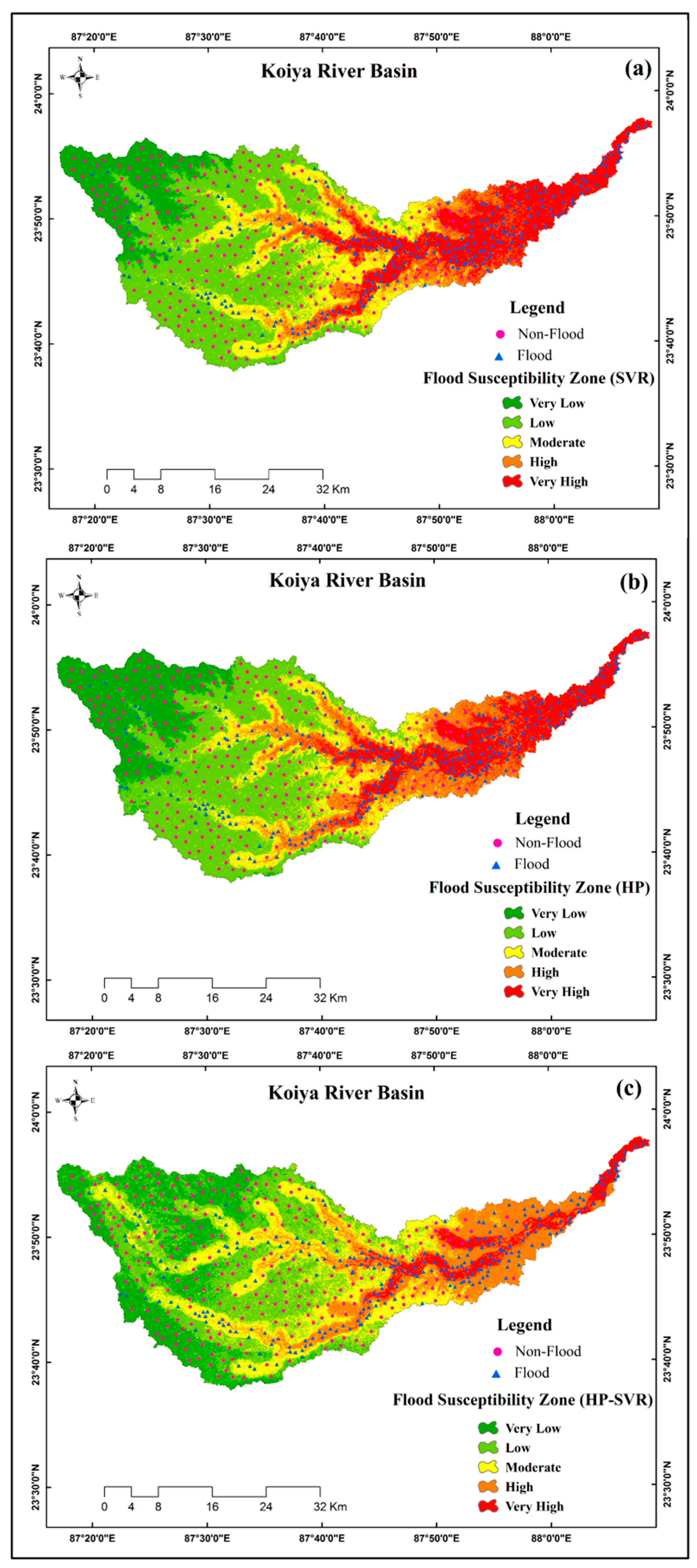
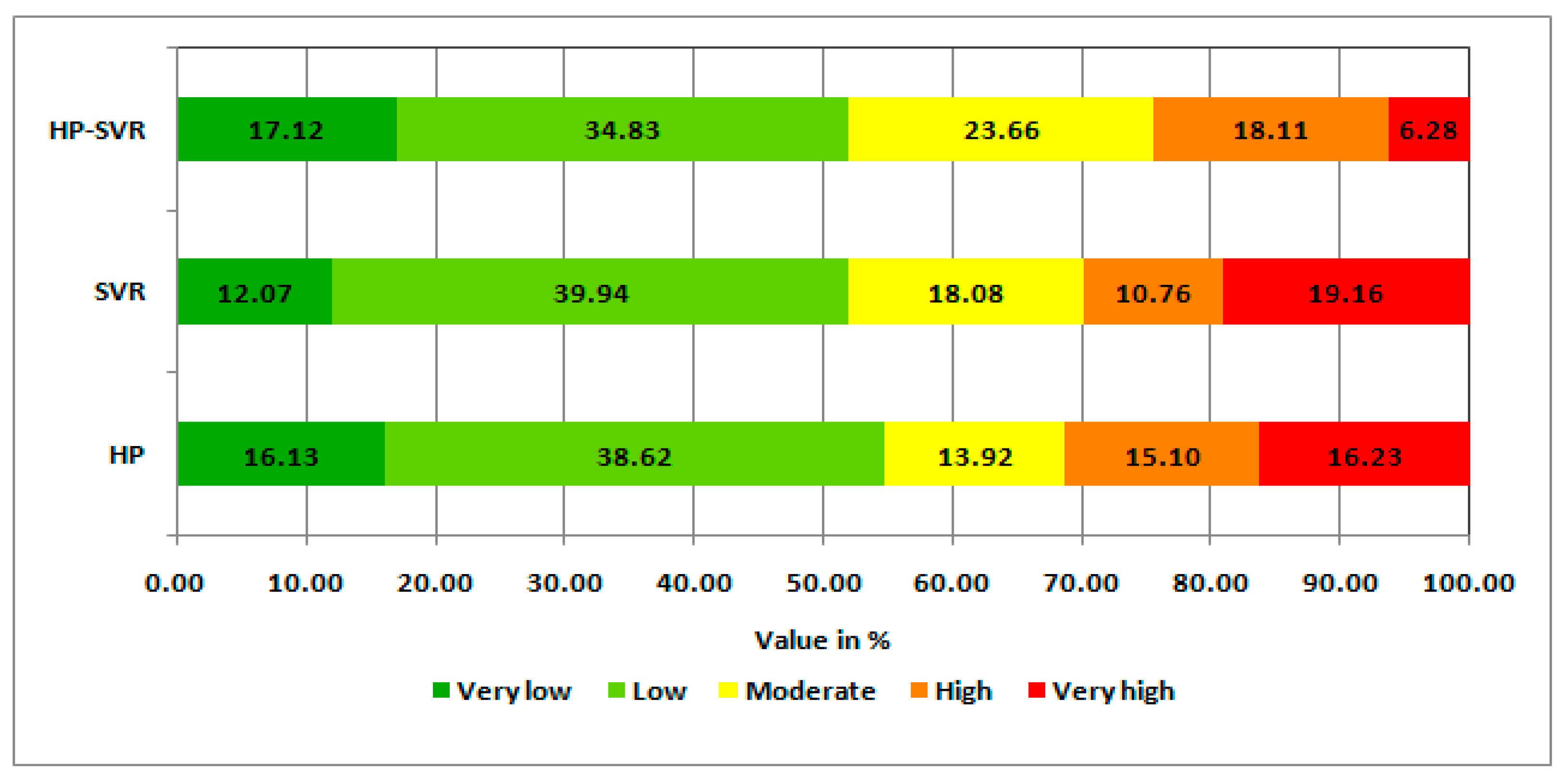
3.3. Spatial Assessment of Flood Susceptibility Mapping

The present research work of FS assessment was carried out using two ML algorithms of SVR and HP and one ensemble approach of SVR-HP in the Koiya river basin of Bengal Basin. The aforementioned model’s output maps are presented in Figure 6. In the purpose of better understanding the spatial distribution and their variation, all of these model’s output maps were classified into five categories by using Jenk’s natural breaks methods in the ArcGIS 10.4 platform. These classifications are very low, low, moderate, high, and very high, and have been symbolized with the same color for every zone in the respective maps prepared through ML algorithms. All of these maps have shown near regularity among the several susceptibility zones prepared for FS mapping. The FS map prepared through the SVR model is presented in Figure 6a and respective aerial coverage of five zones, i.e., very low, low, moderate, high, and very high are173.01 (12.07%), 572.55 (39.94%), 259.22 (18.08%), 154.23 (10.76%), and 274.69 (19.16%) km2 respectively (Figure 7). In the case of the HP model, the prepared FS map is shown in Figure 6b and aerial coverage by five zones, i.e., very low is 231.29 (16.13%), low is 553.69 (38.62%), moderate is 199.50 (13.92%), high is 216.51 (15.10%), and very high is 232.70 (16.23%) km2 (Figure 7). The ensemble of SVR-HP approach’s produced map is presented in Figure 6c and the aerial coverage and respective percentage of five zones, i.e., very low, low, moderate, high, and very high are 245.50 (17.12%), 499.31 (34.83%), 339.19 (23.66%), 259.61 (18.11%), and 90.09 (6.28%) sq. km, respectively (Figure 7). Among the three methods, ensemble of HP-SVR mapping shows the greatest area (245.50 km2) of very low FS zones followed by HP (231.29 sq.km) and SVR (173.01 km2). On the other side, the largest area of very high FS zone is covered by the SVR-produced map (274.69 km2) followed by HP (232.70 km2) and HP-SVR (90.09 km2). As a general rule, very high flood prone areas are found in the lower courses of the present river basin area and very low flood prone areas are found in the upper courses of the river, as was found in this research study.

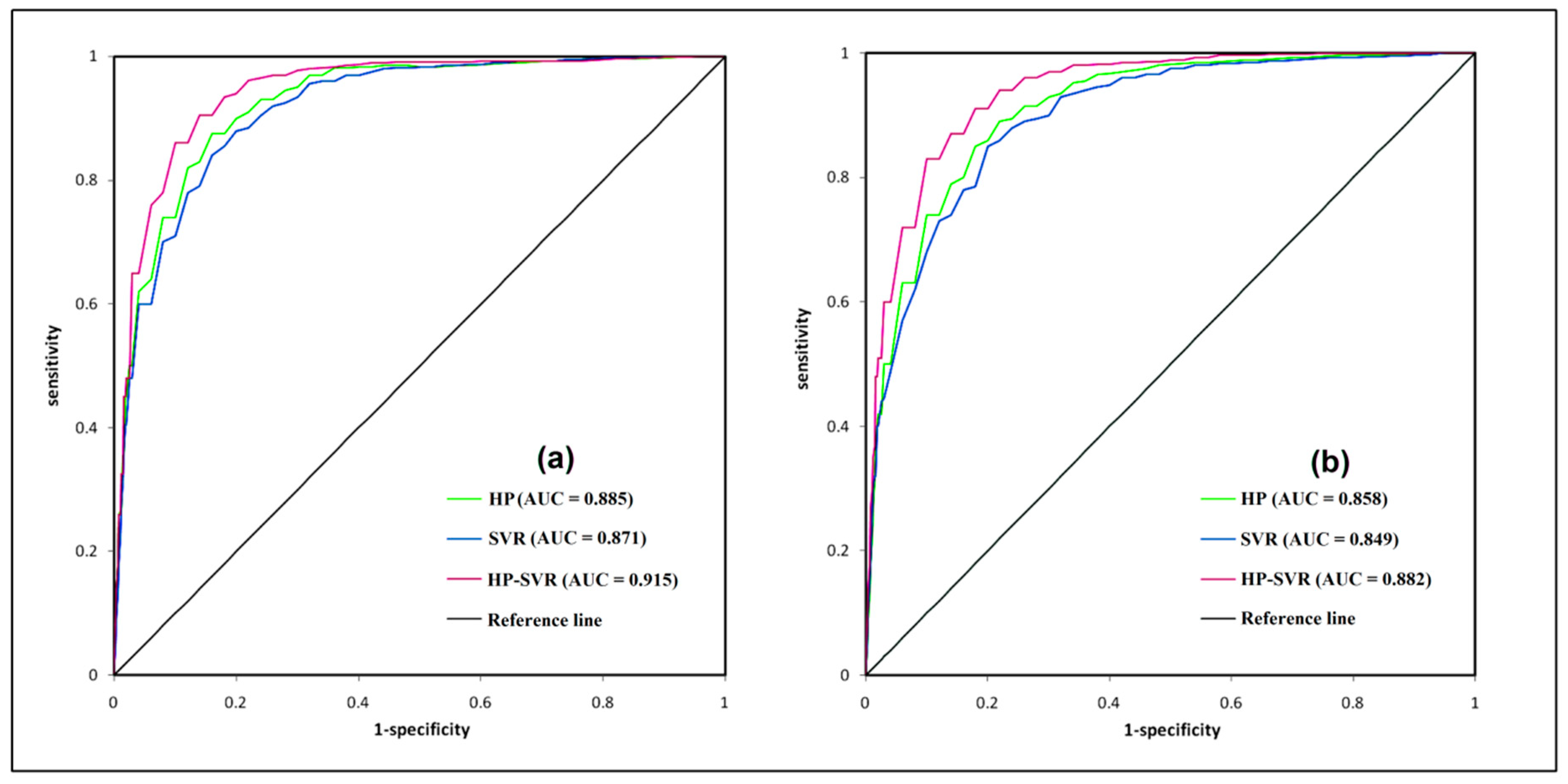
3.4. Evaluation of Validation Performance

The validation and accuracy assessment of predictive performance is indeed necessary for optimal analysis of the respective model’s result. In this study, evaluation of validation performance was carried out using the most popular five statistical methods namely sensitivity, specificity, accuracy, AUC, and Kappa coefficient analysis. The aforementioned statistical methods were quantitatively analyzed and were the most consistent for validation and accuracy assessment of respective model’s result. Accuracy is determining the quality of the information derived from several sources, generally remote sensed data. Thus, in the purpose of modeling and mapping of susceptibility analysis, where remote sensed data were used for management and decision-making, accuracy measurement is very much important. The success and prediction result of all the models was carried out by using training (flood points) and testing (non-flood points) dataset. The AUC tool is one of most important tools used for validation performance through measuring the diagnostic capability of the model. The graphical construction of the AUC analysis for the training and testing dataset of aforementioned three ML models is presented in Figure 8a,b respectively. In addition, the quantitative results of the aforementioned five statistical indices are presented in Figure 9. The AUC value for the HP-SVR, HP, and SVR models in the training dataset is 0.915, 0.885, and 0.871 (Figure 8a) and in the testing dataset is 0.882, 0.858, and 0.849 (Figure 8b), respectively. In the case of sensitivity, the values of HP-SVR, HP, and SVR models in the training and testing dataset are0.932, 0.922, and 0.897 (Figure 8a), and 0.918, 0.880, and 0.875 (Figure 8b) respectively. For specificity, the values of HP-SVR, HP, and SVR model in the training and testing dataset are0.902, 0.890, and 0.871 (Figure 9a) and 0.857, 0.864, and 0.846 (Figure 9b), respectively. In accuracy, HP-SVR, HP, and SVR models consist of 0.918, 0.908, and 0.886 (Figure 9a) for training and 0.886, 0.873, and 0.860 (Figure 9b) for testing dataset, respectively. In the case of Kappa coefficient, HP-SVR, HP, and SVR model consist of 0.835, 0.813, and 0.767(Figure 9a) and 0.772, 0.745, and 0.721 (Figure 9b) for training and testing dataset respectively. From the above discussion, it is stated that the ensemble model of HP-SVR is the most optimal model for assessment of FS spatial prediction analysis, as it is occupied with the highest value in aforementioned five validation methods, followed by HP and SVR.

4. Discussion

In the last decade, machine learning and fuzzy models have received considerable attention [83,84,85,86,87], because these methods are so applicable to modeling of spatial data [88,89,90,91,92]. The FSCFs’ value evaluation is crucial for planners and policy makers, with a small allocation of resources, for better usage of resources, and optimum productivity. An estimation of the value of spatial FSCF modeling is carried out means of bivariate models when their weighting assignment is evaluated by means of frequency ratio (FR), weights-of-evidence (WOE), logistic regression (LR), analytic hierarchy process (AHP), etc. However, before using models for spatial modeling and mapping, all FSCFs would be given a pre-analyzed weighting or significance assignment [2,53]. A variety of experiments are available in which the relative significance of variables was determined using various techniques before spatial modeling. Different strategies have been evaluated on the same set of FSCFs to pick the best from the collection, but the validity of FSCFs is influenced and identified by the kind of topography and data used to extract such FSCFs. Therefore, due to different variables involved in planning FSCF, the efficiency of models is impaired. Based on the topographical, hydro-climatic, and multi-collinearity analysis we selected eight appropriate FSCFs for this study area. The selection of a system for determining relative significance was therefore not rigid or confined to any particular model. The random forest model was used for determining the relative value of each conditioning factor in the current work, along with SWARA weight method which was also used to identify importance of factor’s sub-classes on FS assessment. The results show that the distance to river, rainfall, NDVI, and LULC are of the utmost importance compared to the other factors. As rivers provide the key source of fluvial floods, especially on plains such as the Koiya River mouth, this frequently causes havoc [42]. The intensity of heavy and long rainfall causes a high rate of surface runoff in a downward direction, i.e., towards river channel. Thus, this phenomenon is responsible for increasing the stream’s water level and reducing the water holding capacity within the stream channel courses. As a result, associated overflow of water starts from the stream channel and inundation occurs to the nearby surrounding areas due to the present of low-lying area. At the same time, rainfall and LULC are also found as significant predictive factors for flooding due to the nearly flat surface topography in the region analyzed and higher rainfall [42]. LULC and NDVI also play a significant role for FS as vegetation density reduces surface runoff, percolates water to sub-surface areas through tree roots, and minimizes the incidence of flood occurrences. On the other side, other variables i.e., soil, elevation, TWI and SPI have also impacted on FS analysis. The characteristics of soil texture determined the surface flow and erosional activity, which is responsible for reducing the river depth and associated flooding condition. TWI and SPI determined the spatial spreading of surface runoff [45]. In a case study on FS analysis in Koiya river, both statistical, i.e., evidential belief function (EBF) and logistic regression (LR), and ensemble of EBF-LR models performed very well, with their AUCROC system values being 0.890, 0.882, and 0.906 respectively, including additional dependent matrices, assessing their performance [42]. In the current study, we selected HP, SVR, and their ensemble of HP-SVR for modelling and mapping of FS. The validation result showed that AUC value ranges from 0.871 to 0.915 and 0.849 to 0.882 in training and validation elements for all models, respectively. The performance of the ensemble model is excellent, i.e., 0.915 (training) and 0.879 (testing), that is why we are proposing this model for flood susceptibility modeling. In a research study on landslide susceptibility analysis based on HP algorithms, it has been shown that ensemble of HP model with AdaBoost (0.933), Bagging (0.950), Dagging (0.937), and Real AdaBoost (0.968) gave much better performance in AUC analysis than a single HP model (0.895) [71]. Thus, keeping this in view, here, an ensemble of HP-SVR was applied in FS analysis to get better predictive performance. Various differences in both findings using the same models can emerge due to the different topographic structure and the choice of FSCFs [2,93]. The efficiency of the models used during training and validation in this analysis has improved considerably. In the light of projections of global climate change, the use of such advanced tools with high precision to forecast areas potentially impacted by floods is highly important. In the future, however, there will be a rise in the occurrence of inundations owing to changes in rainfall manifestations and the rain will be more torrential [9]. It should be noted that, due to deforestation practices carried out in large areas in the plain region of the Indian Bengal Basin and also due to the expansion of built-up areas causing further conversion to impenetrable areas, the severity of floods will increase in the future [94]. The practices of deforestation and rising intensity and frequency of flooding would have a significant consequence on the potential bed load transport as well. In the event of a flood, sediment transport may be particularly hazardous to the properties and infrastructure components affected by the event. It is therefore of considerable importance that the torrential catchments vulnerable to sediment transport around the Koiya basin should be established in future research work.

5. Conclusions

As one of the worst flood-affected regions in India, the eastern fringe of the Bengal basins still aging behind proper policies designed to deal with the damages incurred by the threat. The aim should be to reduce the losses in relation to environmental sustainability hydraulic ventures, the development of areas to be used for identification and settlement areas, updates, precision and verifiable areas subject to flood, their vulnerability, etc., in order to conduct the successful decision-making process in the region that is critically affected by the flood occurrence. In the present study, both machine training models, SVR and HP, and their ensemble performed very well, and the AUCROC system, including additional dependent matrices, assessed their performance. The AUC value in the training and validation stages ranged from 0.871 to 0.915 and 0.849 to 0.882, respectively for all the models. The performance of the ensemble model was excellent, i.e., 0.915, which is why we are proposing this model for flood susceptibility modeling. The findings of this analysis can be used effectively by the National Disaster Management Authority, India to improve the precision of flood prediction and warning. The findings of this study can be a valuable guide for central and local authorities in terms of strategic implications, which should give priority to flood-related areas.

Author Contributions

Conceptualization, A.S., S.C.P., and A.A. (Alireza Arabameri); data curation, A.S., S.C.P., and A.A. (Alireza Arabameri); methodology, A.S., S.C.P., and A.A. (Alireza Alabameri); writing—original draft A.S., S.C.P., I.C., R.C. (Rabin Chakrabortty), and A.A. (Alireza Arabameri); writing—review and editing, A.S., S.C.P., I.C., R.C. (Rabin Chakrabortty), T.B., R.C. (Romulus Costache), A.A. (Alireza Arabameri), S.P., and A.A. (Aman Arora). All authors have read and agreed to the published version of the manuscript.

Funding

This research was partly funded by the Austrian Science Fund (FWF) through the Doctoral College GIScience (DK W 1237-N23) at the University of Salzburg.

Institutional Review Board Statement

Not applicable.

Informed Consent Statement

Not applicable.

Data Availability Statement

All flooding data, shapefile and code will be made available on request to the correspondent author’s email with appropriate justification.

Acknowledgments

Open Access Funding by the Austrian Science Fund (FWF).

Conflicts of Interest

The authors declare no conflict of interest.

References

  1. Mosavi, A.; Golshan, M.; Janizadeh, S.; Choubin, B.; Melesse, A.M.; Dineva, A.A. Ensemble Models of GLM, FDA, MARS, and RF for Flood and Erosion Susceptibility Mapping: A Priority Assessment of Sub-Basins. Geocarto Int. 2020, 1–20. [Google Scholar] [CrossRef]
  2. Arora, A.; Arabameri, A.; Pandey, M.; Siddiqui, M.A.; Shukla, U.K.; Bui, D.T.; Mishra, V.N.; Bhardwaj, A. Optimization of State-of-the-Art Fuzzy-Metaheuristic ANFIS-Based Machine Learning Models for Flood Susceptibility Prediction Mapping in the Middle Ganga Plain, India. Sci. Total. Environ. 2021, 750, 141565. [Google Scholar] [CrossRef] [PubMed]
  3. Keesstra, S.; Mol, G.; De Leeuw, J.; Okx, J.; Molenaar, C.; De Cleen, M.; Visser, S. Soil-Related Sustainable Development Goals: Four Concepts to Make Land Degradation Neutrality and Restoration Work. Land 2018, 7, 133. [Google Scholar] [CrossRef] [Green Version]
  4. Shirzadi, A.; Soliamani, K.; Habibnejhad, M.; Kavian, A.; Chapi, K.; Shahabi, H.; Chen, W.; Khosravi, K.; Thai Pham, B.; Pradhan, B.; et al. Novel GIS Based Machine Learning Algorithms for Shallow Landslide Susceptibility Mapping. Sensors 2018, 18, 3777. [Google Scholar] [CrossRef] [PubMed]
  5. Kalantari, Z.; Ferreira, C.S.S.; Koutsouris, A.J.; Ahlmer, A.-K.; Cerdà, A.; Destouni, G. Assessing Flood Probability for Transportation Infrastructure Based on Catchment Characteristics, Sediment Connectivity and Remotely Sensed Soil Moisture. Sci. Total Environ. 2019, 661, 393–406. [Google Scholar] [CrossRef]
  6. Band, S.S.; Janizadeh, S.; Chandra Pal, S.; Saha, A.; Chakrabortty, R.; Melesse, A.M.; Mosavi, A. Flash Flood Susceptibility Modeling Using New Approaches of Hybrid and Ensemble Tree-Based Machine Learning Algorithms. Remote Sens. 2020, 12, 3568. [Google Scholar] [CrossRef]
  7. Wang, Y.; Hong, H.; Chen, W.; Li, S.; Panahi, M.; Khosravi, K.; Shirzadi, A.; Shahabi, H.; Panahi, S.; Costache, R. Flood Susceptibility Mapping in Dingnan County (China) Using Adaptive Neuro-Fuzzy Inference System with Biogeography Based Optimization and Imperialistic Competitive Algorithm. J. Environ. Manag. 2019, 247, 712–729. [Google Scholar] [CrossRef]
  8. Ligtvoet, W.; Witte, F.; Goldschmidt, T.; Oijen, M.J.P.V.; Wanink, J.H.; Goudswaard, P.C. Species Extinction and Concomitant Ecological Changes in Lake Victoria. Neth. J. Zool. 1991, 42, 214–232. [Google Scholar] [CrossRef] [Green Version]
  9. Roy, P.; Chandra Pal, S.; Chakrabortty, R.; Chowdhuri, I.; Malik, S.; Das, B. Threats of Climate and Land Use Change on Future Flood Susceptibility. J. Clean. Prod. 2020, 272, 122757. [Google Scholar] [CrossRef]
  10. Arabameri, A.; Saha, S.; Mukherjee, K.; Blaschke, T.; Chen, W.; Ngo, P.T.T.; Band, S.S. Modeling Spatial Flood Using Novel Ensemble Artificial Intelligence Approaches in Northern Iran. Remote Sens. 2020, 12, 3423. [Google Scholar] [CrossRef]
  11. Rozalis, S.; Morin, E.; Yair, Y.; Price, C. Flash Flood Prediction Using an Uncalibrated Hydrological Model and Radar Rainfall Data in a Mediterranean Watershed under Changing Hydrological Conditions. J. Hydrol. 2010, 394, 245–255. [Google Scholar] [CrossRef]
  12. Mirza, M.M.Q. Climate Change, Flooding in South Asia and Implications. Reg. Environ. Chang. 2011, 11, 95–107. [Google Scholar] [CrossRef]
  13. Bandyopadhyay, S.; Ghosh, P.K.; Jana, N.C.; Sinha, S. Probability of Flooding and Vulnerability Assessment in the Ajay River, Eastern India: Implications for Mitigation. Environ. Earth Sci. 2016, 75, 578. [Google Scholar] [CrossRef]
  14. Ganugula, G.; Venkata, B.; Sinha, R. GIS in Flood Hazard Mapping: A Case Study of Kosi River Basin, India. 2005. Available online: http://www.gisdevelopment.net/application/natural_hazards/floods/floods001pf.htm (accessed on 9 September 2020).
  15. Kale, V.S. Is Flooding in South Asia Getting Worse and More Frequent? Singap. J. Trop. Geogr. 2014, 35, 161–178. [Google Scholar] [CrossRef]
  16. Han, C.; Zhang, B.; Chen, H.; Wei, Z.; Liu, Y. Spatially distributed crop model based on remote sensing. Agric. Water Manag. 2019, 218, 165–173. [Google Scholar] [CrossRef]
  17. Zuo, C.; Chen, Q.; Tian, L.; Waller, L.; Asundi, A. Transport of intensity phase retrieval and computational imaging for partially coherent fields: The phase space perspective. Opt. Lasers Eng. 2015, 71, 20–32. [Google Scholar] [CrossRef]
  18. Yan, J.; Pu, W.; Zhou, S.; Liu, H.; Bao, Z. Collaborative Detection and Power Allocation Framework for Target Tracking in Multiple Radar System. Inf. Fusion 2019, 55, 173–183. [Google Scholar] [CrossRef]
  19. Zuo, C.; Chen, Q.; Gu, G.; Feng, S.; Feng, F.; Li, R.; Shen, G. High-speed three-dimensional shape measurement for dynamic scenes using bi-frequency tripolar pulse-width-modulation fringe projection. Opt. Lasers Eng. 2013, 51, 953–960. [Google Scholar] [CrossRef]
  20. Chao, L.; Zhang, K.; Li, Z.; Zhu, Y.; Wang, J.; Yu, Z. Geographically weighted regression based methods for merging satellite and gauge precipitation. J. Hydrol. 2018, 558, 275–289. [Google Scholar] [CrossRef]
  21. Zhu, J.; Wu, P.; Chen, M.; Kim, M.J.; Wang, X.; Fang, T. Automatically Processing IFC Clipping Representation for BIM and GIS Integration at the Process Level. Appl. Sci. 2020, 10, 2009. [Google Scholar] [CrossRef] [Green Version]
  22. Zhu, J.; Wang, X.; Wang, P.; Wu, Z.; Kim, M.J. Integration of BIM and GIS: Geometry from IFC to shapefile using open-source technology. Autom. Constr. 2019, 102, 105–119. [Google Scholar] [CrossRef]
  23. Zhu, J.; Wang, X.; Chen, M.; Wu, P.; Kim, M.J. Integration of BIM and GIS: IFC geometry transformation to shapefile using enhanced open-source approach. Autom. Constr. 2019, 106, 102859. [Google Scholar] [CrossRef]
  24. Wu, T.; Cao, J.; Xiong, L.; Zhang, H. New Stabilization Results for Semi-Markov Chaotic Systems with Fuzzy Sampled-Data Control. Complexity 2019. [Google Scholar] [CrossRef]
  25. Wu, T.; Xiong, L.; Cheng, J.; Xie, X. New results on stabilization analysis for fuzzy semi-Markov jump chaotic systems with state quantized sampled-data controller. Inf. Sci. 2020, 521, 231–250. [Google Scholar] [CrossRef]
  26. Shi, K.; Wang, J.; Tang, Y.; Zhong, S. Reliable asynchronous sampled-data filtering of T–S fuzzy uncertain delayed neural networks with stochastic switched topologies. Fuzzy Sets Syst. 2020, 381, 1–25. [Google Scholar] [CrossRef]
  27. Chen, H.; Qiao, H.; Xu, L.; Feng, Q.; Cai, K. A Fuzzy Optimization Strategy for the Implementation of RBF LSSVR Model in Vis–NIR Analysis of Pomelo Maturity. IEEE Trans. Ind. Inform. 2019, 15, 5971–5979. [Google Scholar] [CrossRef]
  28. Shi, K.; Wang, J.; Zhong, S.; Tang, Y.; Cheng, J. Non-fragile memory filtering of TS fuzzy delayed neural networks based on switched fuzzy sampled-data control. Fuzzy Sets Syst. 2020, 394, 40–64. [Google Scholar] [CrossRef]
  29. Xu, M.; Li, T.; Wang, Z.; Deng, X.; Yang, R.; Guan, Z. Reducing complexity of HEVC: A deep learning approach. IEEE Trans. Image Process. 2018, 27, 5044–5059. [Google Scholar] [CrossRef] [Green Version]
  30. Lv, Z.; Qiao, L. Deep belief network and linear perceptron based cognitive computing for collaborative robots. Appl. Soft Comput. 2020, 92, 106300. [Google Scholar] [CrossRef]
  31. Lv, Z.; Xiu, W. Interaction of edge-cloud computing based on SDN and NFV for next generation IoT. IEEE Internet Things J. 2019, 7, 5706–5712. [Google Scholar] [CrossRef]
  32. Chen, H.; Chen, A.; Xu, L.; Xie, H.; Qiao, H.; Lin, Q.; Cai, K. A deep learning CNN architecture applied in smart near-infrared analysis of water pollution for agricultural irrigation resources. Agric. Water Manag. 2020, 240, 106303. [Google Scholar] [CrossRef]
  33. Qian, J.; Feng, S.; Tao, T.; Hu, Y.; Li, Y.; Chen, Q.; Zuo, C. Deep-learning-enabled geometric constraints and phase unwrapping for single-shot absolute 3D shape measurement. APL Photonics 2020, 5, 046105. [Google Scholar] [CrossRef]
  34. Qian, J.; Feng, S.; Li, Y.; Tao, T.; Han, J.; Chen, Q.; Zuo, C. Single-shot absolute 3D shape measurement with deep-learning-based color fringe projection profilometry. Opt. Lett. 2020, 45, 1842–1845. [Google Scholar] [CrossRef] [PubMed]
  35. Liu, S.; Chan, F.T.S.; Ran, W. Decision making for the selection of cloud vendor: An improved approach under group decision-making with integrated weights and objective/subjective attributes. Expert Syst. Appl. 2016, 55, 37–47. [Google Scholar] [CrossRef]
  36. Wu, C.; Wu, P.; Wang, J.; Jiang, R.; Chen, M.; Wang, X. Critical review of data-driven decision-making in bridge operation and maintenance. Struct. Infrastruct. Eng. 2020, 1–24. [Google Scholar] [CrossRef]
  37. Arabameri, A.; Rezaei, K.; Cerdà, A.; Conoscenti, C.; Kalantari, Z. A Comparison of Statistical Methods and Multi-Criteria Decision Making to Map Flood Hazard Susceptibility in Northern Iran. Sci. Total Environ. 2019, 660, 443–458. [Google Scholar] [CrossRef]
  38. Lee, M.; Kang, J.; Jeon, S. Application of Frequency Ratio Model and Validation for Predictive Flooded Area Susceptibility Mapping Using GIS. In Proceedings of the 2012 IEEE International Geoscience and Remote Sensing Symposium, Munich, Germany, 22–27 July 2012; pp. 895–898. [Google Scholar]
  39. Rahmati, O.; Zeinivand, H.; Besharat, M. Flood Hazard Zoning in Yasooj Region, Iran, Using GIS and Multi-Criteria Decision Analysis. Geomat. Nat. Hazards Risk 2016, 7, 1000–1017. [Google Scholar] [CrossRef] [Green Version]
  40. Tehrany, M.S.; Pradhan, B.; Mansor, S.; Ahmad, N. Flood Susceptibility Assessment Using GIS-Based Support Vector Machine Model with Different Kernel Types. CATENA 2015, 125, 91–101. [Google Scholar] [CrossRef]
  41. Arabameri, A.; Saha, S.; Chen, W.; Roy, J.; Pradhan, B.; Bui, D.T. Flash Flood Susceptibility Modelling Using Functional Tree and Hybrid Ensemble Techniques. J. Hydrol. 2020, 587, 125007. [Google Scholar] [CrossRef]
  42. Chowdhuri, I.; Pal, S.C.; Chakrabortty, R. Flood Susceptibility Mapping by Ensemble Evidential Belief Function and Binomial Logistic Regression Model on River Basin of Eastern India. Adv. Space Res. 2020, 65, 1466–1489. [Google Scholar] [CrossRef]
  43. Zhang, K.; Wang, Q.; Chao, L.; Ye, J.; Li, Z.; Yu, Z.; Yang, T.; Ju, Q. Ground Observation-based Analysis of Soil Moisture Spatiotemporal Variability Across A Humid to Semi-Humid Transitional Zone in China. J. Hydrol. 2019, 574, 903–914. [Google Scholar] [CrossRef]
  44. Bellu, A.; Sanches Fernandes, L.F.; Cortes, R.M.V.; Pacheco, F.A.L. A Framework Model for the Dimensioning and Allocation of a Detention Basin System: The Case of a Flood-Prone Mountainous Watershed. J. Hydrol. 2016, 533, 567–580. [Google Scholar] [CrossRef]
  45. Samanta, R.K.; Bhunia, G.S.; Shit, P.K.; Pourghasemi, H.R. Flood Susceptibility Mapping Using Geospatial Frequency Ratio Technique: A Case Study of Subarnarekha River Basin, India. Model. Earth Syst. Environ. 2018, 4, 395–408. [Google Scholar] [CrossRef]
  46. Tehrany, M.S.; Shabani, F.; Jebur, M.N.; Hong, H.; Chen, W.; Xie, X. GIS-Based Spatial Prediction of Flood Prone Areas Using Standalone Frequency Ratio, Logistic Regression, Weight of Evidence and Their Ensemble Techniques. Geomat. Nat. Hazards Risk 2017, 8, 1538–1561. [Google Scholar] [CrossRef]
  47. Zhang, K.; Ruben, G.B.; Li, X.; Li, Z.; Yu, Z.; Xia, J.; Dong, Z. A comprehensive assessment framework for quantifying climatic and anthropogenic contributions to streamflow changes: A case study in a typical semi-arid North China basin. Environ. Model. Softw. 2020, 128, 104704. [Google Scholar] [CrossRef]
  48. Souissi, D.; Zouhri, L.; Hammami, S.; Msaddek, M.H.; Zghibi, A.; Dlala, M. GIS-Based MCDM—AHP Modeling for Flood Susceptibility Mapping of Arid Areas, Southeastern Tunisia. Geocarto Int. 2020, 35, 991–1017. [Google Scholar] [CrossRef]
  49. Dano, U.L.; Balogun, A.-L.; Matori, A.-N.; Wan Yusouf, K.; Abubakar, I.R.; Said Mohamed, M.A.; Aina, Y.A.; Pradhan, B. Flood Susceptibility Mapping Using GIS-Based Analytic Network Process: A Case Study of Perlis, Malaysia. Water 2019, 11, 615. [Google Scholar] [CrossRef] [Green Version]
  50. Pal, S.C.; Chakrabortty, R.; Malik, S.; Das, B. Application of Forest Canopy Density Model for Forest Cover Mapping Using LISS-IV Satellite Data: A Case Study of Sali Watershed, West Bengal. Model. Earth Syst. Environ. 2018, 4, 853–865. [Google Scholar] [CrossRef]
  51. Khosravi, K.; Pourghasemi, H.R.; Chapi, K.; Bahri, M. Flash Flood Susceptibility Analysis and Its Mapping Using Different Bivariate Models in Iran: A Comparison between Shannon’s Entropy, Statistical Index, and Weighting Factor Models. Environ. Monit. Assess 2016, 188, 656. [Google Scholar] [CrossRef]
  52. Choubin, B.; Moradi, E.; Golshan, M.; Adamowski, J.; Sajedi-Hosseini, F.; Mosavi, A. An Ensemble Prediction of Flood Susceptibility Using Multivariate Discriminant Analysis, Classification and Regression Trees, and Support Vector Machines. Sci. Total Environ. 2019, 651, 2087–2096. [Google Scholar] [CrossRef]
  53. Malik, S.; Chandra Pal, S.; Chowdhuri, I.; Chakrabortty, R.; Roy, P.; Das, B. Prediction of Highly Flood Prone Areas by GIS Based Heuristic and Statistical Model in a Monsoon Dominated Region of Bengal Basin. Remote Sens. Appl. Soc. Environ. 2020, 19, 100343. [Google Scholar] [CrossRef]
  54. Tiryaki, M.; Karaca, O. Flood Susceptibility Mapping Using GIS and Multicriteria Decision Analysis: Saricay-Çanakkale (Turkey). Arab. J. Geosci. 2018, 11, 364. [Google Scholar] [CrossRef]
  55. Xi, W.; Li, G.; Moayedi, H.; Nguyen, H. A particle-based optimization of artificial neural network for earthquake-induced landslide assessment in Ludian county, China. Geomat. Nat. Hazards Risk. 2019, 10, 1750–1771. [Google Scholar] [CrossRef] [Green Version]
  56. Das, B.; Pal, S.C.; Malik, S.; Chakrabortty, R. Living with Floods through Geospatial Approach: A Case Study of Arambag C.D. Block of Hugli District, West Bengal, India. SN Appl. Sci. 2019, 1, 329. [Google Scholar] [CrossRef] [Green Version]
  57. Bui, D.T.; Moayedi, H.; Kalantar, B.; Osouli, A.; Pradhan, B.; Nguyen, H.; Rashid, A.S.A. A Novel Swarm Intelligence—Harris Hawks Optimization for Spatial Assessment of Landslide Susceptibility. Sensors 2019, 19, 3590. [Google Scholar] [CrossRef] [Green Version]
  58. Alin, A. Multicollinearity. Wiley Interdiscip. Rev. Comput. Stat. 2010, 2, 370–374. [Google Scholar] [CrossRef]
  59. Arabameri, A.; Pradhan, B.; Rezaei, K.; Yamani, M.; Pourghasemi, H.R.; Lombardo, L. Spatial Modelling of Gully Erosion Using Evidential Belief Function, Logistic Regression, and a New Ensemble of Evidential Belief Function–Logistic Regression Algorithm. Land Degrad. Dev. 2018, 29, 4035–4049. [Google Scholar] [CrossRef]
  60. Khosravi, K.; Pham, B.T.; Chapi, K.; Shirzadi, A.; Shahabi, H.; Revhaug, I.; Prakash, I.; Tien Bui, D. A Comparative Assessment of Decision Trees Algorithms for Flash Flood Susceptibility Modeling at Haraz Watershed, Northern Iran. Sci. Total Environ. 2018, 627, 744–755. [Google Scholar] [CrossRef]
  61. Breiman, L. Random Forests. Mach. Learn. 2001, 45, 5–32. [Google Scholar] [CrossRef] [Green Version]
  62. Breiman, L. Bagging Predictors. Mach. Learn. 1996, 24, 123–140. [Google Scholar] [CrossRef] [Green Version]
  63. Han, H.; Guo, X.; Yu, H. Variable Selection Using Mean Decrease Accuracy and Mean Decrease Gini Based on Random Forest. In Proceedings of the 2016 7th IEEE International Conference on Software Engineering and Service Science (ICSESS), Beijing, China, 26–28 August 2016; pp. 219–224. [Google Scholar]
  64. Keršuliene, V.; Zavadskas, E.K.; Turskis, Z. Selection of Rational Dispute Resolution Method by Applying New Step-wise Weight Assessment Ratio Analysis (Swara). J. Bus. Econ. Manag. 2010, 11, 243–258. [Google Scholar] [CrossRef]
  65. Chowdhuri, I.; Pal, S.C.; Arabameri, A.; Saha, A.; Chakrabortty, R.; Blaschke, T.; Pradhan, B.; Band, S.S. Implementation of Artificial Intelligence Based Ensemble Models for Gully Erosion Susceptibility Assessment. Remote Sens. 2020, 12, 3620. [Google Scholar] [CrossRef]
  66. Zolfani, S.H.; Chatterjee, P. Comparative Evaluation of Sustainable Design Based on Step-Wise Weight Assessment Ratio Analysis (SWARA) and Best Worst Method (BWM) Methods: A Perspective on Household Furnishing Materials. Symmetry 2019, 11, 74. [Google Scholar] [CrossRef] [Green Version]
  67. Stanujkic, D.; Karabasevic, D.; Zavadskas, E.K. A Framework for the Selection of a Packaging Design Based on the SWARA Method. Eng. Econ. 2015, 26, 181–187. [Google Scholar] [CrossRef] [Green Version]
  68. Vafaeipour, M.; Hashemkhani Zolfani, S.; Morshed Varzandeh, M.H.; Derakhti, A.; Keshavarz Eshkalag, M. Assessment of Regions Priority for Implementation of Solar Projects in Iran: New Application of a Hybrid Multi-Criteria Decision Making Approach. Energy Convers. Manag. 2014, 86, 653–663. [Google Scholar] [CrossRef]
  69. Smusz, S.; Kurczab, R.; Bojarski, A.J. A Multidimensional Analysis of Machine Learning Methods Performance in the Classification of Bioactive Compounds. Chemom. Intell. Lab. Syst. 2013, 128, 89–100. [Google Scholar] [CrossRef]
  70. Kukreja, M.; Johnston, S.A.; Stafford, P. Comparative Study of Classification Algorithms for Immunosignaturing Data. BMC Bioinform. 2012, 13, 139. [Google Scholar] [CrossRef] [Green Version]
  71. Tran, Q.C.; Minh, D.D.; Jaafari, A.; Al-Ansari, N.; Minh, D.D.; Van, D.T.; Nguyen, D.A.; Tran, T.H.; Ho, L.S.; Nguyen, D.H.; et al. Novel Ensemble Landslide Predictive Models Based on the Hyperpipes Algorithm: A Case Study in the Nam Dam Commune, Vietnam. Appl. Sci. 2020, 10, 3710. [Google Scholar] [CrossRef]
  72. Deeb, Z.A.; Devine, T.; Geng, Z. Randomized Decimation Hyperpipes. Citeseer 2010. Available online: http://www.csee.wvu.edu/~timm/tmp/r7.pdf (accessed on 5 September 2020).
  73. Vapnik, V.; Golowich, S.E.; Smola, A. Support Vector Method for Function Approximation, Regression Estimation, and Signal Processing. In Advances in Neural Information Processing Systems 9; MIT Press: Cambridge, MA, USA, 1996; pp. 281–287. [Google Scholar]
  74. Lu, C.-J.; Lee, T.-S.; Chiu, C.-C. Financial Time Series Forecasting Using Independent Component Analysis and Support Vector Regression. Decis. Support Syst. 2009, 47, 115–125. [Google Scholar] [CrossRef]
  75. Li, D.; Simske, S. Example Based Single-Frame Image Super-Resolution by Support Vector Regression. J. Pattern Recognit. Res. 2010, 5, 104–118. [Google Scholar] [CrossRef]
  76. Kalantar, B.; Pradhan, B.; Naghibi, S.A.; Motevalli, A.; Mansor, S. Assessment of the Effects of Training Data Selection on the Landslide Susceptibility Mapping: A Comparison between Support Vector Machine (SVM), Logistic Regression (LR) and Artificial Neural Networks (ANN). Geomat. Nat. Hazards Risk 2018, 9, 49–69. [Google Scholar] [CrossRef]
  77. Su, H.; Li, X.; Yang, B.; Wen, Z. Wavelet Support Vector Machine-Based Prediction Model of Dam Deformation. Mech. Syst. Signal Process. 2018, 110, 412–427. [Google Scholar] [CrossRef]
  78. Wang, J.; Li, L.; Niu, D.; Tan, Z. An Annual Load Forecasting Model Based on Support Vector Regression with Differential Evolution Algorithm. Appl. Energy 2012, 94, 65–70. [Google Scholar] [CrossRef]
  79. Wang, H.; Moayedi, H.; Kok Foong, L. Genetic algorithm hybridized with multilayer perceptron to have an economical slope stability design. Eng. Comput. 2020. [Google Scholar] [CrossRef]
  80. Moayedi, H.; Khari, M.; Bahiraei, M.; Kok Foong, L.; Bui, D.T. Spatial assessment of landslide risk using two novel integrations of neuro-fuzzy system and metaheuristic approaches; Ardabil Province, Iran. Geomat. Nat. Hazards Risk 2020, 11, 230–258. [Google Scholar] [CrossRef] [Green Version]
  81. Wang, S.; Zhang, K.; van Beek, L.P.; Tian, X.; Bogaard, T.A. Physically-based landslide prediction over a large region: Scaling low-resolution hydrological model results for high-resolution slope stability assessment. Environ. Model. Softw. 2020, 124, 104607. [Google Scholar] [CrossRef]
  82. Nguyen, H.; Mehrabi, M.; Kalantar, B.; Moayedi, H.; Abdullahi, M.M. Potential of hybrid evolutionary approaches for assessment of geo-hazard landslide susceptibility mapping. Geomat. Nat. Hazards Risk 2019, 10, 1667–1693. [Google Scholar] [CrossRef]
  83. Liu, Y.-X.; Yang, C.-N.; Sun, Q.-D.; Wu, S.-Y.; Lin, S.-S.; Chou, Y.-S. Enhanced embedding capacity for the SMSD-based data-hiding method. Signal Process. Image Commun. 2019, 78, 216–222. [Google Scholar] [CrossRef]
  84. Zhao, C.; Li, J. Equilibrium Selection under the Bayes-Based Strategy Updating Rules. Symmetry 2020, 12, 739. [Google Scholar] [CrossRef]
  85. Xiong, Q.; Zhang, X.; Wang, W.-F.; Gu, Y. A Parallel Algorithm Framework for Feature Extraction of EEG Signals on MPI. Comput. Math. Methods Med. 2020. [Google Scholar] [CrossRef] [PubMed]
  86. Zhu, Q. Research on Road Traffic Situation Awareness System Based on Image Big Data. IEEE Intell. Syst. 2019, 35, 18–26. [Google Scholar] [CrossRef]
  87. Fu, X.; Yang, Y. Modeling and analysis of cascading node-link failures in multi-sink wireless sensor networks. Reliab. Eng. Syst. Saf. 2020, 197, 106815. [Google Scholar] [CrossRef]
  88. Fu, X.; Pace, P.; Aloi, G.; Yang, L.; Fortino, G. Topology Optimization Against Cascading Failures on Wireless Sensor Networks Using a Memetic Algorithm. Comput. Netw. 2020, 177, 107327. [Google Scholar] [CrossRef]
  89. Zenggang, X.; Zhiwen, T.; Xiaowen, C.; Xue-min, Z.; Kaibin, Z.; Conghuan, Y. Research on Image Retrieval Algorithm Based on Combination of Color and Shape Features. J. Signal Process. Syst. 2019, 1–8. [Google Scholar] [CrossRef]
  90. Zuo, C.; Sun, J.; Li, J.; Asundi, A.; Chen, Q. Wide-field high-resolution 3d microscopy with fourier ptychographic diffraction tomography. Opt. Lasers Eng. 2020, 128, 106003. [Google Scholar] [CrossRef] [Green Version]
  91. Long, Q.; Wu, C.; Wang, X. A system of nonsmooth equations solver based upon subgradient method. Appl. Math. Comput. 2015, 251, 284–299. [Google Scholar] [CrossRef]
  92. Zhu, J.; Shi, Q.; Wu, P.; Sheng, Z.; Wang, X. Complexity analysis of prefabrication contractors’ dynamic price competition in mega projects with different competition strategies. Complexity 2018. [Google Scholar] [CrossRef]
  93. Ahmadlou, M.; Karimi, M.; Alizadeh, S.; Shirzadi, A.; Parvinnejhad, D.; Shahabi, H.; Panahi, M. Flood Susceptibility Assessment Using Integration of Adaptive Network-Based Fuzzy Inference System (ANFIS) and Biogeography-Based Optimization (BBO) and BAT Algorithms (BA). Geocarto Int. 2019, 34, 1252–1272. [Google Scholar] [CrossRef]
  94. Malik, S.; Pal, S.C.; Sattar, A.; Singh, S.K.; Das, B.; Chakrabortty, R.; Mohammad, P. Trend of Extreme Rainfall Events Using Suitable Global Circulation Model to Combat the Water Logging Condition in Kolkata Metropolitan Area. Urban Clim. 2020, 32, 100599. [Google Scholar] [CrossRef]
Figure 1. Location map of the study areaand flood inventory map.
Water 13 00241 g001
Figure 2. Methodological flow chart of flood susceptibility (FS) assessment.
Water 13 00241 g002
Figure 3. Field photographs showing flood inundation area in the present study area: (a). Concrete bridge under the water (23°48′20.26″ N, 87°49′10.67″ E), (b). Flooding in the large area (23°52′13.74″ N, 88°2′45.89″ E), (c). Car and houses flow with flooding water (23°50′25.01″ N, 87°58′4.20″ E), (d). Local boat is the main medium of communication during flooding (23°55′17.30″ N, 88°5′38.22″ E).
Water 13 00241 g003
Figure 4. Flood causative factors; (a) land use land cover (LULC), (b) soil type, (c) rainfall, (d) normalized difference vegetation index (NDVI),(e) distance to river, (f) elevation, (g) topographic wetness index (TWI), and (h) stream power index (SPI).
Water 13 00241 g004
Figure 5. Percentage of area of respective flood causative factors; (a) LULC, (b) soil type, (c) rainfall, (d) NDVI, (e) distance to river, (f) elevation, (g) TWI, and (h) SPI.
Water 13 00241 g005
Figure 6. Flood susceptibility mapping by using machine learning (ML) algorithms of (a) support vector regression (SVR), (b) hyperpipes (HP) and (c) HP-SVR.
Water 13 00241 g006
Figure 7. Distribution flood susceptibility zone of three models.
Water 13 00241 g007
Figure 8. Receiver operating characteristics (ROC) curve analysis for (a) training and (b) testing dataset.
Water 13 00241 g008
Figure 9. Performance evaluation of the flood susceptibility models; (a) training stage and (b) validating stage
Water 13 00241 g009
Table 1. Details description about the data used in the study.
Data TypeData SourceTime PeriodSpatial Data or MapResolution or Scale
Topographical aheet (73 m)Survey of India 1979Basin boundaryRepresentative fraction (RF) = 1:250,000, polygon
Shuttle radar topography mission (SRTM) digital elevation model (DEM)USGS Earth Explorer (https://earthexplorer.usgs.gov)2016Elevation, TWI, SPI, and distance to river30 m × 30 m spatial resolution, grid
European Space Agency (ESA) earth onlineEuropean Space Agency (ESA) earth online
Sentinel 2A Multispectral Instrument (MSI) images (Relative Orbit: 33 Tile Identifier: 45QWG and 45QXG)
16 March 2017LULC and NDVI10 m × 10 m spatial resolution, grid
Soil map of West BengalNBSS and LUP Regional Centre, Kolkata1991Soil typesRF = 1:5,000,000, Polygon
Monthly rainfall dataIndia Meteorological Department (IMD) (https://www.indiawaterportal.org)1984–2018RainfallGrid
Historical spatial flood dataMulti-hazard district disaster management plan, Birbhum (http://www.birbhum.gov.in/DMD/MH_DM_Plan_Birbhum_2017.pdf), Google Earth Image and field survey2017–2018Flood inventory15 m × 15 m spatial resolution, Point
Table 2. Characteristics of soil in the study area.
Soil SymbolTaxonomic NameSoil Characteristics
W040Fine, Vertic Ochraqualfs
Fine, Aeric Haplaquepts
Very deep, poorly drained, fine cracking soils occurring on level to nearly level low lying alluvial plain with loamy surface.
Associated with very deep, poorly drained, fine soils.
W043Fine, Typic Ochraqualfs
Fine, Vertic Ochraqualfs
Very deep, poorly drained, fine soils occurring on very gently sloping low lying alluvial plain with loamy surface.
Associated with very deep, poorly drained, fine cracking soils.
W044Fine, Vertic Haplaquepts
Fine, Aeric Haplaquepts
Very deep, poorly drained, fine cracking soils occurring on level to nearly level low lying alluvial plain with clayey surface and moderate flooding.
Associated with very deep, poorly drained, fine soils.
W047Very fine, Aeric Haplaquepts
Fine loamy, Typic Ustochrepts
Very deep, poorly drained, fine soils occurring on level to nearly level now lying alluvial plain with clayey surface and severe flooding.
Associated with very deep, moderately well drained, fine loamy soils.
W065Fine loamy, Typic Ustifluvents
Typic Ustifluvents
Very deep, moderately well drained, fine loamy soils occurring on very gently sloping flood plain with loamy surface, moderate erosion, and moderate flooding.
Associated with very deep, well drained, sandy soils.
W094Fine loamy, Typic Haplustalfs
Fine loamy, Typic Ustochrepts
Deep, well drained, loamy soils occurring on very gently sloping to undulating plain with loamy surface, and moderate erosion.
Associated with deep, moderately well drained, loamy soils.
W095Loamy, Lithic Ustochrepts
Loamy, Lithic Haplustalfs
Shallow, moderately well drained, coarse loamy soils occurring on gently sloping to undulating plain with gravelly loam surface and moderate erosion.
Associated with drained, gravelly loamy soils.
W0103Fine loamy, Rhodic Paleustalfs
Fine, Typic Rhodustalfs
Very deep, well drained, fine loamy soils occurring on very gently sloping to undulating plateau with loamy surface, and moderate erosion.
Associated with very deep, moderately well drained, fine soils.
Table 3. Tolerance (TOL) and variance inflation factor (VIF) of flood conditioning factors.
Flood Conditioning FactorsTolerance(TOL)Variance Inflation Factor (VIF)
Land use and land cover0.8561.169
Soil0.4932.029
Rainfall0.7431.345
NDVI0.8071.239
Distance to river0.9691.032
Elevation0.5291.890
TWI0.6631.508
SPI0.6711.491
Table 4. Relative importance of flood causative factors.
Flood Conditioning FactorsAverage Merit (AM)
LULC0.66
Soil0.43
Rainfall0.84
NDVI0.28
Distance to river0.91
Elevation0.18
TWI0.36
SPI0.54
Table 5. Step-wise weight assessment ratio analysis (SWARA) weight of flood causative factors.
Flood Causative FactorsClassNumber of Pixel (%)Number of Flood (%)SWARA WeightFlood Causative FactorsClassNumber of Pixel (%)Number of Flood (%)SWARA Weight
LULCSwamps2.41.620.09Distance to River (Meter)200 m7.6518.920.23
Water Body1.070.540.07400 m7.0624.860.32
Arenaceous Area0.4700600 m6.6612.430.17
Aquatic Spume0.471.620.45800 m6.3610.810.16
Agriculture Land29.1835.140.161000 m6.15.950.09
Fallow Land8.097.570.12Above 1000 m66.1627.030.04
Agriculture Fallow57.9953.510.12Total1001001
Dense Forest0.0100Elevation (Meter)4.000–34.000 m19.8451.890.52
Degraded Forest0.320034.001–48.000 m19.9522.70.23
Total100100148.001–61.000 m30.0618.920.12
Soil TypeUrban Area0.650061.001–77.000 m16.462.160.03
W04039.5438.380.0877.001–97.000 m9.163.780.08
W04328.3622.70.0797.001–142.000 m4.530.540.02
W0440.62.70.37Total1001001
W0475.5916.760.25TWI7.767–10.40641.7843.780.18
W0655.6412.970.1910.407–12.06121.9224.320.19
W09413.815.950.0412.062–13.49116.7313.510.14
W0951.720013.492–15.49811.9911.890.17
W01034.090.540.0115.499–18.5305.874.860.14
Total100100118.530–24.1881.711.620.17
Rainfall (In mm)380.28–383.791.57.030.52Total1001001
383.80–385.9216.248.650.06SPI0–3.70521.4915.680.1
385.93–387.1220.2516.760.093.706–6.50029.8423.240.11
387.13–388.2824.6624.860.116.501–9.61127.5727.030.14
388.29–389.5222.9336.220.179.612–12.45812.5921.080.23
389.53–392.0714.426.490.0512.459–16.6766.469.730.21
Total100100116.677–28.2772.053.240.22
Total1001001
NDVI−0.3291.761.080.11
0.102–0.2079.748.110.15
0.208–0.26920.413.510.12
0.270–0.33025.624.860.17
0.331–0.39527.2332.430.21
0.395–0.55215.27200.23
Total1001001
Publisher’s Note: MDPI stays neutral with regard to jurisdictional claims in published maps and institutional affiliations.

