SWMM-UrbanEVA: A Model for the Evapotranspiration of Urban Vegetation

1
Institute for Infrastructure Water Resources Environment, Muenster University of Applied Sciences, Corrensstraße 25, FRG-48149 Muenster, Germany
2
City of Münster, Zum Heidehof 72, FRG-48157 Muenster, Germany
*
Author to whom correspondence should be addressed.
Water 2021, 13(2), 243; https://doi.org/10.3390/w13020243
Submission received: 15 December 2020
/
Revised: 11 January 2021
/
Accepted: 16 January 2021
/
Published: 19 January 2021
(This article belongs to the Special Issue Rainwater Management in Urban Areas)
Abstract
:Urban hydrology has so far lacked a suitable model for a precise long-term determination of evapotranspiration (ET) addressing shading and vegetation-specific dynamics. The proposed model “SWMM-UrbanEVA” is fully integrated into US EPA’s Stormwater Management Model (SWMM) and consists of two submodules. Submodule 1, “Shading”, considers the reduction in potential ET due to shading effects. Local variabilities of shading impacts can be addressed for both pervious and impervious catchments. Submodule 2, “Evapotranspiration”, allows the spatio-temporal differentiated ET simulation of vegetation and maps dependencies on vegetation, soil, and moisture conditions which are necessary for realistically modeling vegetation’s water balance. The model is tested for parameter sensitivities, validity, and plausibility of model behaviour and shows good model performance for both submodules. Depending on location and vegetation, remarkable improvements in total volume errors Vol (from Vol = 0.59 to −0.04% for coniferous) and modeling long-term dynamics, measured by the Nash–Sutcliffe model efficiency (NSE) (from NSE = 0.47 to 0.87 for coniferous) can be observed. The most sensitive model inputs to total ET are the shading factor KS and the crop factor KC. Both must be derived very carefully to minimize volume errors. Another focus must be set on the soil parameters since they define the soil volume available for ET. Process-oriented differentiation between ET fluxes interception evaporation, transpiration, and soil evaporation, using the leaf area index, behaves realistically but shows a lack in volume errors. Further investigations on process dynamics, validation, and parametrization are recommended.
1. Introduction
The megatrends of urbanization, global warming, and demographic change increasingly confront cities with new challenges. The water and energy balance is affected by major changes: A reduction in groundwater recharge and ET can be observed, while runoff volume and runoff peaks are increasing and occur strongly accelerated [1]. The hydrological regime, as well as the morphology and ecology of water bodies, are significantly damaged. The reduced ET also has a decisive impact on the urban climate [2]. Due to the direct relationship between water and energy balance, the lack of cooling ET leads to higher temperatures in urban areas (urban heat island, [3]).
Sustainable adaptation strategies such as decentralized blue-green infrastructures (BGI, [4]) should address these problems. Numerous studies have already been carried out on water quality and quantity issues (e.g., [5,6,7]) and cooling effects (e.g., [8,9,10]). Moreover, besides hydrological effect, multiple other benefits of the vegetated systems are mentioned such as higher biodiversity and improved livability [11,12,13]. A precise and long-term determination of the temporal dynamics for all water balance components is important for estimating their impact on the overall hydrologic regime [14,15]. In this context, various studies highlight the significance of ET for urban water and energy balance [1,16]. Feng et al. [17], for example, state that ET in dry periods is important for the restoration of water retention capacity, while the properties of the BGI (e.g., field capacity) influence the retention effect at rainy weather periods. To understand these relationships and evaluate the performance of BGI, a realistic estimation of ET is essential [18,19,20,21].
Simplified water balance models (e.g., [16,22,23]) provide good orientation in early planning phases but can only take into account the variability of urban surfaces in a simplified way. For more detailed investigations, a precise knowledge of local interactions is important. Physically based models providing this, such as [24,25], are very complex and cannot be used efficiently for urban planning purposes. In contrast to that, the commonly used urban drainage infrastructure models (e.g., US EPA SWMM, [26]) oversimplify ET processes, so that the complex relationships of the soil-plant-atmosphere system cannot be modeled sufficiently [18,27,28]. Since they ignore ET dependencies on available soil water, existing models often overestimate actual ET rates [17,21,29]. They also do not allow for including plant-specific characteristics, their temporal and local variability as well as aspects of the energy budget resulting from shading [30].
Some approaches have been set up for modeling plant specific ET in SWMM. The correction factor for potential ET rates used by [5] links to reduced ET due to water stress during dry periods. A similar coefficient in combination with plant specific calculation of Penman Monteith is established by [18]. Showing remarkable improvements to original SWMM and underlining the great potential of optimizing ET modeling in urban runoff models, both approaches manipulate potential ET rates and are not fully integrated into the SWMM-model structure. By introducing monthly soil recovery and depression storage patterns, SWMM itself offers an opportunity of modeling changes in water capability and vegetative variation for subcatchments [26]. However, since the depression storage pattern is only integrated at subcatchment scale, an applicable solution for the low impact development (LID) module used for investigating BGI solutions is still missing.
In summary, all solutions given in current literature (i) are too complex to be used efficiently for urban planning purposes, (ii) oversimplify ET modeling which leads to distinct volume errors, or (iii) are not fully integrated into model structures that can be used for investigations on both, the field and the catchment scale.
Therefore, the first aim of this study is to present a partial model for ET within the framework of SWMM (US EPA) with a specific focus on urban green. Considering energy aspects, the spatial influence of shading should be integrated. For modeling water balance different vegetation structures, approaches for the complex relationships of the soil-plant-atmosphere system are considered, so that dynamic modeling of different vegetation elements is possible giving a higher temporal and spatial resolution. By means of precipitation partitioning (interception, transpiration, (soil) evaporation) important vegetative relationships are mapped to derive dependencies on soil water regime and plant physiology. The extension should follow common and well-studied approaches and use internationally accepted input variables.
Secondly, the paper is about to indicate the model’s advances and limits to prove it for further use. Parameter tests aim to enhance good model knowledge and to give recommendations for parameterization. Applying the model for different conditions should validate model performance and clarify usability for urban planning purposes.
2. Materials and Methods
2.1. Model Description
2.1.1. Model Development
The developed model “SWMM-UrbanEVA” consists of two submodules that both act independently of each other. Submodule 1 (SM1) models shading impacts on ET at subcatchment scale while submodule 2 (SM2) is the main module modeling ET processes within vegetation elements. The approaches presented here only provide the final model selection. During model development numerous physical and empirical modeling approaches in dependence of soil characteristics and vegetation dynamics have been investigated for SM2 [31]. To evaluate the plausibility and applicability, all approaches were combined and compared with each other regarding to system behaviour. The model outputs were analyzed for water balance, fraction of ET fluxes and annual variations and were validated with measurements and a range of literature data.
2.1.2. Submodule 1: Shading
SM1 (Figure 1) addresses the reduction in potential ET due to shading effects from surrounding buildings or large vegetation. To consider the influence on both impervious and pervious areas, SM1 is integrated into SWMM’s subcatchment module which is the main control section for all considered catchments. Each catchment (pervious or impervious) can be addressed individually. The benefit of this SWMM-UrbanEVA approach is that the time series of a single reference climate station, from where the heterogeneous conditions in the entire model area can be mapped, is sufficient. Individual climate measurements at the subcatchments are not required. The reference station should necessarily be located in or near the model area and should have no or only temporarily slight shading effects.
The main model input variable to SWMM-UrbanEVA is the grass reference evaporation regarding to the Food and Agriculture Organization (FAO) [32]. It is calculated with climate data (radiation, temperature, humidity, and wind speed) of a reference station (ref, Figure 1a), at least measured with an hourly timestep. In the following it is called (mm·h−1).
For each subcatchment, is reduced to the location- and time-specific potential evapotranspiration using the day-specific (day of year, doy) shading factor (−). The authors define the shading factor , which describes the decrease in between the reference station and the considered location due to shading.
According to [30,33], ET performance is primarily influenced by the incoming short-wave radiation. The site-specific availability of this short-wave radiation can be calculated with shadowing-impact-analysis of common GIS tools (Figure 1b). Furthermore, [30] describe a linear relationship between shading and reduction in (Figure 1c).
If possible, the functional relationship should be calculated using site-specific data. If this is not possible, the proceedings of [30] can be used.
With the help of this relationship, the reduction in the available short-wave radiation from the reference station to the considered location () can be converted into the shading factor (−, Figure 1d).
In order to model the annual variability of , the calculation of is carried out for three days in the year: at winter solstice (21 December), at equinox (20 March) and at summer solstice (21 June). It is assumed that the value for autumn can be summarized with the one for spring [30]. To get a reliable value, mean for a period around those dates is calculated. For a period 7 November–2 February is analyzed, is calculated for 6 February–6 May and 6 August–6 November, whereas for a period 7 May–5 August is taken into account [30]. Intermediate values for are interpolated time-linearly so that a day-specific shading factor is determined for each time step (Figure 1e).
2.1.3. Submodule 2: Evapotranspiration
SM2 is the main module of SWMM-UrbanEVA that addresses the vegetative ET processes. It is integrated into the Low Impact Development (LID) module which consists of three layers (surface, soil, storage) and can model soil moisture-dependent interactions [34]. The existing three-layer system is retained. In addition, a so-called vegetation layer is integrated (Figure 2) for which various plant-specific properties can be defined. The ET components are not fed from all three layers (as before) but are assigned to the different layers depending on the process. Thus, the interception evaporation EI takes place out of the vegetation layer. Transpiration ET and (soil-) evaporation ES are interacting processes which are both dependent on the soil moisture and are therefore fed out of the soil layer. Evaporation from free water surfaces EW is allocated in the surface layer.
Definition of Vegetation-Specific Parameters
The vegetation layer can be parameterized individually for each LID. Thus, vegetation properties can be modeled for each hydrotope. The plant-specific parameters integrated into SWMM-UrbanEVA are defined as follows:
Leaf area index (): The leaf area index (- or m2·m−2) describes the leaf area per covered area [35]. It influences the level of interception, radiation reduction, as well as water and carbon gas exchange, and is therefore an important parameter for ET modeling. can be determined directly or indirectly. Literature values can be found at various databases (e.g., [36,37,38]).
Growth factor (): The LAI changes during a growing season. The authors define the growth factor (-) which describes this vegetative variation over the year and is multiplied by the corresponding to the day of year (doy).
The factor is lowest during winter month, while it reaches its maximum between June and September. If known, vegetation specific values can be used (e.g., Table S1, No. 1–6). If no further specification is given, a general scheme can be provided (e.g., Table S1, No. 7).
Soil covered fraction (): The soil covered fraction (-) describes the amount of the soil that is covered (by vegetation). In SWMM-UrbanEVA the indicates the energetic decoupling of evaporation from transpiration and interception evaporation. To calculate the , the model implements an approach by [39,40,41], which goes back to [42] and proposes a calculation as a function of the .
Therefore, increases with increasing . Nearly no soil is uncovered anymore from = 10 and higher. The functional relationship is plotted in Figure S2.
Leaf storage coefficient (): The leaf storage coefficient (mm·h−1) describes the water retention capacity of vegetation. The higher the value, the more precipitation intercepts. Various values can be obtained in the literature [24,43,44,45,46,47,48]. Regarding to [31], can be fixed to 0.29 (mm·h−1).
Interception capacity (): The interception capacity (mm·h−1) can be defined as “the maximum amount of water remaining on the plant at the end of a precipitation event, without evaporation and after stopping the dripping” [36]. It is dependent on the surface condition and the density of the vegetation. Therefore, there is a direct relationship to the . The approach according to [49] combines the leaf storage coefficients SL with the .
Crop factor (): Using (mm·h−1) as an internationally widely used input variable introduces potential ET for the reference crop of a height of 0.12 m, well-watered and under optimal environmental conditions [32]. For modeling various vegetation types the crop factor (-) is implemented into the calculation as a multiplicator to . is dependent on the climatic conditions and plant characteristics and should be calculated individually, according to [32], with
is the crop evapotranspiration in mm·h−1 under standard conditions and should be calculated using the Penman–Monteith equation [50] in the standardized format of the American Society of Civil Engineers (ASCE) [51].
in which = slope of saturation vapor pressure curve (kPa·°C−1), = net radiation (MJ·m−2·day−1), = soil heat flux (MJ·m−2·day−1), = psychrometric constant (kPa·°C−1), = air temperature at 2 m height (°C), () = saturation vapor pressure deficit (kPa), = (bulk) surface or canopy resistance (s·m−1) and = (bulk) aerodynamic resistance (s·m−1).
in which = numerator parameter that changes with the reference type and the wind speed (K·mm·m·s2·Mg−1·h−1), = ratio of molecular weights of water vapor versus dry air = 0.622 and = specific gas constant = 0.287 (kJ·kg−1·K−1).
In regards to [52,53], ET is sensitive both to climatic parameters and plant-specific resistances (aerodynamic and surface resistance and ). The resistances can be calculated as supposed by [32].
in which = height of wind measurements (m), = zero plane displacement height (m), = roughness length governing momentum transfer (m), = height of humidity measurements (m), = roughness length governing heat and vapor transfer (m), = von Karman’s constant = 0.41 (-), = wind speed at above ground surface (m·s−1).
In addition,
in which is the bulk stomatal resistance of a well-illuminated leaf (s·m−1). Values for various species can be found in, e.g., [54] or [55]. (- or m2·m−2) is the sunlit, ET-active . For grouped vegetation such as forests or grass, [32] assume that just the upper half of the vegetation is evaporation-active.
Since in urban areas also stand-alone vegetation can be found (e.g., street trees), for those cases a fully active is considered.
Alternatively values for can be found in the literature (e.g., [51,56,57]). Among climate data, further parameters that should be changed individually are crop height, albedo and the height of humidity and wind measurements. With poor data conditions can also be taken from literature (e.g., [32,58]). Exemplary calculations for are summarized in Table S3. It should be noted that given -values have to be investigated for potential (not actual) ET under reference conditions (well-watered, optimal environmental conditions).
Potential and Actual (vegetation-Specific) Evapotranspiration (and)
Multiplied by , (under the influence of shading ) is converted to the vegetation-specific potential evapotranspiration (mm·h−1) [32].
The authors then define actual evapotranspiration rate (mm·h−1) as the sum of interception evaporation, transpiration, (soil) evaporation and evaporation from free water surfaces.
Interception ()
The interception is incorporated into the model as a separate storage element without any interaction to runoff or infiltration processes. The calculation is integrated into the simulation process continuously and is performed for each time step. First, the potential interception height (mm·h−1) is calculated according to [49].
The benefit of this widely used approach is that the interception height is reduced depending on the precipitation intensity (mm·h−1). The interception height converges to the limit value , and is thus affected by (i) the precipitation level itself in the case of low precipitation intensities and (ii) the interception capacity in the case of high precipitation intensities.
The actual interception height (mm·h−1) is calculated depending on the interception capacity and the remaining interception level of the last timestep ().
The remaining precipitation (, mm·h−1) is then fed to the following infiltration and runoff processes.
Interception Evaporation ()
As mentioned before, the vegetation-related processes interception evaporation and transpiration are energetically decoupled from (soil) evaporation. To calculate the potential interception level (mm·h−1), the potential evapotranspiration is therefore reduced by applying [46].
To further differentiate between interception evaporation and transpiration, an assignment is made via the water-wetted leaf area (-) according to [59,60].
in which is defined according to [48] or [61].
The actual interception evaporation (mm·h−1) finally results from the minimum of the level of interception storage and the potential interception evaporation rate.
Soil Evaporation ()
Since it is assumed that the evaporation fraction under the vegetation is negligible [24], the (soil) evaporation is projected onto .
In regard to [62], the proportion of actual to potential evaporation is calculated as a function of soil moisture. In addition it is assumed that the potential evaporation rate (mm·h−1) is already met before the field capacity is reached [25]. For this reason, “” (-) is introduced, which describes the point of reaching the potential evaporation rate as proportion of the available water capacity. In accordance to [25,41], it is set to 0.6.
For calculating the evaporation, the relative soil moisture (-) according to the use of [63,64] is required, which describes the proportion of the available soil water within the available water capacity (aWC).
in which = actual soil moisture (-), = soil moisture at wilting point (-), = soil moisture at field capacity (-).
The actual evaporation (mm·h−1) is then calculated in accordance to [31,62]:
in which = water level in the soil layer (mm) and = timestep.
Transpiration ()
Equivalent to the interception evaporation, the potential transpiration rate (mm·h−1) is projected onto [46]. As the actual interception evaporation (mm·h−1) is integrated into the model as an upstream process is calculated like:
The interaction between interception evaporation and transpiration is again introduced according to [59,60] by using .
Since the process of transpiration is fed from the soil’s water budget, the calculation of the actual transpiration height is done in dependence of the available soil water ().
Since stomata resistances get very high at water stress and, therefore, is reduced significantly, soil evaporation is prioritized if soil water is limiting.
Evaporation While Ponding (Free Water Surfaces) ()
Evaporation from free water surfaces is relevant, e.g., for infiltration systems and occurs when water is ponded on the surface and the vegetation is therefore partly covered with water. In order to model this, the input parameter “EvapPond” is integrated into the model. The following two cases are defined by the authors:
No evaporation while ponding (EvapPond = 0): This case is chosen for low vegetation that is expected to be covered if ponding occurs (e.g., grass in infiltration trenches). All ET processes are stopped, except evaporation from the free water surface.
in which is the potential evaporation rate from water surface and is the height of ponded water at the surface (mm).
Evaporation while ponding (EvapPond = 1): This case is chosen for high vegetation that is not expected to be covered if ponding occurs (e.g., trees, shrubs, hedges). Only soil evaporation is stopped while interception evaporation and transpiration continue. The total actual evaporation ( + + + ) may exceed , since evaporation from the water surface takes place up to the rate of . It is projected onto the uncovered fraction.
2.1.4. Software Implementation
For the software implementation the source code of SWMM 5.1.014 (United States Environmental Protection Agency US EPA, Washington D.C., USA) was used. The modified source code is freely available (https://git.fh-muenster.de/bh642456/swmm-urbaneva). The implementation is divided into three sections (i) input variables, (ii) calculation, and (iii) result output.
Within the input file structure of SWMM for SM1 the parameters (, , ) were added to the subcatchment section. For SM2, the biocell LID was extended with a vegetation layer with 6 parameters: (i) , (ii) crop factor, (iii) pattern of growth factor (reference to pattern section), (iv) value, (v) , and (vi) evaporation while ponding setting. can be fixed to 0.29 and to 0.6, respectively.
For the SWMM-UrbanEVA calculation the SWMM source files ‘objects.h’, ‘subcatch.c’, ‘lid.h’, ‘lid.c’, ‘lidproc.c’ were modified. The calculation for SM1 is integrated into a new function ‘getNetEvap’ in file ‘subcatch.c’, and for SM2 into files ‘lid.c’ and ‘lidproc.c’. The main SWMM-UrbanEVA calculations are integrated into the ‘biocellfluxRates’ function. The two main functions were added to the lidproc.c: (i) getEvapRatesIntercep and (ii) getInterceptionRate.
SWMM-UrbanEVA results are added to the SWMM report file section ‘LID summary’ and to the LID report file (timeseries).
2.2. Study Area and Data
The model was developed, calibrated and validated using measured data from and around Münster, Germany.
For SM1 climate measurements in Münster were investigated. At three locations (“Geo”, “Leo”, “Lincoln”), the evaporation-relevant parameters radiation, temperature, humidity, and wind speed have been measured since 2014 (2016). “Geo” is located at a building of “Westfälische Universität Münster” [65]. Starting in 2014-01, climate data are collected at a height of 15 m above the roof, with = 10 min and free from shading effects. Therefore, in the following location “Geo” is also called “reference station” (ref). Location “Leo” (measurement since 2016-08) and “Lincoln” (measurement since 2016-10) are positioned next to hydrological measurements of BGI [66]. Climate data are collected with = 1 min, at a height of 2 m and are influenced by shading. The evaluations of rainfall and (Table 1 and Figure S4) show an annual average of about 650–700 mm for precipitation and about 525–650 mm , whereas the reference station “Geo” has the lowest precipitation but the highest . The reduction in due to shading effects at locations “Leo” and “Lincoln” can also be observed within the mean monthly totals (Figure S4).
For model development of SM2 measured data of the full scale lysimeter St. Arnold, which is located 30 km north west of Münster, were used. The lysimeter consists of three non-weighable lysimetrical basins, each with dimensions of 20 m × 20 m × 3.50 m, no groundwater contact, and representing three forms of vegetation (grassland, coniferous, and deciduous trees). Starting in 1965, infiltration rates of the different vegetation forms, as well as climate data, have been collected until today on a daily basis [67]. Due to sandy soil, no surface runoff occurs in St. Arnold [68]. The lysimeter has a long-term average of 793 mm precipitation and 460 mm per year which means that the amount of precipitation is higher than in Münster, while is a bit lower.
Further model investigations for simulating urban BGI have been made for two green roofs in Münster. At location “Leo”, monitoring data from 10 green roof test beds with an area of 3 m2 each have been collected since 2016. For this study, one green roof test bed with a substrate layer of 15 cm depth was chosen. It has an underlying drainage mat of 2.5 cm and a vegetation cover of selected sedum species and herbs. In order to model and analyze the hydrological processes, in addition to the climate data runoff, soil moisture, and precipitation are recorded. Rainfall is monitored with = 1 min, exfiltration is measured volumetrically with an accuracy of = 0.1 mm and = 5 min [66].
A second extensive green roof (called “FHZ”) which is located next to “Geo” was chosen for further model validation. The area of 80 m2 consists of a substrate layer of 6 cm depth and a drainage mat of 3 cm. Volumetric exfiltration measurements with = 5 min started in 2015.
To ensure good data quality, during measurements, periods of measurement errors were monitored and excluded from analysis. All remaining data have been checked properly before being used for this study. If necessary (e.g., outliers, gaps, plausibility), the data was corrected or excluded from further investigations.
2.3. Model Sensitivity Analysis, Calibration, and Validation
2.3.1. Set Up and Goodness-of-Fit Criteria
Various tests were carried out to prove model validity and to indicate the model’s advances and limits. The investigations were structured in three main steps (Table 2): First, the validity for modeling ET reduction due to shading (SM1) was examined (STEP 1, Section 2.3.2 and Section 3.1). STEP 2 (Section 2.3.3 and Section 3.2) focused on sensitivities, model performance and behaviour of SM2. Finally, after testing general applicability of SWMM-UrbanEVA, further investigation was carried out on running SWMM-UrbanEVA for urban BGI, since those elements play an essential role in developing sustainable transformation strategies (STEP 3, Section 2.3.4 and Section 3.3).
Both, sensitivity analysis and calibration were done by KALIMOD, a software tool which is an interface between simulation models and optimization algorithms [69,70].
The sensitivity analysis, like that recently applied by, e.g., [71,72,73], aimed to identify the influence of the parameters on the model results and to consider the interaction of the parameters with each other. It was carried out globally with Latin Hypercube Sampling (LHS) [74]. In contrast to Monte Carlo simulation, it was expected that a smaller number of simulations will have to be performed [75]. According to [76], 100 simulations per parameter were made.
For evaluating the correlation between the model parameters and the model results, the Pearson correlation coefficient [77] was chosen.
in which is the covariance, is the standard deviation of and is the standard deviation of . can take values between −1 and +1, where ±1 indicates direct correlation, whereas 0 describes a missing correlation between two variables.
The Shuffled-Complex-Evolution Method University of Arizona (SCEUA) was chosen for calibration as it is considered to be effective and robust [78], as well as it can be successfully used for the automatic calibration of rainfall-runoff-models [79]. The stopping criterium was set to an improvement of the best point by less than 1% over the last five loops.
For both sensitivity analysis and calibration, three criteria were selected to evaluate the goodness-of-fit (Table 3). The Nash–Sutcliffe model efficiency coefficient () [80] is commonly used for evaluating the performance of long-term simulations (Equation (43)). It can take values between −∞ and 1. A value of 0 means that the expected value of the measured data provides a prediction or simulation that is as good as the model itself [81]. For this study, > 0.8 is assessed as “Very Good”, 0.70 < ≤ 0.80 is “Good”, 0.45 < ≤ 0.70 is “Satisfactory” while all smaller values are rated as “Not Satisfactory”.
Since is particularly sensitive to peak deviations, the modified Nash–Sutcliffe model efficiency coefficient () (Equation (44)), in which the residuals are not squared, is also used. It can be assumed that results for are slightly smaller than , as the timeseries peaks are not squared [82].
Because the long-term effects and their mass balances are very important for ET processes, the volume error (), which quantifies the volumetric deviation for the period under consideration, is also chosen as third criterion (Equation (45)).
2.3.2. Submodule 1: Shading
The validity of the shading factor was examined for 2017 using the two locations “Leo” and “Lincoln” with “Geo” as reference station. To evaluate the model accuracy, was calculated according to [32] from measured data of the local microclimate () on the one hand and by using local factors () multiplied with on the other hand.
For the two locations, the transfer functions (), according to Equation (2), were set up (Figure 3). This was possible because measurements were available on site. In contrast to [30], for both locations a remarkable spread of the parameter pairs around the transfer function can be observed. The fact must be considered when thinking of model uncertainties. If no measured data would have been available, the functional relationship of [30] could have been used alternatively.
To derive , the next step was to calculate for the periods winter, spring and autumn, and summer defined in Section 2.1.2. The calculation was carried out analyzing the differences between measured radiation on site and at the reference station (Table 4 (i)). In the last step the -values (Table 4 (ii)) were calculated using the transfer function () (Figure 3).
2.3.3. Submodule 2: Evapotranspiration
For sensitivity analysis and calibration of SM2, the time series of measured infiltration of St. Arnold with a length of 10 years (01.01.1989–01.01.1999) and daily time step was used for the simulations (Section 2.2). was calculated on a daily timestep using climate data of St. Arnold as well. Since the large-scale lysimeter reacts very slowly, annual balance periods (1989, 1990…) as well as the total period (1989–1999) were chosen as evaluation periods.
Because SM2 is implemented within the low-impact development module (LID) of SWMM, the sensitivity analysis was limited to the LID parameters. Since SWMM-UrbanEVA adds a new layer to the LID module that interacts with the existing layers, all LID parameters, as well as all newly added SWMM-UrbanEVA parameters, are examined for model sensitivity. An overview of model parameters and their ranges used for the sensitivity analysis can be found in Table 5. For all simulations, is set to 1. ET only occurs during dry times. The analysis is performed for the model results evapotranspiration, interception evaporation, transpiration, and (soil) evaporation, whereby only the infiltration can be added as a measurement.
The calibration was carried out for the two vegetation types “grassland” and “coniferous “. Only those parameters were selected which were identified as sensitive before (Table 7). To compare SWMM-UrbanEVA with the existing model approach, the calibration was also performed for the current SWMM-version (SWMM-current).
Aiming to improve ET modeling, besides parameter tests it is also important to analyze modeled process dynamics for long-term simulations. Therefore, a focus was also set to ET fluxes and their interaction for realistically modeling the soil-plant-atmosphere system. The model behaviour was checked for plausibility with time series, as well as with considering the change of ET components for different . Moreover, ET partitioning was validated with literature values ([83,84,85,86]).
2.3.4. Blue Green Infrastructure
A calibration was conducted exemplarily for the two green roofs “Leo” and “FHZ”. Both green roofs have been calibrated for a six-month period between 2017-01 and 2017-06 using the measured exfiltration (Section 2.2). The calibration intervals were set to two quarterly sections (2017-01 to 2017-03; 2017-04 to 2017-06) as well as two rainfall events (2017-02-21 to 2017-02-27; 2017-03-07 to 2017-03-17). To evaluate the goodness-of-fit, , , and were chosen as optimization criteria again.
In addition to the model parameters selected for St. Arnold (Section 3.2.2), the drainage coefficient and the drainage exponent were also calibrated, since they significantly influence the runoff formation process. As before, for the validation of SM1, “Geo” was used as reference station for calculation. Due to the influence of shading, green roof “Leo” was calculated using the values shown in Table 4. Since the influence of shading for green roof “FHZ” is negligible, all values were set to 1 and therefore only SM2 was used.
For evaluation of model behaviour besides the calibration interval, two validation periods (2017-07 to 2017-09; 2017-10 to 2017-12) were chosen.
3. Results
3.1. Submodule 1: Shading
In order to evaluate validity of SM1, first and are compared on a daily basis for 2017. The mean values of is 1.28 ± 1.11 mm·d−1 and 1.27 ± 1.15 mm·d−1 for Lincoln. Both are close to the respective values from local data with mean being 1.36 ± 1.18 mm·d−1 for Leo and 1.37 ± 1.18 mm·d−1 for Lincoln. The parity plot (Figure 4) illustrates the goodness-of-fit for nearly the whole range of values. The linear fit has a gradient of ± 1 for both locations while the coefficients of determination are R2 = 0.96 for Leo and R2 = 0.98 for Lincoln. Regarding to Section 2.3.1, the evaluation of and confirms the very good performance of SM1 for the period under consideration with = 0.96 and = 0.84 for Leo and = 0.98 and = 0.88 for Lincoln.
Having a look at monthly totals (Table 6) provides a better impression of the performance of SM1 during the year. For Leo, the absolute deviations are between −4.9 mm and +4.6 mm, while relative deviations are between −13.0 and +153.2%. For Lincoln, values between −4.5 mm (−12.1%) and +3.0 mm (+54.4%) can be observed. The remarkably high relative deviations in June 2017 are the result of small absolute deviations with very low monthly totals. The effect does not occur in the following months. For both locations, SM1 underestimates during spring while is overestimated during fall.
Except of an overestimation of 26.5% in Oct. 2017 at Leo, all other values do not differ from by more than 14%, which is acceptable. During summer only small volume errors ≤5% can be observed. The annual totals for deviate only slightly from by +3 mm (+0.6%) for Leo and −2 mm (−0.4%), which means that the monthly volume errors compensate each other during the year.
3.2. Submodule 2: Evapotranspiration
3.2.1. Sensitivity Analysis
Figure 5 shows the Pearson correlation coefficients , as well as the related scatter plots. The plot lists total ET, all newly added SWMM-UrbanEVA input (, , , ) and output (, , and ) variables, as well as already existing LID variables with ||> 0.05. Due to nearly no runoff at the lysimeter (Section 2.2), a negligibly small model sensitivity to runoff and, therefore, an almost adverse behaviour of infiltration and ET (ET = P − I) was observed in the data. Thus, runoff and infiltration will not be discussed further and only ET is plotted. In addition, the sensitivity to the ET components , , and is analyzed. Due to the direct correlation between the depth of the soil layer and the soil parameters in describing the soil storage, the sensitivity evaluation is done with the available water capacity volume (VolaWC = (FC − WP) · SoDepth) and the air capacity volume (VolAC = (Por − FC) · SoDepth) instead of each variable soil depth, porosity, field capacity and wilting point.
Firstly, analyzing the influence of ET components on ET, shows the most distinct sensitivity with = 0.86. The relationship can be described most linearly. With = 0.49 for and = 0.32 for , the influence of the other two fluxes is less clear. The scatter plots confirm this, observing a proportional relation, but with larger scattering.
Secondly, another focus must bet set to the correlations in between the ET fluxes. An inverse relationship can be detected between and ( = −0.47) which is due to the energetic decoupling of the two processes. With increasing , decreases, since both processes are fed from the soil storage, and is prioritized in case of low soil moisture (Section 2.1.3). A similar relationship exists between and ( = 0.27). Transpiration initially increases with increasing interception evaporation. Since transpiration in the model is the downstream process of the two energetically coupled processes, an inverse correlation can be seen at high .
For setting up the model in a good manner, it is essential to understand the influence of parameterization on model results and behaviour. ( = 0.84) is the most influential parameter on total ET. According to multiplication of by (Equation (14)) this corresponds to the expectations and underlines the care with which should be determined. The distinct correlation is well observed again by the scatter plot. The remaining SWMM-UrbanEVA variables , , and do not have any further influence on total ET. In contrast, a significant influence on total ET can be observed in the volumes of air capacity and available water capacity ( = 0.27 for VolaWC and = 0.26 for VolAC) since large soil volumes result in more ET due to high storage capacities. A slight correlation is observed for the conductivity slope c_sl ( = 0.08). As a constant regulating soil regeneration, it influences the long-term balance of ET.
When evaluating the sensitivity of the model inputs onto the three ET components, a rather different pattern is obtained. Significant correlations can again be observed for . With = 0.51 for and = 0.62 for , the influence is higher than for ( = 0.28). A potential reason might be the calculation of via (Equation (24)) which increases exponentially with increasing . Consequently, rather than restricts the (soil) evaporation process ( = −0.69). The scatter plot shows that small have maximum levels. With increasing , they decrease exponentially. For and a sensitivity to the leaf storage coefficient is observed ( = 0.35 and = −0.31), but none for . As is a plant-based parameter that is integrated into the calculation of interception capacity, this goes back to the energetic decoupling of from plant-based processes. Additionally, the influence of the soil storage on the ET components should be noted. Only for the soil fed transpiration process, , can a correlation can be observed ( = 0.34 for VolAC and = 0.36 for VolaWC). The sensitivity for the second soil-fed process, , is significantly lower ( = 0.04 for VolAC and = 0.08 for VolaWC), since overall the amount of soil water extracted is much smaller than for .
Last, when analyzing the correlation in between the model parameters no further correlations can be highlighted except of a positive correlation ( = 0.43) between the two soil storage components VolaWC and VolAC.
In summary, the results of the LHS-simulations clearly indicate sensitive parameters. The crop factor and the soil characterizing variables (So_Depth, WP, FC and Por) are most influential on total ET. A slight correlation can be observed for c_sl. The , introducing plant characteristics into SWMM-UrbanEVA, does not have an influence on total ET, but is essential for modeling ET processes and interactions.
3.2.2. Model Calibration and Validation
The calibrations were configured based on the conclusions of the sensitivity analysis. For the two vegetation types “grassland” and “coniferous”, the model parameters , soil depth, porosity, wilting point, and conductivity slope were calibrated. Although the is essential for realistic process modeling, it does not influence total ET (Figure 5) and can therefore not be calibrated within this study due to a lack of ET components measurements. According to [36], it was set to = 2 for grassland and = 11 for coniferous.
Having a look on the conducted calibration, the goodness-of-fit improved over generations of automatic optimization with SCEUA. The calibration were stopped after 969 (grassland) and 1375 (coniferous) simulations for SWMM-UrbanEVA, while the calibration of current SWMM finished after 1163 (grassland) and 878 (coniferous) simulations. The best-fit parameter sets of the calibration runs are summarized in Table 7. For both vegetation types the calibration results in a that meets the expectations according to exemplary calculation (Table S3). Besides the increase in , an adjustment of soil volumes (factor 1.3 for VolAC and factor 5.1 for VolaWC) can be observed for changing vegetation. More clearly this effect can be detected when calibrating the current SWMM version (SWMM-current). As there is no other regulation mechanism in the model, the soil volumes are increased even more significantly (factor 1.7 for VolAC and factor 7.3 for VolaWC).
To gain further knowledge about model parameterization of SWMM-UrbanEVA, the scattering of the calibrated parameters, expressed by variation coefficients (VarC), highlights uncertainties for parameterization (Table 8). VarC ranges between 4% (Por) and 67% (VolaWC) for grassland. The high maximum for VolaWC can be explained with the high values of WP. As FC is fixed to 0.21 and therefore VolaWC is very small, this leads to large relative variations resulting from small absolute deviations of SoDepth and WP. The slightly higher value for (VarC = 16%) can be explained by the non-negligible sensitivity of soil parameters (Section 3.2.1). Since they also influence ET, changes depending on the soil parameters applied. For the remaining parameters VarC is small (<10%) so that no significant uncertainty in parameter estimation can be identified.
For coniferous VarC is slightly higher with 8% (Por) to 24% (VolaWC). Since VolaWC has a wider range in contrast to grassland, a maximum value for VarC as for grassland cannot be observed here. Having a higher variation for VolAC (VarC = 21%) and VolaWC (VarC = 24%), results in wider ranges for SoDepth, Por, and WP as well.
Evaluating the best-fit parameter sets of calibration runs for SWMM-UrbanEVA and current SWMM, the results of the goodness-of-fit criteria (Figure 6) highlight (i) the model performance for the two vegetation types and (ii) the differences between the two models.
For grassland, with = 0.74 and = 0.71, SWMM-UrbanEVA shows good adaption to timeseries dynamics. The modified Nash–Sutcliffe coefficients result in = 0.57 and = 0.56. The lower results for mNSE have been expected, since is less sensitive to time series peak deviation (Section 2.3.1). On the other hand, current SWMM’s time series adaption can only be rated as satisfactory with = 0.63 and = 0.58 ( = 0.47 and = 0.41). In comparison, this means an improvement of the by 17% for the calibration period (1).
For coniferous, the results confirm this observation. While for SWMM-UrbanEVA the model adaption is in a good range, but slightly lower than for grassland ( = = 0.70), current SWMM has = 0.57 and = 0.60. When using SWMM-UrbanEVA this means an improvement of the by 23% for the calibration period (1). For SWMM-UrbanEVA the modified Nash–Sutcliffe coefficients are slightly higher than for grassland ( = = 0.64), while they decrease for current SWMM ( = 0.36 and = 0.41). Since , which is less sensitive to peak deviation compared to , decreases for current SWMM, it can be assumed that current SWMM shows stronger peak deviations for coniferous.
Even more distinct model deficits for current SWMM can be observed when evaluating the volume error. For grassland, SWMM-Urban underestimates infiltration by = Vol(2),median = −7% whereas current SWMM shows an underestimation of = −24% ( = −22%). When using SWMM-UrbanEVA, this means an improvement of the by 71% for calibration period (1). In contrast, the reduction in volume errors by SWMM-UrbanEVA is even stronger for coniferous. Observing a volume error of only = 3% ( = 4%) when modeling with SWMM-UrbanEVA, the results of current SWMM show an unacceptable overestimation of infiltration by 44% ( = 53%). Therefore, the improvement by introducing SWMM-UrbanEVA is at 93%.
However, besides evaluating the median results for yearly calibration periods (Figure 6), another focus must be set to the minimum values: Observing = 0.52 for grassland or = 0.38 for grassland leads to calibration periods with poor model adaption of SWMM-UrbanEVA as well. Showing volume errors of up to || = 18% for grassland and || = 43% confirms this unsatisfactory model performance. Although this still means a distinct improvement in contrast to current SWMM, this proves that SWMM-UrbanEVA not always fits the measurements.
Figure 7 shows measured and modelled infiltration in long-term simulation for the best-fit parameter samples described above exemplarily for one year (1992) out of the total calibration period. In addition to the continuous time series (bottom) the cumulative infiltration heights (top) are calculated.
The evaluation of SWMM-UrbanEVA for grassland shows a slight underestimation of the infiltration ( = −6%, −26 mm) and thus an overestimation of ET. The annual hydrograph shows a good adaptation to the monitored infiltration rates. However, the exfiltration starts too early, while for rapid increase in infiltration (e.g., March 1992) the system reacts too slowly which leads to underestimation of peaks volume. Due to this contradictory behaviour, only slight volume errors in the annual total can be observed. Giving reasons for this behaviour, on the one hand, a slight weakness in modeling detention and exfiltration processes, as stated by [28,89], can be noted. On the other hand, with an area of 400 m2 the size of the LID leads to slow model reactions to peak changes. The evaluation of performance criteria (Table 9) confirms the good performance of the model.
Similar observations can be made for current SWMM. The hydrograph is almost identical with SWMM-UrbanEVA, whereby current SWMM calculates slightly lower infiltration. Thus, with = −14% (−61 mm) the volume error for the evaluated period is larger, but still acceptable for SWMM. and only differ slightly from SWMM-UrbanEVA. Current SWMM even shows a better performance for which can be explained with the squaring of the measurement peak in March 1992 in calculation of .
The observations are also confirmed by the parity plot (Figure 8). The mean daily measured infiltration for grassland is 1.18 ± 1.42 mm·d−1, 1.11 ± 1.08 mm·d−1 modeled by SWMM-UrbanEVA and 1.02 ± 0.99 mm·d−1 by current SWMM. Thus, the linear fit for SWMM-UrbanEVA largely corresponds to the 1:1 reference line, while the linear fit of current SWMM is slightly higher.
For coniferous, completely different results can be observed. As the ET rates of a coniferous forest are significantly higher, the measured infiltration is lower. SWMM-UrbanEVA shows a good adaptation to these measurements. In the yearly sum the volume error of SWMM-UrbanEVA is only = −4% (−7 mm). The of 0.87 confirms the very adaption to timeseries dynamics.
In contrast, for current SWMM strong deficits can be observed. The system is not able to map the high ET rates, so that too high infiltration heights are calculated for the entire year. The annual total shows an unacceptable volume error of = 59% (116 mm). This behaviour can also be found in the evaluation of the daily infiltration heights (Figure 8). While the mean value of the daily measured infiltration heights is 0.53 ± 0.64 mm·d−1, SWMM-UrbanEVA gets to 0.52 ± 0.61 mm·d−1 and current SWMM to 0.86 ± 0.82 mm·d−1 on average, which equals a deviation of 62%. This leads to = 0.47 which is poorly satisfactory.
For low infiltration rates SWMM-UrbanEVA tends to overestimate infiltration (underestimate ET) while an underestimation can be observed for high infiltration rates for both vegetation types. No similar trend can be clearly detected for current SWMM.
In summary, this section’s observations show a distinct improvement in contrast to current SWMM when introducing SWMM-UrbanEVA. While volume errors can be reduced massively by up to 93% for coniferous, the model shows a good model performance ( = 0.75). Best-fit parameter sets meet the expectation. Parameterization uncertainties of and soil characteristics must be considered.
3.2.3. Analysis of the Modeled Process Dynamics
To better understand model behaviour, Figure 9 plots time series simulated by SWMM-UrbanEVA of model various input and output variables for a one-week period. The simulation is done using monitored data of St. Arnold with = 1, = 1, = 2, and WP = 0.15. has a daily time step which explains the daily changes in the time series. It stops during rainfall events and, therefore, also the ET components stop. As soon as interception storage is filled and rain has stopped, starts. The interception storage level decreases with ongoing until the storage is emptied. As interacting process via water wetted leaf surface (Equation (30)), shows a contrary behaviour. With decreasing (=decreasing Int_Level), increases until it transpires at maximum rate at Int_Level = 0. As soil fed process it stops as soon as no water is available in the soil layer (SM = WP = 0.15). The same behaviour can be observed for whereas this process is modeled as a function of SM (Equation (27)). The smaller SM becomes, the lower the evaporation rate.
Figure 10 shows the proportion of ET components in total ET. The plotted values summarize the simulated parameter samples of sensitivity analysis (Section 3.2.1) grouped by . Some effects already described in Section 3.2.1 can also be confirmed here. Generally, the fraction of increases as the rises. Thus, for = 2 a ratio of = 0.15 can be observed, while for = 16 it is = 0.61. An opposite behaviour can be detected for . The fraction decreases from = 0.43 ( = 2) to = 0.02 ( = 16). These effects can be explained by the energetic decoupling of plant-bound and unbound processes via the . The higher the , the smaller the uncovered fraction (, Equation (5)) from which (soil) evaporation occurs.
As already stated in Figure 5, shows a different behaviour. With a small = 2, transpiration has a ratio = 0.42. This value increases to = 0.48 for = 6 and then decreases again until only = 0.37 is reached at = 16. Again, this observation can be explained by the correlations to and . , as a downstream process of , is therefore limited by the potential rate for plant-bound fluxes remaining afterwards. Due to the increasing interception capacity, with rising the transpiration fractions decrease. In addition, there is the limitation of at low soil moisture since is set as a prioritized process.
The comparison of the component fractions with reference values (Table 10) allows further model validation. To cover a wide range of , the comparison is done for grassland ( = 2), pine ( = 8), and spruce ( = 12). For , the three species show different trends. With an absolute deviation of −10%, and a relative deviation of −60%, grassland is clearly underestimated. In contrast, too much interception evaporation is modeled for pine and spruce (+4 and +6%). The comparison for transpiration fluxes shows too little transpiration for all three species (−8, −5, and −4% absolute deviation) while the relative deviations are between −19% for grassland and −7% for pine. If the values of and are summed up, with an absolute deviation of −18%, grassland is still significantly underestimated which leads to an error for +18% for (72% relative deviation). In contrast, comparing the sum of and for pine and spruce gives absolute deviations of only −1 and +2% and, therefore, errors of +1 and −2% for .
3.3. Blue Green Infrastructure
For both green roofs the best-fit parameter sets of the calibration runs (Table 7) are within a realistic range. Only for “Leo” with being 1.8, the expectations according to exemplary calculations (Table S3) are exceeded, whereas for “FHZ” with = 1.14 the expectations are largely met.
Figure 11 plots measured and modeled exfiltration for the two green roofs within the calibration period (a) as well as the validation periods (b) and (c). The corresponding goodness-of-fit results are shown in Table 11. For both locations only one model was calibrated. The calibrated LID configurations were then transferred to the other models of the location, to show the differences between the models having the same LID parameterization. At “Leo“, the fully calibrated model is SWMM-UrbanEVA SM1+2 while models SM2 and current SWMM were set up with transmission of the calibrated parameter set of SM1+2. Due to no shading at “FHZ” the calibrated model is SWMM-UrbanEVA SM2 with parameterization transfer to current SWMM.
For location “Leo”, the calibration (a) of SWMM-UrbanEVA SM1+2 shows a very good adaption to measured exfiltration ( = 0.84). The volume deviation of = 1% is very small. Good model adaption for SM1 + 2 can also be observed during the two validation periods (b) with = 0.85 and (c) with = 0.71. The slight underestimation of exfiltration by −6% can be evaluated as very small. The balance for the whole year 2017 (total of periods (a), (b), and (c)) shows a good model performance ( = 0.79) and a volume error of −2%.
Significant differences can be determined for the other two model set ups (SM2 and current SWMM), for which the LID parameter set of the calibration of SM1+2 was used. For SM2 a significant underestimation of exfiltration and, therefore, an overestimation of ET can be observed in all periods (−26% < < −11%). For the whole year 2017 the total volume error is = −17%, which is not acceptable. In contrast, current SWMM overestimates green roof exfiltration for all evaluation periods (6% < < 25%). and for models SM2 and current SWMM only show minor changes compared to SM1+2 which can be explained by the similar LID parameterization set ups and, therefore, similar process dynamics behaviour.
For green roof “FHZ”, a very good model adaption ( = 0.95) can be observed for the calibration period. The volume error of −8% mainly goes back to the peak underestimation in February 2017. During the first validation period (b) too much exfiltration is modelled by SM2 ( = 18%), while for the second validation period (c) the model nearly completely fits the measurement data ( = −3%). With being 0.88 for period (b) and 0.81 for period (c) the model again shows a very good performance. For whole 2017 this leads to = 0.89 and ( = ±0%).
In contrast to green roof “Leo”, the current SWMM-version for “FHZ” shows a distinct underestimation of exfiltration for all periods (−28% < < −13%). The contrary behaviour can be explained by the differences in . While for “Leo” is high and thereby ET is increased, the current model is not able to compensate this with the given soil characteristics. ET is underestimated (exfiltration is overestimated). In contrast, for “FHZ” on the one hand is much smaller so that less ET must be compensated by current SWMM. On the other hand, the missing reduction in ET fluxes depending on the soil moisture, that only SWMM-UrbanEVA provides, can lead to higher ET rates of current SWMM at same conditions. Due to higher ET fluxes, the soil storage at current SWMM is emptier for most of the times which leads to increased soil storage capacities and, therefore, smaller exfiltration volumes. As seen in Figure 11, this observation can be particularly made during summer and early autumn months when ET as the leading process mainly influences the LID’s water balance. In contrast, during winter months ET is minimum, the water balance is mainly influenced by detention and exfiltration processes and, therefore, the difference between SM2 and current SWMM is negligible.
To sum up this section’s findings, for both locations SWMM-UrbanEVA could be calibrated and validated with good model performance. The reduction in volume errors in contrast to current SWMM was up to 18% for total 2017. The high calibrated at “Leo” could not be explained without further analysis.
4. Discussion
The results presented in this study provide a good overview of how to model the water balance of urban vegetation and give perspectives for further work.
For SM1, the equivalence of the calculation approaches for and can be concluded for both locations on daily values which confirms very good model performance for the period under consideration (Section 3.1). When analyzing monthly sums, the contrary behaviour of spring and autumn period (Table 6) results from averaging Δrad for spring and autumn period when calculating (Section 2.1.2). This observation contradicts the findings of [30], who assume summarizable shading impact during spring and autumn.
The remarkable spread of the parameter pairs around the transfer function () (Figure 3) is another difference to [30] that needs further investigation. It cannot explain the previously mentioned seasonal deviations of , but indicates that conditions of this study might be different to those applied in [30], e.g., data quality or seasonal dynamics in 2017. A long-term evaluation of climate data is needed to identify reasons for these observations and evaluate model applicability of SWMM-UrbanEVA. Another perspective to minimize model uncertainties could be the integration of a forth -value for autumn period () instead of averaging spring and autumn period.
According to these findings, it is obvious that non-negligible uncertainties are introduced to the model with SM1. The uncertainty is mainly determined by the quality of the transfer function (). For this reason, the transfer function must be set up very carefully. If possible, it is recommended to use local data measured in or next to the catchment. All data must be checked properly before (e.g., outliers, gaps, plausibility). No shading influence should be given for the reference station. The measurement data should be of good quality. Periods of poor quality should be detected and excluded from analysis. If no local data is available or the catchment area is too big the transfer function of [30] can be used. However, this would lead to higher uncertainties. As a further aspect to reduce model uncertainties it is recommended that the determination of should be matched to the simulation period. For short term simulations it should be defined period-specific whereas for long-term simulations it is recommended to use long-term averages.
Given the results for SM1, it is also important to point out that with setting up SM1 only one component of urban energy balance and its influence on ET is integrated. Other energy aspects, such as the influence of heat fluxes in urban street canyons have not yet been considered. Further research on influence and interactions of heat fluxes at different urban hydrotopes (e.g., buildings, pavements, streets, standalone vegetation) must be conducted. Model approaches such as [90] should be taken into account.
SM2 introduces process-oriented modeling of the soil-plant-atmosphere system and can address important interactions, depending on the vegetation. The results indicate that ET quantity as well as the dynamics are modeled with a good performance (Section 3.2 and Section 3.3) which leads to good applicability of the model for vegetation in general. These finding support those of [73], who used SWMM-UrbanEVA for long-term modeling of an agricultural and urban river catchment.
Within the current SWMM version missing ET is compensated by increasing the soil storage volume to a multiple (Table 7) and neglecting the process dynamics. The assumption is also confirmed for BGI (Figure 11) since unacceptable volume errors can be observed when using current SWMM without modifying soil storage characteristics. Using SWMM-UrbanEVA, changes in vegetation and ET are regulated by varying available water capacity as well, but to a smaller extent. In contrast to current SWMM, the goodness-of-fit proves that good adaption to timeseries dynamics is kept. Therefore, the regulation could be associated with increased root water depth at high vegetation and indicates that it might be useful to parameterize the soil layer depending on the soil volume that can be reached by plants. Further research is needed on this topic. On top of that, given the scattering of at higher variation of soil characteristics (Table 8), the need for deeper investigation of parameter interactions is highlighted.
The sensitivity analysis (Section 3.2.1) indicates that the crop factor and the soil characteristics (So_Depth, WP, FC, Por and c_sl) are most influential on total ET. Hence, they must be chosen carefully The does not have an influence on total ET but is essential for modeling ET components and interacting processes. Therefore, SWMM-UrbanEVA’s newly added variables and can be fixed to = 0.29 and = 0.6.
When determining , just like it must be derived with great precision. It is recommended to calculate it vegetation specific using the approach of [51]. If is taken from literature it is very important ensure that the given -values are investigated for potential (not actual) ET under reference conditions (well-watered, optimal environmental conditions).
The calibration of for vegetation types “grassland” and “coniferous” (Table 7) met the expectation according to exemplary calculations (Table S3), which again confirms good applicability of SM2 to vegetation in general. In contrast, calibrated for green roof “Leo” exceeded the expectations (Section 3.3). It indicates that the processes within the small 3m2 test bed cannot be completely modeled by SWMM. This is due to the weakness in modeling detention and exfiltration processes and compensation is found within . The deficit in modeling short-term process dynamics of BGI would fit the findings of [28,89]. It implies that for a good parameterization of vegetated devices such as BGI further investigations are necessary to understand the physical properties (e.g., detention, storage, infiltration, percolation) more precisely and to differentiate them from the processes relevant for ET. Moreover, since this study only analyzes green roofs, a wider range of BGI should also be considered. Additionally, the influence of urban energy balance on BGI should not be neglected and must be investigated separately.
The allows process-oriented ET modeling by determining the energetic decoupling of plant-bound from soil-bound evaporation fluxes. The results (Section 3.2.1 and Section 3.2.3) indicate that the model behaviour is realistic so that the interactions within the soil-plant-atmosphere system can be mapped in a satisfactory manner. Due to a lack of measurement data, only qualitative evaluations on component modeling were possible. Hence, it should be mentioned that further validation is needed on ET fluxes and consequently also on the parameterization of the . Such research should also lead to deeper understanding of resulting process dynamics within the LID that significantly influences water balances.
The good model performances for the calibrated models (Section 3.2.2 and Section 3.3) prove good model applicability for urban planning purposes. However, observing poor model performances for some calibration periods (Figure 6), highlights that the model does not fit to all process dynamics. Therefore, the calibration must be configured very careful, depending on later use and the aim of the model. Analyzing long-term balances, the calibration period should fit this. Timesteps could be enlarged, volume errors are very important. In contrast, a calibration for short-term dynamics should focus on single events and detailed process dynamics.
Despite some needs for further research, to sum up, all these findings lead to the following statements for future use of the model:
- SWMM-UrbanEVA models ET with good performance. By introducing process-oriented ET-modeling, long-term water balances can be improved significantly in contrast to current SWMM. Being fully integrated into SWMM, the model enables good applicability for urban planning purposes.
- SM1 allows the integration of local variability of shading effects on both, pervious and impervious catchments which has not been possible before within urban rainfall runoff models. It only addresses one aspect of urban energy balance. The submodule’s performance depends on the quality of -values.
- SM2 is well applicable for vegetation in general. When modeling BGI and urban heat infected vegetation, SWMM-UrbanEVA still implies distinct improvements, but shows needs for further research.
- For model parameterization the shading factor and the crop factor must be considered as most influential variables. Further sensitive model inputs are the soil characteristics. The controls ET flux interactions.
- A proper model calibration is essential for good model performance. The calibration’s set up should be chosen carefully according to later model use (e.g., period, goodness-of-fit, timestep).
5. Conclusions
The model SWMM-UrbanEVA has been developed to (i) consider the reduction in ET due to shading effects, (ii) allow to model ET for different vegetation structures and (iii) address the processes within the soil-plant-atmosphere system more precisely.
The process-oriented ET modeling approach of SWMM-UrbanEVA was found to provide a significant advantage when reducing volume errors in long-term water balances. Meanwhile, short-term process dynamics (runoff, detention, percolation) could be maintained. The significant differences between the results of SWMM-UrbanEVA and those of current SWMM highlight the importance of such issues for precise ET modeling within urban runoff models.
Good model performance was proven for water balance modeling of vegetation in general. Modeling of BGI was analyzed exemplarily for green roofs. The results show a distinct improvement compared to current SWMM. However, more precise understanding of physical properties as well as their impact on and differentiation from evaporation relevant processed is needed. Additionally, investigating impacts of urban energy balance could be of interest. Besides current measurements of climate data (precipitation, radiation, temperature, humidity, and wind speed) and exfiltration as well as soil moisture, this would require catchment-specific data on urban heat fluxes and evapotranspiration fluxes by direct measurements. Moreover, urban climate modeling could support more detailed understanding of process dynamics and interactions.
Further perspectives for improvements and research are (i) parameterization of SM1 regarding data quality and uncertainty of , (ii) the integration of a fourth value (), (iii) parameterization of SM2 regarding , and soil characteristics, also addressing parameter interactions, (iv) further model validation for additional vegetation types and BGI and (v) investigations on process dynamics and parameterization of ET fluxes.
To conclude, being fully integrated within the commonly used urban runoff model SWMM (US EPA), the presented model allows simple but accurate application. Its practical applicability as well as its significant improvement when compared to current SWMM, demonstrate the great potential of SWMM-UrbanEVA for investigating the hydrological effects of BGI on both, the field and the catchment scale. Combined with the prospects of a deeper understanding of cooling effects depending on ET, this could also link to further opportunities in conceptualizing climate-friendly allocation of BGI within the urban street canyons.
Supplementary Materials
SWMM-UrbanEVA is available online at https://git.fh-muenster.de/bh642456/swmm-urbaneva. The following additional materials are available online at xxx: Table S1: Exemplary growth factors gf (-) for different species; Figure S2: Change of the SCF as a function of the LAI; Table S3: Exemplary KC values for different types of BGI and the parameters used for calculation; Figure S4: Mean monthly totals for precipitation (top) and ET0 (bottom) of the locations under consideration.
Author Contributions
Conceptualization, B.H., M.H. and M.U.; methodology, B.H.; software, M.H.; validation, B.H.; formal analysis, B.H.; investigation, B.H.; resources, B.H.; data curation, B.H.; writing—original draft preparation, B.H.; writing—review and editing, M.H. and M.U.; visualization, B.H.; supervision, M.U.; project administration, M.U.; funding acquisition, M.H. and M.U. All authors have read and agreed to the published version of the manuscript.
Funding
The first development period of this research was funded by the German Federal Ministery of Education and Research (BMBF) as part of the collaborative research project “Water balance in urban areas: planning tools and management concepts” (WaSiG) grant number FKZ 033W040A. The project was part of the Research Cluster “Regional Water Resources Management for Sustainable Protection of Waters in Germany” (ReWaM) which belonged to the section “Research for sustainability” (FONA) of the BMBF. The second development period was funded by the German Federal Ministery of Education and Research (BMBF) as part of the collaborative research project “Resource planning for urban districts” (R2Q) grant number FKZ 033W102A-K. The project was part of the Research Cluster “Resource-efficient Urban Districts” (RES:Z) which belonged to the section “Research for sustainability” (FONA) of the BMBF.
Institutional Review Board Statement
Not applicable.
Informed Consent Statement
Not applicable.
Data Availability Statement
SWMM-UrbanEVA is available online at https://git.fh-muenster.de/bh642456/swmm-urbaneva. The data for “Geo” is available online at https://www.uni-muenster.de/Klima/wetter/wetter.php. The remaining data presented in this study are available on request from the corresponding author.
Conflicts of Interest
The authors declare no conflict of interest.
References
- Fletcher, T.D.; Andrieu, H.; Hamel, P. Understanding, Management and Modelling of Urban Hydrology and Its Consequences for Receiving Waters: A State of the Art. Adv. Water Resour. 2013, 51, 261–279. [Google Scholar] [CrossRef]
- Landsberg, H.E. The Urban Climate; International Geophysics Series; Academic Press: Maryland, MD, USA, 1981; Volume 28, ISBN 0-08-092419-0. [Google Scholar]
- Oke, T.R.; Mills, G.; Christen, A.; Voogt, J.A. Urban Climates; Cambridge University Press: Cambridge, MA, USA, 2017; ISBN 0-521-84950-0. [Google Scholar]
- Fletcher, T.D.; Shuster, W.; Hunt, W.F.; Ashley, R.; Butler, D.; Arthur, S.; Trowsdale, S.; Barraud, S.; Semadeni-Davies, A.; Bertrand-Krajewski, J.-L.; et al. SUDS, LID, BMPs, WSUD and More—The Evolution and Application of Terminology Surrounding Urban Drainage. Urban Water J. 2015, 12, 525–542. [Google Scholar] [CrossRef]
- Palla, A.; Gnecco, I.; La Barbera, P. Assessing the Hydrologic Performance of a Green Roof Retrofitting Scenario for a Small Urban Catchment. Water 2018, 10, 1052. [Google Scholar] [CrossRef] [Green Version]
- Vijayaraghavan, K.; Joshi, U.M.; Balasubramanian, R. A Field Study to Evaluate Runoff Quality from Green Roofs. Water Res. 2012, 46, 1337–1345. [Google Scholar] [CrossRef]
- Wang, M.; Zhang, D.Q.; Su, J.; Dong, J.W.; Tan, S.K. Assessing Hydrological Effects and Performance of Low Impact Development Practices Based on Future Scenarios Modeling. J. Clean. Prod. 2018, 179, 12–23. [Google Scholar] [CrossRef]
- Rahman, M.A.; Hartmann, C.; Moser-Reischl, A.; Freifrau von Strachwitz, M.; Peath, H.; Pretzsch, H.; Pauleit, S.; Rötzer, T. Tree Cooling Effects and Human Thermal Comfort under Contrasting Species and Sites. Agric. For. Meteorol. 2020, 287. [Google Scholar] [CrossRef]
- Zinzi, M.; Agnoli, S. Cool and Green Roofs. An Energy and Comfort Comparison between Passive Cooling and Mitigation Urban Heat Island Techniques for Residential Buildings in the Mediterranean Region. Energy Build. 2012, 55, 66–76. [Google Scholar] [CrossRef]
- Zölch, T.; Maderspacher, J.; Wamsler, C.; Pauleit, S. Using Green Infrastructure for Urban Climate-Proofing: An Evaluation of Heat Mitigation Measures at the Micro-Scale. Urban For. Urban Green. 2016, 20, 305–316. [Google Scholar] [CrossRef]
- Langergraber, G.; Pucher, B.; Simperler, L.; Kisser, J.; Katsou, E.; Buehler, D.; Mateo, M.C.G.; Atanasova, N. Implementing Nature-Based Solutions for Creating a Resourceful Circular City. Blue Green Syst. 2020, 173–185. [Google Scholar] [CrossRef]
- Panno, A.; Carrus, G.; Lafortezza, R.; Mariani, L.; Sanesi, G. Nature-Based Solutions to Promote Human Resilience and Wellbeing in Cities during Increasingly Hot Summers. Environ. Res. 2017, 159, 249–256. [Google Scholar] [CrossRef]
- Raymond, C.M.; Frantzeskaki, N.; Kabisch, N.; Berry, P.; Breil, M.; Nita, M.R.; Geneletti, D.; Calfapietra, C. A Framework for Assessing and Implementing the Co-Benefits of Nature-Based Solutions in Urban Areas. Environ. Sci. Policy 2017, 77, 15–24. [Google Scholar] [CrossRef]
- Palla, A.; Gnecco, I.; La Barbera, P. The Impact of Domestic Rainwater Harvesting Systems in Storm Water Runoff Mitigation at the Urban Block Scale. J. Environ. Manag. 2017, 191, 297–305. [Google Scholar] [CrossRef]
- Sims, A.W.; Robinson, C.E.; Smart, C.C.; Voogt, J.A.; Hay, G.J.; Lundholm, J.T.; Powers, B.; O’Carroll, D.M. Retention Performance of Green Roofs in Three Different Climate Regions. J. Hydrol. 2016, 542, 115–124. [Google Scholar] [CrossRef]
- Mitchell, V.G.; Cleugh, H.A.; Grimmond, C.S.B.; Xu, J. Linking Urban Water Balance and Energy Balance Models to Analyse Urban Design Options. Hydrol. Process. 2008, 22, 2891–2900. [Google Scholar] [CrossRef]
- Feng, Y.; Burian, S.J.; Pardyjak, E.R. Observation and Estimation of Evapotranspiration from an Irrigated Green Roof in a Rain-Scarce Environment. Water 2018, 10, 262. [Google Scholar] [CrossRef] [Green Version]
- Feng, Y.; Burian, S. Improving Evapotranspiration Mechanisms in the U.S. Environmental Protection Agency’s Storm Water Management Model. J. Hydrol. Eng. 2016, 21, 06016007. [Google Scholar] [CrossRef]
- Johannessen, B.G.; Hamouz, V.; Gragne, A.S.; Muthanna, T.M. The Transferability of SWMM Model Parameters between Green Roofs with Similar Build-Up. J. Hydrol. 2019, 569, 816–828. [Google Scholar] [CrossRef]
- Krebs, G.; Kuoppamäki, K.; Kokkonen, T.; Koivusalo, H. Simulation of Green Roof Test Bed Runoff: Simulation of Green Roof Test Bed Runoff. Hydrol. Process. 2016, 30, 250–262. [Google Scholar] [CrossRef]
- Poë, S.; Stovin, V.; Berretta, C. Parameters Influencing the Regeneration of a Green Roof’s Retention Capacity via Evapotranspiration. J. Hydrol. 2015, 523, 356–367. [Google Scholar] [CrossRef]
- Grimmond, C.S.B.; Oke, T.R.; Steyn, D.G. Urban Water Balance: 1. A Model for Daily Totals. Water Resour. Res. 1986, 22, 1397–1403. [Google Scholar] [CrossRef] [Green Version]
- Henrichs, M.; Langner, J.; Uhl, M. Development of a Simplified Urban Water Balance Model (WABILA). Water Sci. Technol. 2016, 73, 1785–1795. [Google Scholar] [CrossRef]
- Kroes, J.G.; van Dam, J.C.; Groenendijk, P.; Hendriks, R.F.A.; Jacobs, C.M.J. SWAP Version 3.2—Theory Description and User Manual; Alterra Wageningen, Ed.; Alterra Report; Alterra Wageningen: Wageningen, The Netherlands, 2008. [Google Scholar]
- Schulla, J. Model Description WaSiM (Water Balance Simulation Model); Hydrology Software Consulting: Zürich, Switzerland, 2017. [Google Scholar]
- Rossman, L. Storm Water Management Model User’s Manual Version 5.1; EPA U.S. Environmental Protection Agency: Cincinnati, OH, USA, 2015.
- Cipolla, S.S.; Maglionico, M.; Stojkov, I. A Long-Term Hydrological Modelling of an Extensive Green Roof by Means of SWMM. Ecol. Eng. 2016, 95, 876–887. [Google Scholar] [CrossRef]
- Peng, Z.; Stovin, V. Independent Validation of the SWMM Green Roof Module. J. Hydrol. Eng. 2017, 22, 04017037. [Google Scholar] [CrossRef]
- Stovin, V.; Poe, S.; Berretta, C. A Modelling Study of Long Term Green Roof Retention Performance. J. Environ. Manag. 2013, 131, 206–215. [Google Scholar] [CrossRef] [Green Version]
- Weiler, M.; Schütz, T.; Schaffitel, A.; Koelbing, M.; Steibrich, A.; Brendt, T. Der Naturnahe Wasserhaushalt Als Leitbild in Der Siedlungswasserbewirtschaftung; Freiburg Hydro Notes; Professur für Hydrologie, Fakultät für Umwelt und Natürliche Ressourcen, Universität Freiburg: Freiburg, Germany, 2019. [Google Scholar]
- Hörnschemeyer, B. Modellierung Der Verdunstung Urbaner Vegetation—Weiterentwicklung Des LID-Bausteins Im US EPA Storm Water Management Model, 1st ed.; Forschungsreihe der FH Münster; Springer Spektrum: Münster, Germany, 2019; ISBN 978-3-658-26283-9. [Google Scholar]
- Allen, R.G.; Pereira, L.S.; Raes, D.; Smith, M. Crop Evapotranspiration-Guidelines for Computing Crop Water Requirements; FAO Irrigation and Drainage Paper; FAO: Rome, Italy, 1998; Volume 56. [Google Scholar]
- Koelbing, M.; Schuetz, T.; Weiler, M. Spatial Impacts of Urban Structures on Micrometeorological Variables. In EGU General Assembly; Geophysical Research Abstracts: Vienna, Austria, 2016; Volume 18, p. 14996. [Google Scholar]
- Rossman, L.; Huber, W.C. Storm Water Management Model Reference Manual Volume III—Water Quality; EPA U.S. Environmental Protection Agency: Cincinnati, OH, USA, 2016.
- Watson, D.J. Comparative Physiological Studies on the Growth of Field Crops: I. Variation in Net Assimilation Rate and Leaf Area between Species and Varieties, and within and between Years. Ann. Bot. 1947, 11, 41–76. [Google Scholar] [CrossRef]
- Breuer, L.; Eckhardt, K.; Frede, H.-G. Plant Parameter Values for Models in Temperate Climates. Ecol. Model. 2003, 169, 237–293. [Google Scholar] [CrossRef]
- Kattge, J.; Bönisch, G.; Díaz, S.; Lavorel, S.; Prentice, I.C.; Leadley, P.; Tautenhahn, S.; Werner, G.D.; Aakala, T.; Abedi, M. TRY Plant Trait Database–Enhanced Coverage and Open Access. Glob. Chang. Biol. 2019, 2019, 1–70. [Google Scholar] [CrossRef] [PubMed] [Green Version]
- Löpmeier, F.-J. Agrarmeteorologisches Modell zur Berechnung der aktuellen Verdunstung (AMBAV), 1983; Volume 39.
- Ludwig, K.; Bremicker, M. The Water Balance Model LARSIM—Design, Content and Applications; Freiburger Schriften zur Hydrologie: Freiburg, Germany, 2006; Volume 22, ISBN 0945-1609. [Google Scholar]
- Bremicker, M. Aufbau eines Wasserhaushaltsmodells für das Weser-und das Ostsee-Einzugsgebiet als Baustein eines Atmosphären-Hydrologie-Modells. Ph.D. Thesis, Albert-Ludwigs-Universität Freiburg, Freiburg, Germany, 1998. [Google Scholar]
- Bremicker, M. Das Wasserhaushaltsmodell LARSIMModellgrundlagen Und Anwendungsbeispiele; Freiburger Schriften für Hydrologie: Freiburg, Germany, 2000; Volume 11, ISBN 0945-1609. [Google Scholar]
- Grant, D.R. Comparison of Evaporation from Barley with Penman Estimates. Agric. Meteorol. 1975, 15, 49–60. [Google Scholar] [CrossRef]
- Dunin, F.X.; O’Loughlin, E.M.; Reyenga, W. Interception Loss from Eucalypt Forest: Lysimeter Determination of Hourly Rates for Long Term Evaluation. Hydrol. Process. 1988, 2, 315–329. [Google Scholar] [CrossRef]
- Hatton, T.; Walker, J.; Dawes, W.; Dunin, F. Simulations of Hydroecological Responses to Elevated CO2 at the Catchment Scale. Aust. J. Bot. 1992, 40, 679–696. [Google Scholar] [CrossRef]
- Running, S.W.; Coughlan, J.C. A General Model of Forest Ecosystem Processes for Regional Applications I. Hydrologic Balance, Canopy Gas Exchange and Primary Production Processes. Ecol. Model. 1988, 42, 125–154. [Google Scholar] [CrossRef]
- Šimůnek, J.; Šejna, M.; Saito, H.; Sakai, M.; van Genuchten, M.T. The HYDRUS-1D Software Package for Simulating the One-Dimensional Movement of Water, Heat, and Multiple Solutes in Variably-Saturated Media—Version 4.17; Department of Environmental Sciences, Ed.; University of California Riverside: Riverside, CA, USA, 2013. [Google Scholar]
- Vertessy, R.A.; Hatton, T.J.; Benyon, R.G.; Dawes, W.R. Long Term Growth and Water Balance for a Mountain Ash (Eucalyptus Regnans) Forest Catchment Subject to Clear Felling and Regeneration. Tree Physiol. 1996, 16, 221–232. [Google Scholar] [CrossRef]
- Wang, J.; Endreny, T.A.; Nowak, D.J. Mechanistic Simulation of Tree Effects in an Urban Water Balance Model. JAWRA J. Am. Water Resour. Assoc. 2008, 44, 75–85. [Google Scholar] [CrossRef]
- Braden, H. Ein Energiehaushalts-Und Verdunstungsmodell Für Wasser Und Stoffhaushaltsuntersuchungen Landwirtschaftlich Genutzer Einzugsgebiete. Mitt. Dtsch. Bodenkd. Ges. 1985, 42, 294–299. [Google Scholar]
- Monteith, J.L. Evaporation and Environment. Symposia Soc. Exper. Biol. 1965, 19, 205–234. [Google Scholar]
- Allen, R.G.; Elliott, R.L.; Howell, T.A.; Itenfisu, D.; Jensen, M.E.; Snyder, R.L. The ASCE Standardized Reference Evapotranspiration Equation; ASCE-EWRI Task Committee Report; Task Committee on Standardization of Reference Evapotranspiration: Idaho, ID, USA, 2005; ISBN 978-0-7844-0805-6. [Google Scholar]
- Beven, K. A Sensitivity Analysis of the Penman-Monteith Actual Evapotranspiration Estimates. J. Hydrol. 1979, 44, 169–190. [Google Scholar] [CrossRef]
- Rana, G.; Katerji, N. A Measurement Based Sensitivity Analysis of the Penman-Monteith Actual Evapotranspiration Model for Crops of Different Height and in Contrasting Water Status. Theor. Appl. Climatol. 1998, 60, 141–149. [Google Scholar] [CrossRef]
- Körner, C.; Scheel, J.A.; Bauer, H. Maximum Leaf Diffusive Conductance in Vascular Plants (Review). Photosynthetica 1979, 13, 45–82. [Google Scholar]
- Jarvis, P.G.; James, G.B.; Landsberg, J.J. Coniferous forest. In Vegetation and the Atmosphere, Volume 2 Case Studies; Monteith, J.L., Ed.; Academic Press: London, UK, 1976; pp. 171–240. ISBN 978-0-12-505102-6. [Google Scholar]
- Jones, H.G. Plants and Microclimate: A Quantitative Approach to Environmental Plant Physiology, 3rd ed.; Cambridge University Press: Cambridge, CA, USA, 2014; ISBN 978-0-521-27959-8. [Google Scholar]
- Oke, T.R. Boundary Layer Climates, 2nd ed.; Routledge: New York, NY, USA, 1987; ISBN 978-0-415-04319-9. [Google Scholar]
- Guerra, E.; Ventura, F.; Snyder, R.L. Crop Coefficients: A Literature Review. J. Irrig. Drain. Eng. 2016, 142, 06015006. [Google Scholar] [CrossRef]
- Deardorff, J.W. Efficient Prediction of Ground Surface Temperature and Moisture, with Inclusion of a Layer of Vegetation. J. Geophys. Res. 1978, 83, 1889–1903. [Google Scholar] [CrossRef] [Green Version]
- Dickinson, R.E.; Henderson-Sellers, A.; Kennedy, P.J. Biosphere-Atmosphere Transfer Scheme (BATS) Version Le as Coupled to the NCAR Community Climate Model; NCAR Technical Note; National Centre for Atmospheric Research: Boulder, CO, USA, 1993. [Google Scholar] [CrossRef]
- Wigmosta, M.S.; Nijssen, B.; Strorck, P. The distributed hydrology soil vegetation model. In Mathematical Models of Small Watershed Hydrology and Applications; Water Resources Publications LLC.: Chelsea, MI, USA, 2002; pp. 7–42. [Google Scholar]
- Zhao, L.; Xia, J.; Xu, C.; Wang, Z.; Sobkowiak, L.; Long, C. Evapotranspiration Estimation Methods in Hydrological Models. J. Geogr. Sci. 2013, 23, 359–369. [Google Scholar] [CrossRef]
- Disse, M. Modellierung der Verdunstung und der Grundwasserneubildung in ebenen Einzugsgebieten; Institut für Hydrologie und Wasserwirtschaft Karlsruhe: Karlsruhe, Germany, 1995. [Google Scholar]
- Minhas, B.S.; Parikh, K.S.; Srinivasan, T.N. Toward the Structure of a Production Function for Wheat Yields with Dated Inputs of Irrigation Water. Water Resour. Res. 1974, 10, 383–393. [Google Scholar] [CrossRef]
- WWU Münster Climate Station Department of Climatology. Available online: https://www.uni-muenster.de/Klima/wetter/wetter.php (accessed on 8 June 2020).
- Scherer, I.; Henrichs, M.; Uhl, M.; Schuetz, T.; Weiler, M.; Hackenbrock, K.; Florenz, K.; Freytag, T. Planungsinstrumente und Bewirtschaftungskonzepte für den Wasserhaushalt in Siedlungen. KW-Korresp. Wasserwirtsch. 2017, 221–228. [Google Scholar] [CrossRef]
- Harsch, N.; Brandenburg, M.; Klemm, O. Large-Scale Lysimeter Site St. Arnold, Germany: Analysis of 40 Years of Precipitation, Leachate and Evapotranspiration. Hydrol. Earth Syst. Sci. 2009, 13, 305–317. [Google Scholar] [CrossRef] [Green Version]
- Henrichs, M.; Steinbrich, A.; Leistert, H.; Scherer, I.; Schuetz, T.; Uhl, M.; Weiler, M. Model Based Estimation of a Natural Water Balance as Reference for Planning in Urban Areas. In New Trends in Urban Drainage Modelling; Mannina, G., Ed.; Springer International Publishing: Palermo, Italy, 2019; pp. 953–957. [Google Scholar]
- Henrichs, M.; Leutnant, D.; Schleifenbaum, R.; Uhl, M. KALIMOD—Programm-Dokumentation; Institut für Wasser Ressourcen Umwelt-Fachhochschule Münster: Münster, Germany, 2014. [Google Scholar]
- Henrichs, M. Einfluss von Unsicherheiten auf die Kalibrierung Urbanhydrologischer Modelle (“Influence of Uncertainties on the Calibration of Urban Hydrological Models”). Ph.D. Thesis, Technische Universität Dresden, Dresden, Germany, 2015. (In German). [Google Scholar]
- Ballinas-González, H.A.; Alcocer-Yamanaka, V.H.; Canto-Rios, J.J.; Simuta-Champo, R. Sensitivity Analysis of the Rainfall–Runoff Modeling Parameters in Data-Scarce Urban Catchment. Hydrology 2020, 7, 73. [Google Scholar] [CrossRef]
- Xu, Z.; Xiong, L.; Li, H.; Xu, J.; Cai, X.; Chen, K.; Wu, J. Runoff Simulation of Two Typical Urban Green Land Types with the Stormwater Management Model (SWMM): Sensitivity Analysis and Calibration of Runoff Parameters. Environ. Monit. Assess. 2019, 191, 343. [Google Scholar] [CrossRef]
- Kachholz, F.; Tränckner, J. Long-Term Modelling of an Agricultural and Urban River Catchment with SWMM Upgraded by the Evapotranspiration Model UrbanEVA. Water 2020, 12, 3089. [Google Scholar] [CrossRef]
- McKay, M.D.; Beckman, R.J.; Conover, W.J. A Comparison of Three Methods for Selecting Values of Input Variables in the Analysis of Output from a Computer Code. Technometrics 1979, 21, 239–245. [Google Scholar] [CrossRef]
- Helton, J.C.; Davis, F.J. Latin Hypercube Sampling and the Propagation of Uncertainty in Analyses of Complex Systems. Reliab. Eng. Syst. Saf. 2003, 81, 23–69. [Google Scholar] [CrossRef] [Green Version]
- Pianosi, F.; Beven, K.; Freer, J.; Hall, J.W.; Rougier, J.; Stephenson, D.B.; Wagener, T. Sensitivity Analysis of Environmental Models: A Systematic Review with Practical Workflow. Environ. Model. Softw. 2016, 79, 214–232. [Google Scholar] [CrossRef]
- Benesty, J.; Chen, J.; Huang, Y.; Cohen, I. Pearson Correlation Coefficient. In Noise Reduction in Speech Processing; Cohen, I., Huang, Y., Chen, J., Benesty, J., Eds.; Springer Berlin Heidelberg: Berlin/Heidelberg, Germany, 2009; pp. 1–4. ISBN 978-3-642-00296-0. [Google Scholar]
- Uhl, M.; Henrichs, M.; Leutnant, D.; Vosswinkel, N. Kalibrierverfahren Für Hydrologische Prozessmodelle; Münster, F.H., Ed.; Labor für Wasserbau und Wasserwirtschaft: Münster, Germany, 2008. [Google Scholar]
- Duan, Q. Global Optimization for Watershed Model Calibration. In Calibration of Watershed Models, Water Science and Application 6; Duan, Q., Gupta, H.V., Sorooshian, S., Rousseau, A.R., Turcotte, R., Eds.; American Geophysical Union: Washington, DC, USA, 2003; pp. 89–104. ISBN 0-87590-355-X. [Google Scholar]
- Nash, J.E.; Sutcliffe, J.V. River Flow Forecasting through Conceptual Models Part I—A Discussion of Principles. J. Hydrol. 1970, 10, 282–290. [Google Scholar] [CrossRef]
- Legates, D.R.; McCabe, G.J. Evaluating the Use of “Goodness-of-Fit” Measures in Hydrologic and Hydroclimatic Model Validation. Water Resour. Res. 1999, 35, 233–241. [Google Scholar] [CrossRef]
- Krause, P.; Boyle, D.P.; Bäse, F. Comparison of Different Efficiency Criteria for Hydrological Model Assessment. Adv. Geosci. 2005, 5, 89–97. [Google Scholar] [CrossRef] [Green Version]
- Klein, M. Langjähriger Wasserhaushalt von Gras- Und Waldbeständen-Entwicklung, Kalibrierung Und Anwendung Des Modells LYFE Am Groß-Lysimeter St. Arnold. Ph.D. Thesis, Universität Osnabrück, Osnabrück, Germany, 2000. [Google Scholar]
- Peck, A.; Mayer, H. Einfluß von Bestandesparametern auf die Verdunstung von Wäldern. Forstwiss. Cent. 1996, 115, 1–9. [Google Scholar] [CrossRef]
- Schaap, M.G.; Bouten, W.; Verstraten, J.M. Forest Floor Water Content Dynamics in a Douglas fir Stand. J. Hydrol. 1997, 201, 367–383. [Google Scholar] [CrossRef]
- Tiktak, A.; Bouten, W. Soil Water Dynamics and Long-Term Water Balances of a Douglas fir Stand in the Netherlands. J. Hydrol. 1994, 156, 265–283. [Google Scholar] [CrossRef]
- Schneider, K.-J.; Albert, A. Bautabellen Für Ingenieure: Mit Berechnungshinweisen Und Beispielen, 24th ed.; Reguvis: Köln, Germany, 2020; ISBN 978-3-8462-1140-3. [Google Scholar]
- Blume, H.-P.; Stahr, K.; Leinweber, P. Bodenkundliches Praktikum: Eine Einführung in pedologisches Arbeiten für Ökologen, insbesondere Land- und Forstwirte, und für Geowissenschaftler, 3rd ed.; Spektrum, Akad. Verl: Heidelberg, Germany, 2011; ISBN 978-3-8274-1553-0. [Google Scholar]
- Burszta-Adamiak, E.; Mrowiec, M. Modelling of Green Roofs’ Hydrologic Performance Using EPA’s SWMM. Water Sci. Technol. 2013, 68, 36. [Google Scholar] [CrossRef]
- Dupont, S.; Mestayer, P.G. Parameterization of the Urban Energy Budget with the Submesoscale Soil Model. J. Appl. Meteorol. Climatol. 2006, 45, 1744–1765. [Google Scholar] [CrossRef]
Figure 1.
Schematic overview of Submodule 1.

Figure 2.
Definition of the vegetation layer and the ET components within the existing LID-soil model. ( = Precipitation, = crop factor, = shading impacted FAO-grass reference evaporation, = plant specific potential ET, = pot. interception, = pot. transpiration, = pot. soil evaporation, = pot. evaporation of free water surface, = actual evaporation of free water surface, = actual interception, = actual transpiration, = actual soil evaporation)—modified after [34].

Figure 3.
Transfer functions () for locations (a) “Leo” and (b) “Lincoln” with “Geo” as reference station.
Figure 3.
Transfer functions () for locations (a) “Leo” and (b) “Lincoln” with “Geo” as reference station.

Figure 4.
Parity plots with 1:1 reference line comparing daily and in 2017 for (a) Leo and (b) Lincoln.
Figure 4.
Parity plots with 1:1 reference line comparing daily and in 2017 for (a) Leo and (b) Lincoln.

Figure 5.
Results of LHS-simulations. Top: Pearson correlation coefficients , bottom: scatter plots in which each dot represents a parameter sample. Abbreviations for parameters are mentioned in Table 5.
Figure 5.
Results of LHS-simulations. Top: Pearson correlation coefficients , bottom: scatter plots in which each dot represents a parameter sample. Abbreviations for parameters are mentioned in Table 5.

Figure 6.
Results of SCEUA automatic calibration: Performance criteria of best-fit parameter set for calibration periods (1) total calibration period 1989–1999 and (2) years within 1989 to 1999. Calculation for modelled infiltration of (a) grassland and (b) coniferous.
Figure 6.
Results of SCEUA automatic calibration: Performance criteria of best-fit parameter set for calibration periods (1) total calibration period 1989–1999 and (2) years within 1989 to 1999. Calculation for modelled infiltration of (a) grassland and (b) coniferous.

Figure 7.
Measured and modeled infiltration in 1992 for calibrated models of (a) grassland and (b) coniferous at full scale lysimeter St. Arnold.
Figure 7.
Measured and modeled infiltration in 1992 for calibrated models of (a) grassland and (b) coniferous at full scale lysimeter St. Arnold.

Figure 8.
Parity plots of daily infiltration in 1992 modeled by SWMM-UrbanEVA and SWMM-current for (a) grassland and (b) coniferous at full scale lysimeter St. Arnold.
Figure 8.
Parity plots of daily infiltration in 1992 modeled by SWMM-UrbanEVA and SWMM-current for (a) grassland and (b) coniferous at full scale lysimeter St. Arnold.

Figure 9.
Time series from SWMM-UrbanEVA for ET relevant processes for a one-week period. Precipitation () and potential evapotranspiration () as model input variables; soil moisture (SM), interception storage level (Int_Level), interception evaporation (), transpiration () and soil evaporation () as model output variables. Simulation done for St. Arnold with = 1, = 1, = 2, and WP = 0.15.

Figure 10.
Proportion of ET fluxes in total ET for different . Plotted values are results of LHS (Section 3.2.1).
Figure 10.
Proportion of ET fluxes in total ET for different . Plotted values are results of LHS (Section 3.2.1).

Figure 11.
Measured and modeled exfiltration for two green roofs at locations “Leo” and “FHZ”. Plotted periods are (a) calibration period and (b,c) two validation periods. Note poor data quality and exclusion from analysis at “Leo” in October 2017.
Figure 11.
Measured and modeled exfiltration for two green roofs at locations “Leo” and “FHZ”. Plotted periods are (a) calibration period and (b,c) two validation periods. Note poor data quality and exclusion from analysis at “Leo” in October 2017.


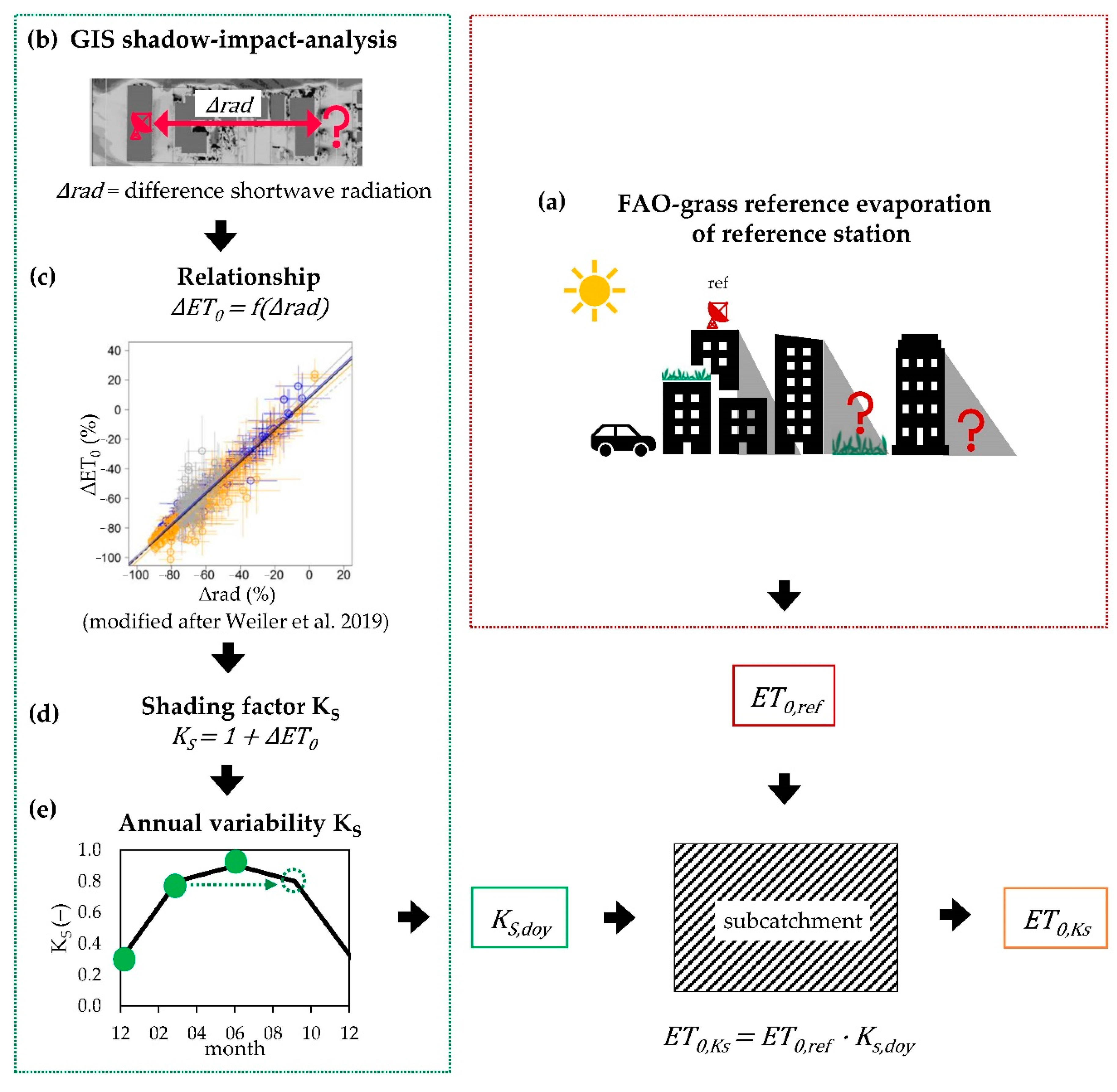
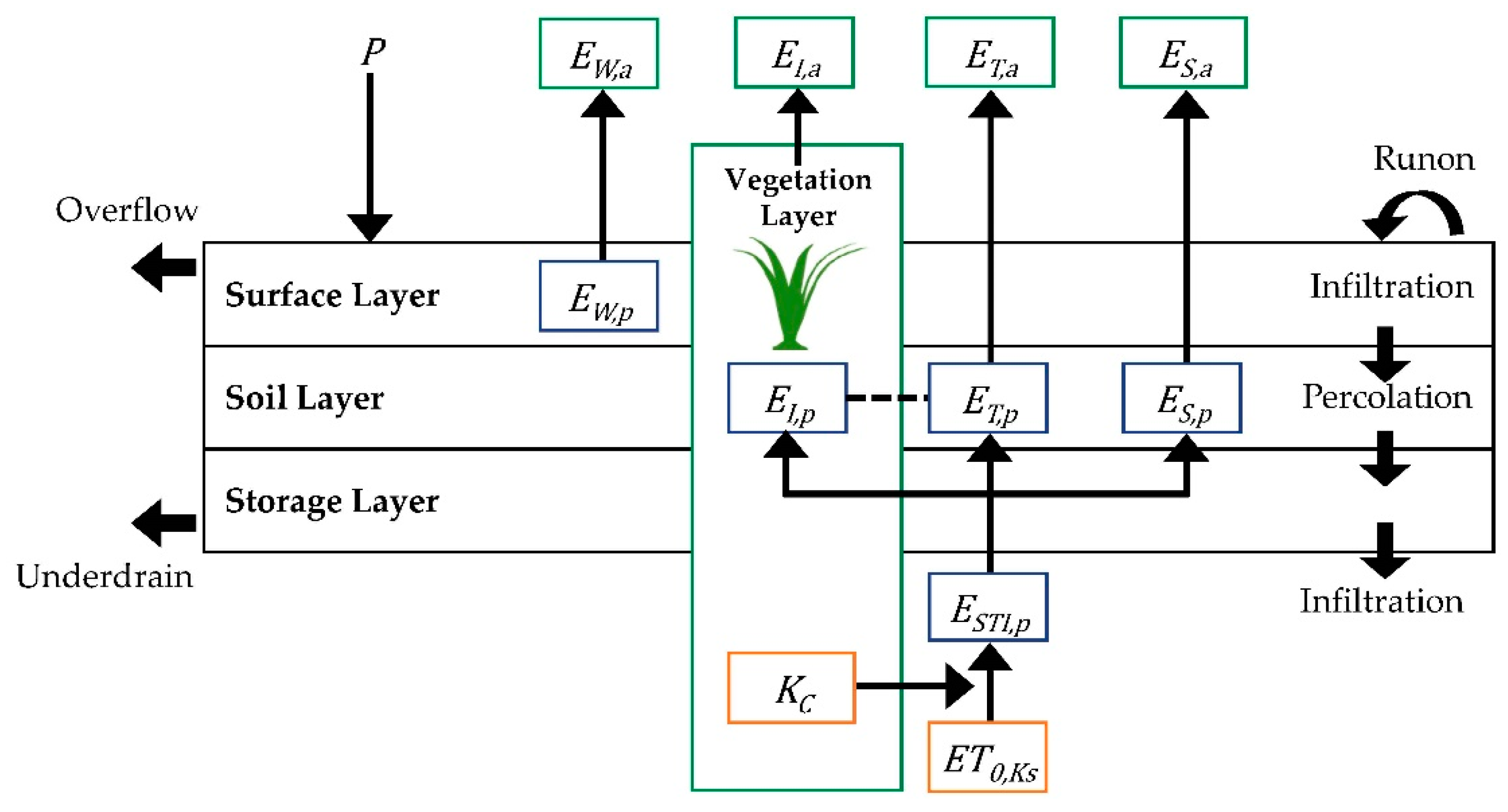
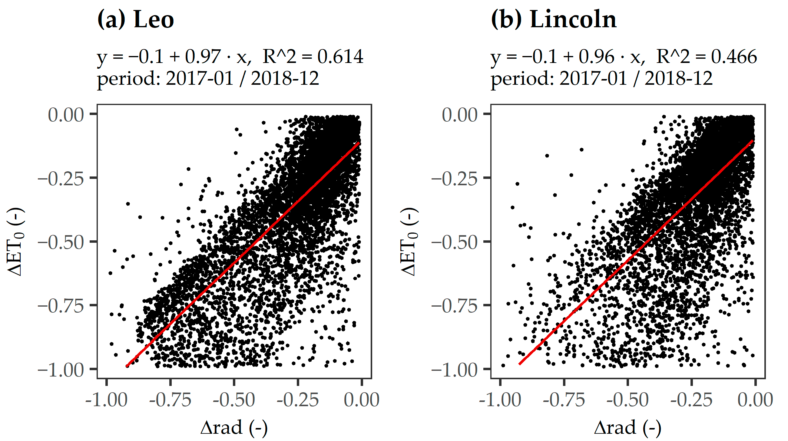
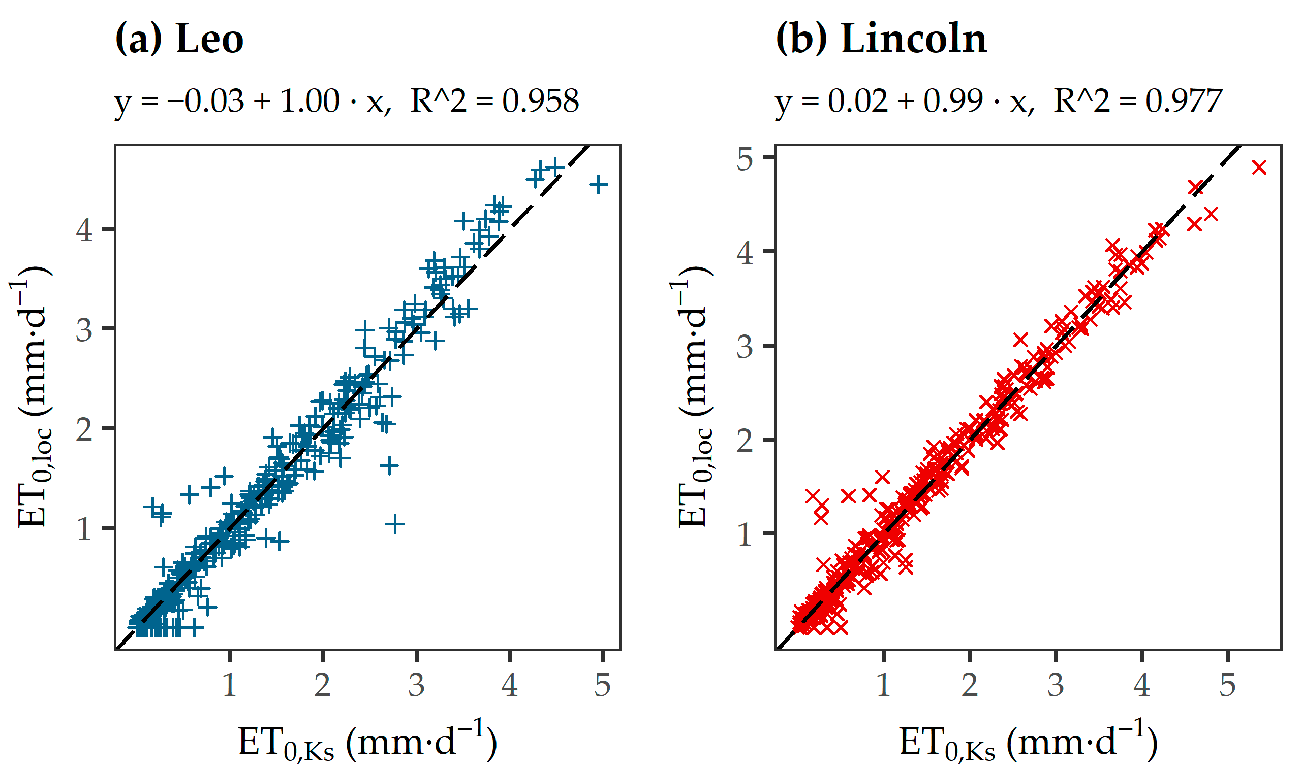
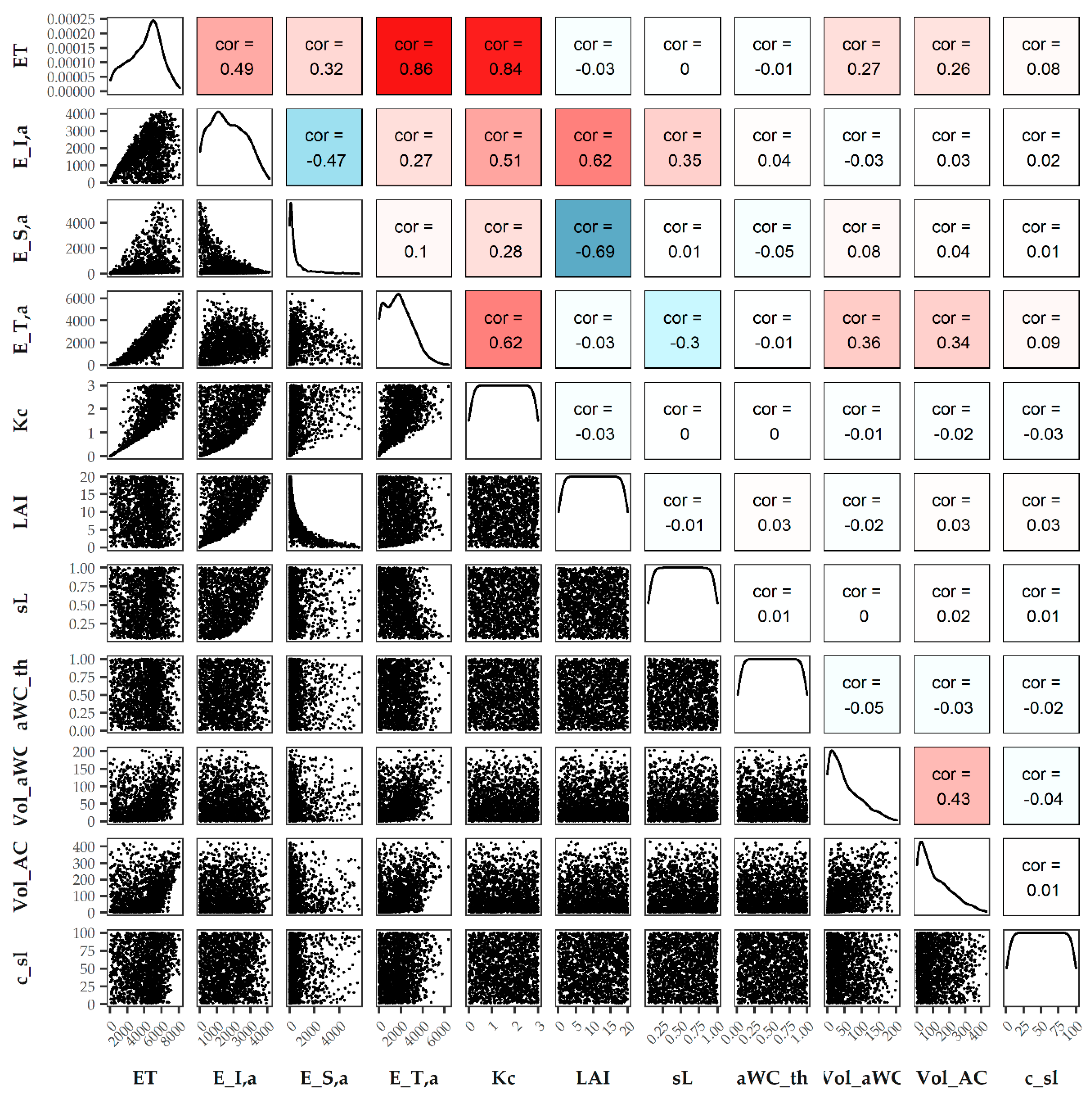
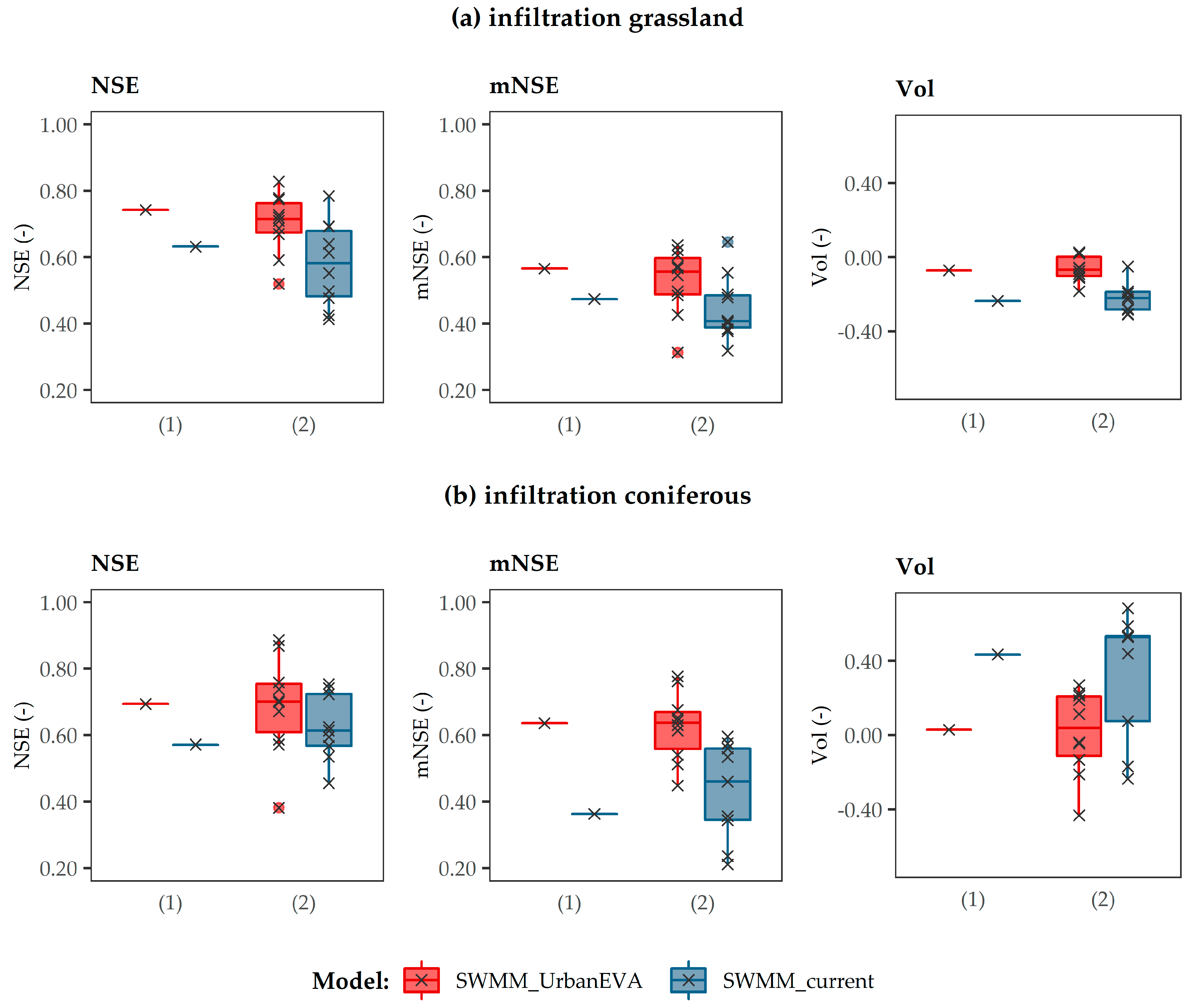
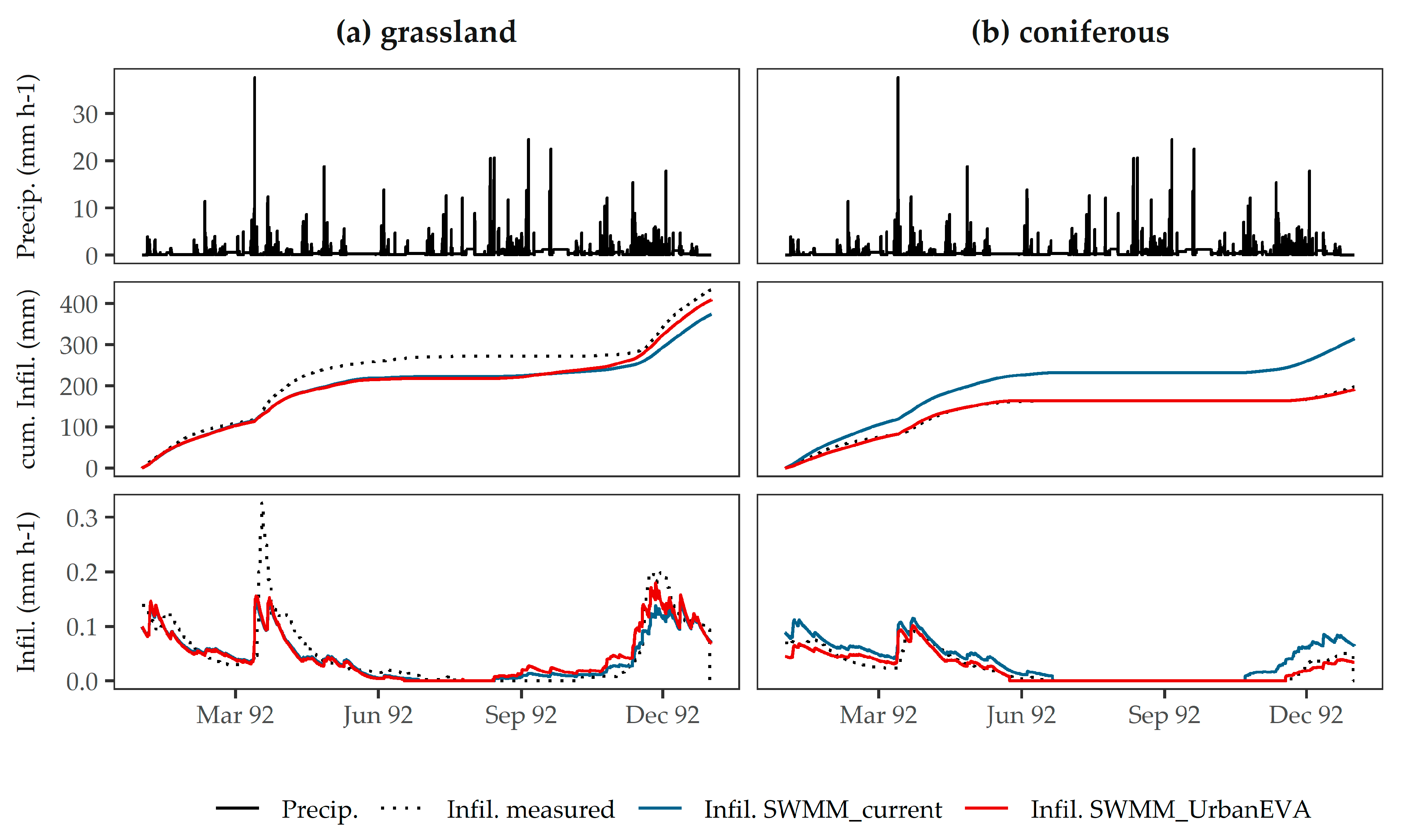
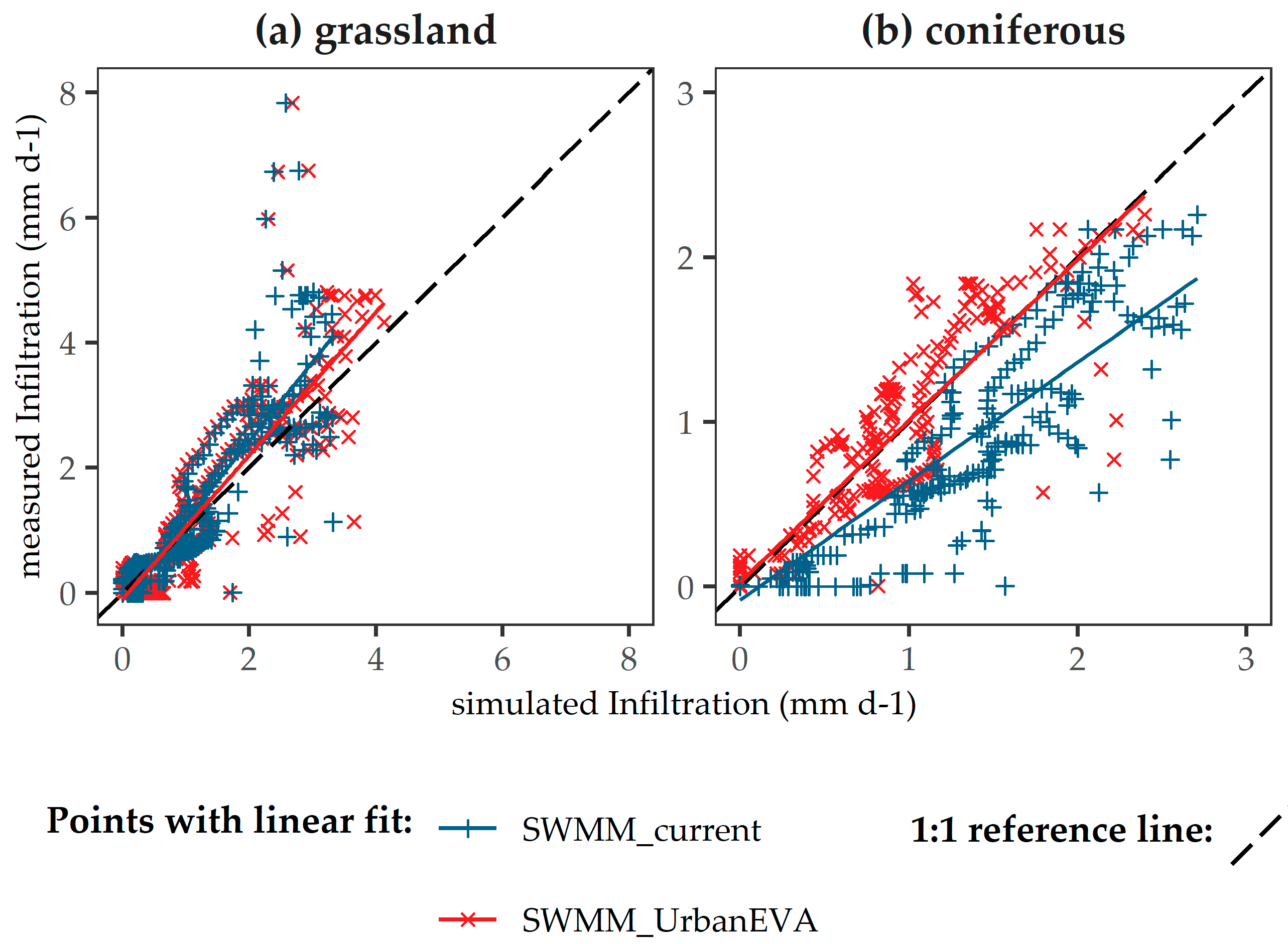
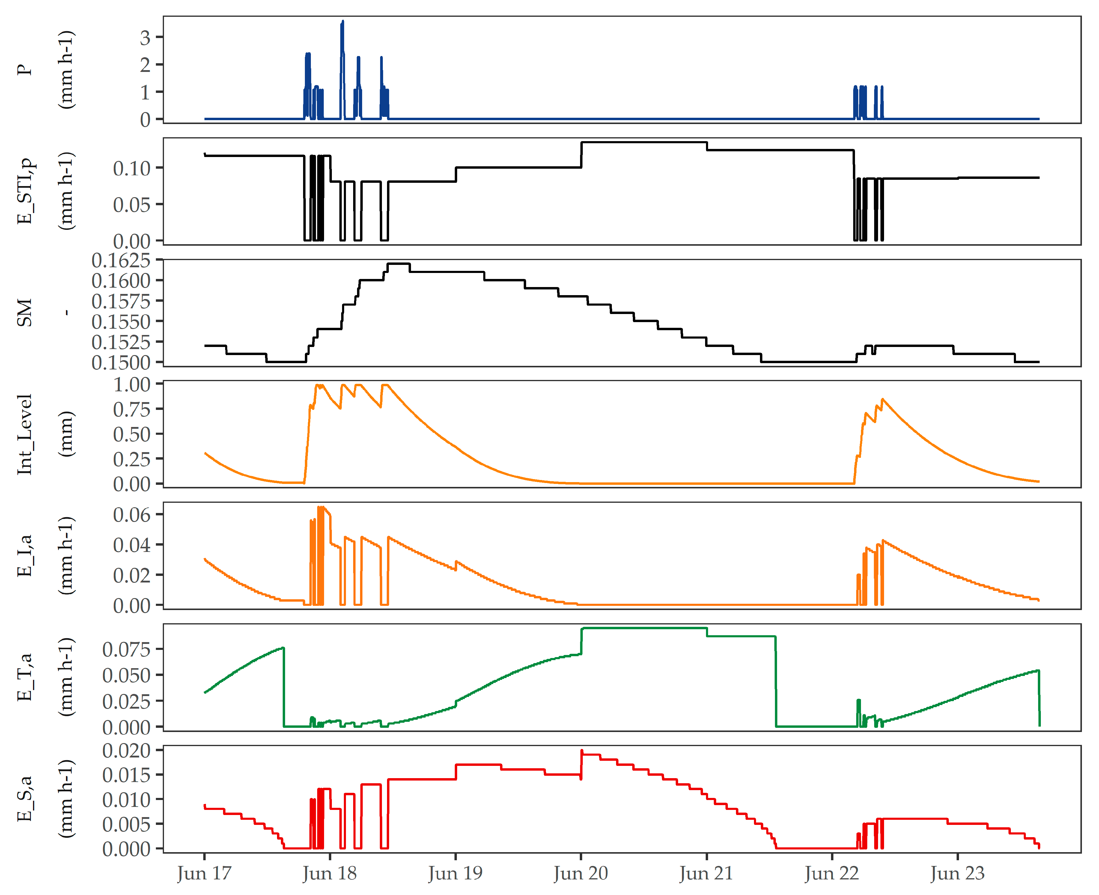
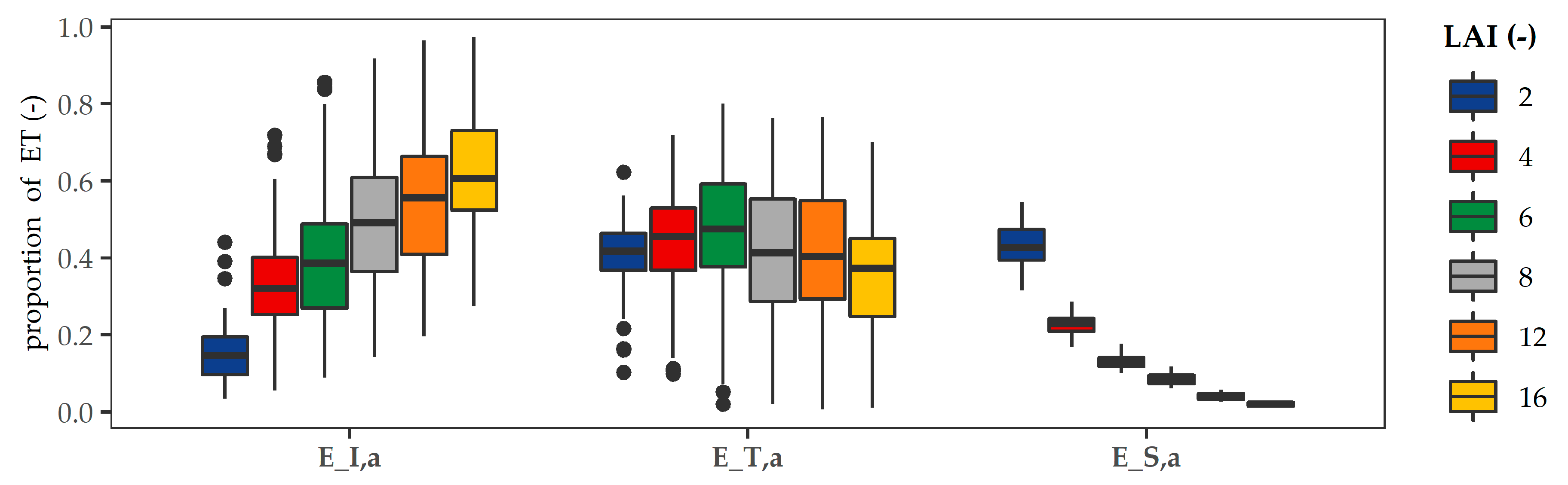
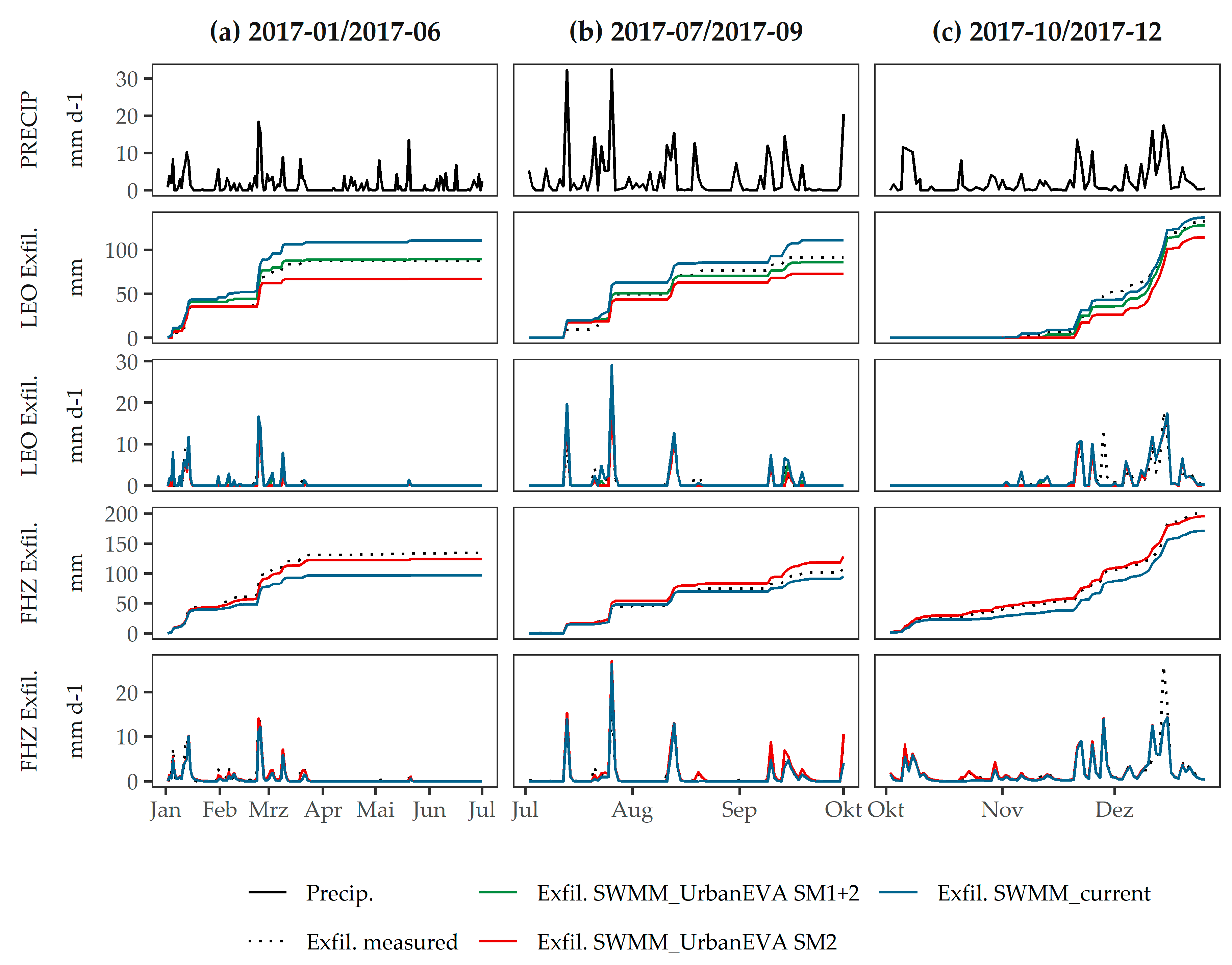
Table 1.
Mean annual totals for precipitation and of the locations under consideration. The years in brackets indicate the analyzed periods.
Table 1.
Mean annual totals for precipitation and of the locations under consideration. The years in brackets indicate the analyzed periods.
| Parameter | Unit | St. Arnold | Geo | Leo | Lincoln |
|---|---|---|---|---|---|
| (1966–2008) | (2017–2018) | (2017–2018) | (2017–2018) | ||
| Precipitation | mm·a−1 | 793 | 596 | 691 | 647 |
| ET0 | mm·a−1 | 460 | 648 | 490 | 524 |
Table 2.
Overview study set up.
| Parameter | STEP 1: Shading (SM1) | STEP 2: ET Vegetation (SM2) | STEP 3 BGI (SM1 + SM2) | |
|---|---|---|---|---|
| Sensitivity | Calibration | |||
| Location | Münster (“Leo” and “Lincoln”) | St. Arnold | Münster (“Leo” and “FHZ”) | |
| Reference station | “Geo” | St. Arnold (no shading) | “Geo” | |
| Measurement | ET0,loc “Leo” and “Lincoln” | infiltration grassland/coniferous | exfiltration green roofs “Leo” and “FHZ” | |
| Timestep | 5 min | daily | 5 min | |
| Methods | - | LHS | SCEUA | SCEUA |
| Period | 2017 | 1989/1999 | 1989/1999, 1989, …, 1999 | 2017-01/2017-03; 2017-04/2017-06; 2017-02-21/2017-02-27; 2017-03-07/2017-03-17 |
| Varied input parameters | KS,spring, KS,summer, KS,winter, (see Table 4) | all LID + SWMM-UrbanEVA variables, (see Table 5) | KC, SoDepth, Por, WP, c_sl (see Table 7) | KC, Por, WP, c_sl, FCoef, FEx (see Table 7) |
| Evaluated result parameters | “Leo” and “Lincoln” | ET, EI,a, ET,a, ES,a | infiltration grass./ conif. | exfiltration green roofs “Leo” and “FHZ” |
| Goodness-of-fit | NSE, mNSE, Vol | |||
Table 3.
Goodness-of-fit criteria under consideration.
| Goodness-of-Fit Criterion | Formula | Equation No. |
|---|---|---|
| Nash-Sutcliffe model efficiency | (43) | |
| Modified Nash-Sutcliffe model efficiency | (44) | |
| Volume Error | (45) |
= modelled result; = observed result.
Table 4.
Reduction in shortwave radiation () and resulting -values used for the estimation of . All values have been calculated for spring equinox as well as winter and summer solstice.
Table 4.
Reduction in shortwave radiation () and resulting -values used for the estimation of . All values have been calculated for spring equinox as well as winter and summer solstice.
| Parameter | Unit | Leo | Lincoln | |||||
|---|---|---|---|---|---|---|---|---|
| Spring | Summer | Winter | Spring | Summer | Winter | |||
| (i) | - | −0.15 | −0.12 | −0.25 | −0.13 | −0.07 | −0.12 | |
| (ii) | - | 0.75 | 0.78 | 0.66 | 0.78 | 0.84 | 0.79 | |
Table 5.
LID parameter ranges for sensitivity analysis and model calibration. (grey = fixed parameter, black = varied parameter).
Table 5.
LID parameter ranges for sensitivity analysis and model calibration. (grey = fixed parameter, black = varied parameter).
| Parameter | Unit | Min | Max | Reference | ||
|---|---|---|---|---|---|---|
| vegetation | crop factor | Kc | - | 1 | 3 | [32] |
| leaf area index | LAI | - | 1 | 16 | [36] | |
| leaf storage coefficient | SL | - | 0 | 1 | - | |
| aWCthreshold | aWC-th | - | 0 | 1 | - | |
| surface | surface storage | SuStor | mm | 1 | 10 | site specific |
| surface roughness | SuManN | s·m−1/3 | 0.001 | 0.8 | [87] | |
| surface slope | SuSlope | % | 0 | 6 | site specific | |
| soil | soil depth | SoDepth | mm | 1 | 2000 | site specific |
| porosity | Por | - | 0.22 | 0.65 | [88] | |
| field capacity | FC | - | 0.21 | 0.21 | [88] | |
| wilting point | WP | - | 0 | 0.20 | [88] | |
| conductivity | cond | mm·h−1 | 0.25 | 360 | [87] | |
| conductivity slope | c_sl | - | 1 | 100 | [34] | |
| suction head | SucH | mm | 49 | 320 | [34] | |
| storage | storage height | StHeight | mm | 1 | 5000 | site specific |
| void ratio | VoidR | - | 0 | 1 | [88] | |
| seepage rate | SR | mm·h−1 | 0.25 | 360 | [87] | |
Table 6.
Comparison of out of local measurements () with the -modified of the reference station () for 2017.
Table 6.
Comparison of out of local measurements () with the -modified of the reference station () for 2017.
| Month in 2017 | Leo | Lincoln | ||||||
|---|---|---|---|---|---|---|---|---|
| ET0,loc | ET0,Ks | Diff. | ET0,loc | ET0,Ks | Diff. | |||
| (mm) | (mm) | (mm) | (%) | (mm) | (mm) | (mm) | (%) | |
| January | 2.9 | 7.4 | 4.5 | 153.2 | 5.5 | 8.4 | 3.0 | 54.4 |
| February | 13.0 | 13.1 | 0.1 | 0.6 | 12.5 | 14.2 | 1.7 | 13.5 |
| March | 37.8 | 32.9 | −4.9 | −13.0 | 38.7 | 34.2 | −4.5 | −11.6 |
| April | 49.4 | 47.3 | −2.2 | −4.4 | 52.3 | 49.5 | −2.7 | −5.3 |
| May | 77.5 | 75.4 | −2.1 | −2.7 | 81.2 | 80.3 | −0.9 | −1.1 |
| June | 82.3 | 82.6 | 0.3 | 0.3 | 88.8 | 89.1 | 0.4 | 0.4 |
| July | 80.0 | 77.3 | −2.8 | −3.4 | 84.3 | 82.7 | −1.6 | −1.9 |
| August | 58.7 | 61.9 | 3.3 | 5.6 | 64.7 | 65.2 | 0.5 | 0.8 |
| September | 34.2 | 35.6 | 1.4 | 4.1 | 37.9 | 37.0 | −0.8 | −2.2 |
| October | 17.2 | 21.8 | 4.6 | 26.5 | 20.7 | 23.4 | 2.7 | 13.1 |
| November | 6.3 | 7.2 | 0.9 | 14.5 | 7.1 | 8.1 | 1.0 | 14.5 |
| December | 4.7 | 4.3 | −0.5 | −9.5 | 5.8 | 5.1 | −0.7 | −12.1 |
| ∑ | 464 | 467 | 3 | 1 | 499 | 497 | −2 | −0.4 |
Table 7.
LID parameters obtained from model calibration. (grey = fixed parameter, black = varied parameter).
Table 7.
LID parameters obtained from model calibration. (grey = fixed parameter, black = varied parameter).
| Parameter | Unit | Full Scale Lysimeter St. Arnold | Green Roofs | |||||||
|---|---|---|---|---|---|---|---|---|---|---|
| SWMM-UrbanEVA | SWMM-Current | |||||||||
| Grass | Conif. | Grass | Conif. | Leo | FHZ | |||||
| General | area | Area | M2 | 400 | 400 | 400 | 400 | 3 | 80 | |
| width | Width | m | 20 | 20 | 20 | 20 | 1 | 9 | ||
| initial saturation | InitSat | - | 0 | 0 | 0 | 0 | 0 | 0 | ||
| slope | Slope | % | 2 | 2 | 2 | 2 | 3 | 3 | ||
| SM1 | shading factor spring | KS,spring | - | 1 | 1 | - | - | 0.75 | 1 | |
| shading fact. summer | KS,summer | - | 1 | 1 | - | - | 0.78 | 1 | ||
| shading factor winter | KS,winter | - | 1 | 1 | - | - | 0.66 | 1 | ||
| SM2 | vegetation | crop factor | Kc | - | 1.04 | 1.56 | - | - | 1.80 | 1.14 |
| leaf area index | LAI | - | 2 | 11 | - | - | 3 | 3 | ||
| leaf storage coefficient | SL | % | 0.29 | 0.29 | - | - | 0.29 | 0.29 | ||
| aWCthreshold | aWC-th | % | 0.6 | 0.6 | - | - | 0.6 | 60 | ||
| gf scheme | gf | - | Table S1, no. 7 | |||||||
| surface | surface storage | SuStor | mm | 2 | 2 | 2 | 2 | 20 | 20 | |
| surface roughness | SuManN | s·m−1/3 | 0.1 | 0.1 | 0.1 | 0.1 | 0.1 | 0.1 | ||
| surface slope | SuSlope | % | 1 | 1 | 1 | 1 | 3 | 3 | ||
| soil | soil depth | SoDepth | mm | 1596 | 1639 | 1616 | 2331 | 150 | 60 | |
| porosity | Por | - | 0.48 | 0.57 | 0.46 | 0.50 | 0.29 | 0.40 | ||
| volume air capacity | VolAC | mm | 431 | 590 | 404 | 676 | 14 | 10 | ||
| field capacity | FC | - | 0.21 | 0.21 | 0.21 | 0.21 | 0.20 | 0.23 | ||
| wilting point | WP | - | 0.18 | 0.10 | 0.19 | 0.11 | 0.10 | 0.07 | ||
| volume avail. water cap. | VolaWC | mm | 35 | 180 | 32 | 233 | 15 | 10 | ||
| conductivity | cond | mm·h−1 | 250 | 250 | 250 | 250 | 61 | 27 | ||
| conductivity slope | c_sl | - | 40.6 | 28.4 | 36.5 | 34.8 | 63.8 | 37.6 | ||
| suction head | SucH | mm | 58 | 58 | 58 | 58 | 58 | 58 | ||
| storage | storage height | StHeight | mm | 3000 | 3000 | 3000 | 3000 | 25 | 30 | |
| void ratio | VoidR | - | 0.27 | 0.27 | 0.27 | 0.27 | 0.75 | 0.30 | ||
| seepage rate | SR | mm·h−1 | 250 | 250 | 250 | 250 | 0 | 0 | ||
| drain | flow coefficient | FCoef | 1·h−1 | - | - | - | - | 53 | 43 | |
| flow exponent | FEx | - | - | - | - | - | 0.9 | 0.2 | ||
| offset | Off | mm | - | - | - | - | 0 | 0 | ||
Table 8.
Mean (mean), standard deviation (SD) and variation coefficient (VarC) for last population of calibration-runs for grassland and coniferous.
Table 8.
Mean (mean), standard deviation (SD) and variation coefficient (VarC) for last population of calibration-runs for grassland and coniferous.
| Parameter | Unit | Grassland | Coniferous | |||||
|---|---|---|---|---|---|---|---|---|
| Mean | SD | VarC | Mean | SD | VarC | |||
| crop factor | Kc | - | 1.05 | 0.17 | 16% | 1.57 | 0.19 | 15% |
| soil depth | SoDepth | mm | 1463 | 146 | 10% | 1555 | 268 | 17% |
| porosity | Por | - | 0.50 | 0.02 | 4% | 0.55 | 0.04 | 8% |
| volume air capacity | VolAC | mm | 431 | 40 | 9% | 545 | 113 | 21% |
| wilting point | WP | - | 0.18 | 0.02 | 9% | 0.10 | 0.02 | 21% |
| volume available water capacity | VolaWC | mm | 29 | 20 | 67% | 167 | 39.5 | 24% |
Table 9.
Performance criteria for measured and modeled infiltration of calibrated models in 1992.
| Parameter | Unit | SWMM-UrbanEVA | SWMM-Current | ||
|---|---|---|---|---|---|
| Grassland | Coniferous | Grassland | Coniferous | ||
| NSE | - | 0.74 | 0.87 | 0.73 | 0.47 |
| mNSE | - | 0.59 | 0.75 | 0.63 | 0.41 |
| Vol | - | −0.06 | −0.14 | −0.04 | 0.59 |
Table 10.
ET partitioning validation for different species. (frac. = fraction of ET, abs. dev. = absolute deviation, rel. dev. = relative deviation).
Table 10.
ET partitioning validation for different species. (frac. = fraction of ET, abs. dev. = absolute deviation, rel. dev. = relative deviation).
| Species | LAI | Literature | SWMM-UrbanEVA | ||||||||||
|---|---|---|---|---|---|---|---|---|---|---|---|---|---|
| EI,a/ET | ET,a/ET | ES,a/ET | EI,a/ET | ET,a/ET | ES,a/ET | ||||||||
| Frac. | Frac. | Frac. | Frac. | Abs. Dev. | Rel. Dev | Frac. | Abs. Dev. | Rel. Dev | Frac. | Abs. Dev. | Rel. Dev | ||
| (-) | (-) | (-) | (-) | (-) | (-) | (-) | (-) | (-) | (-) | (-) | (-) | ||
| grassland | 2 | 0.25 1 | 0.50 1 | 0.25 1 | 0.15 | −0.10 | −0.60 | 0.42 | −0.08 | −0.19 | 0.43 | 0.18 | 0.72 |
| pine | 8 | 0.45 2. | 0.47 2 | 0.08 2 | 0.49 | 0.04 | 0.09 | 0.42 | −0.05 | −0.07 | 0.09 | 0.01 | 0.13 |
| spruce | 12 | 0.50 3 | 0.44 3 | 0.06 3 | 0.56 | 0.06 | 0.12 | 0.40 | −0.04 | −0.10 | 0.04 | −0.02 | -0.33 |
Table 11.
Performance criteria of the different models for the green roofs “Leo” and “FHZ”. The analysis was done with a daily timestep.
Table 11.
Performance criteria of the different models for the green roofs “Leo” and “FHZ”. The analysis was done with a daily timestep.
| Model | (a) Calibration (2017-01 and 2017-06) | (b) Validation 1 (2017-07 and 2017-09) | (c) Validation 2 (2017-10 and 2017-12) | 2017 | |||||||||
|---|---|---|---|---|---|---|---|---|---|---|---|---|---|
| NSE | mNSE | Vol | NSE | mNSE | Vol | NSE | mNSE | Vol | NSE | mNSE | Vol | ||
| Leo | UE SM1+2 | 0.84 | 0.71 | 0.01 | 0.85 | 0.72 | −0.06 | 0.71 | 0.61 | −0.01 | 0.79 | 0.69 | −0.02 |
| UE SM2 | 0.82 | 0.69 | −0.24 | 0.82 | 0.70 | −0.21 | 0.72 | 0.62 | −0.11 | 0.78 | 0.68 | −0.17 | |
| current | 0.79 | 0.65 | 0.25 | 0.83 | 0.73 | 0.21 | 0.70 | 0.60 | 0.06 | 0.77 | 0.67 | 0.15 | |
| FHZ | UE SM1+2 | - | - | - | - | - | - | - | - | - | - | - | - |
| UE SM2 | 0.95 | 0.81 | −0.08 | 0.88 | 0.78 | 0.18 | 0.81 | 0.78 | −0.03 | 0.89 | 0.81 | 0.00 | |
| current | 0.90 | 0.74 | −0.28 | 0.89 | 0.79 | −0.13 | 0.80 | 0.74 | −0.15 | 0.87 | 0.78 | −0.18 | |
Publisher’s Note: MDPI stays neutral with regard to jurisdictional claims in published maps and institutional affiliations. |
© 2021 by the authors. Licensee MDPI, Basel, Switzerland. This article is an open access article distributed under the terms and conditions of the Creative Commons Attribution (CC BY) license (http://creativecommons.org/licenses/by/4.0/).
Share and Cite
MDPI and ACS Style
Hörnschemeyer, B.; Henrichs, M.; Uhl, M. SWMM-UrbanEVA: A Model for the Evapotranspiration of Urban Vegetation. Water 2021, 13, 243. https://doi.org/10.3390/w13020243
AMA Style
Hörnschemeyer B, Henrichs M, Uhl M. SWMM-UrbanEVA: A Model for the Evapotranspiration of Urban Vegetation. Water. 2021; 13(2):243. https://doi.org/10.3390/w13020243
Chicago/Turabian StyleHörnschemeyer, Birgitta, Malte Henrichs, and Mathias Uhl. 2021. "SWMM-UrbanEVA: A Model for the Evapotranspiration of Urban Vegetation" Water 13, no. 2: 243. https://doi.org/10.3390/w13020243
Note that from the first issue of 2016, this journal uses article numbers instead of page numbers. See further details here.