
A Simplified Model for Predicting the Effectiveness of Bioswale’s Control on Stormwater Runoff from Roadways

1
Department of Civil Engineering, Southern Illinois University Edwardsville, Edwardsville, IL 62026, USA
2
Water Resource Engineer, Stantec Consultant Engineering Inc., St. Louis, MO 63026, USA
3
Department of Civil Engineering, University of Akron, Akron, OH 44325, USA
*
Author to whom correspondence should be addressed.
Water 2021, 13(20), 2798; https://doi.org/10.3390/w13202798
Submission received: 14 July 2021
/
Revised: 18 August 2021
/
Accepted: 20 August 2021
/
Published: 9 October 2021
(This article belongs to the Section Urban Water Management)
Abstract
:Bioswales are commonly constructed along roadways to control stormwater runoff. Many factors can affect the performance of a bioswale such as the size of the bioswale and its associated drainage area, rainfall characteristics, site conditions, soil properties, and deterioration of the bioswale’s condition over usage. Transportation agencies and engineering communities need a reliable and convenient method for predicting the effectiveness of bioswale. Although available software tools can be used to model and analyze design options, input values for a large number of variables and highly skilled modelers are required to handle these sophisticated modeling tools. The objective of this study was to develop a simplified and easy-to-use mathematical model for predicting the effectiveness of bioswales through empirical predictions of stormwater runoff as a function of four key parameters: area ratio (bioswale surface area to its drainage service area), rainfall depth, rainfall intensity, and sediment accumulation (build-up) on bioswale’s surface area. A PCSWMM model was developed to simulate the physical conditions of a field-scale bioswale. This PCSWMM tool was also used to simulate an idealized (conceptual) catchment model that represents common highway geometries and characteristics. A total of 72 scenarios were simulated on various combinations of the four studied parameters: area ratio (9%, 13%); rainfall depth (2.54, 5.08, 7.62, 10.16 cm); rainfall intensity (2.54, 5.08, 10.16 cm/h); and sediment accumulation (0, 0.25, 1.78 cm). Half of the total scenarios (i.e., 36 scenarios) were used to develop a new simplified mathematical model, and the other 36 scenarios were used to calibrate and validate this newly developed model. The analysis revealed a reasonable correlation (R2 = 0.967) between modelled predictions and PCSWMM-simulated results, indicating the newly developed mathematical model can serve as an adequate alternative for simulating bioswales’ performance for stormwater runoff control.
1. Introduction
Best Management Practices (BMPs) [1,2,3,4,5,6,7,8,9,10,11,12,13,14,15,16,17,18,19,20,21,22,23,24,25,26,27,28,29,30,31] have been widely used for reducing the adverse impacts of stormwater runoff on receiving waters [2,16,26]. BMPs can be used to treat stormwater for the reduction of pollutants in the runoff. BMPs can also be used to lower the quantity of runoff, therefore, to reduce pollution loading on receiving waters. One of the most commonly used BMPs is bioswales. As a linear BMP, bioswales are very suitable to be installed along roadways to control stormwater runoff from road surfaces, regardless of the roads being urban roads or rural highways [12,17,18,29].
The effectiveness of bioswales for stormwater runoff control is affected by many factors such as drainage service area, rainfall depth, rainfall intensity, surface vegetative cover, and soil infiltration rates [18,19,20]). Poresky et al. (2011) [26] reported that, based on monitored performance, stormwater volume reduction by bioswales ranged from 35% to 65%. Geosyntec (2008) [8] and Caltrans (2004) [5] indicated that the performances of bioswales are affected by specifics of the installed units, such as sizes of the bioswales, rainfall characteristics, geometrical and topographical conditions of the sites, properties of the soils, vegetation of the surface cover, and the physical condition and age of the bioswales at the time the BMP performance was evaluated. It was recognized that most of the bioswales evaluated by Poresky et al. (2011) [26] were installed during 1980s or 1990s. Therefore, their reported 35–65% runoff reductions are expected to be lower than the percent runoff reduction performance when the bioswales are newly installed [7]. The uncertainty about the effect of the age of bioswale on runoff reduction was not reported by Clary et al. (2012) [7].
Transportation administration agencies and engineering communities need an easy-to-use, reliable, and convenient tool for adequately predicting the effectiveness of a bioswale’s control on stormwater runoff from roadways, so that cost-effective measures of stormwater runoff control and pollution reduction can be developed and implemented. However, such a tool presently is not available [23]. Transportation agencies and engineers can use modeling software tools such as the Storm Water Management Model (SWMM) to build a physical model and simulate project specifics and analyze design options. Such a modeling approach requires appropriately pre-defined input values for an extensive number of variables (e.g., more than 20 variables for SWMM) and highly skilled and experienced modelers with specialized engineering or hydrologic backgrounds to handle such a sophisticated modeling tool.
The objective of the study described in this paper was to develop a simplified, reliable, and easy-to-use mathematical model for predicting the effectiveness of a bioswale’s control on stormwater runoff from roadways.
A large number of studies revealed that the ratio of the bioswale’s surface area to its drainage service area (area ratio, AR), rainfall depth (RD), rainfall intensity (RI), and sediment accumulation (SA) or build-up on bioswale’s surface area are among the most important factors affecting a bioswale’s performance [4,6,9,11,22,32] because AR and rainfall (RD, RI) determine the amount of stormwater run onto a given bioswale and accumulated sediments directly affect the infiltration rate of the bioswale’s medium [3]. The simplified mathematical model by this study was intended to establish empirical predictions of stormwater runoff as a function of four key parameters: AR, RD, RI, and SA.
2. Systematic Approach to Develop a Simplified Mathematical Model
To develop a simplified mathematical model, the following approach was taken:
- A field-scale bioswale testing facility was designed and constructed.
- A Personal Computer Storm Water Management Model (PCSWMM) numerical model based on the physical conditions of this field-scale bioswale was developed. PCSWMM is derived from SWMM. Although software tools have the same hydraulic and hydrologic analysis capability, PCSWMM offers enhanced graphic user interfaces that are much improved from USEPA SWMM 5. PCSWMM was chosen for this research work.
- The PCSWMM model was validated using the experimental data from testing the field-scale bioswale [23]
- An idealized (conceptual) catchment model that represents typical highway geometries and characteristics was developed for PCSWMM modeling and simulations.
- A matrix of simulated conditions of the studied factors (i.e., AR, RD, RI, SA) was developed.
- Results from half of PCSWMM’s simulated scenarios were used to develop a simplified mathematical model for predicting the bioswale’s control of stormwater runoff.
- The newly developed mathematical model was used to predict the bioswale’s control of stormwater runoff, which was compared to results from the second half of the PCSWMM-simulated scenarios.
- The applications of the newly developed mathematical model were discussed.Each of the above tasks and components are discussed in detail in the following sections.
3. Field-Scale Bioswale Testing Facility
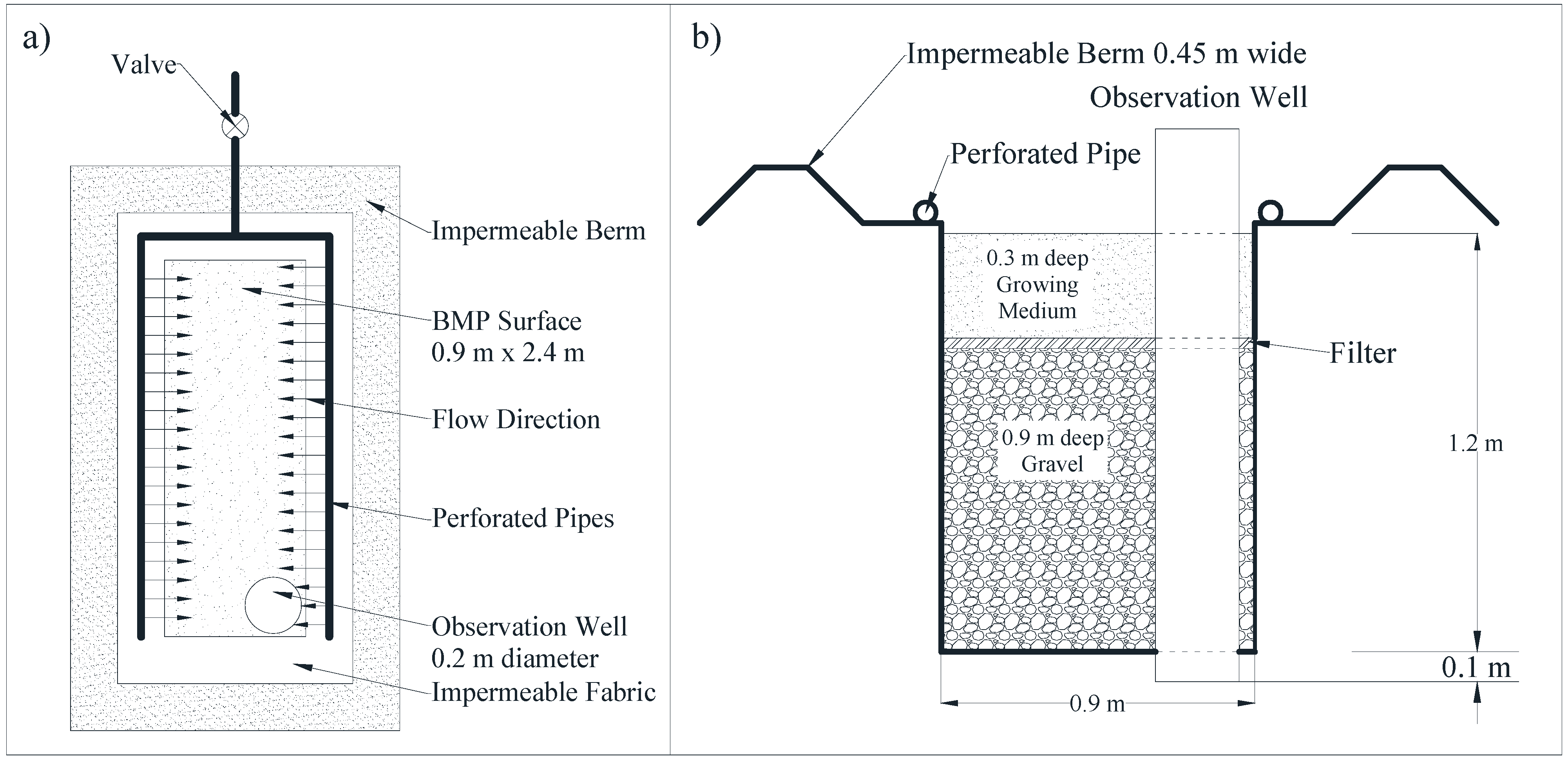
Set-up and physical conditions of the field-testing facility: Three testing units of bioswale were constructed on the campus of Southern Illinois University Edwardsville (SIUE) (Osouli et al., 2017b). The plan and section views of one testing unit are illustrated in Figure 1. Each testing unit consists of a trench of 1.2 m (4 ft) in depth, 2.4 m (8 ft) in length and 0.9 m (3 ft) in width. The three testing units are separated by 5 m of in-between spacing. Each trench was filled with 0.9 m (3 ft) of aggregates of not more than 2.54 cm (1 inch) in particle size, which were placed in loose condition. After a non-woven geofabric filter layer was placed on top of the aggregates, each trench was filled with growth medium of 0.3 m (1 ft) to its surface level. The medium was obtained from a local market in Edwardsville, IL.
USGS data indicate that native soils at this SIUE testing site are mainly sandy lean clay. The infiltration rate of the native soil was measured at a depth of 1.3 m below the ground surface (Figure 1b) by a Turf-Tec infiltrometer immediately after excavation of the site before placement of the aggregate. Major properties of the materials used in bioswale testing units are summarized in Table 1.
Operation of the Testing Facility
Rainfalls and Stormwater Runoff (i.e., run-on to the tested bioswale units): the bioswale performance was tested by applying controlled amounts and flow rates of water to the surface of each unit, which correspond to the tested rainfall conditions.
The Illinois Environmental Protection Agency (IEPA) expects on-site control of stormwater runoff resulting from the first 2.54 cm (1 inch) of rainfall, which represents the 90th percentile of total rainfall depth from rainfalls of 24 h duration in Illinois [14]. For this total rainfall depth, the Intensity-Duration-Frequency (IDF) data of Southwest Illinois, where SIUE campus is located, are used [13] to obtain rainfall intensities under several rainfall returns for this study. Three rainfall return frequencies (10 year, 2 year, and 9 month) were chosen to develop rainfall intensities and durations that correspond to the total rainfall depth of 2.54 cm (1 inch), which are shown in Table 2. Based on a drainage area of 15.2 m (50 ft) in length and 2.44 m (8 ft) in width for each bioswale unit, and a rainfall depth of 2.54 cm (1 inch), the amount of water for each bioswale unit was 945 L.
Applying Stormwater to Bioswale Units: The amount of water shown in Table 2 was pumped to each bioswale unit through a piping system. The flow rates of the applied water were controlled by a valve and a flow meter, and were recorded throughout the testing. The water was distributed through perforated pipes that were installed at surface level along two longitudinal sides of the bioswale as shown in Figure 1. In the process of water infiltration into the growth medium, when the standing water build-up was 40 mm higher than the surface level of the growth medium, the standing water was pumped out and discarded. The quantity of the pumped-out water was recorded and was taken as the runoff from the tested bioswale unit.
The water infiltration process along the vertical direction of the bioswale was monitored by recording water levels in an observation well, which was a 0.2 m diameter of perforated pipe installed along the entire depth of each bioswale as shown in Figure 1b. The recording was conducted by both a HOBO U20L sensor (for both depth and temperature of the water) installed at the bottom of the observation well, and by manual measurement of water levels in the well. The monitoring covered the entire period until the water in the observation well completely drained into the soils at the bottom of the well.
Applying Sediments to Bioswale Units: to evaluate the impact of sediment build-up on the bioswale’s performance, various amounts of sediments were applied on the surface of the growth medium. The amounts of the sediments were chosen by using the unversisal soil loss equation (USLE) method shown in Equation (1) [21].
where A is average annual soil loss (kg/m2/Year), R is rainfall-runoff erosivity factor, K is soil erodibility factor, LS is length-slope factor, C is cover-management factor, and P is support practice factor. The input values of these parameters were selected from technical references [31] that are appropriate for the conditions of the site in the Madison county of Illinois [23,24]. For soil losses along roadways, almost the whole amount is from the fore-slope and level areas off the roads, and a minimal amount is from the paved surfaces of roads. The USLE calculation for this study assumed that there is no atmospheric deposition of sediments or washed-off sediments from hillsides or mountains to the roads [28].
The USLE calculation indicated that soil loss from a typical developed area was 0.19 kg/m2/year. In comparison, the soil loss for the Madison County of Illinois that was specified by Madison County Soil and Water Conservation District (SWCD) and the typical soil loss in stabilized small watershed areas with fine-textured soils that was specified by the National Conservation District Employees Association (NCDEA) was 0.22 kg/m2/year. For this study, a soil loss of 0.19 kg/m2/year was used. Based on the drainage area for the tested bioswale, it is expected that newly built, 2-year-old, and 10-year-old of bioswales would have sediment build-ups of 0 cm, 0.25 cm, and 1.78 cm on the surface of the growth medium, respectively [23]. For the field testing, the simulated sediment build-ups were prepared from natural soils taken at the study site, which were sieved by No. 8 sieve. Such prepared soils were placed evenly and loosely atop the growth medium to various thicknesses to simulate the aging of the bioswale. The infiltration rate of these three sediment build-ups were measured by a Turf-Tec infiltrometer, and were found to be 181.2 cm/h, 54.4 cm/h, and 19.1 cm/h, respectively.
To provide an easy-to-use term for facilitating technical comparison, instead of using thickness of accumulated sediments, the travel time (TT) that water takes to pass through the thickness of the sediment layer is used to quantity the sediment build-up for the purpose of this paper. For example, at an infiltration rate of 19.1 cm/h for the 10-year-old bioswale, it takes water 5.6 min to pass through the 1.78 cm of sediment build-up layer. By this definition, the TTs for New, 2-year-old, and 10-year-old bioswales are 0 min, 0.3 min, and 5.6 min, respectively.
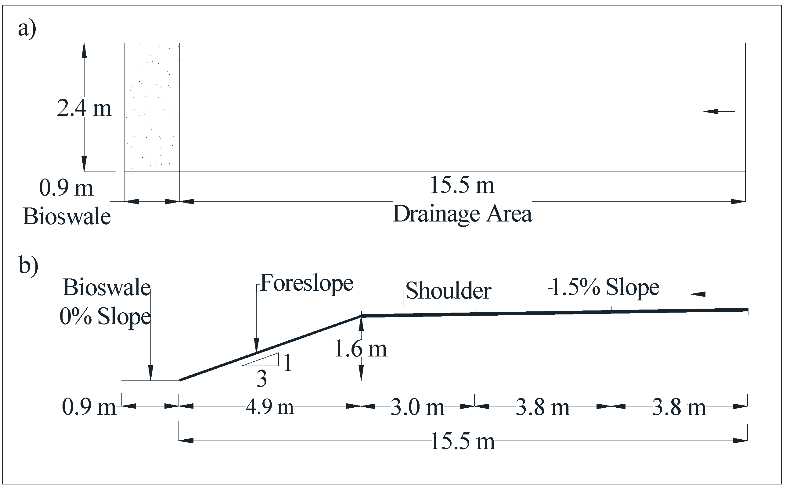
PCSWMM modeling of field-scale bioswale: A PCSWMM model (v.6.1.2015) was developed to simulate the SIUE field-scale bioswales. Runoffs were simulated with PCSWMM’s dynamic rainfall-runoff and Green-AMP method. The physical layout of field-scale bioswale for PCSWMM modeling is shown in Figure 2. The PCSWMM’s model layout consists of sub-catchment, conduits, and junctions. The input values of the modeled parameters are described hereafter. The drainage area (i.e., 15.5 m of horizontal length and 2.4 m of width, as shown in Figure 2) was set to have 100% imperviousness. The bioswale (i.e., the field-tested unit) was placed in the level area at 0.9 m of width (i.e., 0% slope in Figure 2), and is modeled with PCSWMM as the BMP unit. Further details are described in James et al. (2010), UDFCD (2008), Akhavan Bloorchian (2018), and Osouli et al. (2017a, 2017b, 2017c) [3,15,22,23,24,31]. The infiltration rates measured for the tested conditions were used in PCSWMM model simulations.
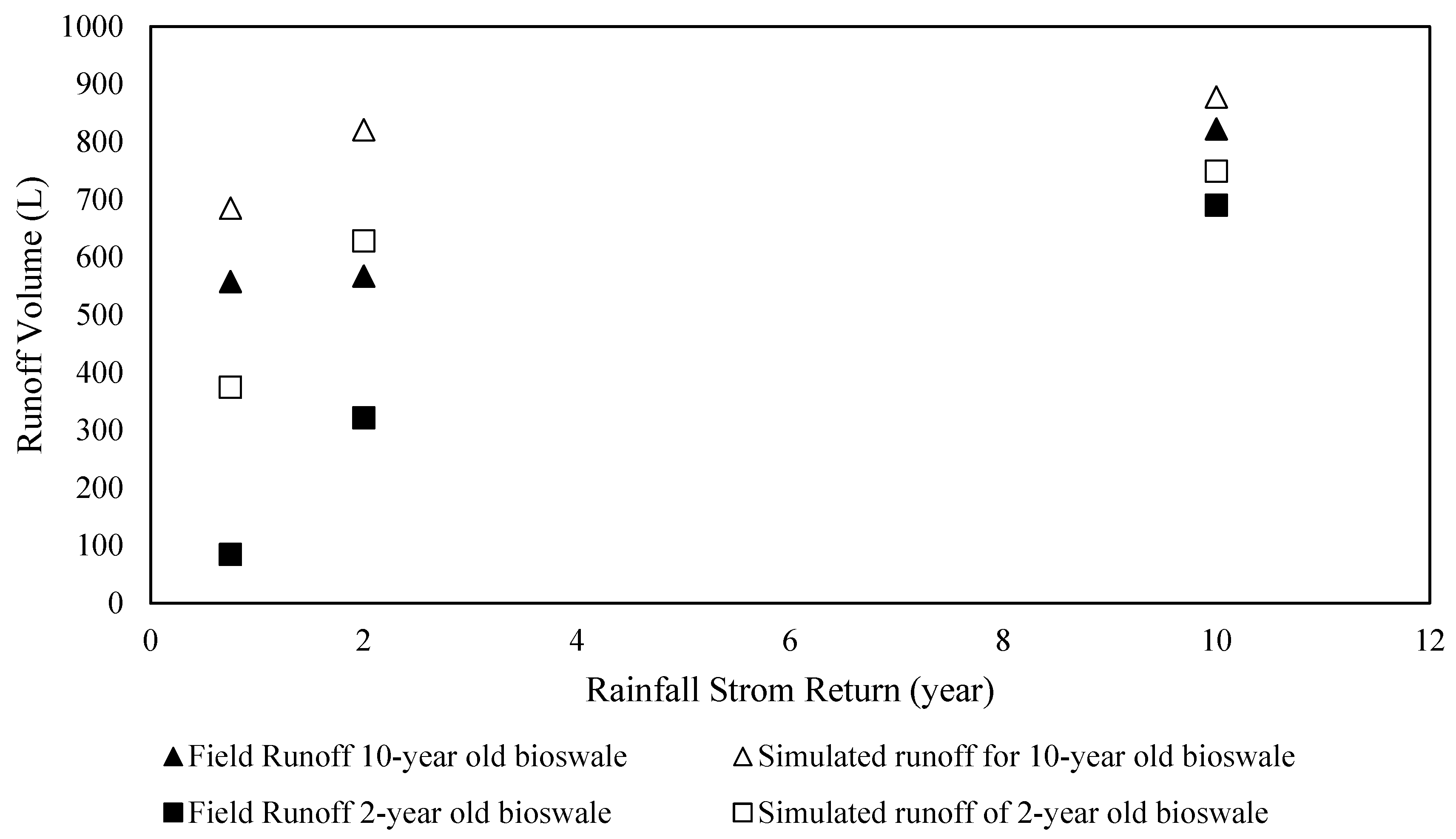
Validating the PCSWMM model: The simulated stormwater runoffs resulting from the PCSWMM modeling of field-tested bioswale units were compared to the measured stormwater runoffs from the field-tested bioswale unit. The field testing used 945 L of water as the total input of stormwater. For the newly-built bioswale, under all tested rainfall conditions shown in Table 2, both field-measured and PCSWMM-simulated results indicated zero runoffs. For 2-year-old and 10-year-old bioswales, as shown in Figure 3, under low rainfall events such as 9-month-return and 2-year-return, there were noticeable differences between field-measured and PCSWMM-simulated runoffs. For example, under 2-year-return of rainfall, for the 2-year-old bioswale, the field-measured runoff was 332 L, which was 47% lower than the PCSWMM-simulated runoff of 628 L; for the 10-year-old bioswale, the field-measured runoff was 568 L, which was 31% lower than the PCSWMM-simulated runoff of 821 L. However, under moderate rainfall event such as 10-year-return, the field-measured and PCSWMM-simulated runoffs matched with each other very well. In particular, for the 2-year-old bioswale, the field-measured runoff was 690 L, which is 8% lower than the PCSWMM-simulated runoff of 750 L; and for the 10-year-old bioswale, the field-measured runoff was 823 L, which is 6% lower than the PCSWMM-simulated runoff of 878 L. It was anticipated that field-measured runoffs were lower than the PCSWMM-simulated runoffs because of the unavoidable water loss from wetting the interior surface of pipes and parts, from water filling gaps in pumps, joints, and fittings, and from initial abstraction of the field system. As shown in Figure 3, the impact of such water loss on field measurement results were increasingly larger at lower rainfall events (e.g., 2-year-return vs. 10-year-return), because of the lower intensity and longer duration resulting small runoff volume. Even reasonable water loss would result in a relatively large percentage difference between field-measured and PCSWMM-simulated results. Given the storm runoff control was mainly concerned about runoff at moderate and large rainfall events, the 10-year-return rainfall event would provide more sound evaluation for validating the PCSWMM model. It also provides a better estimate in even smaller storm returns when the bioswale is aged. For example, for 10-year-old bioswale, the difference between field-measured and PCSWMM-simulated results for 2-year return and nine-month return are 46% and 22%, respectively, while for 2-year-old bioswale the difference becomes larger. Therefore, the PCSWMM model is accepted as validated and can be used for developing a simplified mathematical model for generalized stormwater runoff analyses.
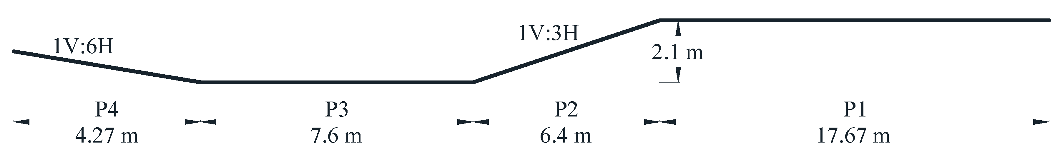
Developing an idealized (conceptual) catchment model: To develop a simplified mathematical model on stormwater runoff from bioswales along typical highways, an idealized (conceptual) catchment model was utilized to describe an eight-lane interstate highway and its right of way [1]. The prior-validated PCSWMM modeling tool was applied to this idealized catchment to conduct extensive simulations. This physical model sets four lanes on each direction with bioswales installed along both sides of the highway. Each lane was 3.6 m (12 ft) in width [1,10]. On each side of the highway, there is 3.05 m (10 ft) of shoulder. As shown in Figure 4, each bioswale along one side of the highway is to take stormwater runoff from an area of 17.7 m in width (58 ft = 4 lanes × 12 ft/lane + 10 ft shoulder, i.e., the P1 section in Figure 4). A 1.5% of cross-slope of the paved areas was used to drain runoff from highway lanes [1,10,18].
As shown in Figure 4, four subcatchment areas are considered in the modeling: paved road surface (P1), foreslope (P2), level ground (P3), and backslope (P4). The bioswale is placed within the area of the P3 subcatchment. The runoff from P1 discharges to P2, then to P3, and eventually to an outfall; or from P4 to P3, then to an outfall. For the analysis of this linear infrastructure, all of the subcatchments and associated analysis results are based on the unit length of highway.
The surface slopes of the foreslope (P2), level ground (P3), and backslope (P4) are set to be 33% (3H:1V), 0% (level), and 17% (6H:1V), respectively [25]. The embankment of the P2 area is set to be 2.1 m (7 ft) of elevation drop across the foreslope area. The bioswale unit in the P3 area is set to have a bottom width of 1.52 m (5 ft), 33% (3H:1V) side slope, 0.5% slope along the longitude direction of the bioswale, 0% imperviousness, 0.24 of Manning coefficient, 1.27 cm in the depth of depression storage in the bioswale, 30 cm maximum allowed depth of storage, and vegetative volume fraction of 0.2 [22,23]. For this study, the surface cover of unpaved areas was set as turf grass cover, which is typically found in Midwest USA. The coefficients for various modeling parameters were selected based on reported earlier studies [1,10,22,25]. It is recognized that the configurations of the studied sites, surface properties, the transition among various subcatchment areas will all affect the set-up and associated coefficients of the idealized catchment model and PCSWMM modeling. Different types of surface properties will result in different inputs of Manning roughness coefficients for hydraulic analysis of the modeling. When the surface cover of the unpaved areas is not turf grass, adjustment factors should be applied to the modeling, as shown in Osouli et al. (2017c) [24], in which three different vegetation covers (bare soil, turf grass, prairie grass) and eleven different types of soil conditions were evaluated.
4. Modeled Conditions of AR, RD, RI, and SA
For practical considerations, this study modelled two ARs for the idealized catchment model at 9% and 13%, which are typical for highways of one to four lanes with a right of way of about 18 m [4,6,9,32].
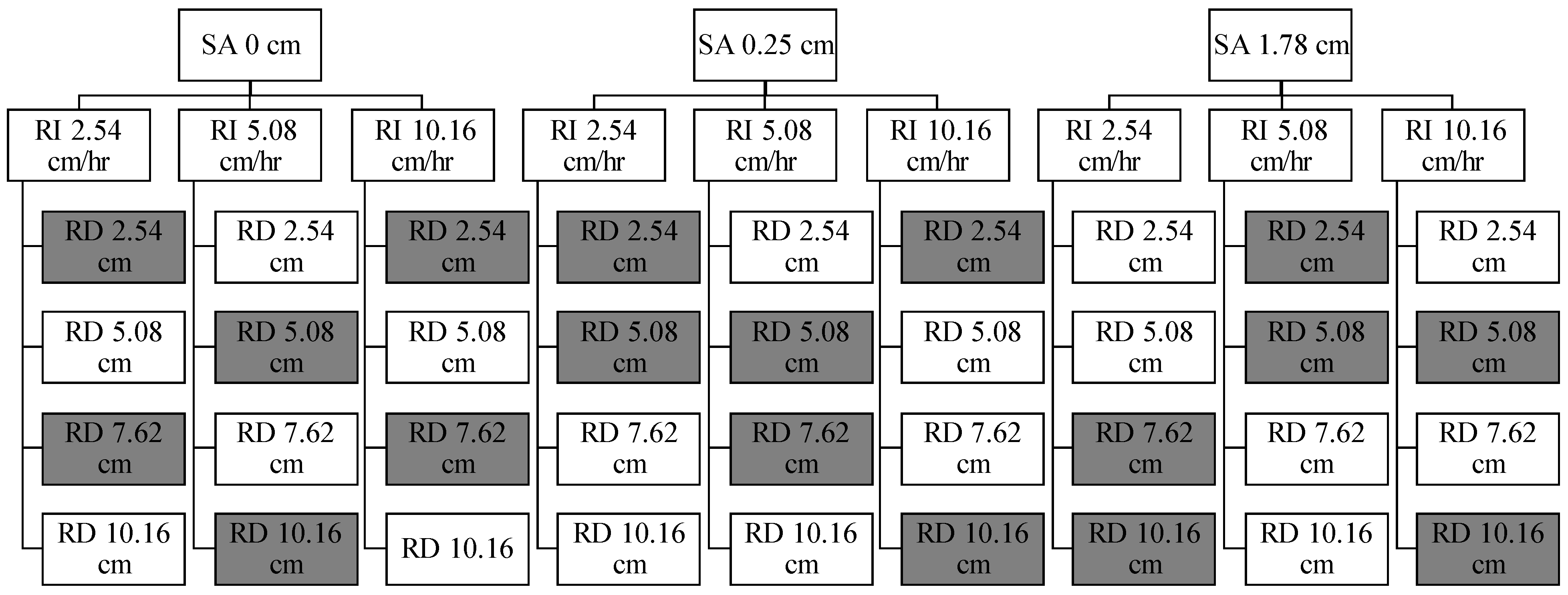
The modelled RDs were 2.54, 5.08, 7.67, and 10.16 cm (1, 2, 3, 4 inches, repectively), which are based on 88–99 percentile of rainfalls that were measured during last 10 years at Belleville in the State of Illinois. Based on Southwest Illinois IDF table, RIs of 2.54, 5.08, and 10.16 cm/h (1, 2, 4 inch/h, repectively) were used in the modeling. The modelled SA (i.e., sediment build-ups) were 0, 0.25, and 1.78 cm (or TT 0, 0.3, and 5.6 min., respectively), which represent the thickeness of the sediment layers on the surface of the bioswales. A total of 72 scenarios were simulated, which include 36 scenarios for each of AR at 9% and 13%. These 36 scenarios are identical except AR and are illustrated in Figure 5. Results from half of the simulated scenarios (i.e., the shaded scenarios in Figure 5 for each AR) were used to develop the mathematical model. Results from the other half of simulated scenarios (i.e., those not shaded in Figure 5 for each AR) were used to validate the developed mathematical model. Further information of these simulated scenarios is summarized in Table 3.
5. Simulation Results of Runoffs from the Idealized Catchment Area
Results of the 72 simulated scenarios on stormwater runoffs are illustrated in Figure 6, Figure 7 and Figure 8. The runoffs are from the bioswales that capture the stormwater runoffs from the idealized catchment areas shown in Figure 4.
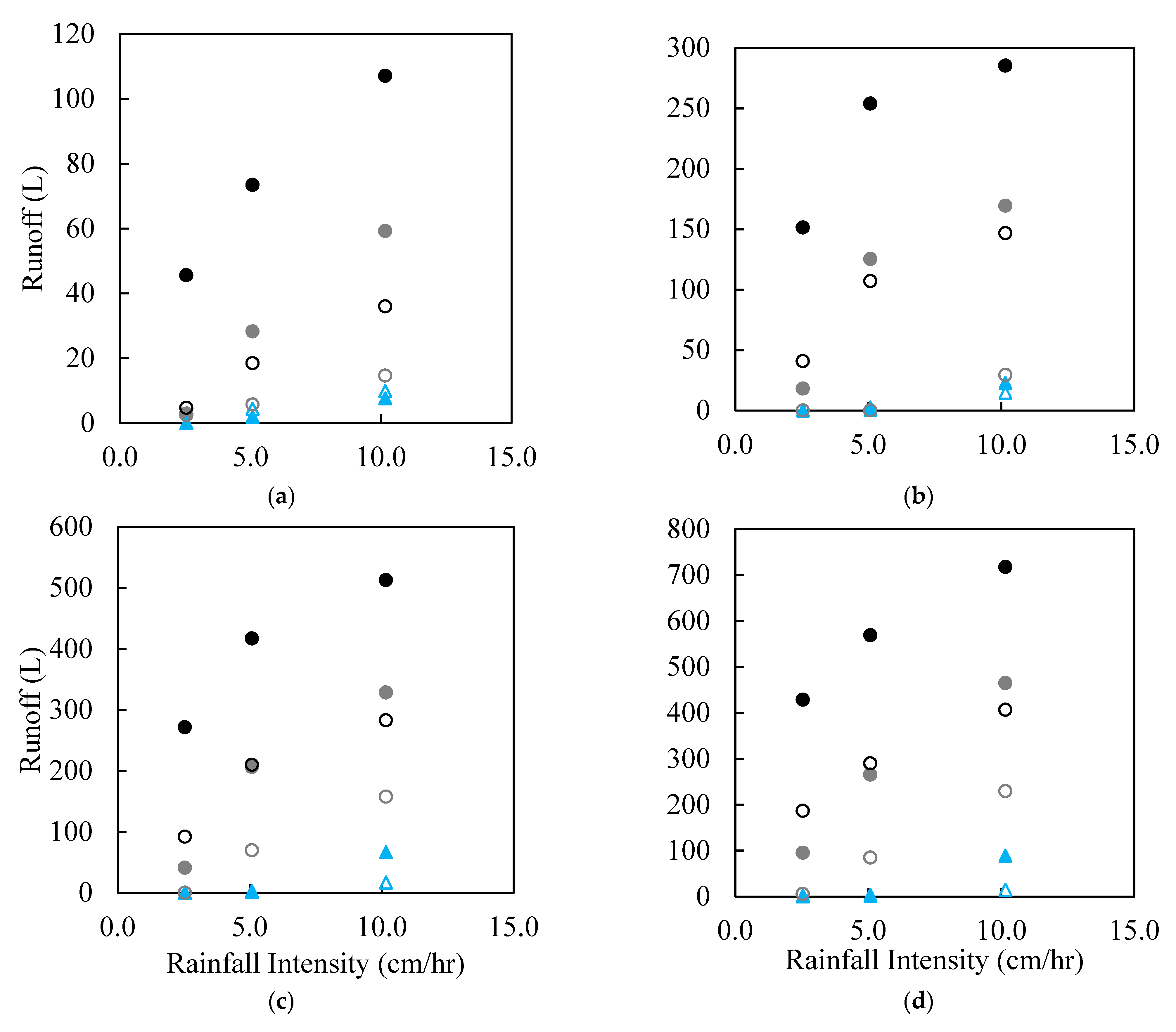
Figure 6 illustrates the effect of RD on the runoffs from the bioswales under the impact of three SA and two AR conditions. Each sub-figure of Figure 6 illustrates one of four simulated RDs. Figure 6 reveals that the positive correlations between runoffs from the bioswales and RI and AR are best described by a polynomial equation, instead of a linear equation. The incremental increase of bioswale runoffs becomes increasingly prominent at higher RI and increased RD.
As indicated in Figure 6, when there is no sediment build-up (i.e., TT 0 min), a change of AR from 9% to 13% did not result in a noticeable difference in runoffs from the bioswale. At RIs of 5.08 cm/h or lower, bioswale runoffs were affected predominantly by the soil’s infiltration rate and the amount of stormwater run-ons to the bioswale. When the bioswale are covered with sediment build-ups (i.e., TT 0.3 and 5.6 min), under conditions of larger rainfalls (i.e., RI of 5.08 cm/h or higher, RD of 7.62 cm or higher), AR has a large impact on bioswale runoffs: the runoff at AR 9% was more than twice of the runoff at AR 13%, because the unit surface area of the bioswale at AR 9% received 44.4% more stormwater runoffs than that at AR 13%. The soil infiltration rate limits the rate of draining the stormwater run-ons into the bioswale under the conditions of large rainfalls, resulting in larger stormwater runoffs from the bioswales as revealed from the simulations results. At conditions of low rainfall (i.e., RI of lower than 5.08 cm/h, RD of lower than 7.62 cm), the difference in bioswale runoffs between AR 9% and AR 13% was negligible, indicating soil infiltration rate was adequate to rapidly drain the stormwater run-ons to bioswale that occurred at these low rainfall conditions.
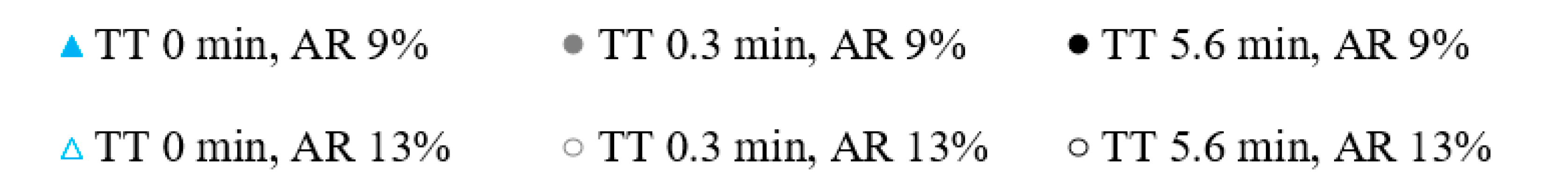
Results shown in Figure 7 indicated that when there is no sediment build-up (i.e., TT 0 min), the amount of bioswale runoffs was insignificant. At the highest simulated RI of 10.16 cm/h, the runoff was approximately only 8.5% (i.e., 80 L) of the 942 L run-on to the bioswale; and there was no significant difference in bioswale runoffs between AR 9% and AR 13%. However, bioswale runoffs increase substantially when there are sediment build-ups on the surface of the bioswales (i.e., TT 0.3 min or 5.6 min). The increase of runoffs appears to fit a power-law relationship between bioswale runoffs and simulated TTs.
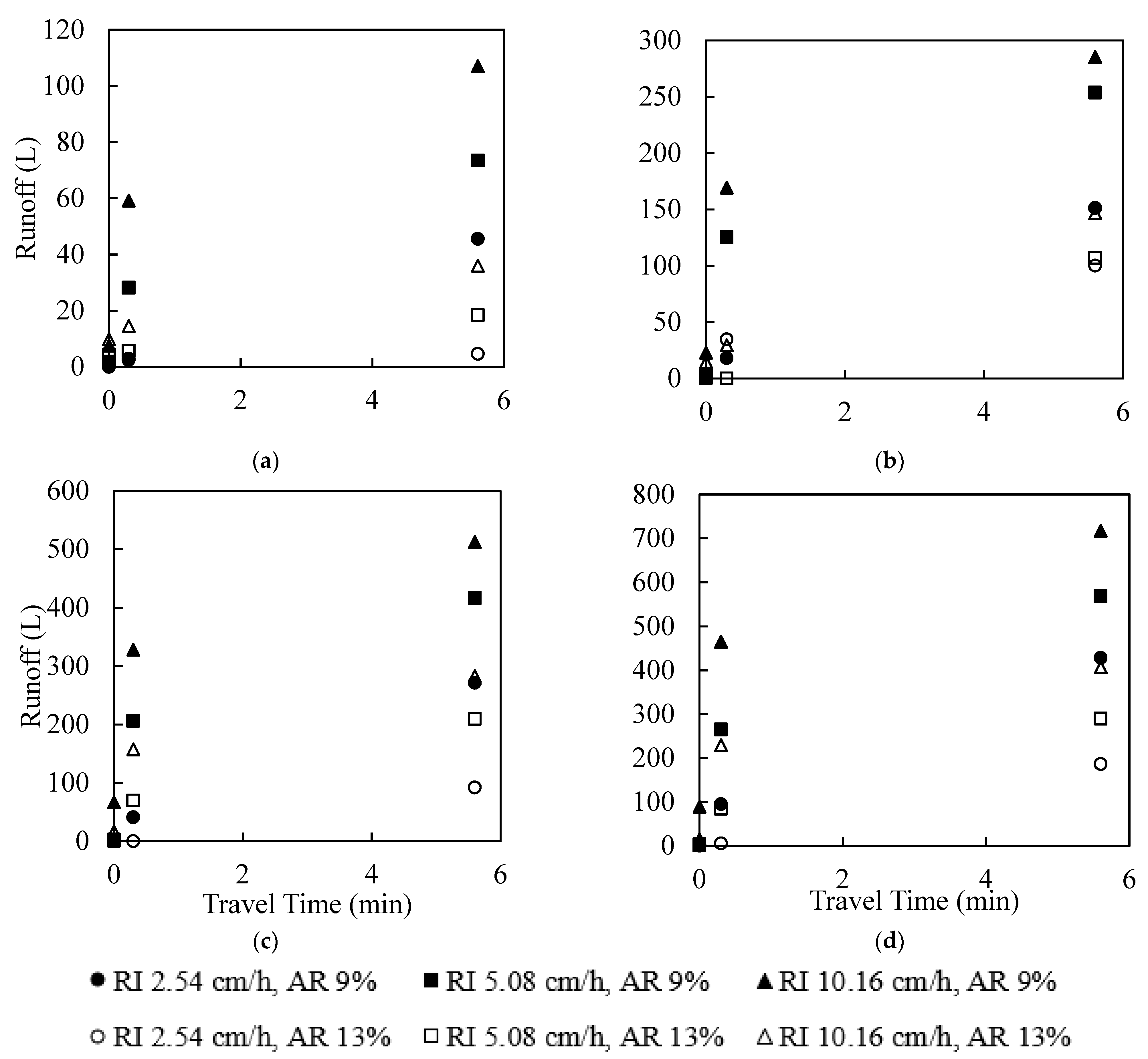
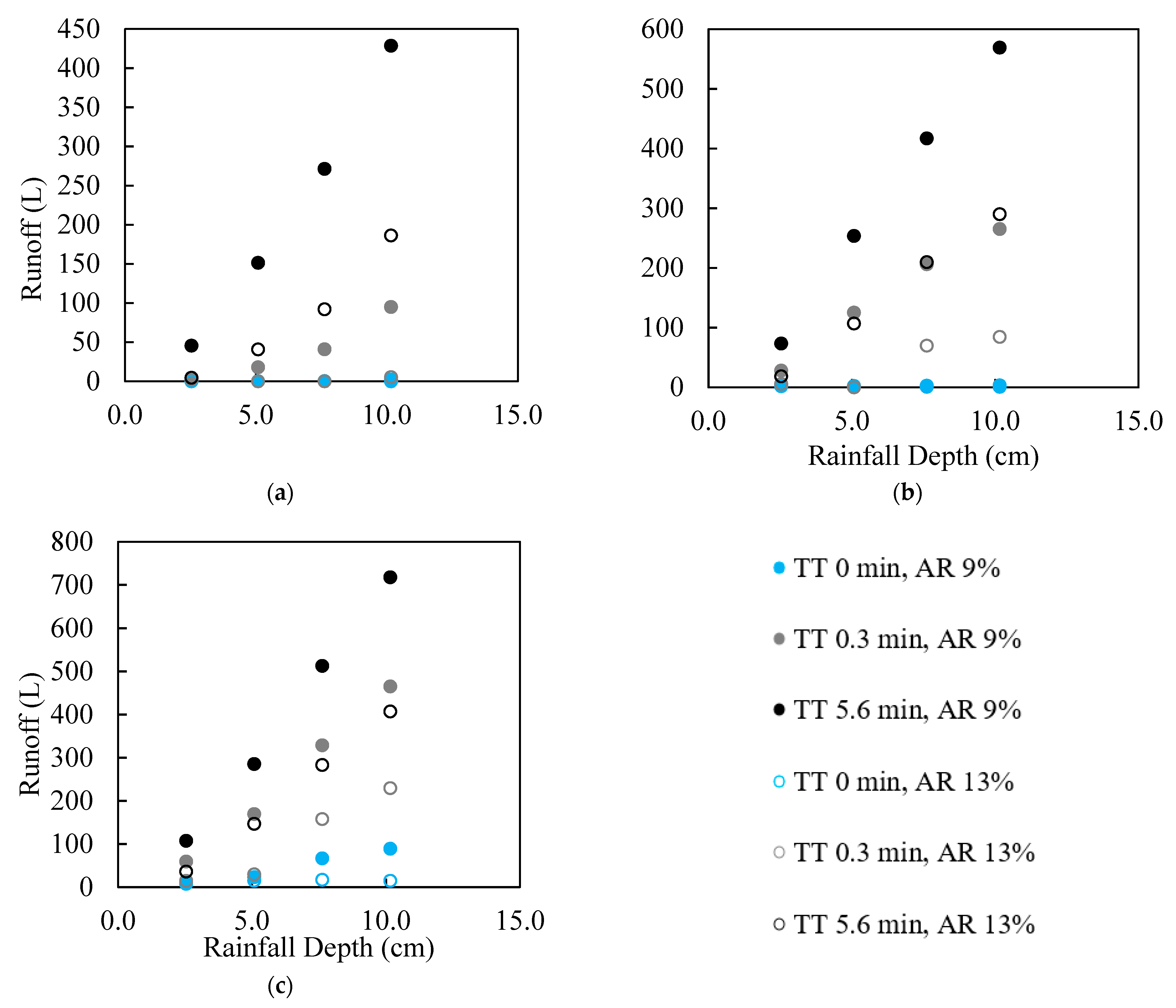
The effect of the RD on bioswale runoffs are shown in Figure 8. Higher RI or RD resulted in increased runoffs. Apparently, RD has a larger impact than RI on the runoff. As an example, at AR 9% and TT of 5.6 min., when the RD increased from 2.54 cm to 10.16 cm, at the RI of 2.54 cm/h, the runoffs increased from 50 L to 425 L (Figure 8a); while at RI of 10.16 cm/h, the runoffs increased from 125 L to 710 L (Figure 8c). The correlation between runoff and RD appears to follow a second-degree polynomial relationship.
6. Developing a Simplified Mathematical Model for Runoff Prediction
Among the 72 studied scenarios, PCSWMM simulation results of 36 scenarios that were randomly selected (columns 1–5 of Table 3) were used to develop a preliminary mathematical model; PCSWMM simulation results of the remaining 36 scenarios (columns 6–10 of Table 3) were used to optimize and validate the model. Four parameters (AR, RD, RI, TT) that are most influential on bioswale runoffs were included in the simplified mathematical model.
To develop the mathematical model, MATLAB curve-fitting command was used to develop the most fitting mathematical relationship. Results from PCSWMM simulation were used as input values of the MATLAB curve-fitting program to generate the runoff equation and coefficients for each of four parameters. The MATLAB program minimizes the difference between the PCSWMM-simulated runoffs and the mathematically-calculated runoffs.
The developed mathematical equation was optimized further by comparing PCSWMM runoffs of the second set of 36 scenarios with mathematical model-calculated runoffs. When major differences were found, the coefficients of the equations were adjusted until difference was minimized and reached a highest possible R-squared value. The R-squared value of the Equation (2) is 0.967. The developed mathematical models are shown in Equations (2)–(6):
where,
: Runoff (L),
: Area Ratio (%),
: Traveling Time (min),
: Rainfall Depth (,
: Rainfall Intensity (cm/h),
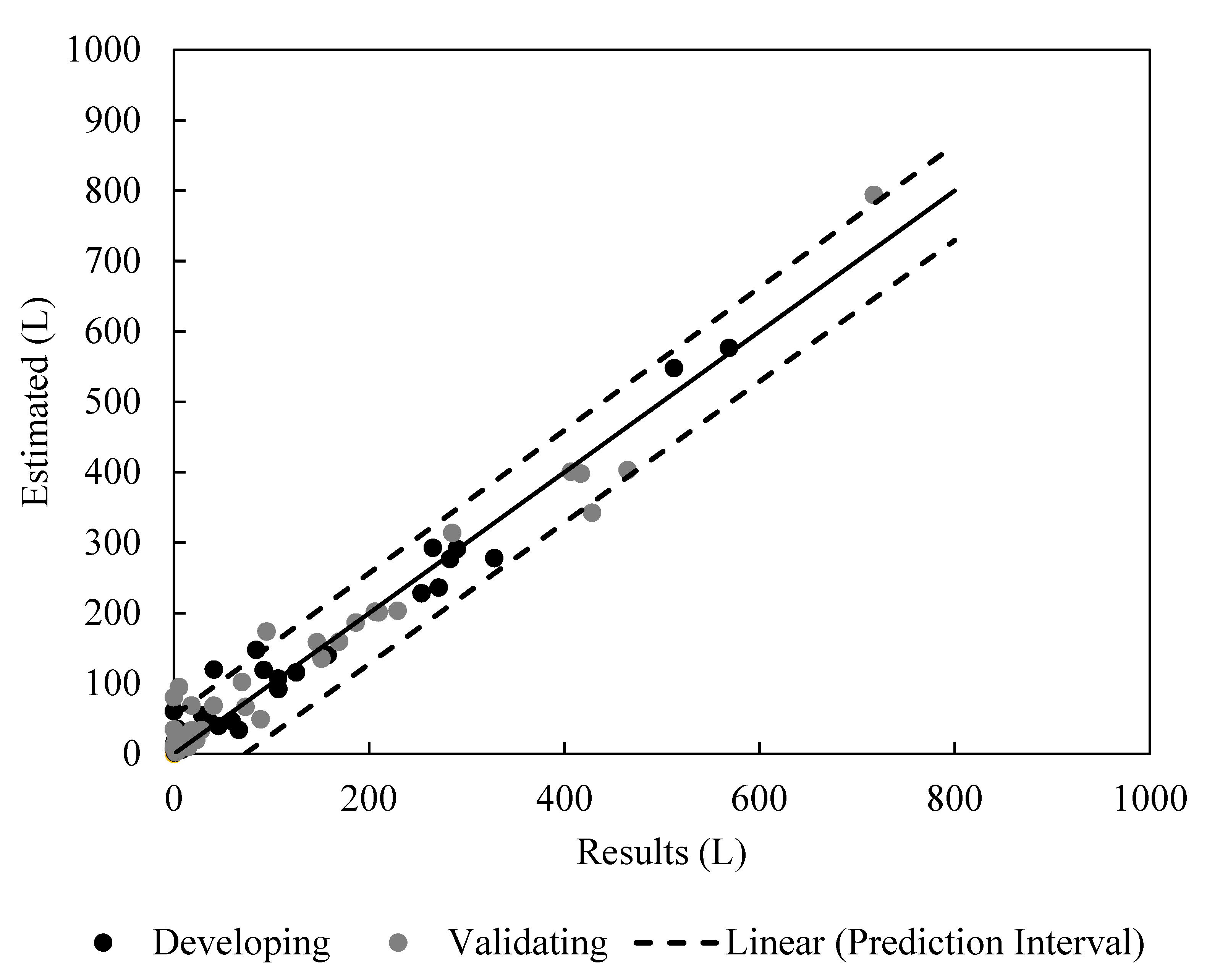
The comparisons between the runoffs calculated by the newly developed mathematical equation and the runoffs simulated by PCSWMM are illustrated in Figure 9. The first and second set of 36 scenarios which were used for model development and testing are shown in black and gray symbols, respectively. The solid line shows the line of 1:1 agreement between math equation-predicted runoffs and PCSWMM-simulated runoffs. The two dashed lines show the 95% confidence intervals of the mathematical equation. The Mean Absolute Percentage Error (MAPE) between the calculated runoffs using the mathematical equation and the simulated runoffs with PCSWMM of the 72 scenarios is less than 18%, which shows a reasonable estimate of the mathematical model.
The applicable range of the equation based on the finding in this study is presented in Table 4. It is noted that the soil condition was set as clay in PCSWMM modeling of the idealized catchment areas. Because clay’s water infiltration rate is the lowest among commonly encountered other types of soils, the calculated runoffs using Equation (2) will predict the maximum amount of runoff from a given site.
7. Engineering Application of the New Mathematical Model
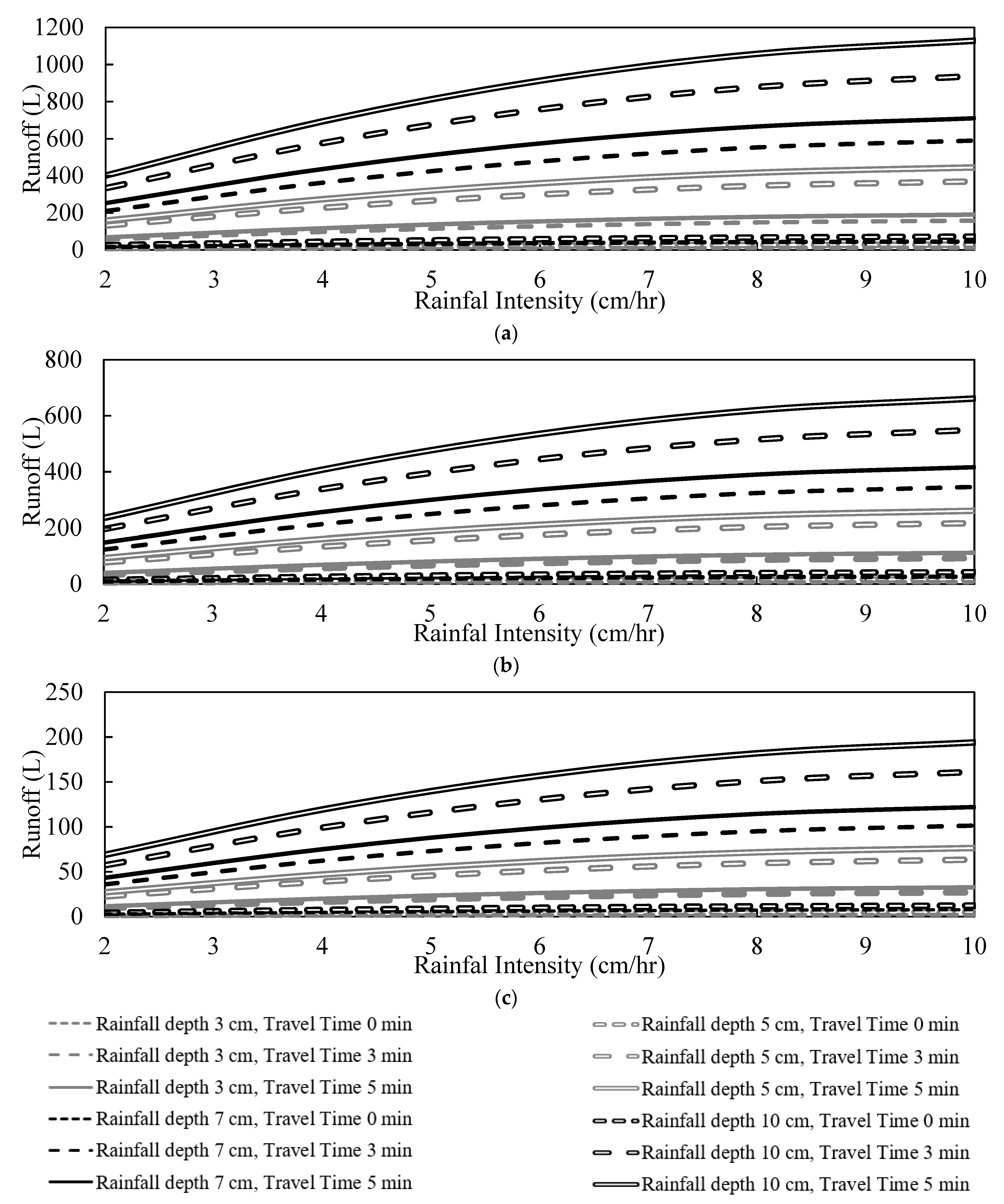
It is important to predict bioswale’s abilities to reduce stormwater runoffs from roadways. Although SWMM is a valuable tool that can simulate project-specific conditions in support of engineering designs, the complexity and required special modeling skills make it difficult to conduct routine SWMM modeling and simulations. A simple mathematical equation can provide a reliable and easy-to-use tool for predicting a bioswale’s performance. For this purpose, a set of nomographs, developed by using the newly developed mathematical equations, are illustrated in Figure 10. Engineering designers and stormwater managers can use these nomographs to predict stormwater runoffs based on the conditions of their key design parameters (AR, RD, RI, SA). The graphs can be used to calculate the runoff produced from linear bioswales along highways subjected to RI of 2 to 10 cm/h, RD of 3 to 10 cm, and traveling time (TT) of 0 to 5 min. The TT of 0 represents new bioswales. The TT of 5 min represents represent 1.78 cm-thick layer of sediments with permeability of 150 cm/h that were accumulated during 10 years with 0.19 kg/m2/year sediment accumulation rates.
The limitations of this newly developed mathematical model in its current form are recognized. The coefficients in Equations (3)–(6) are affected by specific conditions of key parameters that were used for developing the mathematical model, such as Southwest Illinois-based rainfall data, turf type of vegetation cover for unpaved areas, clay soils, sediment accumulation rate and pattern, the geometric layout of the idealized catchment model, and the design of the bioswale including the area ratio. However, the methodology presented by this study can be used to develop applicable mathematical equations and nomographs from a range of conditions such as different rainfall patterns across the country and various types of surface vegetation cover and soil. An atlas can be developed from such expanded work, which can provide a valuable tool to stormwater and environmental professionals and the engineering community.
8. Summary and Conclusions
This study investigated the effects of area ratio, rainfall depth, rainfall intensity, and sediment accumulation on stormwater runoff reduction by bioswales. PCSWMM was used to simulate various scenarios of these parameters. The PCSWMM model was validated with measured results of field testing.
Findings from this study indicate that higher sediment accumulation resulted in increased runoff from the bioswale. Such an effect was intensified when the effects of rainfall depth and rainfall intensity were incorporated in the analysis. At area ratios of 9% and 13%, the runoffs were comparable and were nearly zero under rainfalls of less than 5 cm/h with the travel time of 0 min (i.e., no sediment accumulation). However, increases in travel time to 0.3 and 5.6 min resulted in increase in runoffs at area ratios of both 9% and 13% under rainfalls of more than 5 cm/h. The runoff from area ratio of 9% was more than twice of the runoff from area ratio of 13%. Furthermore, under a rainfall intensity of 2.54 cm/h, area ratio of 9%, and travel time of 5 min (i.e., sediment accumulation of 1.78 cm), a rainfall depth of 10.16 cm resulted in a runoff of 8.5 times the runoff from a rainfall depth of 2.54 cm.
This study has developed a simplified mathematical model for predicting the effectiveness of a bioswale’s control on stormwater runoff from roadways and a set of associated nomographs that engineering designers and stormwater managers can use to predict stormwater runoffs based on the conditions of their key design parameters. Such a simplified model can help to alleviate the difficulties of securing specialized technical expertise for handling sophisticated modeling tools. It is recommended that the work presented in this study be expanded to address a broad range of hydrologic and site conditions to benefit wide application of this newly developed model for use by stormwater and environmental professionals and the engineering community.
Author Contributions
Conceptualization, A.O., J.Z.; methodology, A.O., J.Z., A.A.B., S.N.; software, A.A.B., S.N.; validation, A.O., J.Z., A.A.B., S.N.; formal analysis, S.N.; investigation, A.O., J.Z, A.A.B., S.N.; data curation, A.A.B., S.N.; writing—original draft preparation, J.Z; writing—review and editing, J.Z., A.O.; visualization, S.N.; supervision, A.O., J.Z.; project administration, A.O.; funding acquisition, A.O., J.Z. All authors have read and agreed to the published version of the manuscript.
Funding
This research was funded by ICT/IDOT ICT R27-141, grant number 2011-05776-30. This publication reports the expanded work by the authors from their work of ICT R27-141 Effective Post-Construction Best Management Practices to Infiltrate and Retain Stormwater Run-off. ICT R27-141 was conducted in cooperation with the Illinois Center for Transportation, the Illinois Department of Transportation (IDOT) Office of Program Development, and the US Department of Transportation Federal Highway Administration. The authors would like to acknowledge the members of IDOT Technical Review Panel (TRP) for their valuable advice at different stages of this research, and Southern Illinois University Edwardsville for the academic resources that supported this study. The contents of this paper reflect only the views of the authors.
Institutional Review Board Statement
Not applicable.
Informed Consent Statement
Not applicable.
Data Availability Statement
Data, models, or code generated for this study, including field tests results and modeling input files are available from the corresponding author by request.
Conflicts of Interest
The authors declare no conflict of interest.
References
- AASHTO. A Policy All Design Standards Interstate System; Standing Committee on Highways AASHTO Highway Subcommittee on Design Technical Committee on Geometric Design: Washington, DC, USA, 2005. [Google Scholar]
- Ackerman, D.; Stein, E.D. Evaluating the Effectiveness of Best Management Practices Using Dynamic Modeling. J. Environ. Eng. 2008, 134, 628–639. [Google Scholar] [CrossRef]
- Akhavan Bloorchian, A. Effect of Major Factors on Bioswale Performance and Hydrologic Processes for the Control of Stormwater Runoff from Highways. Ph.D. Thesis, Southern Illinois University, Carbondale, IL, USA, 2018. [Google Scholar]
- Beyerlein, D. Low Impact Development Computations—WWHM. In World Environmental and Water Resources Congress 2011: Bearing Knowledge for Sustainability; ASCE: Restone, VA, USA, 2011; pp. 558–576. [Google Scholar]
- Caltrans. BMP Retrofit Pilot Program Final Report; CTSW-RT 01-050; California Department of Transportation: Sacramento, CA, USA, 2004.
- Chen, W. Monitoring and Modeling of the Hydrologic Performance of the Carroll Street Right-of-Way Bioswale. Master’s Thesis, Department of Civil, Architectural, and Environmental Engineering, Drexel University, Philadelphia, PA, USA, 2014. [Google Scholar]
- Clary, J.; Leisenring, M.; Quigley, M.; Jones, J.; Strecker, E. International Stormwater Best Management Practices (BMP) Database, Narrative Overview of BMP Database Study Characteristics; Wright Water Engineers, Inc. Geosyntec Consultant: Water Environment Research Foundation: Alexaandra, VA, USA, 2012. [Google Scholar]
- Geosyntec. Post-Construction BMP Technical Guidance Manual; Storm Water BMP Guidance Manual: Santa Barbara, CA, USA, 2008.
- Geosyntec and Wright Water Inc. International Stormwater Best Management Practices (BMP) Database Individual BMP Summaries: Chesapeake Bay and Related Areas; The Water Research Doundation: Alexandra, VA, USA, 2012. [Google Scholar]
- Harwood, D.W.; Hutton, J.M.; Fees, C.; Bauer, K.M.; Glen, A.; Ouren, H. Evaluation of the 13 Controlling Criteria for Geometric Design; NCHRP 783 (No. Project 17-53); The National Academies Press: Washington, DC, USA, 2014. [Google Scholar]
- Huber, W.C. Use of EPA SWMM5 for Generation of BMP Effluent EMC Distribution. In Proceedings of the Second BMP Technology Symposium, EWRI World Water and Environmental Resources Congress, Omaha, Nebraska, 21–25 May 2006. [Google Scholar]
- Heaney, J.P.; Sample, D.; Wright, L.; Fan, C. Costs of Urban Stormwater Control; US Environmental Protection Agency, Office of Research and Development, National Risk Management Research Laboratory: Cincinnati, OH, USA, 2002.
- Illinois Department of Transportation (IDOT). Drainage Manual; Illinois Department of Transporation: Springfield, IL, USA, 2011.
- Illinois Environmental Protection Agency (IEPA, 2013). Stormwater Performance Standards Recommendations; Post-Development Stormwater Runoff Standards (PDSWRS); Workgroup and Association of Illinois Soil and Water Conservation Districts (AISWCD): Springfield, IL, USA, 2013.
- James, W.; Rossman, L.E.; James, W.R. User’s Guide to SWMM 5, 13th ed.; CHI Press Publication: Guelph, ON, Canada, 2010. [Google Scholar]
- Li, H. Green infrastructure for Highway Stormwater Management: Field Investigation for Future Design, Maintenance, and Management Needs. J. Infrastruct. Syst. 2015, 21, 05015001. [Google Scholar] [CrossRef]
- Li, J.; Orland, R.; Hogenbirk, T. Environmental Road and Lot Drainage Designs: Alternatives to Curb-Gutter-Sewer System. Can. J. Civ. Eng. 1998, 25, 26–39. [Google Scholar] [CrossRef]
- NCHRP. Evaluation of Best Management Practices for Highway Runoff Control; Report 565; Transportation Research Board: Washington, DC, USA, 2006. [Google Scholar]
- NCHRP. Guidelines for Evaluating and Selecting Modifications to Existing Roadway Drainage Infrastructure to Improve Water Quality in Ultra-Urban Areas; Report 728; Transportation Research Board: Washington, DC, USA, 2012. [Google Scholar]
- NCHRP. Long-Term Performance and Life-Cycle Costs of Stormwater Best Management Practices; Report 792; Transportation Research Board: Washington, DC, USA, 2014. [Google Scholar]
- Natural Resources Conservation Service (NRCS). Technical Guide, Section I, Erosion Prediction; NRCS: Champaign, IL, USA, 1997. Available online: https://efotg.sc.egov.usda.gov/references/public/IL/ArchivedRUSLE.pdf (accessed on 13 December 2017).
- Osouli, A.; Bloorchian, A.A.; Grinter, M.; Alborzi, A.; Marlow, S.L.; Ahiablame, L.; Zhou, J. Performance and Cost Perspective in Selecting BMPs for Linear Projects. Water 2017, 9, 302. [Google Scholar] [CrossRef] [Green Version]
- Osouli, A.; Bloorchian, A.A.; Nassiri, S.; Marlow, S.L. Effect of Sediment Accumulation on Best Management Practice (BMP) Stormwater Runoff Volume Reduction Performance for Roadways. Water 2017, 9, 980. [Google Scholar] [CrossRef] [Green Version]
- Osouli, A.; Grinter, M.; Zhou, J.; Ahiablame, L.; Stark, T. Effective Post-Construction Best Management Practices (BMPs) to Infiltrate and Retain Stormwater Run-Off; Report No. FHWA-ICT-17-011; Illinois Center for Transportation/Illinois Department of Transportation: Rantoul, IL, USA, 2017. [Google Scholar]
- Pellant, M.; Shaver, P.; Pyke, D.A.; Herrick, J.E. Interpreting Indicators of Rangeland Health, Version 4. Technical Reference 1734-6; BLM/WO/ST-00/001+1734/REV05; U.S. Department of the Interior, Bureau of Land Management, National Science and Technology Center: Denver, CO, USA, 2005; p. 122.
- Poresky, A.; Bracken, C.; Strecker, E.; Clary, J. International Stormwater Best Management Practices (BMP) Database, Technical Summary: Volume Reduction; Geosyntec Consultants & Wright Water Engineers, Inc. Water Environment Research Foundation: Alexaandra, VA, USA, 2011. [Google Scholar]
- Roess, R.P.; Prasses, E.S.; McShane, W.R. Traffic Engineering, 4th ed.; Prentice Hall: Hoboken, NJ, USA, 2011; ISBN 978-0136135739. [Google Scholar]
- Stevens, M.R. Assessment of Water Quality, Road Runoff, and Bulk Atmospheric Deposition, Guanella Pass Area, Clear Creek and Park Counties, Colorado, Water Years 1995–97; US Department of the Interior, US Geological Survey: Washington, DC, USA, 2001.
- Strecker, E.; Poresky, A.; Roseen, R.; Soule, J.; Gummadi, V.; Dwivedi, R.; Littleton, C.O. Volume Reduction of Highway Runoff in Urban Areas: National Cooperative Highway Research Program (NCHRP) Report 802; Transportation Research Board (TRB): Washington, DC, USA, 2015. [Google Scholar]
- Sun, Y.W.; Li, Q.Y.; Liu, L.; Xu, C.D.; Liu, Z.P. Hydrological simulation approaches for BMPs and LID practices in highly urbanized area and development of hydrological performance indicator system. Water Sci. Eng. 2014, 7, 143–154. [Google Scholar]
- Urban Drainage and Flood Control District (UDFCD). Urban Strom Drainage-Criteria Manual—Volume 1: Management, Hydrology, and Hydraulics; Urban Drainage and Flood Control District: Denver, CO, USA, 2008.
- Xiao, Q.; McPherson, G.E. Testing a Bioswale to Treat and Reduce Parking Lot Runoff; University of California, Davis and USDA Forest Service: Washington, DC, USA, 2009. [Google Scholar]
Figure 1.
Field-tested Bioswale Unit: (a) Plan View; (b) Section View (modified after [23]).
Figure 1.
Field-tested Bioswale Unit: (a) Plan View; (b) Section View (modified after [23]).

Figure 2.
PCSWMM Modelled Field-Tested Bioswale Unit (a) Plan view; (b) Section view [23].
Figure 2.
PCSWMM Modelled Field-Tested Bioswale Unit (a) Plan view; (b) Section view [23].

Figure 3.
Validation of PCSWMM model (simulated vs. field-measured).

Figure 4.
Idealized (conceptual) catchment model for highways.

Figure 5.
Simulated scenarios for developing a simplified mathematical model. SA = Sediment Accumulation (i.e., Build-up), RI = Rainfall Intensity, RD = Rainfall Depth.
Figure 5.
Simulated scenarios for developing a simplified mathematical model. SA = Sediment Accumulation (i.e., Build-up), RI = Rainfall Intensity, RD = Rainfall Depth.

Figure 6.
Effect of RI on runoffs from bioswales, under various TT and AR conditions at RD of (a) 2.54 cm, (b) 5.08 cm, (c) 7.62 cm, (d) 10.16 cm.
Figure 6.
Effect of RI on runoffs from bioswales, under various TT and AR conditions at RD of (a) 2.54 cm, (b) 5.08 cm, (c) 7.62 cm, (d) 10.16 cm.


Figure 7.
Effect of sediment build-up (travel time) on runoffs from bioswales, under RI and AR conditions at RD of (a) 2.54 cm, (b) 5.08 cm, (c) 7.62 cm, (d) 10.16 cm.
Figure 7.
Effect of sediment build-up (travel time) on runoffs from bioswales, under RI and AR conditions at RD of (a) 2.54 cm, (b) 5.08 cm, (c) 7.62 cm, (d) 10.16 cm.

Figure 8.
Effect of rainfall depth on runoffs from bioswales, under various TT and AR conditions at rainfall intensity of (a) 2.54 cm/h, (b) 5.08 cm/h, (c) 10.16 cm/h.
Figure 8.
Effect of rainfall depth on runoffs from bioswales, under various TT and AR conditions at rainfall intensity of (a) 2.54 cm/h, (b) 5.08 cm/h, (c) 10.16 cm/h.

Figure 9.
Correlation between new mathematical model calculated runoffs with PCSWMM-simulated runoffs.
Figure 9.
Correlation between new mathematical model calculated runoffs with PCSWMM-simulated runoffs.

Figure 10.
Nomographs for Predicting Bioswale Runoffs (a) AR 5%, (b) AR 10%, (c) AR 15%.


Table 1.
Material description (LL = Liquid Limit, PL = Plastic Limit).
| Material | Infiltration Rate (cm/min) | Specific Gravity | Void Ratio | Bulk Density (kg/m3) | LL (%) | PL (%) | Soil Description |
|---|---|---|---|---|---|---|---|
| Natural Soil | 0.5 | 2.65 | 0.56 | 1723 | 30 | 20 | Sandy Lean Clay |
| Growing Medium | - | - | 0.45 | - | 0 | 0 | Highly Organic |
| Aggregate | - | 2.63 | 0.42 | - | 0 | 0 | Crushed Gravel |
Table 2.
Rainfalls for Bioswale Field Testing.
| Rainfalls | Volume (L) | Duration (Min) | Intensity (cm/h) |
|---|---|---|---|
| 10-year-return | 945 | 10 | 15.24 |
| 2-year-return | 945 | 20 | 7.62 |
| 9-month-return | 945 | 45 | 3.39 |
Table 3.
Developing and optimizing a simplified mathematical model.
| 36 Scenarios for Developing the Model | ||||
|---|---|---|---|---|
| AR | RD | RI | TT | Runoff |
| (%) | (cm) | (cm/h) | (min) | (L) |
| 9 | 2.54 | 2.54 | 0 | 2.05 |
| 9 | 2.54 | 10.16 | 0 | 7.57 |
| 9 | 5.08 | 5.08 | 0 | 12.43 |
| 9 | 7.62 | 2.54 | 0 | 14.42 |
| 9 | 7.62 | 10.16 | 0 | 36.66 |
| 9 | 10.16 | 5.08 | 0 | 31.42 |
| 9 | 2.54 | 2.54 | 0.3 | 12.88 |
| 9 | 2.54 | 10.16 | 0.3 | 59.20 |
| 9 | 5.08 | 5.08 | 0.3 | 125.30 |
| 9 | 7.62 | 2.54 | 0.3 | 40.98 |
| 9 | 7.62 | 10.16 | 0.3 | 328.40 |
| 9 | 10.16 | 5.08 | 0.3 | 265.30 |
| 9 | 2.54 | 2.54 | 5.6 | 45.56 |
| 9 | 2.54 | 10.16 | 5.6 | 107.05 |
| 9 | 5.08 | 5.08 | 5.6 | 253.70 |
| 9 | 7.62 | 2.54 | 5.6 | 271.39 |
| 9 | 7.62 | 10.16 | 5.6 | 512.61 |
| 9 | 10.16 | 5.08 | 5.6 | 568.95 |
| 13 | 2.54 | 2.54 | 0 | 1.38 |
| 13 | 2.54 | 10.16 | 0 | 2.84 |
| 13 | 5.08 | 4.572 | 0 | 5.40 |
| 13 | 7.62 | 2.54 | 0 | 1.24 |
| 13 | 7.62 | 10.16 | 0 | 16.78 |
| 13 | 10.16 | 5.08 | 0 | 9.96 |
| 13 | 2.54 | 2.54 | 0.3 | 0.00 |
| 13 | 2.54 | 10.16 | 0.3 | 14.57 |
| 13 | 5.08 | 4.572 | 0.3 | 29.48 |
| 13 | 7.62 | 2.54 | 0.3 | 32.74 |
| 13 | 7.62 | 10.16 | 0.3 | 157.53 |
| 13 | 10.16 | 5.08 | 0.3 | 84.50 |
| 13 | 2.54 | 2.54 | 5.6 | 4.63 |
| 13 | 2.54 | 10.16 | 5.6 | 35.96 |
| 13 | 5.08 | 4.572 | 5.6 | 107.00 |
| 13 | 7.62 | 2.54 | 5.6 | 92.05 |
| 13 | 7.62 | 10.16 | 5.6 | 282.95 |
| 13 | 10.16 | 5.08 | 5.6 | 289.92 |
| 9 | 2.54 | 5.08 | 0 | 1.89 |
| 9 | 5.08 | 2.54 | 0 | 8.20 |
| 9 | 5.08 | 10.16 | 0 | 22.93 |
| 9 | 7.62 | 5.08 | 0 | 22.84 |
| 9 | 10.16 | 2.54 | 0 | 12.35 |
| 9 | 10.16 | 10.16 | 0 | 48.89 |
| 9 | 2.54 | 5.08 | 0.3 | 28.20 |
| 9 | 5.08 | 2.54 | 0.3 | 18.10 |
| 9 | 5.08 | 10.16 | 0.3 | 169.35 |
| 9 | 7.62 | 5.08 | 0.3 | 206.26 |
| 9 | 10.16 | 2.54 | 0.3 | 95.05 |
| 9 | 10.16 | 10.16 | 0.3 | 464.91 |
| 9 | 2.54 | 5.08 | 5.6 | 73.44 |
| 9 | 5.08 | 2.54 | 5.6 | 151.38 |
| 9 | 5.08 | 10.16 | 5.6 | 285.20 |
| 9 | 7.62 | 5.08 | 5.6 | 417.03 |
| 9 | 10.16 | 2.54 | 5.6 | 428.55 |
| 9 | 10.16 | 10.16 | 5.6 | 717.30 |
| 13 | 2.54 | 5.08 | 0 | 1.39 |
| 13 | 5.08 | 2.54 | 0 | 3.22 |
| 13 | 5.08 | 10.16 | 0 | 14.78 |
| 13 | 7.62 | 5.08 | 0 | 0.87 |
| 13 | 10.16 | 2.794 | 0 | 5.06 |
| 13 | 10.16 | 10.16 | 0 | 14.52 |
| 13 | 2.54 | 5.08 | 0.3 | 5.68 |
| 13 | 5.08 | 2.54 | 0.3 | 0.00 |
| 13 | 5.08 | 10.16 | 0.3 | 21.03 |
| 13 | 7.62 | 5.08 | 0.3 | 69.78 |
| 13 | 10.16 | 2.794 | 0.3 | 85.31 |
| 13 | 10.16 | 10.16 | 0.3 | 229.24 |
| 13 | 2.54 | 5.08 | 5.6 | 18.43 |
| 13 | 5.08 | 2.54 | 5.6 | 40.85 |
| 13 | 5.08 | 10.16 | 5.6 | 146.61 |
| 13 | 7.62 | 5.08 | 5.6 | 209.80 |
| 13 | 10.16 | 2.794 | 5.6 | 186.35 |
| 13 | 10.16 | 10.16 | 5.6 | 406.76 |
Table 4.
Suitable range of parameters by the new mathematical equation.
| Area Ratio (AR) | Traveling Time (TT) | Rainfall Depth (RD) | Rainfall Intensity (RI) |
|---|---|---|---|
| (%) | (Min) | (cm) | (cm/h) |
| Up to 17 | Up to time of concentration | Greater than 1.45 | Up to 21.9 |
Publisher’s Note: MDPI stays neutral with regard to jurisdictional claims in published maps and institutional affiliations. |
© 2021 by the authors. Licensee MDPI, Basel, Switzerland. This article is an open access article distributed under the terms and conditions of the Creative Commons Attribution (CC BY) license (https://creativecommons.org/licenses/by/4.0/).
Share and Cite
MDPI and ACS Style
Zhou, J.; Bloorchian, A.A.; Nassiri, S.; Osouli, A. A Simplified Model for Predicting the Effectiveness of Bioswale’s Control on Stormwater Runoff from Roadways. Water 2021, 13, 2798. https://doi.org/10.3390/w13202798
AMA Style
Zhou J, Bloorchian AA, Nassiri S, Osouli A. A Simplified Model for Predicting the Effectiveness of Bioswale’s Control on Stormwater Runoff from Roadways. Water. 2021; 13(20):2798. https://doi.org/10.3390/w13202798
Chicago/Turabian StyleZhou, Jianpeng, Azadeh Akhavan Bloorchian, Sina Nassiri, and Abdolreza Osouli. 2021. "A Simplified Model for Predicting the Effectiveness of Bioswale’s Control on Stormwater Runoff from Roadways" Water 13, no. 20: 2798. https://doi.org/10.3390/w13202798
Note that from the first issue of 2016, this journal uses article numbers instead of page numbers. See further details here.