
Formation of Coherent Flow Structures beyond Vegetation Patches in Channel

1
Faculty of Civil Engineering, Iran University of Science and Technology, Tehran 16846-13114, Iran
2
School of Engineering, University of Northern British Columbia, Prince George, BC V2N 4Z9, Canada
*
Author to whom correspondence should be addressed.
Water 2021, 13(20), 2812; https://doi.org/10.3390/w13202812
Submission received: 2 September 2021
/
Revised: 30 September 2021
/
Accepted: 5 October 2021
/
Published: 10 October 2021
(This article belongs to the Special Issue Fluvial Hydraulics Affected by River Ice and Hydraulic Structures)
Abstract
:By using model vegetation (e.g., synthetic bars), vortex structures in a channel with vegetation patches have been studied. It has been reported that vortex structures, including both the vertical and horizontal vortexes, may be produced in the wake in the channel bed with a finite-width vegetation patch. In the present experimental study, both velocity and TKE have been measured (via Acoustic Doppler Velocimeter—ADV) to study the formation of vortexes behind four vegetation patches in the channel bed. These vegetation patches have different dimensions, from the channel-bed fully covered patch to small-sized patches. Model vegetation used in this research is closely similar to vegetation in natural rivers with a gravel bed. The results show that, for a channel with a small patch (Lv/Dc = 0.44 and Dv/Dc = 0.33; where Lv and Dv are the length and width of patch and Dc is the channel width, respectively), both the flow passing through the patch and side flow around the patch have a considerable effect on the formation of flow structures beyond the patch. The results of further analysis via 3D classes of the bursting events show that the von Karman vortex street splits into two parts beyond the vegetation patch as the strong part near the surface and the weak part near the bed; while the middle part of the flow is completely occupied by the vertical vortex formed at a distance of 0.8–1 Hv beyond the vegetation patch, and thus, the horizontal vortexes cannot be detected in this region. The octant analysis is conducted for the coherent shear stress analysis that confirms the results of this experimental study.
1. Introduction
Up to date, a lot of results regarding the interaction between flow and vegetation in channels have been reported. The effects of vegetation patches on river morphology, sediment transport and hydro-environment sequences have been explored by many researchers, i.e., [1,2,3,4,5]. The majority of the studies regarding this topic have been conducted in laboratory flumes by using submerged model vegetation patches. Research activities have been focused on the impacts of the canopy of relatively long vegetation patches on the fully-developed flow and turbulent characteristics. Some research works have been carried out to study the flow structures inside the sparse vegetation patches. In many natural rivers, however, the aquatic vegetation appears in patches with finite length. In such flows over a vegetated bed, the shear layer is unable to form at the upstream edge of the vegetation patch, and the coherent motions develop downstream [6]. The deposition process of fine sediment particles appeared due to a lower velocity in the wake behind the vegetation patch. Thus, it created a better condition for the growth of the vegetation patch further downstream [2,7]. Furthermore, turbulent structures developed in the region downstream of vegetation patches or rocks can provide a particular condition for the nutrition and reproduction of fishes and aquatic organisms [8,9], namely the “hotspot” for aquatic systems.
With the presence of emergent vegetation in channel beds, researchers have tried to study the flow structures in a variety of aspects. The main characteristics of the flow structures with the presence of emergent vegetation are the obvious fluctuation in the lateral components of velocity in the region downstream of the vegetation patch, which resulted from the instabilities of flow at the side edges of the vegetation patches, the phenomenon that is known as the von Kármán Vortex Street. However, the von Karman vortex street is only detectable for relatively dense vegetation patches [10]. In reality, it is possible for the flow to pass through the vegetation patch (termed as “through-patch flow” in this study), and this “through-patch flow” may cause a spatial delay to form the vortexes. The results indicated that for very sparse vegetation patches in a channel bed, the absence of those vortexes has been reported. For a solid barrier, however, there is no delay in the formation of vortexes. As a consequence, the distance between the trailing edge of the barrier and the vortexes () is equal to zero. For a relatively dense vegetation patch with a diameter of D, the velocity of the through-patch flow is negligible, and the distance between the trailing edge of the barrier and the vortexes: [3,10]. For slightly submerged vegetation patches in a channel bed, the von Karman vortex street is detectable, but it disappears in highly submerged patches (h/H < 0.55; where h is the height of patch and H is the flow depth), particularly when the patch has a low ratio of height to width [11]. Some researchers pointed out that, in the case that the von Karman vortex is present in the fully submerged vegetation patches, the vortex appeared around the trailing edges, namely [11]. The dominant structure of a wide submerged path appears in the vertical plane, and a vertical recirculation zone is created during the formation of vortexes [3,12]. For a solid submerged barrier, the vortices occur at the trailing edge of the barrier and the length of the wake behind the barrier is zero () [13]. However, for a sparsely distributed vegetation patch in a channel bed, the through-patch flow may delay the formation process of the recirculating region (). These statements indicate that both and are affected by the dimensions of the vegetation patch, specifically the height (Hv) and diameter (Dv). In addition, the through-patch flow, which enters into the wake region, can increase the values considerably [13,14,15]. Additionally, the increase in the turbulent kinetic energy , which is the kinetic energy of the fluctuating part of the velocity, is linked to the von Karman Vortex Street [14]. The velocity fluctuations are defined by:
where, , and are defined as the average of velocities in x, y and z directions, respectively, and can be determined in the time domain as the following:
where is the duration of velocimetry.
Liu et al. (2018) [3] claimed that the presence of the von Karman vortex street was visible in the power spectrum, particularly behind vegetation patches with a high submergence ratio [3]. For example, for a vegetation patch with a diameter of 10 cm, they found that the peak frequencies ranged from 0.08 to 0.12 Hz in the near-bed region for the submergence ratio between 0.5 and 0.79. Similar results have also been reported by other researchers [10]. Overall, the majority of the previous researches have been focused on the parameters used to detect and measure vortexes behind the vegetation patch based on laboratory experiments using model vegetation (e.g., thin rods). The objectives of this study are (1) to assess the formation process of both vertical and horizontal vortexes behind vegetation patches with finite dimensions which are similar to those in natural rivers and (2) to characterize the coherent flow structure beyond a vegetation patch via analyzing the bursting events and coherent shear stresses.
2. Coherent Shear Stress
The determination of coherent structures in channels with the presence of barriers has been attracting attention from many researchers in recent years [16,17,18]. According to the triple decomposition approach, the instantaneous velocity can be written as [19]:
where, is the deflection of the velocity, which is known as in the classic approach, and is the classic average of the velocity during the time period of T. In addition to the classic averaging method, the periodic phase average can be defined as:
where, Tp is the period of occurrence of a coherent structure and is equal to 1/fd where fd is the dominant frequency of the occurrence. For a time series with length T, is the number of cycles with period of Tp that can be calculated as . Following these definitions, the coherent velocity deflection is:
Considering same approach for other components of velocity, the coherent Reynolds shear stress can be written as:
The total coherent and non-coherent Reynolds shear stress is defined as follows:
3. Decomposition of Bursting Events
The decomposition of bursting events is also widely applied to determine the dominant turbulent events with the presence of both emerged and submerged vegetation patches in a channel bed [20,21,22,23,24]. In most of the research, quadrant analysis is generally used to detect the ejection and sweep events in the vertical plane. However, for detecting the dominant events in the horizontal plane, the three-dimensional octant analysis is recommended because the two-dimensional analysis of bursting events is unable to define the entrainment process when there is a fully three-dimensional flow in nature [25,26].
The sign of the velocity fluctuations in three dimensions is used to classify the bursting events in the octant analysis. Overall, the eight class of bursting events in three-dimensional octant analysis is defined in Table 1. Keshavarzi et al. (2014) used a different naming system, including internal and external events [26]. However, the naming system in this paper is based on the classic quadrant events in which the attitude of the lateral component of velocity is stated as Right wing for events including and Left wing for events including . To study sediment transport, the octant analysis has a distinct advantage over the classic quadrant. Since the sweep events are responsible for erosion, the quadrant analysis can only determine the occurrence of the event, while in octant analysis, there is a difference between the right-wing sweep and left-wing sweep. The vortices in a horizontal plane are in different directions: clockwise for the left-wing sweep and counterclockwise for the right-wing sweep, so the sediment removal direction is different for these sweep events. The octant events and right-wing and left-wing classes are shown in Figure 1.
In this study, two categories of outputs are considered for the octant analysis: (1) the occurrence probability of the bursting events and (2) the transition probability of the bursting events. The calculation of the occurrence probability of events is similar to the approach of the quadrant analysis and is equal to the normalized occurrence frequency () for a particular class of events related to different classes of events [27]:
For the quadrant analysis, the majority of previous researches used a “hole” region in which the event must be filtered and not be considered. For the octant analysis, this threshold can be written as:
As a threshold parameter , it omits the events with low intensity below a certain limit, which is scaled by the average of velocity fluctuations. High values of indicate a selection of the strong events but the total number of instantaneous events ) decreases so much that the contribution region from each quadrant became meaningless. For the quadrant analysis, the threshold level of is suggested to be used to reach a good compromise between the clear identification of the events and the preservation of a number of instantaneous events of each class [27,28,29]. Keshavarzi et al. (2014) considered the threshold level of for assessing the coherent structure around a circular bridge pier via the octant analysis [26].
While the occurrence probability provided a vision for detecting the dominant events of a three-dimensional velocity time series, it does not provide any information about the stability of the events. The transition probability () provides the occurrence probability of an event belonging to class N in the time step of (t + Δt), but the occurred event belongs to class M if only in the previous step of (t). Therefore, for a particular class of events, for example, class N, the class is fully stable if = 1 and fully unstable if = 0 [26]. The intermediate values must be compared to other classes to see to what extent a particular class of events is stable. The 8 × 8 matrix of the transition probability for an octant analysis is shown in Figure 2:
4. Experimental Setup
Experiments have been conducted using a glass flume in the hydraulic laboratory at the Iran University of Science and Technology. The flume is 14 m long, 0.9 m wide and 0.6 m deep. The discharge is controlled by an electromagnetic flow meter installed at the entrance of the flume and is set for 31 L/s in the present study. The water level in the flume is adjusted by a tailgate located at the end of the flume and is set for a depth of 18.5 ± 0.3 cm in the present study. The distance between the flume entrance and vegetated zone is 6 m to ensure a fully developed flow in the region upstream of the vegetation patch.
The velocity measurements have been conducted after the flow reaches the steady state condition. The velocity profiles have been measured using an Acoustic Doppler velocimeter (ADV), placed at the centerline of each row of vegetation patch. There are 19–26 measuring points along each vertical line for velocity measurements, and the vertical distance between two adjacent measuring points is 4–10 mm. The sampling frequency and the measuring time of the ADV are 200 Hz and 120 s, respectively, resulting in 24,000 instantaneous velocities for point measurement.
Up to date, the majority of the previous studies have employed artificial thin rods of regular shapes to simulate vegetation patches in natural rivers. While real vegetation is flexible and irregular, the model vegetation by using the artificial thin rods of regular shapes may not represent the nature of vegetation behavior [22]. Additionally, experiments showed that the natural vegetation would lose its stiffness and get a long-lasting curvature towards the flow direction during an experimental run. Thus, in this study, a well-shaped synthetic plant is used to model the natural vegetation. This selection is based on a real-world sample of vegetation patches in a gravel-bed river.
Each model plant has three branches. Each branch has 12 leaves, and the diameter of the branch trunk is approximately 3 mm, as showen in Figure 3. The average height of the vegetation patch is 105 ± 5 mm, and the lateral and longitudinal spread widths of the leaves are approximately 9–19 and 11–22 mm, respectively. The model plants have a certain degree of flexibility and can swing in a flowing current similar to the vegetation in a natural river. The vegetation patch is attached on a perforated board with a staggered arrangement. Four different layouts of vegetation patches are used to simulate both fully covered and non-fully covered channel beds. The dimensions of these vegetation patches, namely, length (LV) × width (DV) in this study are 120 × 90 cm, 90 × 60 cm, 60 × 45 cm and 40 × 30 cm, respectively. Note that the length of the vegetation patch (LV) is along the longitudinal axis of the flume, and the width (DV) is in the transverse direction (perpendicular to the flume). Parameters for all experimental runs are summarized in Table 2.
The bed material on the flume bed was a mixture of natural gravel similar to that in a natural gravel-bed river (the Marbor River, Zagros Mountains region, Iran). The equivalent particle diameter that 90% of the total particles are smaller than this size (d90) is 18.8 mm, and
5. Results and Discussions
The results of present study are summarized as follows: (1) the development of the vertical and horizontal vortexes behind the vegetation patch, (2) the occurrences of the dominant octant behind the vegetation patch and (3) the coherent shear stresses behind the vegetation patch. In the first part, the results regarding four cases of different vegetation layouts are provided and discussed to evaluate the impacts of the presence of a vegetation patch on the horizontal and vertical vortexes. Then, the spatial and temporal distributions of the dominant vortexes have been evaluated based on the data collected from case 4 with (dimension of a vegetation patch: 40 × 30 cm). The results and data are presented as follows: in the graphs for describing both the TKE and velocity, the vertical distances (z) are normalized by HV, and the longitudinal distances (x) are normalized by DV and HV; both TKE and velocity values are also normalized by and , respectively, where is the average velocity through the flume cross-section. All velocity time series were filtered with SNR > 15 dB and Correlation >70% according to the manual of the manufacturer and also according to the previous researches.
5.1. Development of Vertical and Horizontal Vortexes behind the Patch
While a vertical vortex is normally generated behind a barrier, the development of horizontal vortexes (von Karman Vortex Street) also needs to be investigated. As mentioned before, the formation of the von Karman vortexes is associated with the occurrence of peaks in the TKE values [14]. Thus, for each case, TKE values are calculated for the relative flow depths of z/Hv = 0.5, z/Hv = 1 and also for the near-bed region behind the vegetation patch along the centerline of the flume (Figure 4). For case 1 (fully covered by vegetation across the channel bed), there exists only one peak in the graph of around x/DV = 0.9 and x/HV = 7.5. However, there is no flow escaping from the sides of the patch (since channel bed is fully covered with vegetation); this peak of definitely indicates the presence of a vertical vortex behind the patch and near the water surface. In this case, the minimum velocity occurred around x/DV = 0.3~0.6 and x/HV = 3.5~5 and near the channel bed (solid line in Figure 4). According to Liu et al. (2018) [3], the length of the wake for a wide submerged vegetation patch, LVV = (3.5~5) HV. Therefore, the calculated wake length has a higher value than that claimed by Folkard (2005) for a wide but highly submerged vegetation patches. However, our results are comparable to the values stated by Liu et al. (2018) for a non-fully covered bed with slightly submerged patches [3,12].
For experiment cases 2, 3 and 4, there is a shift in the minimum of velocity towards the flow direction. However, since DV/DC is relatively high for case 2 (90 × 60 cm), the wake behind the vegetation patch () is only shifted in the near-bed region. For cases 3 and 4, the shift of the wake is also detectable at the depths of z/HV = 0.5 and z/Hv = 1. In these cases, the shift of the upper zones exceeds the shift of the near-bed zone. For all four cases, the minimum velocity is negative in the near-bed region, implying a vertical vortex. Considering the values of the corresponding velocities in the upper zone, it is observed that the center of the vortex (or rotation) moves upward if DV/DC decreases. In case 1, the center of the vortex is definitely between the near-bed region and z/HV = 0.5, while it is located between z/HV = 0.5 and z/HV = 1 in case 4 (smallest vegetation patch). This higher center of rotation in case 4 (smallest vegetation patch) pushes down the larger part of the flow into the lower zones. Subsequently, the velocity pattern in the middle region becomes closely similar to that of the near-bed region (one can observe this by comparing the minimum velocity in the near-bed region and z/HV = 0.5). In addition, the larger radius of the rotation in smaller DV/DC indicates the reason for the minimum streamwise velocity in the near-bed zone rather than the upper zone. The reason for the upward movement of the rotation center in the channel with a smaller patch might be a result of a higher through-patch velocity. This statement is consistent with findings of Perera (1981), Liu et al. (2018) and Zong and Nepf (2012) regarding the larger values of due to the through-patch flow [3,10,13].
In addition, the flow from the sides of vegetation patches creates the second peak in the TKE curve at the depth of z/HV = 1 in experiment cases 2, 3 and 4. However, in cases 2 and 3, while the DV/DC values are still relatively high, the second peak in the TKE curve does not occur at the middle and near-bed region. Additionally, the single peaks in the TKE curve in the lower zones are shifted forward.
Only in case 4 (DV/DC = 0.33), a second peak in the TKE curve is detectable at the depth of z/HV = 0.5. In this case, there is a sharp decline in TKE in the near-bed region, and the first peak in the upper zone occurred at the same point that the single peak occurs in the near-bed zone. The absence of the second peak in the TKE in the lower zone may result from the upward movement of the center of the vertical vortex and the increase in the radius of the rotation, which leads to the blockage of flow in this region. In both the near-bed and the z/HV = 0.5 zones, the extremum values of TKE occurred where the flow velocity approaches zero. The results show that the strong lateral components of velocity exist in the zone of z/HV = 0.5, even when the streamwise component of the velocity is zero. However, after the second extremum, the TKE decreases in zones of z/HV = 0.5 and z/HV = 1 but increases in the near-bed zone.
In cases 2, 3 and 4, it seems that despite large values of turbulent energy in the upper zones, these values decrease rapidly after the second peak (x/DV = 1.5–2.7 depending on the patch layout case). However, in patch layout case 4, the turbulent energy increases in the near-bed zone.
Overall, it is found that the vertical vortex behind the slightly submerged and non-fully covered vegetation patches scatters the von Karman vortexes downstream. However, for a relatively smaller vegetation patch (i.e., the patch-layout case 4), the lateral fluctuations may continue downstream and form a weak but relatively stable structure.
5.2. Dominant Octant Occurrences behind the Vegetation Patch
The probability and stability of the octant occurrences for the patch-layout case 4 are presented in Figure 5 and Figure 6, respectively. The results of the probability of occurrence show that there are three distinct zones for almost all classes.
The first zone is shaped just behind the vegetation patch (x < 820 or x/DV < 0.66) and located at a depth between the half-height and the vegetation tip. The dominant classes of this zone are PPP, PNP, NPN and NNN, which are outward and inward interactions. However, the classes of PPP and NNN are not stable comparing to the dominant classes of PNP and NPN in the same zone. Considering the small area of the zone, each PNP and NPN indicates a couple of small contra-rotating vortexes in the stem-scale shaped by the through-patch flow. The presence of the stem-scale turbulent region is also confirmed by and Liu et al. (2018) [3].
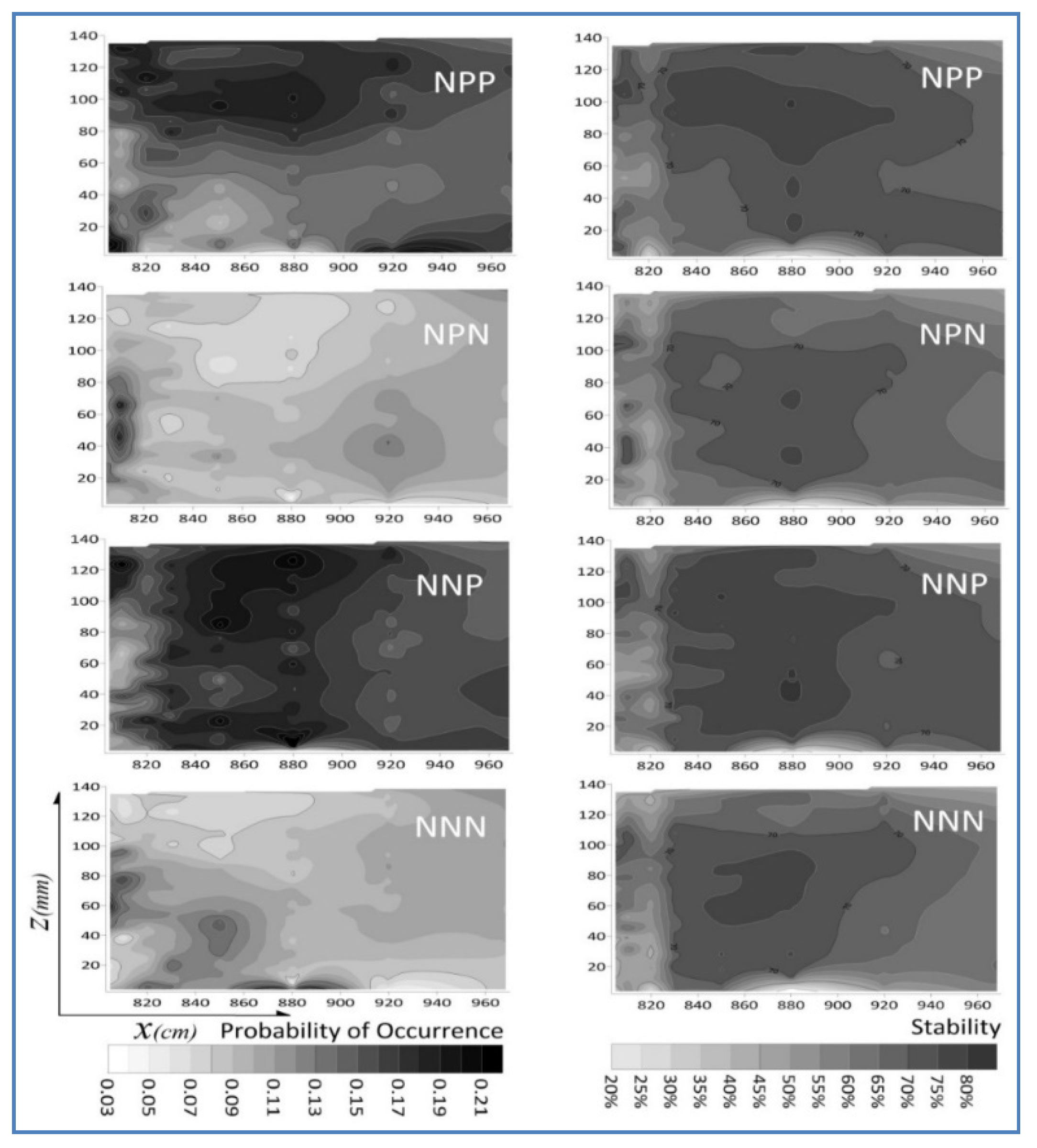
The second zone is shaped from the top edge of the vegetation patch and covers all upper parts of the flow (z > 80 mm or z/HV > 0.75). The dominant classes of this zone are PPN, PNN, NPP and NNP, which are outward and inward interactions. However, the classes of PPN, PNN and NPP are more dominant and also more stable in comparison to the class of NNP. In this zone, the projections of PPN and NNP on the vertical plane are contrarotating vertical vortexes that create sweep and ejection events, respectively, and erupting momentum in the right and left sides of the plane as the secondary flow in addition to the vertical momentum transition [30]. The occurrence of the sweep is responsible for the horizontal transfer of momentum towards the right side of the channel, while the occurrence of the ejection does it towards the left side. Obviously, in this procedure, the signs of both v’ and u’ vary simultaneously and create a fluctuation inward-outward series of occurrences in the horizontal plane. This fluctuation is formed from the top edge of the vegetation patch and creates the von Karman Vortex Street in the upper layer of the flow. The couple of PNN and NPP also act similarly but in the form of a fluctuating sweep-ejection series. However, because of the relatively less stability of the class PNN, the class NPP is not balanced in this zone. Therefore, it can be concluded that the dominant class of this zone in the vertical plane is in the form of ejection events created by NPP with a small margin. This is confirmed by Okamoto and Nezu (2013), who did a 2D quadrant analysis and showed this small margin of ejection dominancy in a similar zone for a submerged patch [6].
The third zone is shaped beyond the vegetation patch (z/HV < 0.75). The spatial distribution of dominant classes in this zone is more complicated. Even though some spots look like the PPP and NNP events, no obvious dominant class of occurrence is detectable in the middle and upper part of this zone. However, in the lower region of this zone (the near-bed zone), both NNP and PPN are dominant and relatively stable for 1 < x/DV < 4 (~830 < x < ~920). There is also a region with a high probability for PPP, but it is very unstable. Both NPP and PNN are also dominant and relatively stable for x/DV > 4. Similar to the second zone, the von Karman Vortex Street is detectable in this zone. In the zone x/DV = 2.7 (x = 880), where PPN and NNP have the highest rate of occurrence, the TKE drops to nil. However, the TKE increases slightly for x/DV > 4 (see Figure 4), which is related to the change of the inward-outward series to the sweep-ejection series in the horizontal plane. For x/DV > 4 and in the vertical plane, both sweep and ejection events are almost in the same prevalence, similar to 1 < x/DV < 4, where the outward and inward occurrences are comparable with results of a 2D quadrant analysis by Okamoto and Nezu (2013) [6]. For x/DV < 1, due to the stem-scale effects of the through-patch flow, a small region of PNN-NPP is detectable in the near-bed zone.
5.3. Coherent Shear Stresses behind Thevegetation Patch
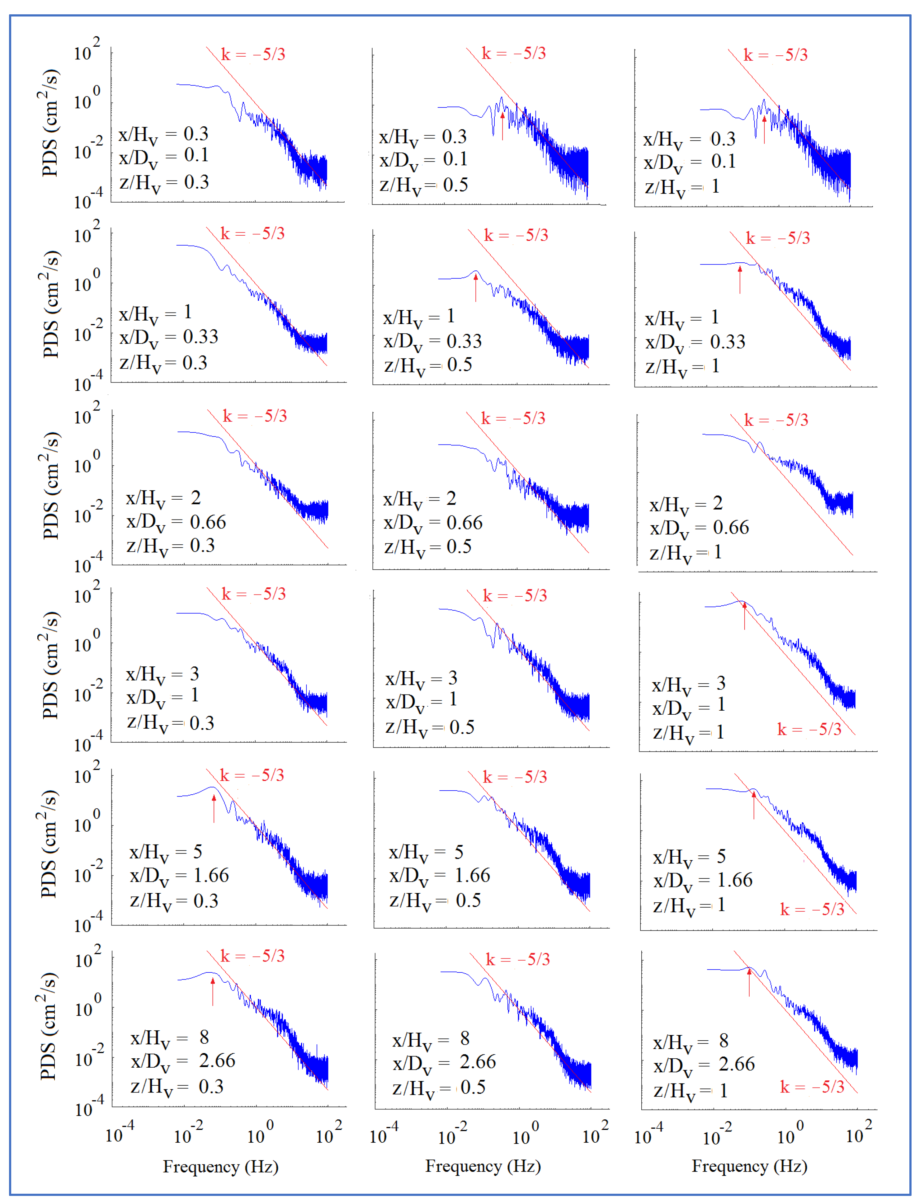
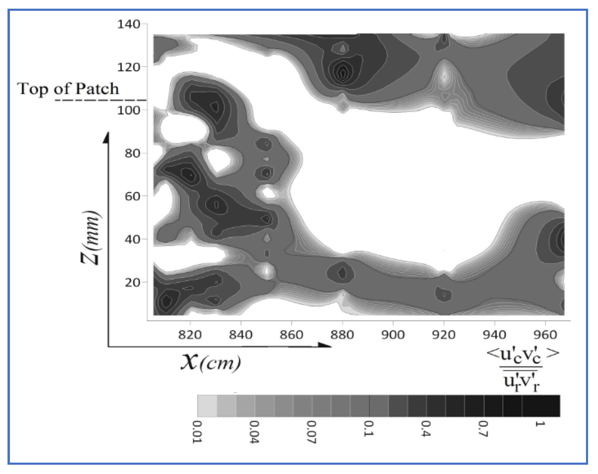
The bursting events and TKE analysis show that strong vertical vortexes lead to the diminution of the von Karman Vortex Street in the middle depth of flow. However, a part of horizontal vortexes is pushed down to the near-bed zone, and a considerable part moves up to near the surface zone. As the presence of coherent structures is associated with the presence of dominant frequency in the velocity time series, power spectra of the u component are calculated for different regions of flow behind the vegetation patch (Figure 7). The absence of peaks in the spectra in the middle region of the flow confirms that the von Karman vortex street is pushed towards the near-bed and near-surface zones. The frequency of vortex shedding in the stem-scale zone was considerably higher than that in the non-stem scale regions, as expected. The frequency of the vortex shedding in both the near-bed zone and near-surface zone is 0.07–0.11 Hz. Then, both and are calculated for regions where the von Karman vortex street is detected (Figure 8). A Matlab@ code was used to calculate the phase velocity and its deflection for the dominant frequency at each point. The coherent horizontal momentum transfer, which is triggered by the coherent horizontal vortexes, continues to happen in both the near-surface zone and near-bed zone. However, the magnitude of the phenomena is considerably low in the near-bed zone. In addition, the presence of the von Karman vortex in the near-bed zone is associated with the dominancy of NNP and PPN events that reveals the relatively strong horizontal momentum transfer events in this region. In contrast, the traditional 2D quadrant analysis is not capable of detecting this behavior of the flow in such cases. The previous research, such as Siddique et al. (2008) and Liu et al. (2018), indicate the presence of von Karman vortexes occurred in Hv/H > 0.55~0.7 [3,11]. However, they used TKE variation and visual approaches to detect the formation of von Karman vortexes in the horizontal plane. In contrast, the coherent shear stress analysis reveals that although the formation of horizontal vortexes in the near-bed zone is postponed by a strong vertical vortex behind the patch, the formation of the near-bed horizontal vortexes is not disturbed by the vertical vortex in a small patch. All results indicate that the von Karman vortexes must be also considered as a vertically distributed phenomenon that may have different behaviors in altered depths.
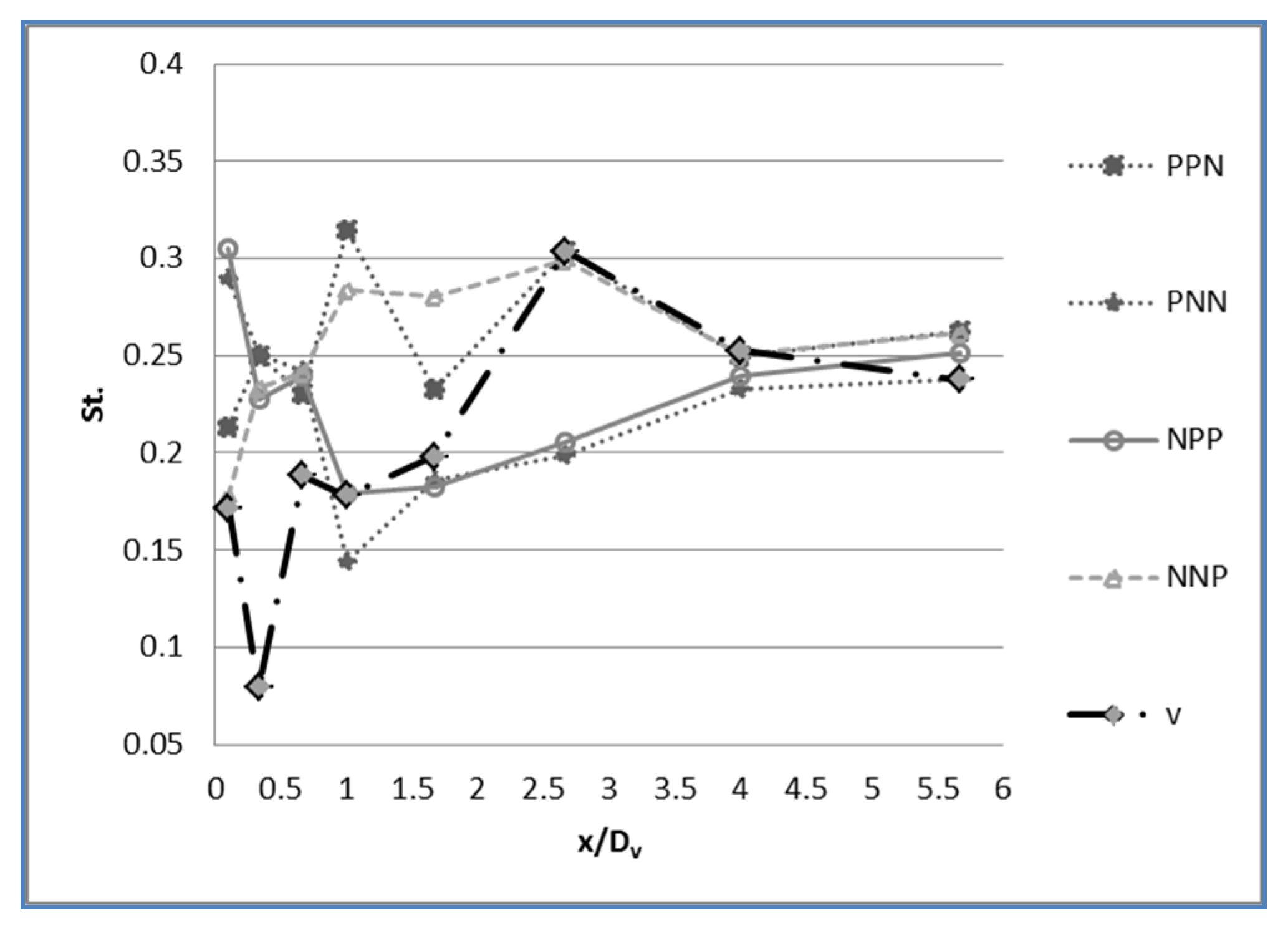
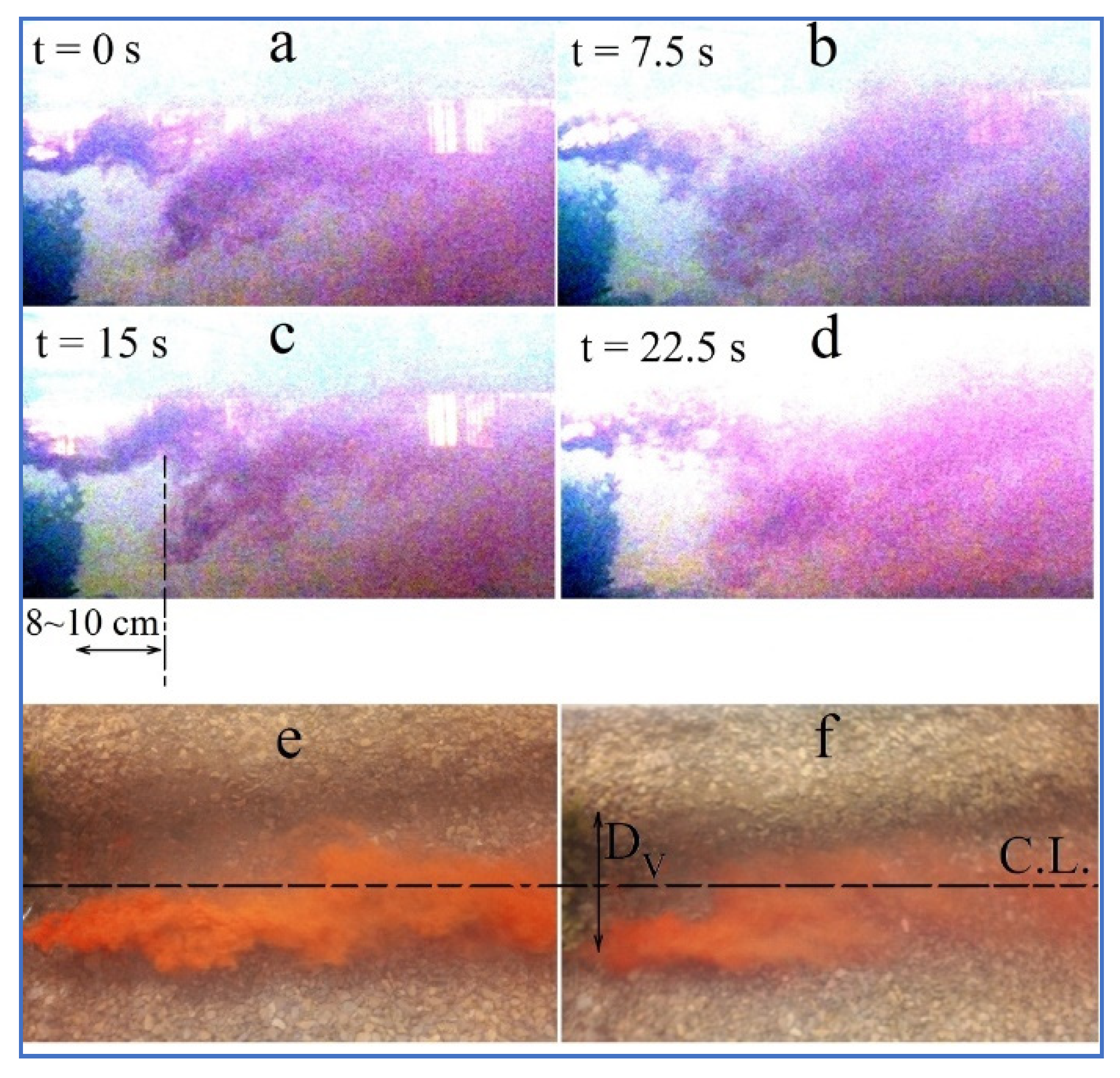
The frequency of the vortex shedding in the downstream of a barrier is generally calculated via Strouhal number. This dimensionless parameter is defined as St = f L/U, where f is the frequency of the vortex shedding, L is the characteristic length of the barrier and U is the upstream velocity. While the Strouhal number is calculable via Reynolds number and the shape of the barrier, the reported values for the vegetation patches are around 0.2 [5,31]. Therefore, the frequency of the vortex shedding is available from the pre-calculated Strouhal number for a particular characteristic length and upstream velocity. The dimensionless Strouhal number is calculated for the frequency of the bursting events and (Figure 9). Obviously, the dominant frequency of is comparable with some classes of the bursting events, particularly NNP and PPN for x/Dv > 2.5. However, the Strouhal number for all illustrated are similar beyond x/Dv > 4 (St ≈ 0.25). While the dominant frequency was 0.07–0.3 Hz, the period of the von Karman vortexes is evaluated as 3.5–15 s. In contrast, Liu et al. (2018) considered a period of 8–13 s [3]. Therefore, a 30 s video was taken to evaluate the length of the wake behind the vegetation patch (Figure 10). The wake length is estimated at around (0.8–1) Hv, which is the same as that of previous researches.
6. Conclusions
In this paper, the model vegetation patches are used to model vegetation patches in natural rivers. The characteristics of the formation of vortex structures in the wake of submerged vegetation patches have been studied. The results of the TKE and streamwise velocity indicate that both horizontal and vertical vortexes formed behind the vegetation patch for a channel bed that was partially covered with vegetation. However, strong vertical vortexes lead to the diminution of the von Karman Vortex Street. With the presence of the smallest vegetation patch in the channel bed (case 4, Lv/Dc = 0.44 and Dv/Dc = 0.33), the through-patch flow near the channel bed leads to the formation of vortex toward the downstream; however, the von Karman vortex street is presented near the channel bed. Although previous researches indicated the formation of von Karman vortexes beyond some patches with particular geometric scales, the vertical distribution of horizontal vortexes has not been investigated as a particular topic. The results of a 3D analysis of the bursting events show that the von Karman vortex street is fragmented in two parts in the near-bed zone (the weak part) and near-surface zone (the strong part), where the horizontal vortexes are associated with a particular bursting event in each zone. The formation of the near-surface von Karman vortexes is affected considerably by the vertical vortexes behind the patch; however, the near-bed horizontal vortexes almost remain intact.
The results of this study are confirmed by the behavior of the power spectra as well as the coherent shear stresses. The Strouhal number of about 0.25 is also calculated based on the frequencies of the associated bursting events and fluctuations of the lateral velocity component.
Author Contributions
M.K.: Laboratory works, methodology, software and writing—original draft preparation; H.A.: Laboratory supervisory, methodology and validation; J.S.: methodology and writing reviewing. All authors have read and agreed to the published version of the manuscript.
Funding
This research received no external funding.
Institutional Review Board Statement
Not applicable.
Informed Consent Statement
Not applicable.
Data Availability Statement
The data are available in the case that it is required.
Acknowledgments
Special thanks to G. Ghodrati Amiri for providing the laboratory devices and Esmaeel Dodangeh for his contribution in laboratory setup.
Conflicts of Interest
The authors declare no conflict of interest.
References
- Nikora, V.; Larned, S.; Nikora, N.; Debnath, K.; Cooper, G.; Reid, M. Hydraulic resistance due to aquatic vegetation in small streams: Field study. J. Hydraul. Eng. 2008, 134, 1326–1332. [Google Scholar] [CrossRef]
- Gurnell, A.M.; Bertoldi, W.; Corenblit, D. Changing river channels: The roles of hydrological processes, plants and pioneer fluvial landforms in humid temperate, mixed load, gravel bed rivers. Earth-Sci. Rev. 2012, 111, 129–141. [Google Scholar] [CrossRef]
- Liu, C.; Hu, Z.; Lei, J.; Nepf, H. Vortex structure and sediment deposition in the wake behind a finite patch of model submerged vegetation. J. Hydraul. Eng. 2018, 144, 04017065. [Google Scholar] [CrossRef]
- Caroppi, G.; Västilä, K.; Järvelä, J.; Rowiński, P.M.; Giugni, M. Turbulence at water-vegetation interface in open channel flow: Experiments with natural-like plants. Adv. Water Resour. 2019, 127, 180–191. [Google Scholar] [CrossRef]
- Afzalimehr, H.; Riazi, P.; Jahadi, M.; Singh, V.P. Effect of vegetation patches on flow structures and the estimation of friction factor. ISH J. Hydraul. Eng. 2019, 1–11. [Google Scholar] [CrossRef]
- Okamoto, T.A.; Nezu, I. Spatial evolution of coherent motions in finite-length vegetation patch flow. Environ. Fluid Mech. 2013, 13, 417–434. [Google Scholar] [CrossRef]
- Vandenbruwaene, W.; Temmerman, S.; Bouma, T.J.; Klaassen, P.C.; De Vries, M.B.; Callaghan, D.P.; Van Steeg, P.; Dekker, F.; Van Duren, L.A.; Martini, E.; et al. Flow interaction with dynamic vegetation patches: Implications for biogeomorphic evolution of a tidal landscape. J. Geophys. Res. Earth Surf. 2011, 116. [Google Scholar] [CrossRef] [Green Version]
- Bretón, F.; Baki, A.B.M.; Link, O.; Zhu, D.Z.; Rajaratnam, N. Flow in nature-like fishway and its relation to fish behavior. Can. J. Civ. Eng. 2013, 40, 567–573. [Google Scholar] [CrossRef]
- Golpira, A.; Baki, A.B.; Zhu, D.Z. Turbulent Events around an Intermediately Submerged Boulder under Wake Interference Flow Regime. J. Hydraul. Eng. 2021, 147, 06021005. [Google Scholar] [CrossRef]
- Zong, L.; Nepf, H. Vortex development behind a finite porous obstruction in a channel. J. Fluid Mech. 2012, 691, 368–391. [Google Scholar] [CrossRef]
- Sadeque, M.A.; Rajaratnam, N.; Loewen, M.R. Flow around cylinders in open channels. J. Eng. Mech. 2008, 134, 60–71. [Google Scholar] [CrossRef]
- Folkard, A.M. Hydrodynamics of model Posidonia oceanica patches in shallow water. Limnol. Oceanogr. 2005, 50, 1592–1600. [Google Scholar] [CrossRef]
- Perera, M.D.A.E.S. Shelter behind two-dimensional solid and porous fences. J. Wind Eng. Ind. Aerodyn. 1981, 8, 93–104. [Google Scholar] [CrossRef]
- Chen, Z.; Ortiz, A.; Zong, L.; Nepf, H. The wake structure behind a porous obstruction and its implications for deposition near a finite patch of emergent vegetation. Water Resour. Res. 2012, 48, 9. [Google Scholar] [CrossRef]
- Chen, Z.; Jiang, C.; Nepf, H. Flow adjustment at the leading edge of a submerged aquatic canopy. Water Resour. Res. 2013, 49, 5537–5551. [Google Scholar] [CrossRef]
- Kabiri, F.; Afzalimehr, H.; Sui, J. Flow structure over a wavy bed with vegetation cover. Int. J. Sediment Res. 2017, 32, 186–194. [Google Scholar] [CrossRef]
- Sui, J.; Faruque, M.A.; Balachandar, R. Local scour caused by submerged square jets under model ice cover. J. Hydraul. Eng. 2009, 135, 316–319. [Google Scholar] [CrossRef]
- Jafari, R.; Sui, J. Velocity Field and Turbulence Structure around Spur Dikes with Different Angles of Orientation under Ice Covered Flow Conditions. Water 2021, 13, 1844. [Google Scholar] [CrossRef]
- Hussain, A.F. Role of coherent structures in turbulent shear flows. Proc. Indian Acad. Sci. Sect. C Eng. Sci. 1981, 4, 129–175. [Google Scholar]
- Afzalimehr, H.; Moghbel, R.; Gallichand, J.; Sui, J. Investigation of turbulence characteristics in channel with dense vegetation. Int. J. Sediment Res. 2011, 26, 269–282. [Google Scholar] [CrossRef]
- Devi, T.B.; Kumar, B. Channel hydrodynamics of submerged, flexible vegetation with seepage. J. Hydraul. Eng. 2016, 142, 04016053. [Google Scholar] [CrossRef]
- Huai, W.X.; Zhang, J.; Katul, G.G.; Cheng, Y.G.; Tang, X.; Wang, W.J. The structure of turbulent flow through submerged flexible vegetation. J. Hydrodyn. 2019, 31. [Google Scholar] [CrossRef]
- Zamani, M.; Afzalimehr, H.; Jahadi, M.; Singh, V.P. Flow structure over bed form with flexible vegetation patches. ISH J. Hydraul. Eng. 2021, 1–7. [Google Scholar] [CrossRef]
- Przyborowski, Ł.; Łoboda, A.M. Identification of coherent structures downstream of patches of aquatic vegetation in a natural environment. J. Hydrol. 2021, 596, 126123. [Google Scholar] [CrossRef]
- Keshavarzi, A.R.; Gheisi, A.R. Stochastic nature of three dimensional bursting events and sediment entrainment in vortex chamber. Stoch. Environ. Res. Risk Assess. 2006, 21, 75–87. [Google Scholar] [CrossRef]
- Keshavarzi, A.; Melville, B.; Ball, J. Three-dimensional analysis of coherent turbulent flow structure around a single circular bridge pier. Environ. Fluid Mech. 2014, 14, 821–847. [Google Scholar] [CrossRef]
- Termini, D. Experimental Analysis of Horizontal Turbulence of Flow over Flat and Deformed Beds. Arch. Hydro-Eng. Environ. Mech. 2015, 62, 77–99. [Google Scholar] [CrossRef] [Green Version]
- Termini, D.; Sammartano, V. Analysis of the role of turbulent structure in bed-forms formation in a rectilinear flume. In Proceedings of the 32nd Congress of IAHR, “Harmonizing the Demands of Art and Nature in Hydraulics”, Venice, Italy, 1–6 July 2007. [Google Scholar]
- Termini, D.; Sammartano, V. Experimental observation of horizontal coherent turbulent structures in a straight flume. In Proceedings of the 2019 River Coast. Estuarine Morphodynamics—RCEM 2019, Santa Fe City, Argentina, 21–29 September 2009. [Google Scholar]
- Wang, H.; Peng, G.; Chen, M.; Fan, J. Analysis of the interconnections between classic vortex models of coherent structures based on DNS data. Water 2019, 11, 2005. [Google Scholar] [CrossRef] [Green Version]
- Graf, W.H.; Altinakar, M.S. Fluvial Hydraulics: Flow and Transport Processes in Channels of Simple Geometry; No. 551.483 G7; Wiley: Hoboken, NJ, USA, 1998. [Google Scholar]
Figure 1.
Bursting events in the octant analysis and right-wing and left-wing classification of the events (PNN event which is located in the left wing is not seen in this angle of view).
Figure 1.
Bursting events in the octant analysis and right-wing and left-wing classification of the events (PNN event which is located in the left wing is not seen in this angle of view).

Figure 2.
The transition probability matrix for the octant analysis; the values on the main diagonal show the probability of self-repeating of an event in the same octant class.
Figure 2.
The transition probability matrix for the octant analysis; the values on the main diagonal show the probability of self-repeating of an event in the same octant class.

Figure 3.
(A) The layout of the experimental device, (B) a sample of vegetation patches (120 × 90 cm, DV/DC = 1), (C) a sample of a vegetation patch in a natural gravel-bed river (Marbor River, Iran), (D) a sample of bed materials, (E) a single synthetic plant used to simulate patch, and (F) a sketch of the experimental set-up (Not to scale).

Figure 4.
Normalized TKE and streamwise velocity behind 4 different patch layouts near channel bed (z/Hv = 0), at the middle height of patch (z/Hv = 0.5) and top of patch (z/Hv = 1).
Figure 4.
Normalized TKE and streamwise velocity behind 4 different patch layouts near channel bed (z/Hv = 0), at the middle height of patch (z/Hv = 0.5) and top of patch (z/Hv = 1).

Figure 5.
Probability of the occurrence and stability of octant classes PPP, PPN, PNP and PPP behind the vegetation patch. The end of the patch is located in x = 800. The height of patches is 105 ± 5 mm. The values are shown up to the level of the maximum domain of ADV capability (~140 mm).
Figure 5.
Probability of the occurrence and stability of octant classes PPP, PPN, PNP and PPP behind the vegetation patch. The end of the patch is located in x = 800. The height of patches is 105 ± 5 mm. The values are shown up to the level of the maximum domain of ADV capability (~140 mm).

Figure 6.
Probability of the occurrence and stability of octant classes NPP, NPN, NNP and NPP behind the vegetation patch.
Figure 6.
Probability of the occurrence and stability of octant classes NPP, NPN, NNP and NPP behind the vegetation patch.

Figure 7.
Power spectra behind vegetation patch for case 4; the arrow indicates the peak frequency associated with vortex shedding behind the patch, which varied from 0.07 to 0.11 Hz for main vortexes and is around 0.4 Hz for stem-scale vortexes.
Figure 7.
Power spectra behind vegetation patch for case 4; the arrow indicates the peak frequency associated with vortex shedding behind the patch, which varied from 0.07 to 0.11 Hz for main vortexes and is around 0.4 Hz for stem-scale vortexes.

Figure 8.
Values of in the near-bed and near-surface zones; note that the white-colored area is where that no dominant frequency is detectable for velocity time series.
Figure 8.
Values of in the near-bed and near-surface zones; note that the white-colored area is where that no dominant frequency is detectable for velocity time series.

Figure 9.
Strouhal Number calculated via the frequency of the bursting events and v.

Figure 10.
(a–d) Formation of the vertical vortexes and the wake zone behind the vegetation patch for case 4; (e) formation of the horizontal vortexes behind the patch with dike injection at z/Hv = 1 and (f) near the bed. Note that the injection point is located at the right edge of the patch for the horizontal vortexes.


Table 1.
Three-dimensional analysis of bursting events in the octant analysis.
| Classes of Bursting Events | Class Name | Sign of Fluctuating Velocities | ||
|---|---|---|---|---|
| Right-wing outward interaction | PPP | + | + | + |
| Right-wing sweep | PPN | + | + | − |
| Left-wing outward interaction | PNP | + | − | + |
| Left-wing sweep | PNN | + | − | − |
| Right-wing ejection | NPP | − | + | + |
| Right-wing inward interaction | NPN | − | + | − |
| Left-wing ejection | NNP | − | − | + |
| Left-wing inward interaction | NNN | − | - | − |
Table 2.
Experimental parameters for the four cases discussed in this study.
| Case | Q (Discharge, L/s) | n/m2 (Number of Veg. Per Square Meter) | LV (Length of Patch, cm) | DV (Width of Patch, cm) | HV (Height of Patch, cm) |
|---|---|---|---|---|---|
| 1 | 31 | 611.1 | 120 | 90 | 10 |
| 2 | 31 | 611.1 | 90 | 60 | 10 |
| 3 | 31 | 611.1 | 60 | 45 | 10 |
| 4 | 31 | 611.1 | 40 | 30 | 10 |
Publisher’s Note: MDPI stays neutral with regard to jurisdictional claims in published maps and institutional affiliations. |
© 2021 by the authors. Licensee MDPI, Basel, Switzerland. This article is an open access article distributed under the terms and conditions of the Creative Commons Attribution (CC BY) license (https://creativecommons.org/licenses/by/4.0/).
Share and Cite
MDPI and ACS Style
Kazem, M.; Afzalimehr, H.; Sui, J. Formation of Coherent Flow Structures beyond Vegetation Patches in Channel. Water 2021, 13, 2812. https://doi.org/10.3390/w13202812
AMA Style
Kazem M, Afzalimehr H, Sui J. Formation of Coherent Flow Structures beyond Vegetation Patches in Channel. Water. 2021; 13(20):2812. https://doi.org/10.3390/w13202812
Chicago/Turabian StyleKazem, Masoud, Hossein Afzalimehr, and Jueyi Sui. 2021. "Formation of Coherent Flow Structures beyond Vegetation Patches in Channel" Water 13, no. 20: 2812. https://doi.org/10.3390/w13202812
Note that from the first issue of 2016, this journal uses article numbers instead of page numbers. See further details here.