1. Introduction
Evaporation is one of the main components of hydrology, and accurate estimation of evaporation plays an essential role in estimating the water balance of basins, designing and managing irrigation systems, and managing water resources [
1,
2,
3,
4,
5].
There are two types of methods, direct and indirect, for estimating evaporation [
6,
7]. Pan evaporation is one of the direct methods commonly used to determine evaporation from free water surfaces in most parts of the world [
8]. Pan evaporation is also used for determining crop water requirements, irrigation scheduling, rainfall–runoff modeling, and computation of water balance components [
5]. In recent years, numerous methods and experimental relationships have been developed for indirectly simulating evaporation [
9,
10]. Over the years, various studies have sought to identify linear experimental relationships [
11,
12,
13] and non-linear experimental relationships [
14,
15,
16,
17,
18,
19,
20] as indirect methods to simulate evaporation from free water surfaces. Some of these experimental relationships are listed in
Table S1 in Supplementary Material (SM). Four input meteorological variables (air temperature, relative humidity [
13], wind speed, and vapor pressure) have been used in most cases [
12,
13,
21,
22]. On the other hand, Filimonova and Trubetskova [
23] used two variables (temperature and relative humidity), Poormohammadi et al. [
24] used two parameters (temperature and vapor pressure), and Patra [
25] used only temperature in their experimental relationships. Moreover, copious studies have assessed the sensitivity of input parameters in simulating evaporation (
Table S2 in SM). These studies have shown that temperature, relative humidity, wind speed, and sunshine hours are the most sensitive parameters [
26,
27]. In addition, artificial intelligence has been widely used for modeling and simulating pan evaporation [
28,
29,
30,
31,
32,
33]. In recent years, multilayer perceptron neural network (MLP-NN) has become one of the most useful artificial intelligence tools in simulating pan evaporation, and its ability for simulation of pan evaporation has been verified in many studies e.g., Alsumaiei [
29]; Pandey et al. [
28]; Ashrafzadeh et al. [
34]; Patle et al. [
35], as listed in
Table S3 in SM.
In general, the studies cited above have left four research gaps in the simulation of evaporation: (i) A limited geographical area has been used to develop these methods, which can result in errors in applying the methods. (ii) The structure of the experimental relationships developed does not have the desired simplicity, and users cannot easily use them. Moreover, using neural networks is not user-friendly and accessible for all users. (iii) In most proposed relationships, the vapor pressure variable is a required input, but this parameter is not commonly measured at all weather stations. (iv) The methods lack the ability to simulate evaporation under different climatic conditions. For instance, Ivanov’s relationship is suggested for dry and semi-dry climates [
25,
36,
37] and Penman’s relationship for coastal regions with humid and very humid conditions [
38]. In the present study, Iran was selected as the study region for the development of two comprehensive and practical methods for simulating pan evaporation under different climatic conditions. Iran, which is one of the largest countries in the Middle East, has six different climate types. Potential evaporation is greater than precipitation in the country [
39], and simulating evaporation with high accuracy can play an important role in national water resources management.
The present study provided several advantages and innovations compared with previous research, including: (i) The choice of the study region, as Iran covers a vast area and has six different climate types (dry, semi-dry, Mediterranean, humid, semi-humid, very humid), (ii) introduction of two practical and simple graphs as the first method and a simple basic relationship with six climatic correction coefficients as the second method to simulate pan evaporation for the six climate types in Iran, as both methods are more comprehensive, yet simpler to apply, than those in previous studies; and (iii) use of common meteorological data available from all weather stations in Iran in the comprehensive methods for simulating pan evaporation.
The remainder of this paper is organized as follows:
Section 2 describes the study area, and
Section 3 introduces the methodology used to develop evaporation modeling. Results are presented in
Section 4 and discussed in
Section 5, while some conclusions are presented in
Section 6.
2. Study Area
Iran is located in West Asia, and in terms of the geographical location lies in the Northern Hemisphere between 25 to 40 degrees north and 44 to 63.5 degrees east [
40]. The territory of Iran comprises about 1,650,000 km
2, and most regions have dry to semi-dry climatic conditions [
40]. Climatic conditions are affected by two important mountain chains, Alborz and Zagros, which extend from northwest to eastern and southern regions of Iran, respectively, and represent a change in altitude from −25 to 5600 m above mean sea level [
41]. Differences in climatic conditions also exist due to the uneven distribution of precipitation and humidity in the country [
41]. The northern part is coastal and humid, with heavy precipitation due to the Alborz mountains, while central, southern, and eastern parts are dry with frequent droughts. Most parts in the west, northwest, and southwest of Iran have a semi-dry climate and above-average precipitation due to the obstruction of rain-producing air masses by the Zagros mountain chain [
42].
A significant proportion of precipitation in Iran is produced by the Mediterranean system, which moves from west to east through the action of westerly winds. Mean annual precipitation in Iran is about 240 mm/year, equivalent to one-third of the global average [
43]. Annual precipitation ranges from approximately 1800 mm for the Caspian Sea coastal plains to 400 mm for the Alborz and Zagros Mountains [
44] but is lower than 100 mm following local topology in the internal plains located in Iran’s eastern and central parts [
44]. In terms of temperature, most regions of Iran are affected by the tropical high-pressure system, which results in very hot and dry summers in much of Iran [
44]. In the cold-season areas in Iran, ranging from 10–70° North and 10–80° East, important climatic indices include the Arctic, Central Asia, Western Europe, and Anatolia to north Caspian indices [
45]. The cold temperature areas of Iran lie mainly along the Zagros Mountains, in the northwest, and in small parts of the northeast. There is a strong spatial distribution of hot and cold temperature areas in Iran, with an obvious role of greater altitude in cold areas [
46].
Since most parts of Iran experience dry and semi-dry climatic conditions, evaporation is an important meteorological variable [
47,
48,
49]. Drought is a natural and repeatable phenomenon that can cause severe crises, and the most critical factors in drought development are precipitation and evaporation [
50]. In recent years, droughts have become more frequent and severe in Iran [
50,
51,
52]. Drought is a growing problem in Iran because excessive groundwater use during drought conditions causes annual evaporation to exceed the annual renewable water supply due to precipitation [
40].
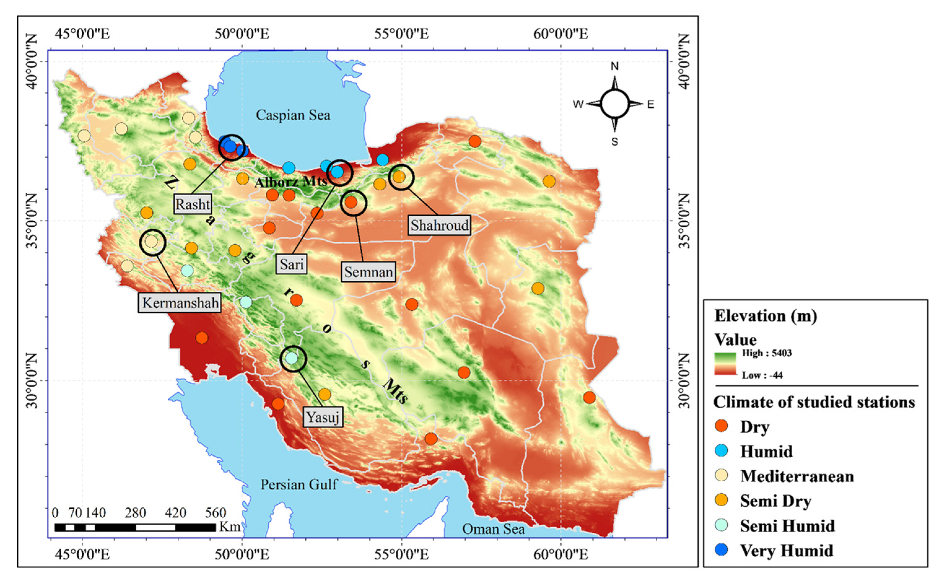
In this study, pan evaporation in Iran was simulated using the MLP-NN neuron and genetic algorithm optimization model. For this purpose, observed data from 38 synoptic weather stations in Iran were selected to represent the six different climate types (dry, semi-dry, Mediterranean, semi-humid, humid, very humid). Data from six synoptic weather stations (Semnan, Shahroud, Yasuj, Kermanshah, Sari, and Rasht) were used to develop experimental relationships, and data from the remaining 32 stations were used to validate these experimental relationships. The geographical location and climate conditions at the selected synoptic weather stations are shown in
Figure 1. As can be seen, there is a humid and very humid climate in northern Iran and the coastal region along the Caspian Sea, while Mediterranean and semi-humid climatic conditions are found mainly in the west and northwest of Iran, and southwestern regions have a dry or semi-dry climate. The number of selected synoptic weather stations with dry, semi-dry, Mediterranean, semi-humid, humid, and very humid climatic conditions were 13, 9, 4, 3, 3, and 6, respectively. Because significant regions of Iran are located in dry and semi-dry regions, greater number of synoptic weather stations were selected in these areas.
3. Materials and Methods
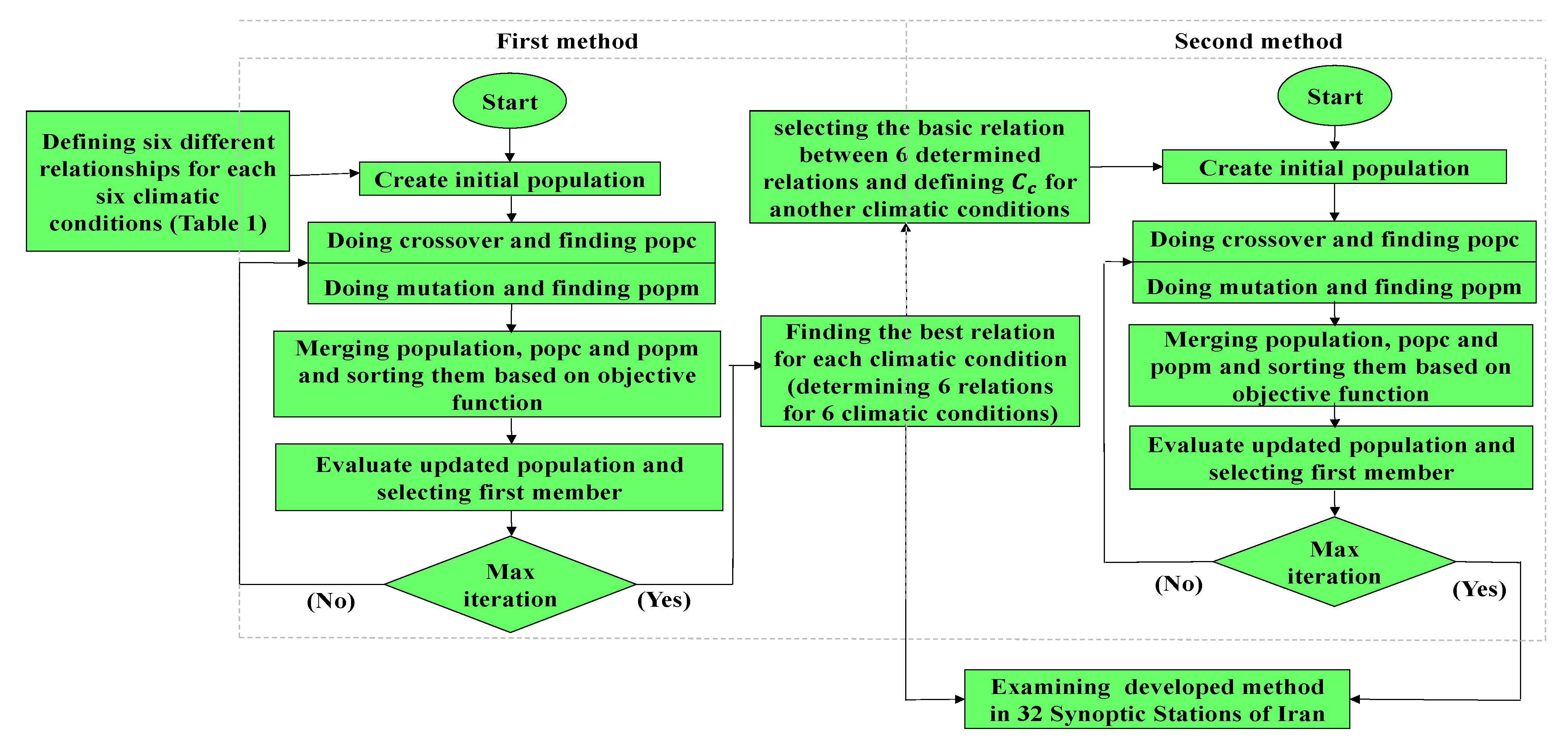
Two methods for simulating pan evaporation were developed. The steps in the first method were as follows: (1) Six synoptic weather stations were selected in Iran, that these stations have six different types of climatic conditions (
Figure 1). (2) Three experimental relationships (linear, quadratic, and cubic) were defined using a MLP-NN neuron. These relationships have two different input combinations (two-parameter and four-parameter) for each selected synoptic weather station (i.e., type of climatic conditions). The structure and input combination of these relationships are shown in
Table 1. Therefore, 36 experimental relations were defined for the six different climate types considered for Iran (based on the De Martonne method), and their coefficients were determined using the genetic algorithm optimization model. (3) The ability of the relationships to simulate evaporation was compared, and the best relationship was selected for each climate type. Finally, the outputs of these six best-performing relationships were presented in the form of a three-dimensional graph to simplify interpretation.
The steps in the second method were as follows: (1) Among the six relationships selected when developing the first method, that with the greatest ability to simulate evaporation in its relevant climatic conditions was selected as the basic experimental relation. (2) Six climatic correction coefficients (
) were defined, one for each of six types of climatic conditions, and evaporation in each climate type was simulated by multiplying by its coefficient (
) in the basic experimental relationship. The value of these coefficients (
) was determined using the genetic algorithm optimization model. (3) Finally, both methods were verified using data from 32 synoptic weather stations in Iran, and the results were compared.
Figure 2 presents an outline of the steps involved in the work, which are discussed in more detail in
Section 3.1,
Section 3.2,
Section 3.3 and
Section 3.4.
3.1. The De Martonne Method for Climate Classification
In the De Martonne method, the dryness index is calculated as:
where
P is mean annual precipitation (mm),
T is mean annual temperature (°C), and
I is dryness (De Martonne) coefficient. Based on the De Martonne drought coefficient values, climatic conditions in Iran are categorized into dry, semi-dry, Mediterranean, semi-humid, humid, and very humid (
Table 2).
3.2. Genetic Algorithm Optimization Model
The genetic algorithm is an evolutionary algorithm employed for optimizing and effectively searching huge spaces based on genes and chromosomes [
53]. The search includes four steps: (i) The initial population containing a set of chromosomes forms is established; (ii) the value of each member is determined by defining an objective function, and new members are generated using genetic operators, which include the production of offspring from selective parents, mutation on the last population members, and gradual evolution [
54]; (iii) selection is conducted considering the fitness level of the members, and several most fit chromosomes are selected for reproduction; and (iv) genetic operators act on population members and modify and combine their genetic codes [
55].
In this study, the genetic algorithm optimization model was used for two purposes: determining the optimal weights for each mathematical relationship listed in
Table 1, and determining the climatic correction coefficients to use with the basic experimental relationship. In the genetic algorithm optimization model used, the number of parents, number of offspring, number of mutant members, mutation rate, and number of iterations was 300, 200, 90, 0.04, and 200, respectively. The roulette wheel selection method was applied to select parents from the parent population [
56]. According to the fitness function, a member of the parent population can be selected if it has a better condition regarding the fitness function value, i.e., parents whose objective function has a lower value [
57]. Equation (2) expresses the probability distribution function applied in the roulette wheel selection method:
where
P is the selection probability of any member of the parent population,
is the selection pressure of the parent population, cost represents the objective function value for the parent population, and the worst cost is the maximum value of the objective function, i.e., the family with the worst conditions for the parent population. After selecting the parents, the uniform crossover approach is used for producing the offspring, as expressed by Equations (3) and (4):
where
y1i is the first offspring,
y2it is the second offspring,
x1i is the first selected parent, and
x2i is the second selected parent.
The selection of a member from the parent population to apply the mutation operator was carried out randomly. The normal distribution was used to apply the mutation operator to the parent population. Therefore, if x
i is the gene to be mutated, the mutant gene is generated by Equations (5) and (6):
where
xinew is the mutant member,
N (0, 1) is the standard normal distribution, and
σ is the step-length of normal distribution.
3.3. MLP-NN Neuron
Three different experimental relationships (
Table 1) were defined, inspired by the processes in a MLP-NN neuron. The process inside a MLP-NN neuron is as follows: input variables are multiplied by a series of fixed weights, the values obtained are summed with a constant value, the final values are given to an activation function, and the output of the intended neuron is calculated. The activation functions employed in MLP-NN neurons include hyperbolic, exponential, Gaussian, and linear functions, and so on. The linear function is the simplest form of activation function, with the general form Y = X, which simplifies the experimental relationships suggested.
Figure 3 and Equation (7) describe the process in a MLP-NN neuron.
where
F is the activation function,
X1,
X2, and
X3 represent the input variables, and
W1,
W2, and
W3 represent the weights multiplied by inputs.
In this study, the MLP-NN neuron was designed to define three experimental relationships (linear, quadratic, and cubic). In the linear relationship, input parameters were multiplied by different weights, and then the values obtained were summed with a constant value. For the quadratic and cubic relationships, the second and third powers, respectively, of the input data were multiplied by weights, and the values obtained were summed with a constant value.
3.4. Statistical Indices for Model Evaluation
There are various measures available to evaluate models and algorithms. In the present study, the experimental relationships and the climatic correction coefficients obtained for the basic relationship were quantitatively evaluated using statistical correlation coefficient (r), Nash-Sutcliffe efficiency (
NSE), root mean square error (
RMSE), and percentage bias (
PBIAS) (Equations (8)–(11)).
where
N is the number of data,
obsi is observed daily evaporation (mm/day),
simi is simulated daily evaporation (mm/day),
is average observed evaporation (mm/day), and
is average simulated evaporation (mm/day). The correlation coefficient shows the agreement between observed and modeled values, with its value varying from zero to one (the closer to one, the more acceptable the results). NSE shows the relative difference between observed and simulated values, and its value ranges from infinitely negative to one (the closer to one, the more accurate the results) [
58]. RMSE indicates the difference between observed and simulated data. RMSE is non-negative, and a value near zero shows higher reliability of the model. PBIAS indicates the mean bias in the simulated data relative to the observed data, and thus the smaller the value, the higher the reliability of the model [
59].
4. Results
4.1. Determination of Weights of Experimental Relationships Used with Two Input Combinations (First Method)
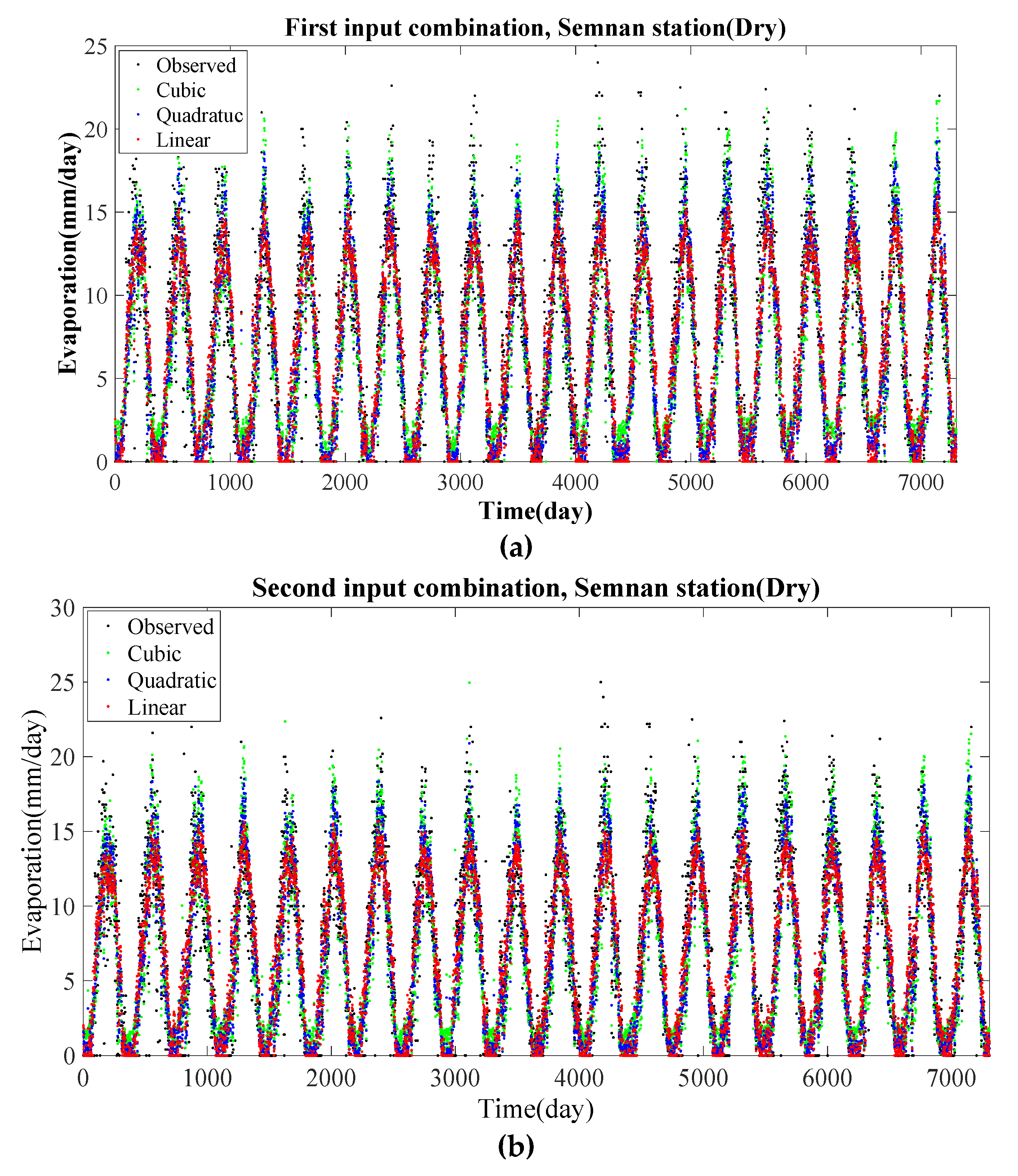
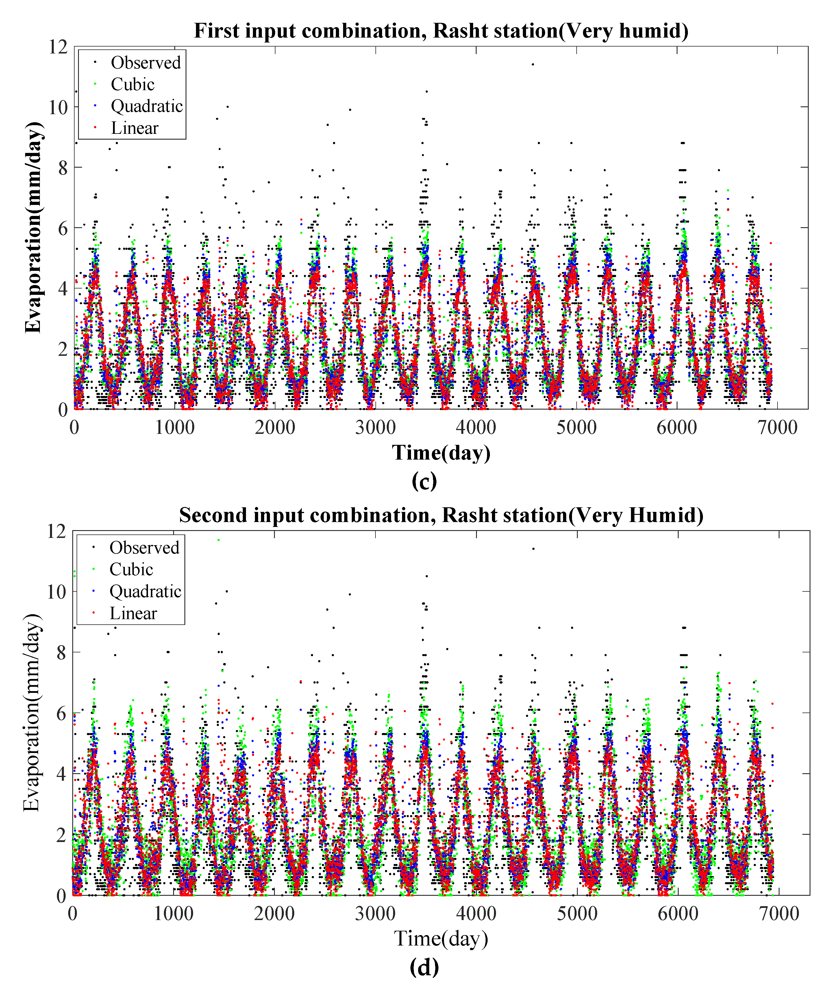
Observed and simulated pan evaporation at the six selected synoptic weather stations: Semnan (dry), Shahroud (semi-dry), Kermanshah (Mediterranean), Yasuj (semi-humid), Sari (humid), and Rasht (very humid) with the two input combinations (two-parameter, four-parameter) are shown in
Figure 4 (Semnan and Rasht) and
Figure S1 (other synoptic weather stations). As can be seen, observed evaporation and evaporation simulated using all three experimental relationships showed acceptable agreement for the six selected synoptic weather stations representing different climate types.
The values obtained for correlation coefficient (r), NSE, RMSE, and PBIAS in comparisons between observed and simulated evaporation using the three types of experimental relationships and two input combinations are shown in
Table S5 in SM. Based on the values obtained, there was little difference between the two-parameter and four-parameter input combinations. Moreover, at all six synoptic weather stations, r and NSE were higher for the quadratic experimental relationship than for the cubic and linear experimental relationships. On the other hand, RMSE and PBIAS were lower for the quadratic experimental relationship than for the other two relationships.
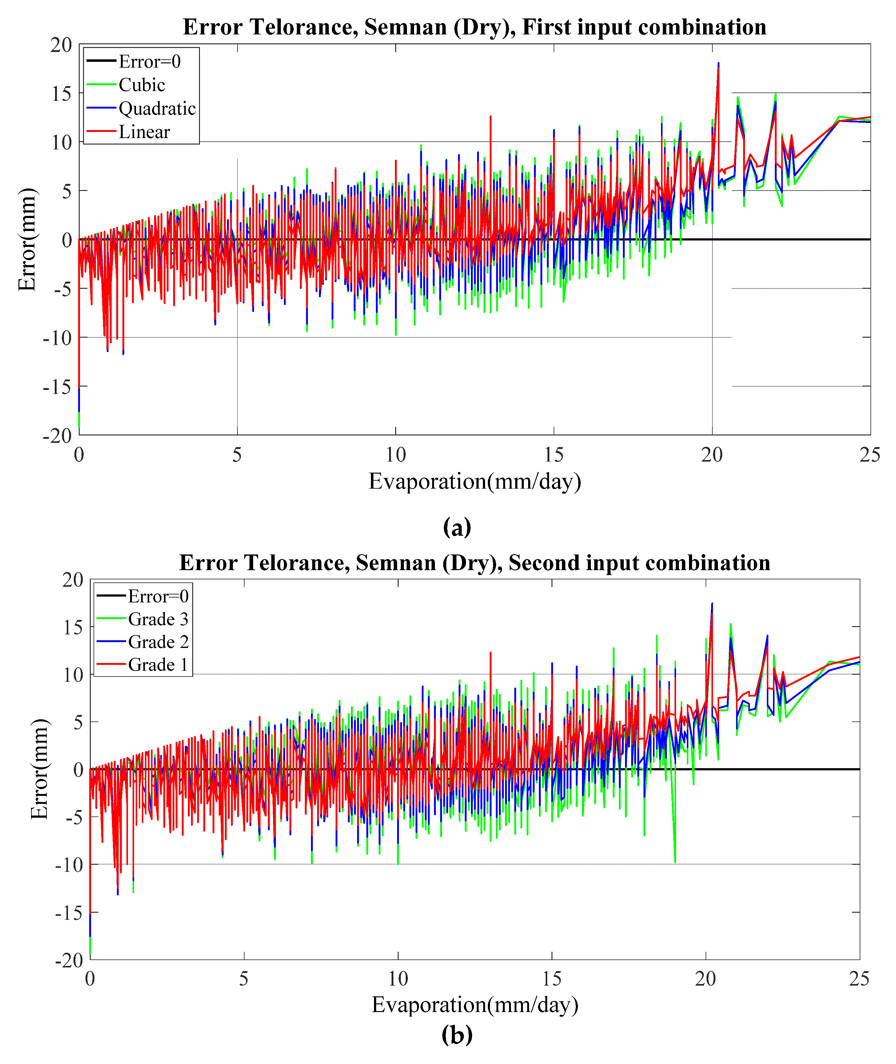
Error tolerance diagrams were created for the six selected synoptic weather stations and the two input combinations to compare the statistical coefficients of experimental quadratic relationships. In the graph for each climate type, evaporation values were arranged from low to high on the horizontal axis, and the difference between observed and simulated evaporation according to the linear, quadratic, and cubic experimental relationships was plotted on the vertical axis.
Figure 5 shows the error tolerance diagram for Semnan station, while those for the other five synoptic weather stations are shown in
Figure S2 in SM.
Based on the error tolerance values in
Figure 5 and
Figure S2, the error in simulating high evaporation was greater for the linear relationship than for the cubic and quadratic relationships with all six types of climatic conditions and both input combinations, while the error in simulating low evaporation was greater for the cubic relationship than for the quadratic and linear relationships. Therefore, the higher values of r and NSE and the lower values of RMSE and PBIAS obtained for the quadratic relationship can be related to its greater ability to simulate high evaporation than the linear relationship and its greater ability to simulate low evaporation than the quadratic relationship. The quadratic relationship was thus the best relationship for simulating evaporation in the six different climate types in Iran.
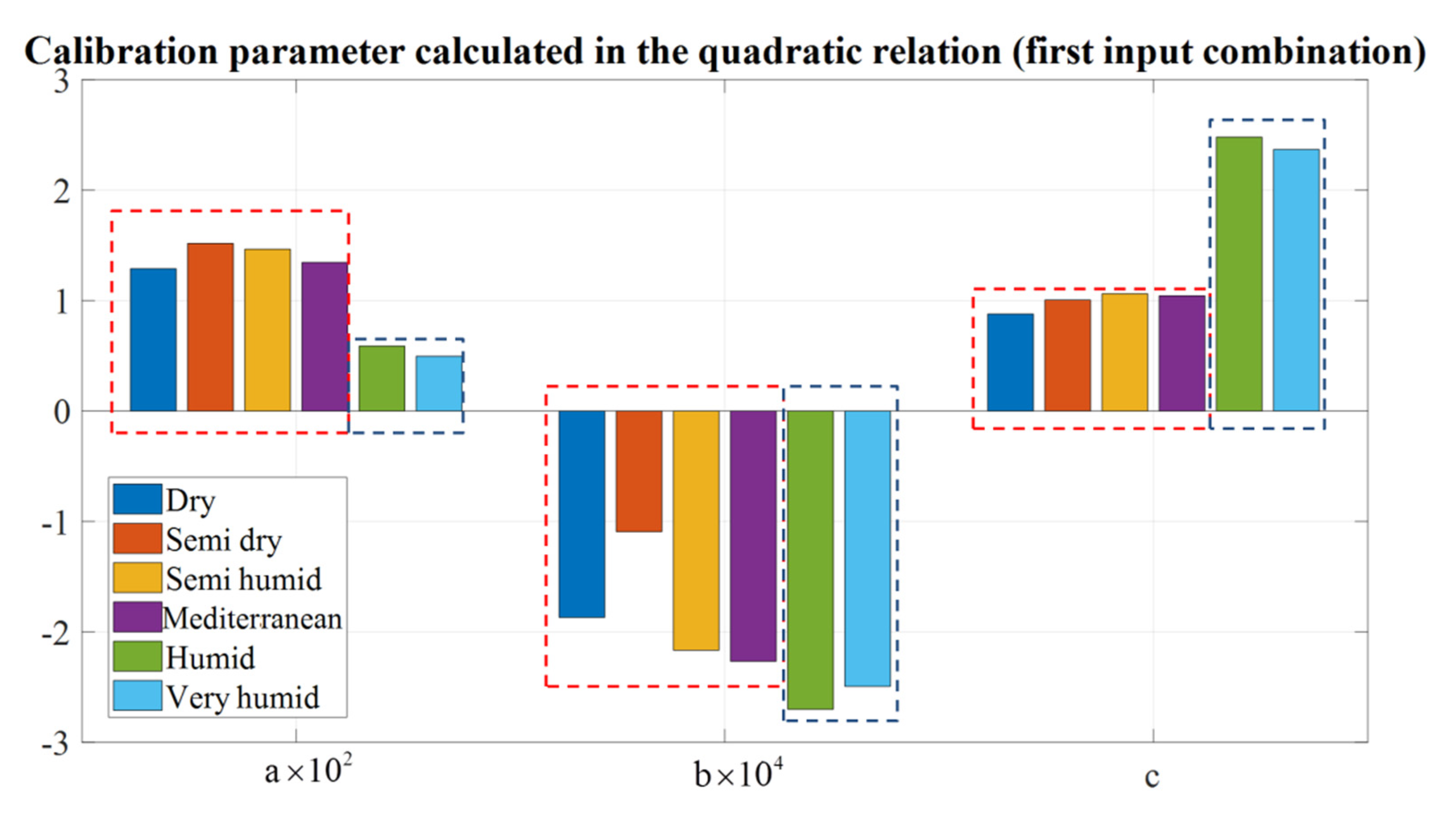
The coefficients obtained for the linear, quadratic and cubic relationships are shown in
Table S6 in SM. According to the determined weights of the best (quadratic) relationships, those for four types of climatic conditions (dry, semi-dry, semi-humid, and Mediterranean) were similar to each other but different from those for the remaining two climate types (humid and very humid), which were similar to each other. In
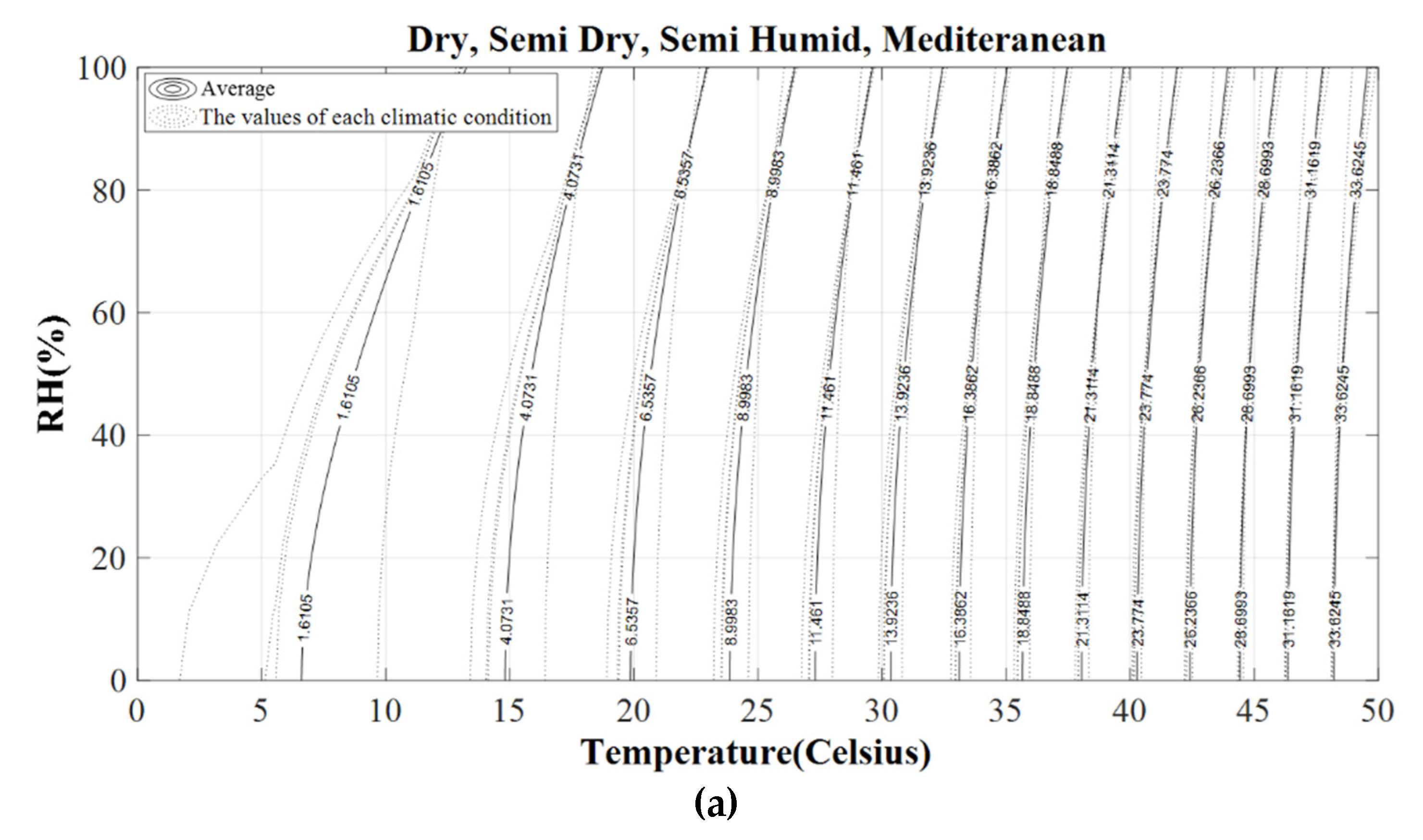
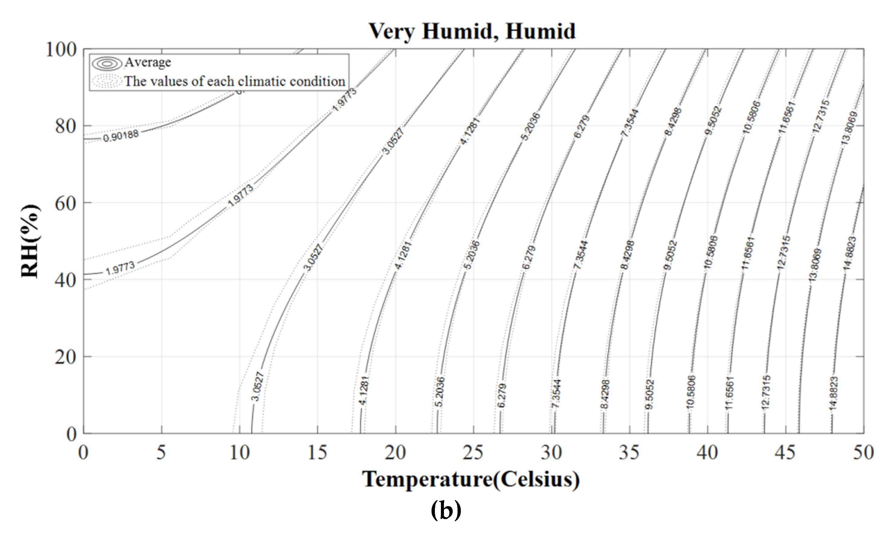
Figure 6, the similarities of the relationship weights of the dry, semi-dry, semi-humid, and Mediterranean climate types, and of the humid and very humid climate types, are shown in a bar graph for the two-parameter input combination, where pan evaporation based on two input variables (relative humidity in the range 0–100%, the temperature in the range 0–50 °C). Pan evaporation was then simulated using the experimental quadratic relationships, and simulated evaporation under each climate type was drawn as contour curves.
Figure 7a presents the results for the four synoptic weather stations with dry, semi-dry, semi-humid, and Mediterranean conditions, and
Figure 7b shows the results for the two synoptic weather stations with humid and very humid conditions. The contours of the evaporation values (dashed lines) show the approximate values of simulated evaporation for the stations. The average evaporation values for the groups of four and two stations are shown within bold lines and can be used to simulate pan evaporation. The two graphs were created using the six best experimental relationships. The variables temperature (°C) and relative humidity (%) must be extended along the horizontal and vertical axes to reach each other at a specific point, at which the value of the contour indicates pan evaporation.
4.2. Climatic Correction Coefficients for Climate Types Based on the Basic Relationship (Second Method)
The results in
Section 4.1 showed that quadratic relationships were best in simulating evaporation for the six climate types in Iran. Based on the statistical coefficients (
Table S5), the quadratic experimental relationship for the semi-dry climate showed better performance than those for other climate types and was selected as the basic experimental relationship. The climatic correction coefficient (
Cc) for semi-dry conditions was then set at 1, and the
Cc values for the dry, Mediterranean, semi-humid, humid, and very humid climate types were determined using the genetic algorithm optimization model for two input combinations.
Observed evaporation and simulated evaporation values obtained using the basic experimental relationship with the climatic correction coefficients determined for the Semnan and Rasht stations, with both input combinations, are presented in
Figure 8, while those for other climatic conditions are shown in
Figure S3. The agreement between observed evaporation and simulated evaporation in the diagrams indicates that the method is acceptable for use in six different climate types in Iran.
Table S7 shows the values of
and the values of correlation coefficient (r), NSE, PBIAS, and RMSE obtained on comparing observed and simulated evaporation with both input combinations for the six selected synoptic weather stations. The statistical coefficients confirmed that using the basic experimental relationship with six climatic correction coefficients is an acceptable approach for simulating evaporation at the six selected synoptic weather stations. Moreover, according to the statistical coefficients, there was little difference between two-parameter and four-parameter input combinations. The
values varied between 0.4 to 0.6 for humid and very-humid climates and between 0.8 and 1 for dry, semi-dry, Mediterranean, and semi-humid climates (
Table S7). Therefore, there was a significant difference between the climatic correction coefficients for these two groups, indicating that the bone experimental relationship cannot be used to simulate pan evaporation for all different climate types in Iran.
The basic experimental relationship (quadratic experimental relationship for semi-dry climatic conditions) with the two-parameter input combination was:
Thus, the following equation can be used to simulate pan evaporation for all climate conditions:
where
T and
RH are the two input parameters, daily temperature (°C) and daily relative humidity (%), and
Ebasic is simulated basic daily evaporation (mm). Daily simulated pan evaporation,
Epan, is simulated by multiplying climatic correction coefficient (
) by basic simulated evaporation. The
values used in Equation (12) are presented in
Table 3.
4.3. Validation of Selected Relationships and Climatic Correction Coefficients for Simulating Pan Evaporation
The performance of the best experimental relationships and of the basic experimental relationship with
values was examined by determining statistical indicators for 32 synoptic weather stations in Iran.
Table S8 shows the values of r, NSE, PBIAS, and RMSE obtained using the best experimental relationships and both input combinations for the 32 stations, for which PBIAS was <20%, NSE > 70%, and r > 80%. This confirms that the experimental quadratic relationships had a very good ability to simulate pan evaporation for the six climate types in Iran.
Table S9 shows the values of r, NSE, PBIAS, and RMSE obtained using the basic experimental relationship with six climatic correction coefficients and both input combinations for the same 32 synoptic weather stations in Iran. In this case, PBIAS was <15%, NSE > 70%, and r > 80%, again indicating very good ability in simulating the pan evaporation for the different climate types in Iran.
As can be seen from
Tables S8 and S9, there were no significant differences between the results obtained with the two-parameter and four-parameter input combinations, although the results of the two-parameter combination were better in some cases. Therefore, it is not economical to use the four-parameter input combination (temperature, relative humidity, wind speed, and sunshine) and the two-parameter input combination (temperature and relative humidity) is a better option.
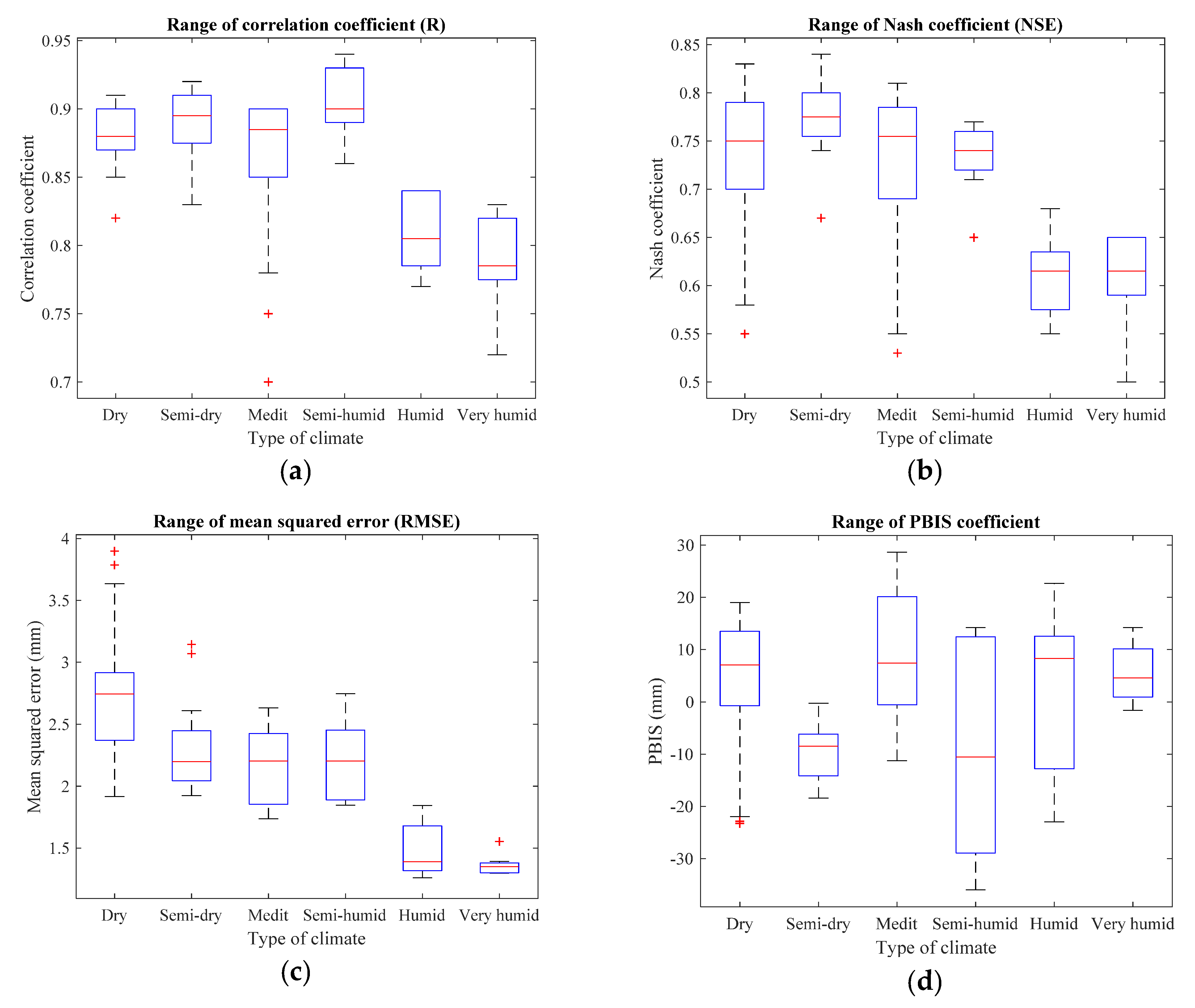
Table 4 shows the range of statistical indicators obtained in validation of the two methods using the two-parameter input combination for the 32 synoptic weather stations in Iran, while
Figure 9 shows box plots of the statistical coefficient values (r, NSE, RMSE, PBIAS). In this case, r was >0.87, NSE > 0.75, RMSE < 2.75 mm, and PBIAS < 10% for the dry, semi-dry, Mediterranean, and semi-humid climate types, while the corresponding values for the humid and very humid climate types were >0.78, >0.62, <1.75 mm, and <9%, respectively. These results confirm the ability of both our methods to simulate pan evaporation for the different climate types in Iran, supporting other findings (first method: two graphs in
Figure 7; second method: Equation (12) with the six climatic correction coefficients in
Table 3).
5. Discussion
Based on the statistical coefficients obtained for the three experimental relationships (linear, quadratic, cubic) in the first method, the quadratic relationship showed the best performance under all climatic conditions. This derived from the better ability of the quadratic relationship to simulate high evaporation than the linear relationship and its better ability to simulate low evaporation than the cubic relationship. The statistical coefficients for the quadratic relationship showed that there was little difference between the values of simulated evaporation for the two- and four-parameter input combinations tested. Therefore, it is not economical to use the four-parameter combination, which includes temperature, relative humidity, sundial, and wind speed, since using a combination of temperature and relative humidity is sufficient to simulate pan evaporation. Examination of the weights obtained for the quadratic relationships for the six climate types in Iran showed that the relationships fell into two groups, representing four (dry, semi-dry, semi-humid, and Mediterranean) and two (humid and very humid) climate types. Therefore, to simplify this method with the two-parameter input combination, graphs were prepared for these two groups with relative humidity and temperature on the axes and pan evaporation drawn as contours.
The statistical coefficients obtained for the six experimental relationships in the first method indicated that the experimental relationship for semi-dry climatic conditions had the greatest ability to simulate pan evaporation. Therefore it was chosen as the basic relationship in the second method. The climatic correction coefficients of this basic relationship determined for other climate types ranged between 0.8 and 1 for the dry, semi-dry, semi-humid, and Mediterranean climate types, and between 0.4 and 0.6 for the humid and very-humid climate types. The significant difference between the range of values show that one single experimental relationship cannot be used for all different climatic conditions using the specific input data. Based on this finding, all experimental relationships presented in previous studies Alazard et al. [
9]; Armstrong et al. [
10]; Delclaux et al. [
60]; Filimonova and Trubetskova [
23]; Granger and Gray [
61]; Linacre [
36]; Samoilenko [
37] need to be revised for use in different climatic conditions, and climatic correction coefficients need to be determined.
A review of previous studies modeling pan evaporation using neural networks and neural fuzzy systems showed that the reported correlation coefficient (r) was between 0.67 and 0.91 [
42,
62,
63,
64,
65]. In contrast, the values obtained for the two methods developed in this study for 38 synoptic weather stations in Iran lay between 0.6 and 0.9. Only one MLP-NN neuron with a simple activation function (y = x) was used in this study, yet there was little difference in the range of r values obtained for the two simple methods developed, and for neural networks and fuzzy neural systems in previous studies. Therefore, use of complex relationships will not necessarily improve performance in simulating pan evaporation and is not economical.
6. Conclusions
Access to a comprehensive but simple method for simulating pan evaporation can play a significant role in estimating the water balance of basins, designing and managing irrigation systems, and managing water resources. In this study, we developed two simple and practical methods for simulating pan evaporation under the six types of climatic conditions found in Iran. In the first method, six experimental relationships (linear, quadratic, and cubic, with two- and four-parameter input combinations) were determined for each climate type in Iran, inspired by the MLP-NN neuron approach and the genetic algorithm optimization model. From these, the best relationship for each climate type was selected and used in the second method as the basic relationship, together with climatic correction coefficients () determined for other climate types using the genetic algorithm optimization model. The accuracy of the two methods was tested using data from 32 synoptic weather stations throughout Iran.
In the first method, statistical evaluations showed that a quadratic relationship had the greatest ability to simulate pan evaporation for the six different climate types, owing to its better ability to simulate higher evaporation than the linear relationship and to simulate lower evaporation than the cubic relationship. Examination of the quadratic relationships obtained for the six climate types showed that those for dry, semi-dry, Mediterranean, and semi-humid climate types were similar, but differed from those for humid and very humid climate types (which were similar to each other). Therefore, two graphs were created for these two groups of climate types, with the horizontal and vertical axis showing temperature and relative humidity, respectively, and with average pan evaporation drawn as a contour.
In the second method, statistical evaluations showed that the quadratic relationship for the semi-dry climate type performed best, so it was used as the basic experimental relationship for the six climate conditions. The values of climatic correction coefficients obtained with this relationship ranged between 0.8 and 1 for the dry, semi-dry, Mediterranean, and semi-humid climate types, and between 0.4 and 0.6 for the humid and very humid climate types.
Both methods for estimating pan evaporation were verified by simulating pan evaporation at 32 synoptic weather stations throughout Iran, which gave NSE values >70%, correlation coefficient (r) >80%, and PBIAS <20%. Two input combinations (with four and two parameters, respectively) were applied for the 32 synoptic weather stations and the statistical coefficients obtained showed no significant differences between these for either of the two new methods. Therefore, using the four-parameter input combination (temperature, relative humidity, sunshine and wind speed) was not economical, as the two-parameter input combination (temperature, relative humidity) performed equally well.
The two new methods presented have some advantages over existing methods, e.g., they consider the six climate types in Iran and a wide area was covered by the data. Thus both methods can simulate pan evaporation for all climate types in Iran, but other methods are not applicable for all climatic conditions. Both methods are also simpler to use than existing methods and the only inputs required are temperature and relative humidity data, which are available for all weather stations in Iran.
Supplementary Materials
The following are available online at
https://www.mdpi.com/article/10.3390/w13202814/s1, Figure S1: Time series of observed and simulated pan evaporation using linear, quadratic, and cubic experimental relationships and both input combinations (2020–2000) for: (a) Shahroud station (semi-dry, two-parameter input combination), (b) Shahroud station (semi-dry, four-parameter input combination), (c) Yasuj station (semi-humid, two-parameter input combination), (d) Yasuj station (semi-humid, four-parameter input combination), (e) Kermanshah station (Mediterranean, two-parameter input combination), (f) Kermanshah station (Mediterranean, four-parameter input combination), (g) Sari station (humid, two-parameter input combination), (h) Sari station (humid, four-parameter input combination). Figure S2: Error tolerance of linear, quadratic, and cubic experimental relationships in estimating pan evaporation (2020–2000) at: (a) Shahroud station (semi-dry, two-parameter input combination), (b) Shahroud station (semi-dry, four-parameter input combination), (c) Yasuj station (semi-humid, two-parameter input combination), (d) Yasuj station (semi-humid, four-parameter input combination), (e) Kermanshah station (Mediterranean, two-parameter input combination), (f) Kermanshah station (Mediterranean, four-parameter input combination), (g) Sari station (humid, two-parameter input combination) (h) Sari station (humid, four-parameter input combination), (i) Rasht station (very humid, two-parameter input combination), (k) Rasht station (very humid, four-parameter input combination). Figure S3: Time series of observed and simulated evaporation using the basic relationship with the six climate correction coefficients (2020–2000) for: (a) Shahroud station (semi-dry, two-parameter input combination), (b) Shahroud station (semi-dry, four-parameter input combination), (c) Yasuj station (semi-humid, two-parameter input combination), (d) Yasuj station (semi-humid, four-parameter input combination), (e) Kermanshah station (Mediterranean, two-parameter input combination), (f) Kermanshah station (Mediterranean, four-parameter input combination), (g) Sari station (humid, two-parameter input combination), (h) Sari station (humid, four-parameter input combination). Table S1: Experimental relationships used in the literature to simulate evaporation from open water surfaces. Table S2: Results of previous studies on sensitive input parameters in simulating pan evaporation. Table S3: Results of previous studies on simulating pan evaporation using MLP-NN. Table S4: Location of synoptic stations in Iran from which data were obtained for the present study. Table S5: Values of statistical coefficients obtained in comparisons between observed pan evaporation and pan evaporation simulated using linear, quadratic, and cubic experimental relationships (2000–2020). The yellow shading indicates the best experimental relationship in each input combination for the six stations. Table S6: Weights of linear, quadratic, and cubic experimental relationships obtained using the genetic algorithm for the six climate types with the two-parameter and four-parameter input combinations. Table S7: Statistical coefficients obtained for comparisons between observed pan evaporation and pan evaporation simulated using correction coefficients (
) and the basic relationship for six selected stations representing different climate conditions and both input combinations. Table S8: Statistical coefficients obtained for comparisons between observed pan evaporation and pan evaporation simulated using the best experimental relationships in the validation step (2000–2020). Table S9: Statistical coefficients obtained for comparisons between observed pan evaporation and pan evaporation simulated using the basic relationship and correction coefficients (
) in the validation step (2000–2020).
Author Contributions
Conceptualization, M.H.D.; Data curation, H.G.; Formal analysis, H.G. and A.H.D.; Investigation, Z.K.; Methodology, M.H.D., H.K. and H.G.; Software, M.H.D. and H.G.; Supervision, H.K., Z.K. and A.H.D.; Visualization, M.H.D. and A.H.D.; Writing—original draft, M.H.D. and H.G.; Writing—review & editing, H.K., Z.K. and A.H.D. All authors have read and agreed to the published version of the manuscript.
Funding
This research did not receive any specific grant from funding agencies in the public, commercial, or not-for-profit sectors.
Institutional Review Board Statement
Not applicable.
Informed Consent Statement
Not applicable.
Data Availability Statement
The data presented in this study is available on request from the corresponding author.
Conflicts of Interest
The authors declare no conflict of interest.
References and Note
- Abtew, W.; Melesse, A. Evaporation and Evapotranspiration; Springer: Dordrecht, The Netherlands, 2013; ISBN 978-94-007-4736-4. [Google Scholar]
- Dehghanipour, A.H.; Moshir Panahi, D.; Mousavi, H.; Kalantari, Z.; Tajrishy, M. Effects of Water Level Decline in Lake Urmia, Iran, on Local Climate Conditions. Water 2020, 12, 2153. [Google Scholar] [CrossRef]
- Ghazvinian, H.; Farzin, S.; Karami, H.; Mousavi, S.F. Investigating the Effect of using Polystyrene sheets on Evaporation Reduction from Water-storage Reservoirs in Arid and Semiarid Regions (Case study: Semnan city). J. Water Sustain. Dev. 2020, 7, 45–52. [Google Scholar] [CrossRef]
- Ghazvinian, H.; Mousavi, S.-F.; Karami, H.; Farzin, S.; Ehteram, M.; Hossain, M.S.; Fai, C.M.; Hashim, H.B.; Singh, V.P.; Ros, F.C.; et al. Integrated support vector regression and an improved particle swarm optimization-based model for solar radiation prediction. PLoS One 2019, 14, e0217634. [Google Scholar] [CrossRef] [PubMed]
- Majhi, B.; Naidu, D.; Mishra, A.P.; Satapathy, S.C. Improved prediction of daily pan evaporation using Deep-LSTM model. Neural Comput. Appl. 2020, 32, 7823–7838. [Google Scholar] [CrossRef]
- Tabari, H.; Marofi, S.; Sabziparvar, A.-A. Estimation of daily pan evaporation using artificial neural network and multivariate non-linear regression. Irrig. Sci. 2010, 28, 399–406. [Google Scholar] [CrossRef]
- Zounemat-Kermani, M.; Kisi, O.; Piri, J.; Mahdavi-Meymand, A. Assessment of Artificial Intelligence–Based Models and Metaheuristic Algorithms in Modeling Evaporation. J. Hydrol. Eng. 2019, 24, 04019033. [Google Scholar] [CrossRef]
- Irmak, S.; Haman, D.Z.; Jones, J.W. Evaluation of Class A Pan Coefficients for Estimating Reference Evapotranspiration in Humid Location. J. Irrig. Drain. Eng. 2002, 128, 153–159. [Google Scholar] [CrossRef]
- Alazard, M.; Leduc, C.; Travi, Y.; Boulet, G.; Salem, A. Ben Estimating evaporation in semi-arid areas facing data scarcity: Example of the El Haouareb dam (Merguellil catchment, Central Tunisia). J. Hydrol. Reg. Stud. 2015, 3, 265–284. [Google Scholar] [CrossRef] [Green Version]
- Armstrong, R.N.; Pomeroy, J.W.; Martz, L.W. Spatial variability of mean daily estimates of actual evaporation from remotely sensed imagery and surface reference data. Hydrol. Earth Syst. Sci. 2019, 23, 4891–4907. [Google Scholar] [CrossRef] [Green Version]
- Meyer, A.F. Evaporation from lakes and reservoirs. A Study on Fifth Years’ Weather Bureau Records; Bulletin of Minnesota Resources Commission: St. Paul, MN, USA, 1942. [Google Scholar]
- Harbeck, G.E. The Lake Hefner water loss investigations. Assoc. Intern. Hydrol. Sci. Publ 1958, 3, 437–443. [Google Scholar]
- Marciano, J.K.; Harbeck, G.E. Mass transfer studies in water loss investigation: Lake Hefner studies. Geological Circular 229; US Geological Survey: Washington, DC, USA, 1952.
- Kim, S.; Kim, H.S. Neural networks and genetic algorithm approach for nonlinear evaporation and evapotranspiration modeling. J. Hydrol. 2008, 351, 299–317. [Google Scholar] [CrossRef]
- Guven, A.; Kişi, Ö. Daily pan evaporation modeling using linear genetic programming technique. Irrig. Sci. 2011, 29, 135–145. [Google Scholar] [CrossRef]
- Benzaghta, M.A.; Mohammed, T.A.; Ghazali, A.H.; Soom, M.A.M. Validation of selected models for evaporation estimation from reservoirs located in arid and semi-arid regions. Arab. J. Sci. Eng. 2012, 37, 521–534. [Google Scholar] [CrossRef]
- Izady, A.; Abdalla, O.; Sadeghi, M.; Majidi, M.; Karimi, A.; Chen, M. A novel approach to modeling wastewater evaporation based on dimensional analysis. Water Resour. Manag. 2016, 30, 2801–2814. [Google Scholar] [CrossRef]
- Eray, O.; Mert, C.; Kisi, O. Comparison of multi-gene genetic programming and dynamic evolving neural-fuzzy inference system in modeling pan evaporation. Hydrol. Res. 2018, 49, 1221–1233. [Google Scholar] [CrossRef]
- Hernández-Pérez, E.; Levresse, G.; Carrera-Hernández, J.; García-Martínez, R. Short term evaporation estimation in a natural semiarid environment: New perspective of the Craig–Gordon isotopic model. J. Hydrol. 2020, 587, 124926. [Google Scholar] [CrossRef]
- Althoff, D.; Filgueiras, R.; Rodrigues, L.N. Estimating Small Reservoir Evaporation Using Machine Learning Models for the Brazilian Savannah. J. Hydrol. Eng. 2020, 25, 5020019. [Google Scholar] [CrossRef]
- Shaw, E.M.; Beven, K.J.; Chappell, N.A.; Lamb, R. Hydrology in practice; CRC press: London, UK, 2010; ISBN 0203030230. [Google Scholar]
- Kokya, B.A.; Kokya, T.A. Proposing a formula for evaporation measurement from salt water resources. Hydrol. Process. 2008, 22, 2005–2012. [Google Scholar] [CrossRef]
- Filimonova, M.; Trubetskova, M. Calculation of evaporation from the Caspian Sea surface. In Proceedings of the 9th ISSH SEMINAR on Stochastic Hydraulics, De Vereeniging, Nijmegen, The Netherlands, 23–24 May 2005. [Google Scholar]
- Poormohammadi, S.; Malekinezhad, H.; Rahimian, M.H. Investigating the role of physiographical factors on temperature-related parameters affecting evapotranspiration (Case study: Yazd province). ARIDBIOM 2010, 1, 9–19. [Google Scholar]
- Patra, K.C. Hydrology and water resources engineering; Alpha Science International: Oxford, UK, 2008; ISBN 1842654217. [Google Scholar]
- Srivastava, A.; Sahoo, B.; Raghuwanshi, N.S.; Singh, R. Evaluation of Variable-Infiltration Capacity Model and MODIS-Terra Satellite-Derived Grid-Scale Evapotranspiration Estimates in a River Basin with Tropical Monsoon-Type Climatology. J. Irrig. Drain. Eng. 2017, 143, 04017028. [Google Scholar] [CrossRef] [Green Version]
- SINGH, V.P.; XU, C.-Y. Evaluation and Generalization of 13 Mass-Transfer Equations for Determining Free Water Evaporation. Hydrol. Process. 1997, 11, 311–323. [Google Scholar] [CrossRef]
- Pandey, P.K.; Nyori, T.; Pandey, V. Estimation of reference evapotranspiration using data driven techniques under limited data conditions. Model. Earth Syst. Environ. 2017, 3, 1449–1461. [Google Scholar] [CrossRef]
- Alsumaiei, A.A. Utility of Artificial Neural Networks in Modeling Pan Evaporation in Hyper-Arid Climates. Water 2020, 12, 1508. [Google Scholar] [CrossRef]
- Malik, A.; Kumar, A.; Kisi, O. Monthly pan-evaporation estimation in Indian central Himalayas using different heuristic approaches and climate based models. Comput. Electron. Agric. 2017, 143, 302–313. [Google Scholar] [CrossRef]
- Martí, P.; González-Altozano, P.; López-Urrea, R.; Mancha, L.A.; Shiri, J. Modeling reference evapotranspiration with calculated targets. Assessment and implications. Agric. Water Manag. 2015, 149, 81–90. [Google Scholar] [CrossRef]
- Tezel, G.; Buyukyildiz, M. Monthly evaporation forecasting using artificial neural networks and support vector machines. Theor. Appl. Climatol. 2016, 124, 69–80. [Google Scholar] [CrossRef]
- Wang, L.; Niu, Z.; Kisi, O.; Li, C.; Yu, D. Pan evaporation modeling using four different heuristic approaches. Comput. Electron. Agric. 2017, 140, 203–213. [Google Scholar] [CrossRef]
- Ashrafzadeh, A.; Malik, A.; Jothiprakash, V.; Ghorbani, M.A.; Biazar, S.M. Estimation of daily pan evaporation using neural networks and meta-heuristic approaches. ISH J. Hydraul. Eng. 2020, 26, 421–429. [Google Scholar] [CrossRef]
- Patle, G.T.; Chettri, M.; Jhajharia, D. Monthly pan evaporation modelling using multiple linear regression and artificial neural network techniques. Water Supply 2020, 20, 800–808. [Google Scholar] [CrossRef]
- Linacre, E.T. Data-sparse estimation of lake evaporation, using a simplified Penman equation. Agric. For. Meteorol. 1993, 64, 237–256. [Google Scholar] [CrossRef]
- Samoilenko, V.S. Sovremennaya teoriya okeanicheskogo ispareniya i ee prakticheskoe primenenie (The Modern Theory of Oceanic Evaporation and its Practical Application). Tr. GOIN 1952, 21, 33. [Google Scholar]
- Ghorbani, M.A.; Deo, R.C.; Yaseen, Z.M.; Kashani, M.H.; Mohammadi, B. Pan evaporation prediction using a hybrid multilayer perceptron-firefly algorithm (MLP-FFA) model: Case study in North Iran. Theor. Appl. Climatol. 2018, 133, 1119–1131. [Google Scholar] [CrossRef]
- Moshir Panahi, D.; Sadeghi Tabas, S.; Kalantari, Z.; Ferreira, C.S.S.; Zahabiyoun, B. Spatio-Temporal Assessment of Global Gridded Evapotranspiration Datasets across Iran. Remote Sens. 2021, 13, 1816. [Google Scholar] [CrossRef]
- Moshir Panahi, D.; Kalantari, Z.; Ghajarnia, N.; Seifollahi-Aghmiuni, S.; Destouni, G. Variability and change in the hydro-climate and water resources of Iran over a recent 30-year period. Sci. Rep. 2020, 10, 7450. [Google Scholar] [CrossRef]
- Soroush, F.; Fathian, F.; Khabisi, F.S.H.; Kahya, E. Trends in pan evaporation and climate variables in Iran. Theor. Appl. Climatol. 2020, 142, 407–432. [Google Scholar] [CrossRef]
- Seifi, A.; Soroush, F. Pan evaporation estimation and derivation of explicit optimized equations by novel hybrid meta-heuristic ANN based methods in different climates of Iran. Comput. Electron. Agric. 2020, 173, 105418. [Google Scholar] [CrossRef]
- Ghazvinian, H.; Bahrami, H.; Ghazvinian, H.; Heddam, S. Simulation of Monthly Precipitation in Semnan City Using ANN Artificial Intelligence Model. J. Soft Comput. Civ. Eng. 2020, 4, 36–46. [Google Scholar] [CrossRef]
- Raziei, T.; Daneshkar Arasteh, P.; Saghafian, B. Annual Rainfall Trend Analysis in Arid and Semi-arid Regions of Central and Eastern Iran. J. Water Wastewater; Ab va Fazilab ( persian ) 2005, 16, 73–81. [Google Scholar]
- Doostan, R.; Alijani, B. Atmospheric Pressure Indices and Climate of Iran. Geogr. Dev. Iran. J. 2016, 14, 67–92. [Google Scholar] [CrossRef]
- Doostkamian, M.; Haghighi, E.; Bourbouri, R. Analyzing and IdentifyingRegional Changes of Hot and Cold Zonesin Iran indifferent Periods. J. Geogr. Environ. Hazards 2017, 6, 141–162. [Google Scholar] [CrossRef]
- Karami, H.; Ghazvinian, H.; Dehghanipour, M.; Ferdosian, M. Investigating the Performance of Neural Network Based Group Method of Data Handling to Pan’s Daily Evaporation Estimation (Case Study: Garmsar City). J. Soft Comput. Civ. Eng. 2021, 1–18. [Google Scholar] [CrossRef]
- Ghazvinian, H.; Karami, H.; Farzin, S.; Mousavi, S.F. Experimental Study of Evaporation Reduction Using Polystyrene Coating, Wood and Wax and its Estimation by Intelligent Algorithms. Irrig. Water Eng. 2020, 11, 147–165. [Google Scholar] [CrossRef]
- Ghazvinian, H.; Karami, H.; Farzin, S.; Mousavi, S.F. Effect of MDF-Cover for Water Reservoir Evaporation Reduction, Experimental, and Soft Computing Approaches. J. Soft Comput. Civ. Eng. 2020, 4, 98–110. [Google Scholar] [CrossRef]
- Hatefi, A.; mosaedi, A.; Jabbbari Nooghabi, M. The role of evapotranspiration in meteorological drought monitoring in some climatic regions of the country. J. Water Soil Conserv. 2016, 23, 1–21. [Google Scholar] [CrossRef]
- Dehghanipour, A.H.; Schoups, G.; Zahabiyoun, B.; Babazadeh, H. Meeting agricultural and environmental water demand in endorheic irrigated river basins: A simulation-optimization approach applied to the Urmia Lake basin in Iran. Agric. Water Manag. 2020, 241, 106353. [Google Scholar] [CrossRef]
- Dehghanipour, A.H.; Zahabiyoun, B.; Schoups, G.; Babazadeh, H. A WEAP-MODFLOW surface water-groundwater model for the irrigated Miyandoab plain, Urmia lake basin, Iran: Multi-objective calibration and quantification of historical drought impacts. Agric. Water Manag. 2019, 223, 105704. [Google Scholar] [CrossRef]
- Ehteram, M.; Mousavi, S.F.; Karami, H.; Farzin, S.; Singh, V.P.; Chau, K.; El-Shafie, A. Reservoir operation based on evolutionary algorithms and multi-criteria decision-making under climate change and uncertainty. J. Hydroinformatics 2018, 20, 332–355. [Google Scholar] [CrossRef]
- Goldberg, D.E. Genetic Algorithms in Search, Optimization & Machine Learning; Addison-Wesley Longman Publishing Co., Inc.: Boston, MA, USA, 1989; ISBN 978-0-201-15767-3. [Google Scholar]
- Goldberg, D.E. Genetic Algorithms: A Bibliography David E. Goldberg, Kelsey Milman, and Christina Tidd Department of General Engineering University of Illinois at Urbana-Champaign Urbana, IL 61801. 1992. [Google Scholar]
- Ho-Huu, V.; Nguyen-Thoi, T.; Truong-Khac, T.; Le-Anh, L.; Vo-Duy, T. An improved differential evolution based on roulette wheel selection for shape and size optimization of truss structures with frequency constraints. Neural Comput. Appl. 2018, 29, 167–185. [Google Scholar] [CrossRef]
- Sharma, D.; Singh, V.; Sharma, C. GA Based Scheduling of FMS Using Roulette Wheel Selection Process. In Proceedings of the International Conference on Soft Computing for Problem Solving (SocProS 2011), Roorkee, India, 20–22 December 2011; Springer: New Delhi, India, 2012; pp. 931–940. [Google Scholar]
- Nash, J.E.; Sutcliffe, J.V. River flow forecasting through conceptual models part I—A discussion of principles. J. Hydrol. 1970, 10, 282–290. [Google Scholar] [CrossRef]
- Yapo, P.O.; Gupta, H.V.; Sorooshian, S. Automatic calibration of conceptual rainfall-runoff models: Sensitivity to calibration data. J. Hydrol. 1996, 181, 23–48. [Google Scholar] [CrossRef]
- Delclaux, F.; Coudrain, A.; Condom, T. Evaporation estimation on Lake Titicaca: A synthesis review and modelling. Hydrol. Process. An Int. J. 2007, 21, 1664–1677. [Google Scholar] [CrossRef]
- Granger, R.J.; Gray, D.M. Evaporation from natural nonsaturated surfaces. J. Hydrol. 1989, 111, 21–29. [Google Scholar] [CrossRef]
- Moazenzadeh, R.; Mohammadi, B.; Shamshirband, S.; Chau, K. Coupling a firefly algorithm with support vector regression to predict evaporation in northern Iran. Eng. Appl. Comput. Fluid Mech. 2018, 12, 584–597. [Google Scholar] [CrossRef] [Green Version]
- Nourani, V.; Sayyah Fard, M. Sensitivity analysis of the artificial neural network outputs in simulation of the evaporation process at different climatologic regimes. Adv. Eng. Softw. 2012, 47, 127–146. [Google Scholar] [CrossRef]
- Samadianfard, S.; Hashemi, S.; Izadyar, M. Estimating daily pan evaporation using machine learning methods. Iran. J. Irrig. Drain. 2018, 12, 1004–1015. [Google Scholar]
- Haghighatjo, P.; Mohammadzadeh shahroodi, Z.; Mohammadrezapour, O. Comparison of gene expression programming (GEP) and neuro-fuzzy methods for estimation of pan evaporation (case study: South Khorasan province). J. Soil Water Resour. Conserv. 2017, 6, 107–117. [Google Scholar]
| Publisher’s Note: MDPI stays neutral with regard to jurisdictional claims in published maps and institutional affiliations. |
© 2021 by the authors. Licensee MDPI, Basel, Switzerland. This article is an open access article distributed under the terms and conditions of the Creative Commons Attribution (CC BY) license (https://creativecommons.org/licenses/by/4.0/).


 ,
, 


