Extending the Applicability of the Meyer–Peter and Müller Bed Load Transport Formula

Abstract

The present paper deals with the applicability of the Meyer–Peter and Müller (MPM) bed load transport formula. The performance of the formula is examined on data collected in a particular location of Nestos River in Thrace, Greece, in comparison to a proposed Εnhanced MPM (EMPM) formula and to two typical machine learning methods, namely Random Forests (RF) and Gaussian Processes Regression (GPR). The EMPM contains new adjustment parameters allowing calibration. The EMPM clearly outperforms MPM and, also, it turns out to be quite competitive in comparison to the machine learning schemes. Calibrations are repeated with suitably smoothed measurement data and, in this case, EMPM outperforms MPM, RF and GPR. Data smoothing for the present problem is discussed in view of a special nearest neighbor smoothing process, which is introduced in combination with nonlinear regression.

1. Introduction

Meyer–Peter, Favre and Einstein [1] published a formula in 1934 related to the transport of uniform sediment on a plane bed, while Meyer–Peter and Müller [2,3] published in 1948 and 1949 the definitive formula related to the transport of sediment mixtures with different values of specific gravity. The main characteristic of the Meyer–Peter and Müller (MPM) formula is the distinction of bed roughness due to individual particles from that bed roughness due to bed forms or the distinction of bed resistance due to skin friction from bed resistance due to bed forms. The historical development of the MPM formula is described in detail in Hager and Boes [4]. In this formula, the unit submerged sediment discharge is calculated, and the roughness effect of the channel bottom and walls is taken into account. Wong and Parker [5], by using the same databases of Meyer–Peter and Müller, have suggested two substantially revised forms of the MPM (1948) formula, in which no correction for bed forms is made. According to Wong and Parker [5], the form drag correction of the MPM formula is unnecessary in the context of the plane bed transport data. The amended bed load transport relations of Wong and Parker are valid for lower-regime plane bed equilibrium transport of uniform sediment.

In the formula applied in our study, the unit sediment discharge is calculated, while the channel bottom roughness is distinguished into roughness due to individual particles and roughness due to bed forms.

Herbertson [6] has examined the bed load formula of Meyer–Peter and Müller (1948) as well as other conventional bed load formulas using similitude theory as a common basis of comparison. Especially for wide channels with invariable grain size and ratio of sediment density to water density, Herbertson [6] suggests that the MPM formula is still incomplete in that the depth effect is not included. The final conclusion of Herbertson regarding the MPM formula is cited as: “…the Meyer–Peter and Müller (1948) formula applies only to material rolling or sliding along the bed load and not to material in suspension, however temporarily. The latter condition would limit the formula to the lower regime of transport and presumably the formula will not take account of material transported by saltation”.

Gomez and Church [7] have tested twelve bed load sediment transport formulas for gravel bed channels, among which is the MPM (1948) formula, using four sets of river data and three sets of flume data. On the basis of the tests performed, which were conducted in each case as if no sediment transport information were available for the river, none of the selected formulas and no other formula is capable of generally predicting bed load transport in gravel bed rivers.

Reid et al. [8] assessed the performance of several popular bed load formulas in the Negev Desert, Israel, and found that the Meyer–Peter and Müller [2] and Parker [9] equations performed best, but their analysis considered only one gravel bed river (Barry et al. [10]).

Martin [11] took advantage of ten years of sediment transport and morphologic surveys on the Vedder River, British Columbia, to test the performance of the Meyer–Peter and Müller [2] equation and two variants of the Bagnold equation [12]. The author concluded that the formulas generally under-predicted gravel transport rates [10].

The MPM formula [2] was also tested in comparison with the formulas of Parker [13], Schoklitsch [14] and Recking [15], by means of a field data set of 6319 bed load samples from sand and gravel bed rivers in the USA. The Meyer–Peter and Müller as well as the Parker equations were chosen because they permit a surface-based calculation with limited knowledge of sediment characteristics, and they are widely used [15]. The discrepancy ratio (average percentage of predicted bed load discharge not exceeding a factor of two in relation to the observed bed load discharge) obtained the value of 3% for the MPM formula, which is the lowest value in comparison to the corresponding values of the other three formulas.

López et al. [16] have tested the predictive power of ten bed load formulas against bed load rates for a large, regulated gravel bed river (Ebro River, NE Iberian Peninsula). The bed load MPM formula [2,3] was included in the ten bed load formulas tested. The discrepancy ratio, as it was defined above, was one of the formula’s performance criteria applied. Especially for the MPM formula, the discrepancy ratio obtained the value 3% for the case of using surface bed material.

Overall, the predictive power of the MPM formula was relatively low. The MPM formula [2] belongs to that category of bed load formulas which are based on the assumption of a critical situation characterizing the incipient motion of grains on the bed. According to Meyer–Peter and Müller, the dimensionless critical shear stress amounts to 0.047. The same critical size for rough, turbulent flow, according to Shields [17], amounts to about 0.06. Gessler [18] reported a value of about 0.046 for a 50% probability of grain movement in a rough, turbulent flow. Miller et al. [19] arrived at a similar value of about 0.045 for rough, turbulent flow without consideration of the probability of movement.

Yang [20] suggested a dimensionless unit stream power equation for the computation and prediction of total sediment concentration without using any criterion for incipient motion. This equation was compared with a similar dimensionless unit stream power equation proposed by Yang [21], with the inclusion of criteria for incipient motion. In accordance with the comparison results, both equations are equally accurate in predicting the total sediment concentration in the sand size range. It should be noted that the new equation of Yang [20] is valid for sediment concentration greater than 20 ppm by weight. Both of Yang’s equations were calibrated especially for Nestos River (northeastern Greece) on the basis of available measurements for bed load and suspended load. Regarding the comparison between predicted and measured values of total load transport rate, the values of the statistical criteria used for both equations were very satisfactory, as reported by Avgeris et al. [22].

Several studies have shown that omitting the incipient motion criterion may lead to better results, compared to the existing formulas. For example, Barry et al. [10], on the basis of 2104 bed load transport observations in 24 gravel bed rivers in Idaho (USA), concluded that formulas containing a transport threshold typically exhibit poor performance. Kitsikoudis et al. [23] have employed data-driven techniques, namely artificial neural networks, adaptive-network-based fuzzy inference system and symbolic regression based on genetic programming, for the prediction of bed load transport rates in gravel-bed steep mountainous streams and rivers in Idaho (USA). The derived models generated results superior to those of some of the widely used bed load formulas, without the need to set a threshold for the initiation of motion, and consequently avoid predicting erroneous zero transport rates.

Some previous studies of the authors on the calibration of MPM formula are reported below:

Papalaskaris et al. [24] have attempted to calibrate the MPM formula both manually and on the basis of the least squares method, in terms of roughness coefficient, for two streams in northeastern Greece: Kosynthos River and Kimmeria Torrent. Papalaskaris et al. [25] have also manually calibrated the MPM formula, in terms of roughness coefficient, for Nestos River (northeastern Greece). In a following study, Sidiropoulos et al. [26] have calibrated the same formula for Nestos River by means of a nonlinear optimization of two suitable parameters, while utilizing the average value of the roughness coefficient found by the manual calibration. In all three studies, the comparison between calculations and measurements of bed load transport rate was made on the basis of the following statistical criteria: root mean square error, relative error, efficiency coefficient, linear correlation coefficient, determination coefficient and discrepancy ratio. The values of the above statistical criteria for the case of manual calibration were more satisfactory, compared to the case of nonlinear optimization. However, the manual calibration was carried out on partial measurement sets, while the nonlinear optimization was carried out on the whole measurement set.

In view of the fact that the predictive power of the MPM formula did not reach particularly high levels, the present paper proposes an Enhanced MPM (EMPM) formula, demonstrating that, under suitable calibration, it shows a much better fitness to field data. Moreover, the performance of the enhanced formula is compared to machine learning methods, showing the competitiveness of the semi-empirical formula versus purely data-driven approaches.

One of the adjustment parameters of the formula is the critical shear stress, the value of which has been discussed and re-adjusted by various researchers, as already cited. In line with these investigations and under the data of this study, a zero value of this parameter gave the optimal calibration results.

Calibration of the EMPM formula was also performed on smoothed data, with the prospect of mitigating possible noise of the field measurements. A nearest neighbor smoothing is introduced and applied both in regard to the MPM formula calibration and to typical machine learning methods. In the case of the smoothed data, the performance of the EMPM formula turns out to be superior.

The introduction of machine learning methods into the field of sediment transport modeling brought about new standards in the error metrics of predicted versus measured data, sometimes tending to overshadow physically based and semi-empirical equations. This paper aims at turning attention back to such equations by introducing generalized forms and by establishing competitive and, in the case of smoothing, even better performance versus machine learning methods.

2. Materials and Methods

2.1. Study Area and Data

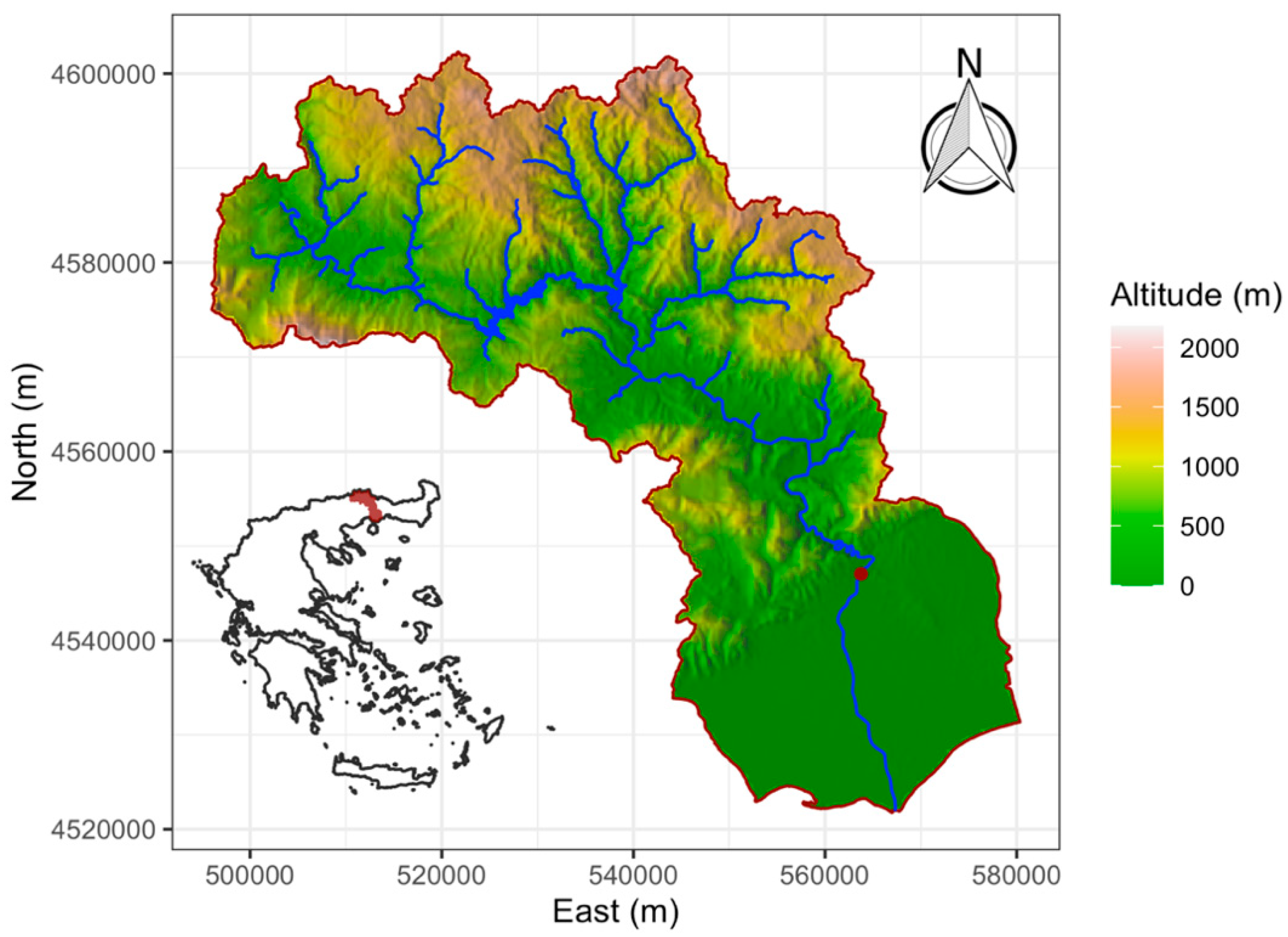
The Nestos River basin (Figure 1, northeastern Greece) considered in this study drains an area of 838 km² and lies downstream of Platanovrysi Dam. The river basin outlet is located at Toxotes. The river basin terrain is covered by forest (48%), bush (20%), cultivated land (24%), urban area (2%) and no significant vegetation (6%). The altitude ranges between 80 m and 1600 m, whereas the length of Nestos River is 55 km. The mean slope of Nestos River in the basin is 0.35%. The stream flow rate and bed load transport rate measurements concerning Nestos River were conducted at a location between the outlet of Nestos River basin (Toxotes) and the river delta. The measurement procedures are described in [25].

The first four statistical moments (mean, standard deviation, skewness and kurtosis) and other statistical properties were used to describe the bed load measured related values (

Table 1. The average statistical properties of bed load related values. SD is an abbreviation for standard deviation.

Variable	Min	Mean	Median	Max	SD	Skew	Kurtosis
${\mathrm{m}}_{\mathrm{Gm}}$ (kg/(s·m))	0	0.0225	0.0175	0.0883	0.0201	1.0790	0.7741
Q (m3/s)	0.100	2.457	1.760	11.020	2.242	1.872	3.393
b (m)	6.00	16.20	15.70	32.00	7.35	0.40	−0.82
h (m)	0.10	0.32	0.31	0.61	0.11	0.33	−0.21
${\mathrm{u}}_{\mathrm{m}}$ (m/s)	0.20	0.47	0.44	1.48	0.21	1.92	5.02
d90 (m)	0.0014	0.0028	0.0030	0.0037	0.0006	−0.8150	−0.2193
d50 (m)	0.0008	0.0045	0.0014	0.0235	0.0064	1.6859	1.0979

).

In concrete terms, m_Gm (kg/(s m)) is the measured bed load transport rate per unit width, Q (m³/s) is the measured stream discharge, b (m) is the measured width of the assumed rectangular cross section, h (m) is the measured flow depth, u_m (m/s) is the measured mean flow velocity, d₅₀ (m) is the median grain diameter of bed load, determined by the granulometric curves, and d₉₀ (m) is a characteristic grain size diameter (in case of taking a stream bed load sample, concerning the sample weight, 90% is composed of grains with size less than or equal to d₉₀).

2.2. Meyer–Peter and Müller (MPM) Bed Load Transport Formula

In the MPM formula, referred to in the introduction, the unit submerged sediment discharge is calculated and the roughness effect of the channel bottom and walls is taken into account.

In the formula, as applied in our study, the unit sediment discharge is calculated while the channel bottom roughness is distinguished into roughness due to individual particles and roughness due to bed forms:

$${\mathrm{m}}_{\mathrm{Gc}}=\frac{8}{\mathrm{g}}\frac{{\mathsf{\rho }}_{\mathrm{F}}}{{\mathsf{\rho }}_{\mathrm{F}}-{\mathsf{\rho }}_{\mathrm{W}}}\sqrt{\frac{1}{{\mathsf{\rho }}_{\mathrm{W}}}}{\left({\mathsf{\tau }}_{\mathrm{o}}-{\mathsf{\tau }}_{\mathrm{o},\mathrm{cr}}\right)}^{3/2}$$

(1)

where:

$${\mathsf{\tau }}_{\mathrm{o}}={\mathsf{\rho }}_{\mathrm{W}}{\mathrm{gI}}_{\mathrm{r}}{\mathrm{R}}_{\mathrm{s}},{\mathsf{\tau }}_{\mathrm{o},\mathrm{cr}}=0.047{{\mathsf{\rho }}^{\prime }\mathsf{\rho }}_{\mathrm{W}}{\mathrm{gd}}_{\mathrm{m}},{\mathsf{\rho }}^{\prime }=\frac{{\mathsf{\rho }}_{\mathrm{F}-}{\mathsf{\rho }}_{\mathrm{W}}}{{\mathsf{\rho }}_{\mathrm{W}}},{\mathrm{I}}_{\mathrm{r}}={(\frac{{\mathrm{k}}_{\mathrm{st}}}{{\mathrm{k}}_{\mathrm{r}}})}^{3/2}\mathrm{I}\mathrm{and}{\mathrm{k}}_{\mathrm{r}}=\frac{26}{\sqrt[6]{{\mathrm{d}}_{90}}}$$

(2)

The symbols of Equations (1) and (2) are explained below:

m_Gc: computed bed load transport rate per unit width (kg/(s·m))

g: gravity acceleration (m/s²)

ρ_F: sediment density (kg/m³)

ρ_w: water density (kg/m³)

τ_o: actual shear stress (N/m²)

τ_o,cr: critical shear stress (N/m²), characterizing the incipient motion of bed grains

I_r: energy line slope due to individual grains

R_s: hydraulic radius of the specific part of the cross section under consideration which affects the bed load transport (m).

d_m: mean diameter of bed load grains (m)

k_st: Strickler coefficient, the value of which depends on the roughness due to individual grains, as well as to stream bed forms (m^1/3/s).

k_r: coefficient, with value depending on the roughness due to individual grain (m^1/3/s)

I: energy line slope due to individual grains and stream bed forms

d₉₀: characteristic grain size diameter (m). It was defined for Table 1.

The basic limitations for the MPM formula are the following:

• Slope of energy line (I) from 0.04% to 2%
• Sediment particle size (d₅₀) from 0.4 mm to 20 mm
• Flow depth (h) from 0.01 m to 1.20 m
• Specific stream discharge (Q/b) from 0.002 m²/s to 2 m²/s
• Relative sediment density (ρ_F/ρ_w) from 0.25 to 3.2
• Particle size > 1 mm, to avoid the effects of apparent cohesion
• Flow depth > 0.05 m, to assure Froude similitude.

At this point, it should be noted that the mean values of the measured energy line slope (longitudinal bed slope in the case of uniform flow), sediment particle size, flow depth, specific stream discharge and relative sediment density are included in the ranges given above.

According to the Einstein–Barbarossa method (e.g., [27])

$$\mathrm{A}={\mathrm{A}}_{\mathrm{s}}+{\mathrm{A}}_{\mathrm{w}}={\mathrm{R}}_{\mathrm{s}}{\mathrm{U}}_{\mathrm{s}}+{\mathrm{R}}_{\mathrm{w}}{\mathrm{U}}_{\mathrm{w}}$$

(3)

where A (m²) is the stream cross section, assuming a rectangular section, approximately, and where R (m) is the hydraulic radius and U (m) is the wetted perimeter. The indices s and w stand for bed and walls, respectively. The hydraulic radius R_w is given by the familiar Manning formula:

$${\mathrm{R}}_{\mathrm{w}}={(\frac{{\mathrm{u}}_{\mathrm{m}}}{{\mathrm{k}}_{\mathrm{w}}{\mathrm{I}}^{0.5}})}^{1.5}$$

(4)

where u_m (m/s) is the mean flow velocity through the cross-sectional area A and k_w (m^1/3/s), a coefficient depending on the roughness of the walls. It is assumed that k_w = k_st. Additionally, I is set equal to the longitudinal stream bed slope on the basis of the assumption of uniform flow.

Then R_s, by combining Equations (3) and (4), turns out as

$${\mathrm{R}}_{\mathrm{s}}=\frac{\mathrm{A}-{\left(\frac{{\mathrm{u}}_{\mathrm{m}}}{{\mathrm{k}}_{\mathrm{w}}{\mathrm{I}}^{0.5}}\right)}^{1.5}{\mathrm{U}}_{\mathrm{w}}}{{\mathrm{U}}_{\mathrm{s}}}$$

(5)

Equation (1) can be converted to a non-dimensional form (see Appendix A):

$${\mathrm{m}}_{\mathrm{Gc}}^{*}=8\left(1+{\mathsf{\rho }}^{\prime }\right){\left[{\left(\frac{{\mathrm{k}}_{\mathrm{st}}}{{\mathrm{k}}_{\mathrm{r}}}\right)}^{3/2}\frac{\mathrm{R}{\mathrm{e}}^{{*}^2}}{{\mathrm{Re}}_{\mathrm{p}50}^2}-0.047\frac{{\mathrm{d}}_{\mathrm{m}}}{{\mathrm{d}}_{50}}\right]}^{3/2}$$

(6)

where

$${\mathrm{m}}_{\mathrm{Gc}}^{*}=\frac{{\mathrm{m}}_{\mathrm{Gc}}}{{\mathsf{\rho }}_{\mathrm{w}}\sqrt{{{\mathsf{\rho }}^{\prime }\mathrm{gd}}_{50}}{\mathrm{d}}_{50}}$$

(7)

$${\mathrm{Re}}_{\mathrm{p}50}=\frac{\sqrt{{{\mathsf{\rho }}^{\prime }\mathrm{gd}}_{50}}{\mathrm{d}}_{50}}{\mathsf{\nu }}$$

(8)

$$\mathrm{R}{\mathrm{e}}^{*}=\frac{\sqrt{{\mathrm{gR}}_{\mathrm{s}}\mathrm{I}}{\mathrm{d}}_{50}}{\mathsf{\nu }}$$

(9)

where ν is the kinematic viscosity of water. The size m_Gc becomes dimensionless by means of Equation (7). The derivation of Equation (9) is given in Appendix A.

Due to the sandy composition of the bed load in the river locations, the mean grain diameter d_m can be approximated by the median grain diameter d₅₀. Therefore, Equation (6) acquires the simpler non-dimensional form:

$${\mathrm{m}}_{\mathrm{Gc}}^{*}=8\left(1+{\mathsf{\rho }}^{\prime }\right){\left[{\left(\frac{{\mathrm{k}}_{\mathrm{st}}}{{\mathrm{k}}_{\mathrm{r}}}\right)}^{3/2}\frac{{\mathrm{Re}}^{*2}}{{\mathrm{Re}}_{\mathrm{p}50}^2}-0.047\right]}^{3/2}$$

(10)

The above non-dimensional scheme is in accordance with the dimensional analysis of Parker and Anderson [28], as utilized in a related paper by Kitsikoudis et al. [23]. Indeed, the non-dimensional groups appearing in Equation (10) are consistent with the dimensionless variables envisaged in the Parker and Anderson analysis. An analogous non-dimensional form has been presented by Wong and Parker [5], attributed originally to N. Chien in a 1954 publication of the US Army Corps of Engineers.

From the non-dimensional form (10), it turns out that, in a way compatible with the dimensional analysis of [28], the following non-dimensional variables determine bed load transport: Re_p50 (Equation (8)), an explicit particle Reynolds number, Re* (Equation (9)), a shear Reynolds number, ρ′ (appearing in the third one of Equations (2)), the submerged specific gravity of the sediment.

2.3. Calibration of an Enhanced Meyer–Peter and Müller (EMPM) Formula

The available data comprise measured values for the physical parameters A, u_m, U_w, U_s and d₅₀, as well as measured values of bed transport rates m_Gm, denoted respectively as A_i, u_mi, U_wi, U_si, d_50,i and m_Gmi, for i = 1, 2,…, N, where N is the number of data points. These subscripted quantities are substituted into the corresponding Equations (7)–(10), giving the non-dimensional bed load transport rate of Equation (10) in terms of measured quantities:

$${\mathrm{m}}_{\mathrm{Gci}}^{*}\left({\mathrm{k}}_{\mathrm{st}}\right)=8\left(1+{\mathsf{\rho }}^{\prime }\right){\left[{\left(\frac{{\mathrm{k}}_{\mathrm{st}}}{{\mathrm{k}}_{\mathrm{ri}}}\right)}^{3/2}\frac{{\mathrm{Re}}_{\mathrm{i}}^{*2}}{{\mathrm{Re}}_{\mathrm{p}50,\mathrm{i}}^2}-0.047\right]}^{3/2}$$

(11)

In Equation (11), k_st emerges as an adjustment parameter. Therefore, the following expression can be used for the calibration of the MPM formula:

$$\mathrm{f}\left({\mathrm{k}}_{\mathrm{st}}\right)={\displaystyle \sum }_{\mathrm{i}=1}^{\mathrm{N}}{\left({\mathrm{m}}_{\mathrm{Gci}}^{*}\left({\mathrm{k}}_{\mathrm{st}}\right)-{\mathrm{m}}_{\mathrm{Gmi}}^{*}\right)}^2$$

(12)

where

$${\mathrm{m}}_{\mathrm{Gmi}}^{*}=\frac{{\mathrm{m}}_{\mathrm{Gmi}}}{{\mathsf{\rho }}_{\mathrm{w}}\sqrt{{{\mathsf{\rho }}^{\prime }\mathrm{gd}}_{50,\mathrm{i}}}{\mathrm{d}}_{50,\mathrm{i}}},\mathrm{i}=1,\dots ,\mathrm{N}$$

(13)

and m_Gmi, i = 1,…,N, denote measured values of bed load transport rate. Calibration with respect to one parameter only, namely k_st, has already been tried (Sidiropoulos et al., 2018). In this paper, Equation (12) is further extended, so as to include more adjustment parameters:

$${\mathrm{m}}_{\mathrm{Gci}}^{*}\left({\mathrm{k}}_{\mathrm{st}},\mathsf{\alpha },\mathsf{\beta },\mathsf{\gamma }\right)=8\mathsf{\alpha }\left(1+{\mathsf{\rho }}^{\prime }\right){\left[{\left(\frac{{\mathrm{k}}_{\mathrm{st}}}{{\mathrm{k}}_{\mathrm{ri}}}\right)}^{\mathsf{\beta }}\frac{{\mathrm{Re}}_{\mathrm{i}}^{*2}}{{\mathrm{Re}}_{\mathrm{p}50,\mathrm{i}}^2}-\mathsf{\gamma }\right]}^{3/2}$$

(14)

Equation (14) will be referred to as the Enhanced Meyer–Peter and Müller (EMPM) formula.

Equation (14) can be written as follows in a generalized form:

$${\mathrm{m}}_{\mathrm{Gci}}^{*}={\mathrm{f}}_{\mathrm{M}}\left(d_{\mathrm{M}};p_{\mathrm{i}}\right)$$

(15)

where d_M = (k_st, α, β, γ) is the vector of parameters,

$$p_{\mathrm{i}}=\left({\mathrm{A}}_{\mathrm{i}},{\mathrm{U}}_{\mathrm{mi}},{\mathrm{U}}_{\mathrm{wi}},{\mathrm{U}}_{\mathrm{si}},{\mathrm{d}}_{50,\mathrm{i}},{\mathrm{k}}_{\mathrm{ri}},{\mathrm{I}}_{\mathrm{i}}\right),\mathrm{i}=1,2,\dots ,\mathrm{N}$$

(16)

is the vector of measured quantities that were suitably grouped in Equation (10), and

$${\mathrm{f}}_{\mathrm{M}}\left(d_{\mathrm{M}};p_{\mathrm{i}}\right)=8\mathsf{\alpha }\left(1+{\mathsf{\rho }}^{\prime }\right){\left[{\left(\frac{{\mathrm{k}}_{\mathrm{st}}}{{\mathrm{k}}_{\mathrm{ri}}}\right)}^{\mathsf{\beta }}\frac{{\mathrm{Re}}_{\mathrm{i}}^{*2}}{{\mathrm{Re}}_{\mathrm{p}50,\mathrm{i}}^2}-\mathsf{\gamma }\right]}^{3/2}$$

(17)

In analogy to Equations (11) and (12), the difference between computed and measured quantities is defined as

$${\mathrm{e}}_{\mathrm{i}\mathrm{M}}={\mathrm{f}}_{\mathrm{M}}\left(d_{\mathrm{M}};p_{\mathrm{i}}\right)-{\mathrm{m}}_{\mathrm{Gmi}}^{*}$$

(18)

where ${\mathrm{m}}_{\mathrm{Gmi}}^{*}$ is given by Equation (13) and f_M by Equation (17).

The objective function of the calibration problem is

$${\mathrm{F}}_{\mathrm{M}}\left(d_{\mathrm{M}}\right)={{\displaystyle \sum }}_{\mathrm{i}=1}^{\mathrm{N}}{\mathrm{e}}_{\mathrm{iM}}^2$$

(19)

where N is the number of measurement points.

The minimization of the objective function F_M of Equation (19) was executed by a genetic algorithm followed by a Nelder–Mead local search.

2.4. Application of Machine Learning Schemes

A common pitfall in the use of machine learning algorithms is the expectation of performance regardless of the nature and limitations of the problem and of the presence of noisy data. In the context of bed load estimation, especially for data that are coming from natural streams, errors are expected to be higher, as testified by the sediment transport literature, in which errors are predominantly reported as ratios and not as differences of compared quantities.

In a preliminary stage of analysis, various machine and statistical learning methods have been evaluated, such as neural networks (various architectures and regularization techniques), support vector regression, decision trees, linear models, K-NN regression, Gaussian Processes Regression (GPR) and Random Forests (RF). Most methods gave similar results with the exception of neural networks, which had a tendency to overfit or, in other words, they fitted too closely on the data, memorizing the noise and, as a result, were unable to adequately generalize on new data.

In the sequel, RF and GPR algorithms are presented so as to have a broader representation of machine learning methods. RF had the best performance and the results obtained regarding their generalization ability in this problem and dataset justify their use, as reported later in Section 3.

2.4.1. Random Forests

Random Forests (RF) is a data-driven algorithm in the area of supervised learning which tries to fit a model using a set of paired input variables and their associated output responses, and can be used in classification and regression problems. In summary, RF consists of a number of decision trees [29]. For each tree, a random set is created from the dataset via bootstrapping [29], and in each node of the tree a random set of n input variables from the p variables of the dataset is considered to pick the best split [29]. The prediction of the output response in regression problems is the mean value of the estimations of these random decision trees. RF is one of the most popular methods applied in machine learning because of: (a) its robustness to outliers and overfitting, (b) its ability to perform feature selection and (c) the fact that its default hyperparameters (i.e., the set of parameters that have to be selected a priori in order to train a RF), as implemented in software, give satisfactory results [30].

The measured data quantities defined above, under the vector p_i, serve as input variables in the RF learning scheme, while ${\mathrm{m}}_{\mathrm{Gmi}}$ will be the corresponding target for the output. The general form of Equations (18) and (19) can be used again for the formation of the objective function, as follows:

Let

$${\mathrm{m}}_{\mathrm{Gci}}^{*}={\mathrm{f}}_{\mathrm{R}}\left(d_{\mathrm{R}};p_{\mathrm{i}}\right)$$

(20)

in analogy to Equation (15), where d_R is the vector of the RF parameters (i.e., the set of decision trees that operate as an ensemble) that will be determined through training.

Then the deviation of measured from computed values is

$${\mathrm{e}}_{\mathrm{iR}}={\mathrm{f}}_{\mathrm{R}}\left(d_{\mathrm{R}};p_{\mathrm{i}}\right)-{\mathrm{m}}_{\mathrm{Gmi}}^{*}$$

(21)

and the objective value of the problem will be

$${\mathrm{F}}_{\mathrm{R}}\left(d_{\mathrm{R}}\right)={{\displaystyle \sum }}_{\mathrm{i}=1}^{\mathrm{N}}{\mathrm{e}}_{\mathrm{iR}}^2$$

(22)

2.4.2. Gaussian Processes Regression

A completely different alternative is Gaussian Processes Regression (GPR), which can be briefly described as follows: In the area of machine learning, Williams and Rasmussen [31] developed a regression algorithm based on Gaussian processes, which is a non-parametric, Bayesian approach that has the ability to work well with small datasets. In the framework of that algorithm, the prediction for an input test point x is derived by means of a Gaussian stochastic process with an assumed mean equal to 0 and with a variance σ² calculated in terms of covariances involving x and the training data. A suitable covariance function is selected and parametrized, and finally, the hyperparameters involved are determined through optimization.

In this case, the formal scheme of Equations (20)–(22) is retained, with d_R replaced by d_G for GPR. The vector d_G represents the internal parameters of the respective machine learning process, which will be optimally determined according to the above outline.

2.5. Training and Testing Procedures

Three methods are presented here for modeling bed load sediment transport. The first one is the calibration of the EMPM formula, while the second and the third consist in the application of RF and GPR machine learning methods respectively. In all three cases, a resampling method needs to be executed in order to estimate the generalization error of the methods or, specifically, the measure of accuracy of the methods to predict outcome values from data that are not known a priori. For that reason, bootstrapping [29] is applied, a procedure that was repeated 100 times.

Every bootstrap sample dataset consists of 116 points generated through random sampling with replacement of the original 116 data points. Consequently, some observations may appear more than once and some not at all. The latter are used to estimate the generalization error (out-of-the-bag error) and the former lead to the training error of the methods.

The simulation will be carried out for the original raw data, first by calibration of the EMPM formula and then by training the RF and GPR machine learning methods. Thereafter, the original data will be subjected to smoothing and the simulation will be repeated for the smoothed data by the same three methods.

2.6. Nearest Neighbor Smoothing

A smoothing process based on nearest neighbors is introduced as follows:

For each vector p_i of input measured quantities (Equation (16)), the distances are computed to all other vectors p_j, j = 1, 2,…, N, where N is the number of available measurement points. The k nearest neighbors to p_i are then picked out and the average of these is taken, as well as the average of the corresponding bed load transport measurements. These averages will replace the original data. The process is formalized as follows:

Let

$${\mathrm{r}}_{\mathrm{i},\mathrm{j}}=||p_{\mathrm{i}}-p_j||,\mathrm{j}=1,2,\dots ,\mathrm{N}$$

(23)

be the distances between p_i and all p_j’s, including p_i itself.

Let

$${\mathrm{D}}_{\mathrm{i}}=\left\{{\mathrm{r}}_{\mathrm{i}1},{\mathrm{r}}_{\mathrm{i}1},\dots ,{\mathrm{r}}_{\mathrm{iN}}\right\}$$

(24)

be the set of the distances of p_i from all other parameter vectors, as computed according to Equation (22).

Let

$${\mathrm{r}}_{\mathrm{i},\mathrm{i}1},{\mathrm{r}}_{\mathrm{i},\mathrm{i}2},\dots .{\mathrm{r}}_{\mathrm{i},\mathrm{ik}}$$

be the k smallest members of the set D_i of Equation (23) and let

$$p_{\mathrm{i}1},p_{\mathrm{i}2},\dots ,p_{\mathrm{ik}}\mathrm{and}{\mathrm{m}}_{\mathrm{Gmi}1}^{*}, {\mathrm{m}}_{\mathrm{Gmi}2}^{*},\dots ,{\mathrm{m}}_{\mathrm{Gmik}}^{*}$$

be the corresponding k vectors and associated bed load measurements expressed in non-dimensional form as above (Equation (13)).

Then the following averaging is performed:

$$p_{\mathrm{i}}^{\mathrm{k}}=\frac{1}{\mathrm{k}}{{\displaystyle \sum }}_{\mathrm{j}=\mathrm{i}}^{\mathrm{k}}{p}_{\mathrm{ij}},\mathrm{i}=1,2,\dots ,\mathrm{N}$$

(25)

$${\mathrm{m}}_{\mathrm{Gmi}}^{*\mathrm{k}}=\frac{1}{\mathrm{k}}{{\displaystyle \sum }}_{\mathrm{j}=\mathrm{i}}^{\mathrm{k}}{\mathrm{m}}_{\mathrm{Gmij}}^{*},\mathrm{i}=1,2,\dots ,\mathrm{N}$$

(26)

The pair $(p_{\mathrm{i}}^{\mathrm{k}},{\mathrm{m}}_{\mathrm{Gmi}}^{*\mathrm{k}}$) will replace the pair $(p_{\mathrm{i}},{\mathrm{m}}_{\mathrm{Gmi}}^{*}$) in Equations (18) and (19) for the formation of objective function F_M, and in Equations (21) and (22) for the formation of objective function F_R.

It needs to be noted here that the nearest neighbor technique is used for smoothing only and not for prediction, as known from the literature (e.g., [29]). Prediction is performed by the nonlinear regression that follows the smoothing.

3. Results and Discussion

3.1. Implementation of Algorithms

The EMPM formula presented in this paper was calibrated with respect to the four parameters k_st, α, β and γ, contained in the objective function of Equation (19). The last parameter γ is related to the so-called threshold referred to in the introduction, which turned out to be zero for our data and for all repetitions of the EMPM formula calibrations. The required minimization was executed by a genetic algorithm followed by a Nelder–Mead local search. As is well-known, the genetic algorithm points to the area within which the minimum needs to be sought and the sequent local search more accurately yields the location of the minimum [32].

The RF and GPR applications are completely independent, pure data-driven processes, as already explained in Section 2.4. They were performed by means of the algorithms provided by the Mathematica Computation System [33], with automatic selection of the optimal hyperparameters.

For the nearest neighbor smoothing, the number of nearest neighbors was chosen equal to k = 5.

3.2. Error Metrics

The error metrics included are RMSE, Mean Discrepancy Ratio (MDR) and coefficient of determination (R²).

The discrepancy ratio for individual measured–calculated quantities is defined as

dr_i = m_Gci/m_Gmi, i = 1, 2,…,N

(27)

where N is the number of measurements.

The Mean Discrepancy Ratio (MDR) is

$$\mathrm{MDR}=\frac{1}{\mathrm{N}}{\displaystyle \sum }_{\mathrm{i}=1}^{\mathrm{N}}{\mathrm{dr}}_{\mathrm{i}}$$

(28)

As already stated in Section 2.5, the process of training and test set formation was repeated 100 times within a bootstrapping scheme, each time obtaining a different set of the adjustment parameters α, β and γ and corresponding values of RMSE.

Table 2. Mean and standard deviation of error metrics for raw data and for the out-of-the-bag dataset from bootstrap resampling. RMSE units: kg/(s·m).

		Mean	SD
RDOF Raw Data Original Formula	RMSE	0.05646	0.00564
	MDR	6.20336	1.44002
	R2	0.16077	0.12808
RDEF Raw Data Enhanced Formula	RMSE	0.01928	0.00217
	MDR	3.06172	0.92239
	R2	0.47922	0.08730
RDRF Raw Data Random Forests	RMSE	0.01832	0.00247
	MDR	3.49139	1.49874
	R2	0.54513	0.10054
RDGP Raw Data Gaussian Processes	RMSE	0.01999	0.00280
	MDR	3.36799	1.82963
	R2	0.34135	0.10937

and

Table 3. Mean and standard deviation of error metrics for smoothed data and for the out-of-the-bag dataset from bootstrap resampling. RMSE units: kg/(s·m).

		Mean	SD
SDOF Smoothed Data Original Formula	RMSE	0.04159	0.006065
	MDR	2.37244	0.719034
	R2	−0.94236	0.235836
SDEF Smoothed Data Enhanced Formula	RMSE	0.00926	0.001925
	MDR	1.20260	0.27857
	R2	0.48299	0.20773
SDRF Smoothed Data Random Forests	RMSE	0.01030	0.002019
	MDR	1.31873	0.344024
	R2	0.40220	0.123037
SDGP Smoothed Data Gaussian Processes	RMSE	0.01180	0.002842
	MDR	1.27084	0.356768
	R2	0.22199	0.172782

give, for each case, the mean value of RMSE over the 100 repetitions, along with the associated standard deviation. The same tables also show the mean values and standard deviations for the 100 repetitions of RMSE, MDR and R².

The comparisons among the employed algorithms will be based mainly on RMSE, which also formed the basis of the objective function. R² is a well-established index in hydrologic modeling, being the same as the well-known Nash–Sutcliff Efficiency index (NSE). However, serious reservations have been reported in the pertinent literature as to its autonomous use for performance evaluation [34]. Various cases have been reported in which a good model could have low R² and a bad model high R². Also, in the context of sediment transport modeling, due to inherent difficulties and due to the noise in field data, low R² values would not be a surprise.

In the same context and for the same reasons, the discrepancy ratio, rather than R², has been a primary realistic index, since it estimates errors in terms of ratios rather than differences between measured and computed values. Regarding discrepancy ratios in this study, a qualitative comparison of the present results to analogous results of the literature will be given in Section 3.4.

3.3. Results of Error Metrics and Related Comparisons

Table 2 covers the various cases based on raw data for EMPM vs. MPM and vs. RF and GPR, while Table 3 covers the corresponding cases for smoothed data. The nomenclature of the various cases is given on the leftmost columns of Table 2 and Table 3.

As expected, the performance of the calibrated EMPM formula is definitely higher in comparison to the original MPM formula. Indeed, it can be seen in Table 2 that, for Raw Data and for the Enhanced MPM Formula (RDEF), the out-of-the-bag test set RMSE mean value for the 100 bootstrapping repetitions is equal to 0.019278, while the corresponding quantity for the Original Formula (RDOF) is equal to 0.056466.

It can be observed from Table 2 and Table 3 that the standard deviations, especially for RMSE, are by an order of magnitude smaller than the mean values. Therefore, the mean error metrics of the tables and, especially, the mean RMSE, are representative.

Although it may not be of particular use at present, indicative sets of parameters can be given and, as such, those are chosen that closely produce the mean RMSE of RDEF and SDEF, respectively. Specifically,

• for RDEF, k_st = 10.7379, α = 0.2000, β = 1.1199, γ = 0 and
• for SDEF, k_st = 30.00, α = 0.6519, β = 3.5374, γ = 0.

While RDEF is superior to RDOF, it is also competitive versus the machine learning methods (RDRF and RDGP), as seen on Table 2. On the other hand, in the cases of smoothed data (Table 3), EMPM (SDEF) outperforms the original formula MPM (SDOF), as well as Random Forests (SDRF) and Gaussian Processes Regression (SDGP). These facts are seen clearly by observing the respective RMSE’s in Table 2 and Table 3, along with the corresponding small standard deviations.

As discussed in Section 3.2, the values of R² are not to be taken as a sole representative measure of performance. In comparative terms, the R² value for RDEF from Table 2 is 0.47962, while for RDOF it is 0.169077; i.e., R² is about three times greater for the enhanced versus the original MPM formula.

The same relative improvement in performance applies to RMSE, and the conclusions drawn from Table 2 can be visualized in Figure 2, which shows the corresponding boxplots.

Similar comparisons can be made for the other cases of Table 2 and Table 3, but the general status of the results is further indicated by the comparison of discrepancy ratios obtained in this study versus analogous quantities of the pertinent literature, as described in the next section.

3.4. Discrepancy Ratio Comparisons

In the context of sediment transport modeling, an established indicator is the discrepancy ratio. It would, therefore, be appropriate to consider characteristic results of this ratio in the pertinent literature and compare them to those of the present study. Indeed, in References [15,16], three indices, D₁, D₂ and D₃, appear in relation to discrepancy ratios:

Let dr_i’s be the ratios defined in Equation (27). Then

• D₁ is defined as the percentage of dr_i’s such that 0.5 ≤ dr_i ≤ 2.
• D₂ is defined as the percentage of dr_i’s such that 0.25 ≤ dr_i ≤ 4.
• D₃ is defined as the percentage of dr_i’s such that 0.1 ≤ dr_i ≤ 10.

In [15], a characteristic set (D₁, D₂, D₃) is equal to (3%, 7%, 9%), especially for the MPM formula resulting from 6319 values of a field dataset regarding sand and gravel bed streams in USA. In [16], D₁ = 3%, especially for the MPM formula applied to Ebro River (Spain) with the gravel bed.

Indicative computed corresponding values in this study are as follows:

• Raw data, original formula: (D₁, D₂, D₃) = (32%, 45%, 60%).
• Raw data, enhanced formula: (D₁, D₂, D₃) = (55%, 81%, 97%).

The above results are not directly comparable to those of [15,16] due to different datasets and validation schemes. However, they render a good indication of a better fitting and of the improvement brought about by the enhanced formula. Discrepancy ratio results in this study are even better for the smoothed data.

3.5. Examination of Possible Overfitting

In order to detect any cases of overfitting, Table 5 lists the RMSE mean values of the bootstrapped training sets versus those of the corresponding out-of-the-bag test sets. The latter are also given in Table 2 and Table 3. It is immediately seen that there is no question of overfitting in the EMPM formula (RDEF and SDEF), while there is an indication of overfitting in the GPR (RDGP and SDGP) due to larger differences between the RMSE mean values of training and test sets. Regarding RF, there is clearly no overfitting in RDRF. In the case of the smoothed data (SDRF), overfitting to a lesser degree versus SDGP is indicated in

Table 4. RMSE mean values of bootstrap training and out-of-the-bag test sets. RMSE units: kg/(s·m).

	Training Set	Test Set
RDOF	0.05427	0.05646
RDEF	0.01785	0.01928
RDRF	0.01367	0.01833
RDGP	0.00690	0.01999
SDOF	0.04476	0.04159
SDEF	0.01037	0.00926
SDRF	0.00696	0.01030
SDGP	0.00191	0.01180

.

Overfitting would not be expected of the EMPM formula, and this fact is verified in the above Table 4, but overfitting is very often not easily avoidable in machine learning methods. The best behavior in this regard was exhibited by RF.

3.6. Statistical Comparisons

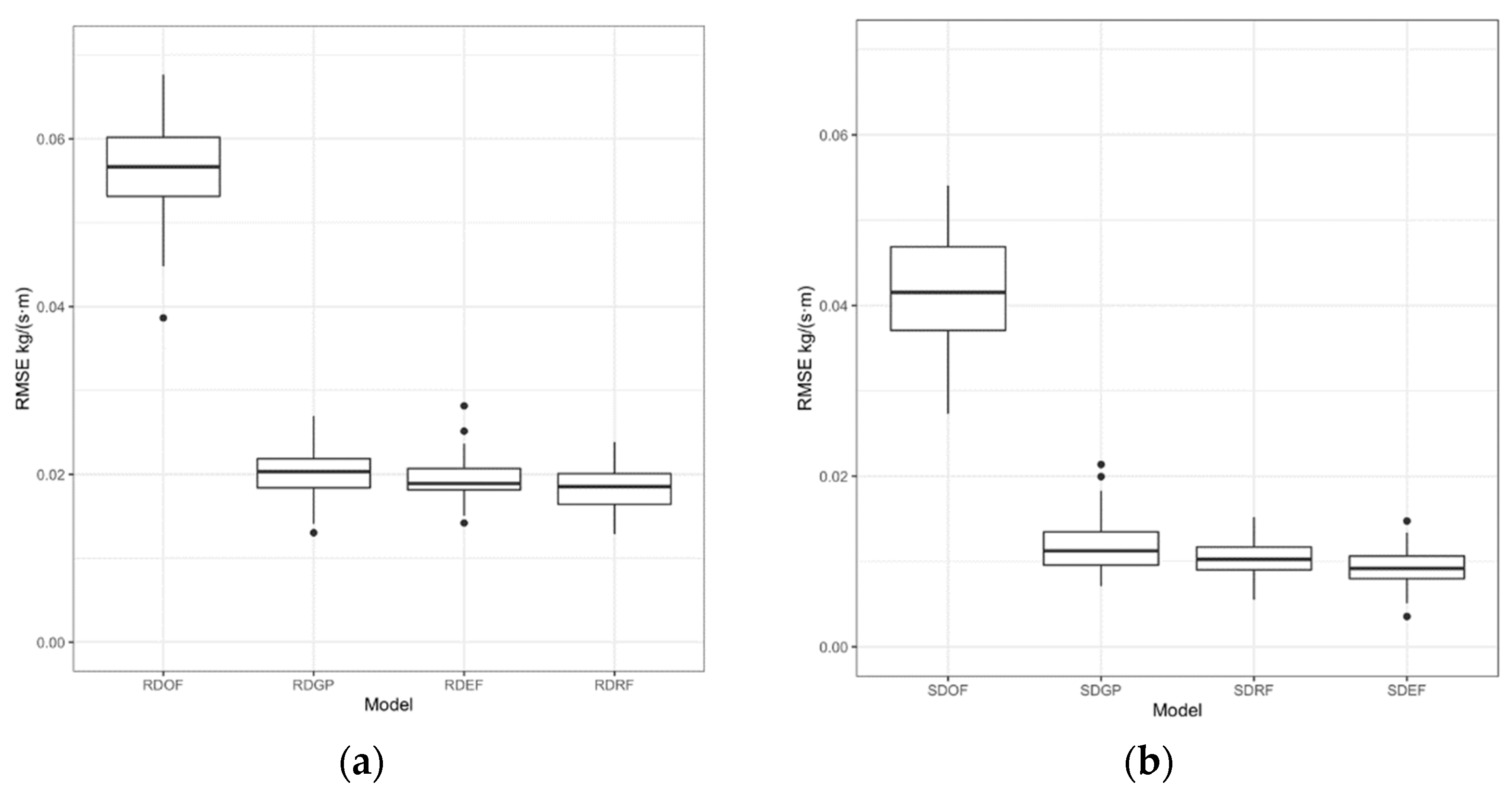
Besides the computation results shown in Table 2 and Table 3 and in Figure 2, statistical comparisons between the methods used are also in order.

The comparison of the algorithms was based on the work of Demšar [35] and García et al. [36] on the use of non-parametric methods for the evaluation of results of machine learning algorithms, because parametric hypothesis testing methods (pairwise t-test and ANOVA) were not deemed suitable due to the nature of the algorithms. The Friedman test [37] was performed in order to determine whether an algorithm has a systematically better or worse performance. The obtained p-values (both < 2.2 × 10⁻¹⁸) indicated that the null hypothesis of all the algorithms performing the same could safely be rejected. Then, post-hoc tests followed for all possible pairs of algorithms using the Wilcoxon signed rank test [38]. Because of the multiple pairwise tests, the p-values that resulted were adjusted using the Benjamini and Hochberg method [39], which controls the false discovery rate (

Table 5. To the right of the diagonal stand the estimated differences of RMSE between models for raw data. To the left of the diagonal stand the adjusted p-values for the H₀ (null hypothesis): difference = 0.

	RDOF	RDGP	RDEF	RDRF
RDOF	-	0.0363	0.0377	0.0381
RDGP	7.9 × 10−18	-	0.0014	0.0017
RDEF	7.9 × 10−18	0.02	-	0.0003
RDRF	7.9 × 10−18	4.3 × 10−5	0.01	-

and

Table 6. To the right of the diagonal stand the estimated differences of RMSE between models for smoothed data. To the left of the diagonal stand the adjusted p-values for the H₀ (null hypothesis): difference = 0.

	SDOF	SDGP	SDRF	SDEF
SDOF	-	0.0303	0.0313	0.0323
SDGP	7.9 × 10−18	-	0.0010	0.0020
SDRF	7.9 × 10−18	8.2 × 10−4	-	0.0010
SDEF	7.9 × 10−18	7.6 × 10−9	5.3·10−4	-

). Table 5 shows the adjusted p-values below the main diagonal and at the upper diagonal positions, showing the estimated differences between methods. Table 6 shows the corresponding quantities for smoothed data. Indeed, the p-values indicate statistical differences, and it is noted that the enhanced formula not only shows better performance compared to the original formula, but also compared to the machine learning methods.

3.7. Indicative Scatter Plots

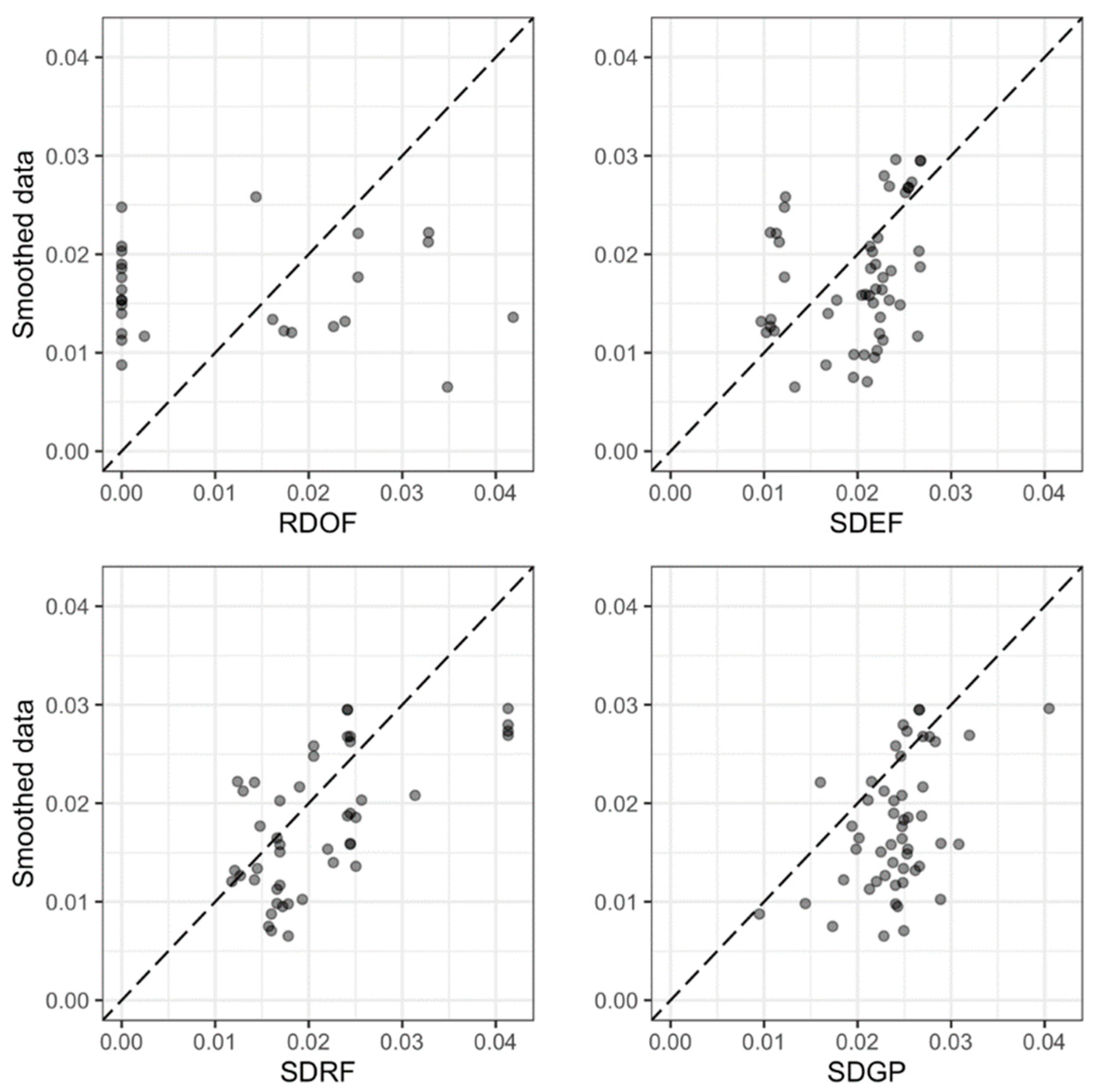
Figure 3 shows indicative scatter plots of predicted versus measured values for a random out-of-the-bag dataset for observed bed load measurement values (kg/(s·m)), and Figure 4 shows corresponding plots for smoothed data. It can visually be verified that the enhanced formula and both machine learning methods exhibit superior performance compared to the initial MPM formula, consistent with the mean error metrics of Table 2 and Table 3.

4. Conclusions

The advent of machine learning methods has also contributed to progress in the area of sediment transport modeling. Purely data-driven methods that appeared in the literature were found to outperform well-known physically based and semi-empirical equations. In an effort to enhance the performance of such equations, the Meyer–Peter and Müller bed load transport formula is extended in the present paper by the addition of suitable adjustment parameters, for the purpose of reinforcing its predictive abilities.

The resulting Enhanced Meyer–Peter and Müller formula presented a definitely improved performance in comparison to the original formula, one which is also competitive to purely data-driven techniques and even superior in the case of smoothed data. As a characteristic data-driven technique, the Random Forests learning scheme was chosen, due to its advantages in terms of robustness against outliers and overfitting, considering the noise contained in the field data of this study. A completely different machine learning method, Gaussian Processes Regression, was also tried and gave similar results, but was found to overfit on the training data.

For the purpose of countering noise effects, data smoothing is important and needs to be further considered for problems involving sediment transport field data, such as the present one. A nearest neighbor data smoothing process is presented and combined with nonlinear regression, a scheme different from the well-known nearest neighbor regression of the literature. Under smoothing, the enhanced MPM formula shows better performance, even compared to the machine learning methods.

The methods presented in this paper call for further applications in other natural streams with values of the variables beyond the range of boundary values given in the present article, as well as in modeling with laboratory data. Additionally, further research would be useful in the direction of hybrids involving both machine learning and sediment transport formulas.

References

- Meyer-Peter, E.; Favre, H.; Einstein, A. Neuere Versuchsresultate über den Geschiebetrieb. Schweiz. Bauztg. 1934, 103, 147–150. [Google Scholar]
- Meyer-Peter, E.; Müller, R. Formulas for bed-load transport. In Proceedings of the 2nd IAHR Congress, Stockholm, Sweden, 7–9 June 1948; IAHR: Delft, The Netherlands, 1948; Volume A2, pp. 1–26. [Google Scholar]
- Meyer-Peter, E.; Müller, R. Eine Formel zur Berechnung des Geschiebetriebs. Schweiz. Bauztg. 1949, 67, 29–32. [Google Scholar]
- Hager, W.H.; Boes, R.M. Eugen Meyer-Peter and the MPM sediment transport formula. J. Hydraul. Eng. 2018, 144, 02518001. [Google Scholar] [CrossRef]
- Wong, M.; Parker, G. Reanalysis and correction of bed-load relation of Meyer-Peter and Müller using their own database. J. Hydraul. Eng. 2006, 112, 1159–1168. [Google Scholar] [CrossRef] [Green Version]
- Herbertson, J.G. A critical review of conventional bed load formulae. J. Hydrol. 1969, 8, 1–26. [Google Scholar] [CrossRef]
- Gomez, B.; Church, M. An assessment of bed load sediment transport formulae for gravel bed rivers. Water Resour. Res. 1989, 25, 1161–1186. [Google Scholar] [CrossRef]
- Reid, I.; Powell, D.M.; Laronne, J.B. Prediction of bed-load transport by desert flash floods. J. Hydraul. Eng. 1996, 122, 170–173. [Google Scholar] [CrossRef]
- Parker, G. Surface-based bed load transport relation for gravel rivers. J. Hydraul. Res. 1990, 28, 417–436. [Google Scholar] [CrossRef]
- Barry, J.J.; Buffington, J.M.; King, J.G. A general power equation for predicting bed load transport rates in gravel bed rivers. Water Resour. Res. 2004, 40, W10401. [Google Scholar] [CrossRef]
- Martin, Y. Evaluation of bed load transport formulae using field evidence from the Vedder River, British Columbia. Geomorphology 2003, 53, 73–95. [Google Scholar] [CrossRef]
- Bagnold, R.A. An empirical correlation of bed load transport rates in flumes and natural rivers. Proc. R. Soc. Lond. 1980, 372, 453–473. [Google Scholar]
- Parker, G. Hydraulic geometry of active gravel rivers. J. Hydraul. Div. 1979, 105, 1185–1201. [Google Scholar] [CrossRef]
- Schoklitsch, A. Handbuch des Wasserbaus, 3rd ed.; Springer: Wien, Austria, 1962. [Google Scholar]
- Recking, A. A comparison between flume and field bed load transport data and consequences for surface-based bed load transport prediction. Water Resour. Res. 2010, 46, W03518. [Google Scholar] [CrossRef] [Green Version]
- López, R.; Vericat, D.; Batalla, R.J. Evaluation of bed load transport formulae in a large regulated gravel bed river: The lower Ebro (NE Iberian Peninsula). J. Hydrol. 2014, 510, 164–181. [Google Scholar] [CrossRef] [Green Version]
- Shields, A. Anwendung der Ähnlichkeitsmechanik und der Turbulenzforschung auf die Geschiebebewegung; Mitteilungen der Preussischen Versuchsanstalt für Wasser-und Schiffbau, Heft 26; Berlin, Germany, 1936. [Google Scholar]
- Gessler, J. Beginning and ceasing of sediment motion. In River Mechanics; Shen, H.W.: Fort Collins, CO, USA, 1971. [Google Scholar]
- Miller, M.C.; McCave, I.N.; Komar, P.D. Threshold of sediment motion under unidirectional currents. Sedimentology 1977, 24, 507–527. [Google Scholar] [CrossRef]
- Yang, C.T. Unit stream power equation for total load. J. Hydrol. 1979, 40, 123–138. [Google Scholar] [CrossRef]
- Yang, C.T. Incipient motion and sediment transport. J. Hydraul. Div. 1973, 99, 1679–1704. [Google Scholar] [CrossRef]
- Avgeris, L.; Kaffas, K.; Hrissanthou, V. Comparison between calculation and measurement of total sediment load: Application to Nestos River. Environ. Sci. Proc. 2020, 2, 19. [Google Scholar] [CrossRef]
- Kitsikoudis, V.; Sidiropoulos, E.; Hrissanthou, V. Machine learning utilization for bed load transport in gravel-bed rivers. Water Resour. Manag. 2014, 28, 3727–3743. [Google Scholar] [CrossRef]
- Papalaskaris, T.; Hrissanthou, V.; Sidiropoulos, E. Calibration of a bed load transport rate model in streams of NE Greece. Eur. Water 2016, 55, 125–139. [Google Scholar]
- Papalaskaris, T.; Dimitriadou, P.; Hrissanthou, V. Comparison between computations and measurements of bed load transport rate in Nestos River, Greece. Proc. Eng. 2016, 162, 172–180. [Google Scholar] [CrossRef] [Green Version]
- Sidiropoulos, E.; Papalaskaris, T.; Hrissanthou, V. Parameter Optimization of a Bed load Transport Formula for Nestos River, Greece. Proceedings 2018, 2, 627. [Google Scholar] [CrossRef] [Green Version]
- Hrissanthou, V.; Tsakiris, G. Sediment Transport. In Water Resources: I. Engineering Hydrology; Tsakiris, G., Ed.; Symmetria: Athens, Greece, 1995; Chapter 16; pp. 537–577. (In Greek) [Google Scholar]
- Parker, G.; Anderson, A.G. Basic principles of River Hydraulics. J. Hydraul. Div. 1977, 103, 1077–1087. [Google Scholar] [CrossRef]
- James, G.; Witten, D.; Hastie, T.; Tibshirani, R. An Introduction to Statistical Learning; Springer: Berlin/Heidelberg, Germany, 2021. [Google Scholar]
- Vantas, K.; Sidiropoulos, E.; Loukas, A. Estimating Current and Future Rainfall Erosivity in Greece Using Regional Climate Models and Spatial Quantile Regression Forests. Water 2020, 12, 687. [Google Scholar] [CrossRef] [Green Version]
- Rasmussen, C.E.; Williams, K.I. Gaussian Processes for Machine Learning; MIT Press: Cambridge, MA, USA, 2006. [Google Scholar]
- Chelouah, R.; Siarry, P. Genetic and Nelder-Mead algorithms hybridized for a more accurate global optimization of continuous multiminima functions. Eur. J. Oper. Res. 2003, 148, 335–348. [Google Scholar] [CrossRef]
- Mathematica; Version 12.3.1; Wolfram Research, Inc.: Champaign, IL, USA, 2021.
- Jain, S.K.; Sudheer, K.P. Fitting of Hydrologic Models: A Close Look at the Nash–Sutcliffe Index. J. Hydrol. Eng. 2008, 13, 981–986. [Google Scholar] [CrossRef]
- Demšar, J. Statistical Comparisons of Classifiers over Multiple Data Sets. J. Mach. Learn. Res. 2006, 7, 1–30. [Google Scholar]
- García, S.; Fernández, A.; Luengo, J.; Herrera, F. Advanced Nonparametric Tests for Multiple Comparisons in the Design of Experiments in Computational Intelligence and Data Mining: Experimental Analysis of Power. Inf. Sci. 2010, 180, 2044–2064. [Google Scholar] [CrossRef]
- Friedman, M. The Use of Ranks to Avoid the Assumption of Normality Implicit in the Analysis of Variance. J. Am. Stat. Assoc. 1937, 32, 675–701. [Google Scholar] [CrossRef]
- Wilcox, R.R. Fundamentals of Modern Statistical Methods: Substantially Improving Power and Accuracy, 2nd ed.; Springer: New York, NY, USA, 2010; ISBN 978-1-4419-5524-1. [Google Scholar]
- Benjamini, Y.; Hochberg, Y. Controlling the False Discovery Rate: A Practical and Powerful Approach to Multiple Testing. J. R. Stat. Soc. Ser. B Stat. Methodol. 1995, 57, 289–300. [Google Scholar] [CrossRef]
Figure 1.
The Nestos River basin. The red filled circle symbolizes the location of the bed load measurements.
Figure 2.
Boxplots for: (a) out-of-the-bag RMSE for all methods and bootstrapping repetitions using raw data; (b) out-of-the-bag RMSE for all methods and bootstrapping repetitions using smoothed data.
Figure 3.
Predicted values for a random out-of-the-bag dataset using the optimal tuned parameters of each model versus observed values of bed load.
Figure 4.
Predicted values for a random out-of-the-bag dataset using the optimal tuned parameters of each model versus smoothed values of bed load.