Optimal Regulation of the Cascade Gates Group Water Diversion Project in a Flow Adjustment Period

Abstract

This study focuses on the regulation demand of the cascade gates group water diversion project during the flow adjustment period. A multi-objective optimization regulation model was coupled with the one-dimensional hydrodynamic model and the multi-objective genetic algorithm. Gate opening was used as the decision variable to generate the local operation-oriented cascade gates group regulation scheme. This study considered the Shijiazhuang to Beijing section of the middle route of the South-to-North Water Diversion Project. The optimal operation model has a better control effect than the conventional control method, and the number of gate operations was reduced by 23.38%. The average water level deviation was less than 0.15 m when the feedforward control time of the cascade gates group water diversion project was not more than 24 h. The basic mechanism of maintaining water level stability during the short-term scheduling of the cascade gates group water diversion project makes use of the volume capacity, or the space of the channel pool adjacent to the water demand change position, in advance. The multi-objective optimal regulation model of the cascade gates group that was constructed in this study can quickly generate regulation schemes for different application scenarios.

1. Introduction

The cascade gates group is one of the common layout forms for open channel water diversion projects. It controls the flow process from the water source to each water diversion outlet through multiple control gates in the front and back steps. This type of system originates from various irrigation canal systems, and it has been widely used in plain river networks and water diversion projects [1]. The typical characteristics for this type of project include a long water delivery distance and various types and large numbers of buildings. Therefore, there are many control problems in the operation process, such as the control coupling problem of the gate group, the hydraulic time delay problem, and a strong disturbance problem [2]. In contrast to a single gate or the parallel gate group, the upstream and downstream adjacent gates of the cascade gates group affect each other. In addition, the control of any gate will cause problems, and the temporal and spatial variation of the water regime and its relationship to the hydraulic response are extremely complex. This interaction not only increases the difficulty of the hydraulic calculations, but it also increases the complexity of the engineering regulations.

To solve the aforementioned problems, many scholars have conducted extensive research on the automated control of the cascade gates group. Feedforward control is usually used to solve the problem of the delay in the channel water delivery [3]. The delay in water conveyance is the time difference between the change in the upstream water flow of the channel and a point downstream of the channel [4]. Due to the existence of this time difference, the control rules of the upstream boundary and the buildings along the line need to be drawn up and implemented in advance, before the water demand occurs, namely through feedforward control [5]. Since the 1970s, scholars worldwide have conducted extensive research on the feedforward control of channel operations. In China, there are mainly two methods of flow control: active compensation [6], and positive and negative wave cancelation [7]. However, these two feedforward control methods aim to stabilize the water level and they do not consider the constant of downstream water. In foreign countries, feedforward control algorithms, such as Compagnie d’Aménagement Rural d’Aquitaine (CARA), Compagnie d’Aménagement des Coteaux de Gascogne (CACG), and Gate Stroking [8], have been developed to solve or simplify the Saint-Venant equation. Among them, the volume compensation method is the most famous. This method assumes that there are many intermediate steady states during channel operation. After determining the storage compensation rules of a single water demand, it is superimposed to obtain the storage compensation rules of the multichannel pool and the multi-water demand. Presently, this method is used in the Salt River water conveyance projects in the United States [9], and it is used in the automatic channel control software Sacman [10].

The key to achieving feedforward control is to determine the advance operation time of the upstream buildings [11], which will affect the feedforward control effect. There are two methods of calculating the feedforward control time. The first determines the feedforward control time according to the wave propagation time. For example, Schuurmans [12] used the dynamic wave formula to estimate the feedforward control time; Liu et al. [13] used the motion wave formula to estimate the feedforward control time, but this method did not consider the fluctuation of the water level that is caused by wave propagation. The second estimates the feedforward control time according to the transition of the water flow from one steady state to another, such as seen in Bautista [14], Paris [15], and Yaoxiong [16]. In addition, the feedforward control time is calculated through its relationship to the storage flow. The feedforward control time that was obtained by this method is a multi-solution; that is, the same storage change can be achieved by using a small feedforward control time and large flow change, as well as a large feedforward control time and small flow change.

In addition to using the aforementioned control algorithm, scholars worldwide have used optimization methods to regulate the complex gate group systems in the 1980s–1990s. However, these researchers have mostly focused on the cascade parallel gate group systems of plain river networks or irrigation areas. In 1992, Khaladi, Lin, and Manz used the water level of the irrigation canal system as the control objective, and they used a nonlinear optimization method to couple the hydrodynamic simulation model to obtain the optimal regulation scheme of the gate group [17]. In 1996, Lin and Su [18] combined discrete differential dynamic programming (DDDP) with a simulation calculation process to determine the optimal opening and closing sequence, opening number, and the timing of the parallel gate group according to the flood control operation demand of the plain river network gate group. Liu [19] established an optimal operation model for a multi-period joint flood control system for parallel gate groups in a plain river network area. In addition, they optimized the regulation process of the control gate and the tide gate using dynamic programming (DP).

Presently, the normal regulation of the cascade gates group systems is still in the stage of artificial experience. Thus, it is challenging to determine the feedforward control time of the system flow adjustment, and there are some practical engineering problems, such as low control accuracy, low decision-making efficiency, large labor consumption, and high regulation frequency [20]. When considering the theoretical research of cascade gates group regulation, the commonly used feedforward control algorithm is difficult to adapt to the regulation requirements of complex conditions. Therefore, it is urgent to build a simple and adaptable cascade gates group regulation model to deal with the water level fluctuation that is caused by the time delay in the flow regulation, and to generate an operable gate group regulation scheme.

From this, there was a change in the water diversion and the supply flow during the flow adjustment of a cascade gates group system. As a result, a multi-objective optimal operation model of the cascade gates group that was coupled with a hydrodynamic process was developed to automatically generate the optimal control scheme at different operation stages. Based on the idea of performing a simulation and achieving optimization during water resource system management, a multi-objective optimal regulation model was formed by coupling a one-dimensional hydrodynamic model with a multi-objective genetic algorithm (NSGA-II). The optimization objective under the feedforward control mode was determined based on an analysis of the scheduling requirements and the characteristics of the engineering flow adjustment stage. In the optimization model, the opening amplitude of each control gate was selected as the decision variable to quickly generate a control scheme for the local operation. By taking the Shijiazhuang to Beijing section (Jingshi section) of the MRP as an example, the established model was used to optimize the set of conditions in different stages. In addition, the optimal regulation law of the short-term feedforward control for the flow adjustment period was studied, and the regulation effect under the different feedforward times was analyzed.

2. Methods

2.1. One Dimensional Hydrodynamic Model of the Cascade Gates Group

The basic governing equations of the one-dimensional flow in rivers and canals are the Saint-Venant’s equations, which include the continuity Equation (1), and the momentum Equation (2) [20].

$$B\frac{\partial Z}{\partial t}+\frac{\partial Q}{\partial \mathrm{x}}=q$$

(1)

$$\frac{\partial Q}{\partial t}+\frac{\partial }{\partial x}\left(\frac{\alpha Q^2}{A}\right)+gA\frac{\partial Z}{\partial x}+gA{S}_f=0$$

(2)

$$S_f=\frac{n_c{}^{2}Q\left|Q\right|}{A^2{R}^{4/3}}$$

(3)

where B is the surface width of the overflow section (m), Z is the water level (m), t is the time (s), Q is the discharge (m³/s), x is the longitudinal distance of the canal along the mainstream direction (m), q is the side inflow (m³/s), α is the momentum correction coefficient, A is the discharge area (m²), g is the acceleration of gravity (m/s²), and S_f is the friction ratio drop, which can be expressed by the following formula, n_c represents Manning’s roughness coefficient of the water conveyance canal, and R is the hydraulic radius (m).

The model adopts the Preissmann four-point weighted implicit difference scheme with a fast convergence and good stability to discretize Saint Venant’s equations.

The continuity and discharge equations were selected as the governing equations of the inner boundary of the gate. Assuming that the sections before and after the gate are i and i + 1, respectively, the continuity equation of the position can be written as

$$Q=Q_{i+1}=Me{B}_g\sqrt{2g(H-h_s)}=Me{B}_g\sqrt{2g(Z_i-Z_{i+1})}$$

(4)

where Q_i and Q_i+1 represent the flows (in m³/s) in front of and behind the gate, respectively, M is the comprehensive discharge coefficient, e is the gate opening, B_g is the total overflow width of the gate, H is the weir head, h_s is the water depth behind the gate, Z_i is the water level of the control section in front of the gate, and Z_i+1 is the water level of the control section behind the gate.

Equation (4) is linearized by the Taylor expansion method, ignoring second-order and above terms, which can be written as follows:

$$Q_{i+1}^{n+1}=Me{B}_g\sqrt{2g(Z_i^n-Z_{i+1}^n)}+\frac{Me{B}_g\sqrt{2g}}{2\sqrt{Z_i^n-Z_{i+1}^n}}(Z_i^{n+1}-Z_{i+1}^{n+1}-Z_i^n-Z_{i+1}^n)$$

(5)

Due to the influence of scale effects, equipment aging, uncertainty, disturbance and other objective factors, the existing empirical formulas or charts often cannot meet the accuracy requirements of practical engineering applications. For running water transfer projects, long-series monitoring data provide convenient conditions for the determination of a comprehensive flow coefficient. Based on the long-series monitoring data of the water level, flow, and the opening, the comprehensive flow coefficient can be inversely calculated through the flow formula above. Then, the functional relationship between the comprehensive flow coefficient and the measurable or known main parameters are established for the hydrodynamic process calculation of the water diversion project.

2.2. Multi-Objective Optimization Model

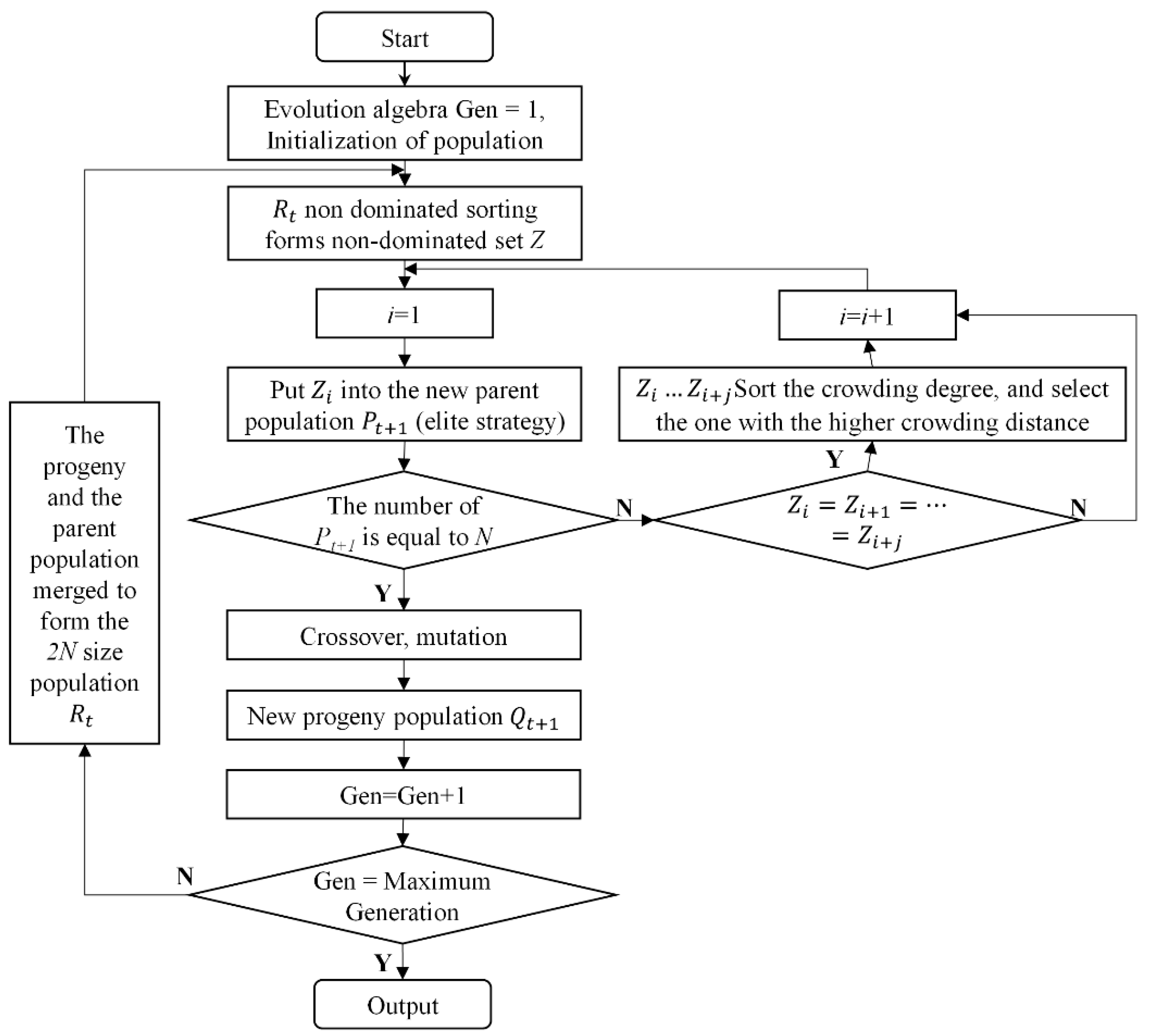
The traditional genetic algorithm (GA) is most suitable for single-objective optimization problems. To solve multi-objective problems, Srinivas and Deb [21] proposed using the non-dominated sorting genetic algorithm (NSGA). This algorithm is based on the dominant relationship between the individuals and shared parameters. The algorithm is widely used to solve multi-objective optimization problems. By aiming at the disadvantages of the NSGA, which include its high computational complexity and strong dependence on the shared parameters, Deb [22] et al. introduced an elite strategy and crowding operator to form the NSGA-II algorithm on the basis of the original algorithm. The algorithm does not need to specify the shared parameters, and it thus has a lower computational complexity and better performance than the NSGA algorithm. The basic operation process of the NSGA-II algorithm is shown in Figure 1.

2.3. Multi-Objective Optimal Regulation Model Coupled with the Hydrodynamic Process

Simulation and optimization are important technical means for water resource system scheduling [23]. The combination of the simulation model and optimization technology can simulate the response process of the entire system under different control schemes. In addition, a combined method provides feedback from the simulation or the evaluation results to the optimization model in order to obtain the optimal operation strategy under known working conditions, and this process is repeated until the system performance reaches the optimal state. This method is one of the most widely used methods in reservoir (group) operation [24], but it is rarely used in cascade gates group water diversion projects.

In this study, a multi-objective optimal regulation model of the cascade gates group that is based on a simulation optimization idea was constructed. In the hydrodynamic model, the change process of the water regime (e.g., water level, discharge, etc.) of the control section under the dynamic control of the cascade gates group was calculated. In the optimization model, when considering the difference and the diversity of the dispatching demand under the different control modes, multiple control objectives need to be set. For optimization, the multi-objective optimization algorithm was used to solve the construction model to reflect the game relationship between the different objectives. The computational framework of the simulation optimization method is illustrated in Figure 2.

2.3.1. Objective Function

The purpose of the normal regulation of the cascade gates group is to maintain the water level of the control section near the target water level on the premise of meeting the water demand of the gate. The normal water level before the gate is usually used [25] to maintain a relatively stable water depth in front of each gate. Therefore, it is necessary to make use of less gate regulation to return the water level to the target water level as soon as possible. Therefore, the optimal operation model was optimized by setting the following target functions:

(1) The average deviation between the operation water level and the target water level is the minimum.

$$min{F}_1=\min \left\{\frac{1}{T·N}{\displaystyle \sum }_{t=1}^T{\displaystyle \sum }_{n=1}^N\left|Z_{tn}-Z_{gn}\right|\right\},t=1,2,\dots ,T,n=1,2,\dots ,N$$

(6)

where $F_1$ is the average deviation between the operation water level and the target water level (m); T is the entire regulation period; N is the number of gates; $Z_{tn}$ is the water level in front of gate n at time t (m); and $Z_{\mathrm{g}n}$ is the target water level of the channel pool n (m).

(2) The number of gate regulations is the lowest in the scheduling period.

$$min{F}_2=\min \left\{c\right\}$$

(7)

where c is the number of gate regulation times in the dispatching period.

2.3.2. Decision Variables and Constraints

In the multi-objective optimal operation model of the cascade gates group, the decision variable is the opening variation of each control gate. The opening amplitude satisfies the following constraints.

$$e_{t,i}^{min}\le e_{t,i}\le e_{t,i}^{max}$$

(8)

where $e_{t,i}^{min}$ is the minimum allowable opening amplitude of a single adjustment at time t for the i^th control gate, m; and $e_{t,i}^{max}$ is the minimum allowable opening amplitude of a single adjustment at time t for the i^th control gate, m.

At the same time, to prevent the lining damage that is caused by the excessive water pressure difference inside and outside the channel slope, the falling speed of the channel water level should not exceed the allowable design value. According to the regulations that are specified by the U.S. Bureau of Reclamation, the water level variation of a concrete-lined channel should meet the following constraints [26].

$$\{\begin{array}{l}\left|Z_{\left(t+1\right),i}-Z_{t,i}\right|\le Z_h=0.15\\ \left|Z_{\left(t+24\right),i}-Z_{t,i}\right|\le Z_d=0.30\end{array}$$

(9)

where $Z_h$ is the change amplitude of the water level per hour (m); $Z_d$ is the change amplitude of the water level per day (m); t is the number of hours, $t=1,2,\dots ,T$; and i is the gate number, where $n=1,2,\dots ,N$.

3. Application

3.1. Study Area

The MRP is a major piece of strategic infrastructure to alleviate the serious shortage of water resources in the Huang Huai Hai Plain and to optimize the allocation of water resources. The total length of the MRP is 1432 km, and it has an average annual water transfer of 9.5 billion m³. The water is diverted from the head gate of the Taocha Channel in the Danjiangkou Reservoir to Tuancheng Lake in Beijing and the Waihuan River in Tianjin. Since the entire water supply line was opened in December 2014, the cumulative water delivery volume of the project has exceeded 25.5 billion m³. This greatly alleviates water shortage in the cities of the water-receiving area, and the water quality of the rivers and lakes along the line has been significantly improved.

The MRP is a typical cascade gates group open-channel water diversion project, and there are 64 gates in total. There is no regulation along the project, which depends on the volume capacity of the channel itself, making the regulation of the project very difficult. Presently, the general dispatching center of the MRP mainly adopts the manual experience dispatching mode, and there are objective problems such as the disunity of the ideas in multi-person alternate regulation. This makes it easy to produce the phenomenon known as secondary regulation, and there are practical engineering problems such as low control accuracy and large labor consumption.

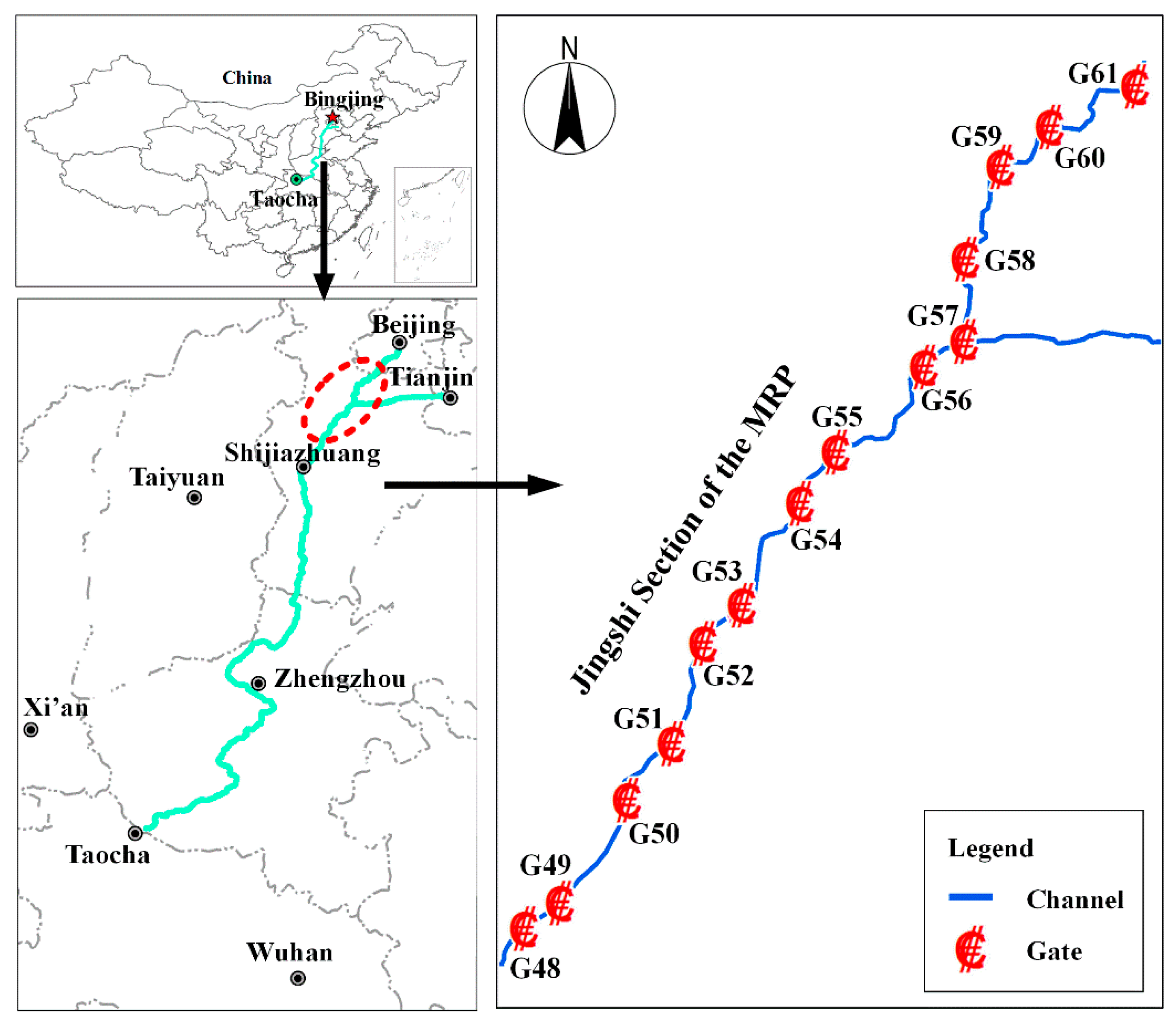
In this study, the Jingshi section of the MRP was used as an example. It applied the optimized control model of the cascade gates group to jointly control the typical working conditions of the cascade gates group that are involved in the area during different operation periods. The total length of the Jingshi section of the MRP was 227 km (Figure 3). From the ancient canal control gate (G48) to the Beijuma River control gate (G61), a total of 13 control gates (excluding G61), 13 diversion gates, and 12 exit gates were involved. The various buildings and basic information on the water delivery channels are presented in

Table 1. Basic information of the control gates in the Jingshi section of the MRP.

Control Gate No.	Stake No.	Gate Bottom Elevation (m)	Single Hole Width (m)	Number of Holes
G48	970 + 379	70.403	6.6	3
G49	980 + 116	67.787	6.0	3
G50	1002 + 169	66.721	6.0	3
G51	1017 + 385	65.344	6.0	3
G52	1036 + 963	64.554	5.5	3
G53	1046 + 196	63.785	5.5	3
G54	1071 + 847	65.151	7.0	3
G55	1085 + 024	61.643	6.0	3
G56	1112 + 074	60.588	7.8	2
G57	1121 + 840	60.783	5.0	3
G58	1136 + 825	57.492	5.0	2
G59	1157 + 652	55.764	5.5	2
G60	1172 + 353	55.596	5.4	2
G61	1197 + 669	55.974	—	2

,

Table 2. Basic information of the diversion gates in the Jingshi section of the MRP.

Diversion Gate No.	Stake No.	Diversion Gate No.	Stake No.
F63	983 + 866	F69	1079 + 569
F64	1007 + 496	F70	1104 + 313
F65	1030 + 769	F71	1117 + 631
F66	1036 + 023	F72	1156 + 414
F67	1061 + 371	F73	1180 + 707
F68	1070 + 370	F74	1195 + 724
F86	1121 + 720

,

Table 3. Basic information of the exit gates in the Jingshi section of the MRP.

Exit Gate No.	Stake No.	Exit Gate No.	Stake No.
T42	977 + 801	T48	1096 + 976
T43	993 + 346	T49	1110 + 179
T44	1015 + 126	T50	1135 + 088
T45	1044 + 822	T51	1157 + 002
T46	1077 + 350	T52	1184 + 713
T47	1084 + 675	T53	1197 + 636

and

Table 4. Basic information of the channels in the Jingshi Section of the MRP.

Channel Pool No.	Entrance	Outlet	Entrance Bottom Elevation (m)	Outlet Bottom Elevation (m)	Bottom Width (m)	Slope Coefficient	Design Roughness
C1	G48	G49	70.403	69.821	10.0–22.2	2.5–3.0	0.014
C2	G49	G50	69.987	69.129	18.0–23.5	2.0–3.0	0.014
C3	G50	G51	68.879	68.360	18.0–21.5	2.5–3.0	0.014
C4	G51	G52	67.574	66.513	18.0–22.0	2.5–3.0	0.014
C5	G52	G53	66.284	65.998	15.0–16.5	3.0	0.014
C6	G53	G54	65.985	65.151	18.7–23.0	2.0–2.5	0.014
C7	G54	G55	65.151	64.264	18.5–23.0	2.0–2.5	0.014
C8	G55	G56	64.140	61.525	15.0–23.0	1.0–2.5	0.014
C9	G56	G57	61.143	60.783	18.5–22.5	0.75–2.5	0.014
C10	G57	G58	60.679	59.877	14.5–20.0	1.0–2.5	0.014
C11	G58	G59	59.767	58.649	7.5–12.5	0.8–2.5	0.014
C12	G59	G60	58.542	57.788	7.5–12.1	0.75–2.5	0.014
C13	G60	G61	57.696	55.974	7.5–13.0	0.75–2.5	0.014

.

3.2. Model Validation

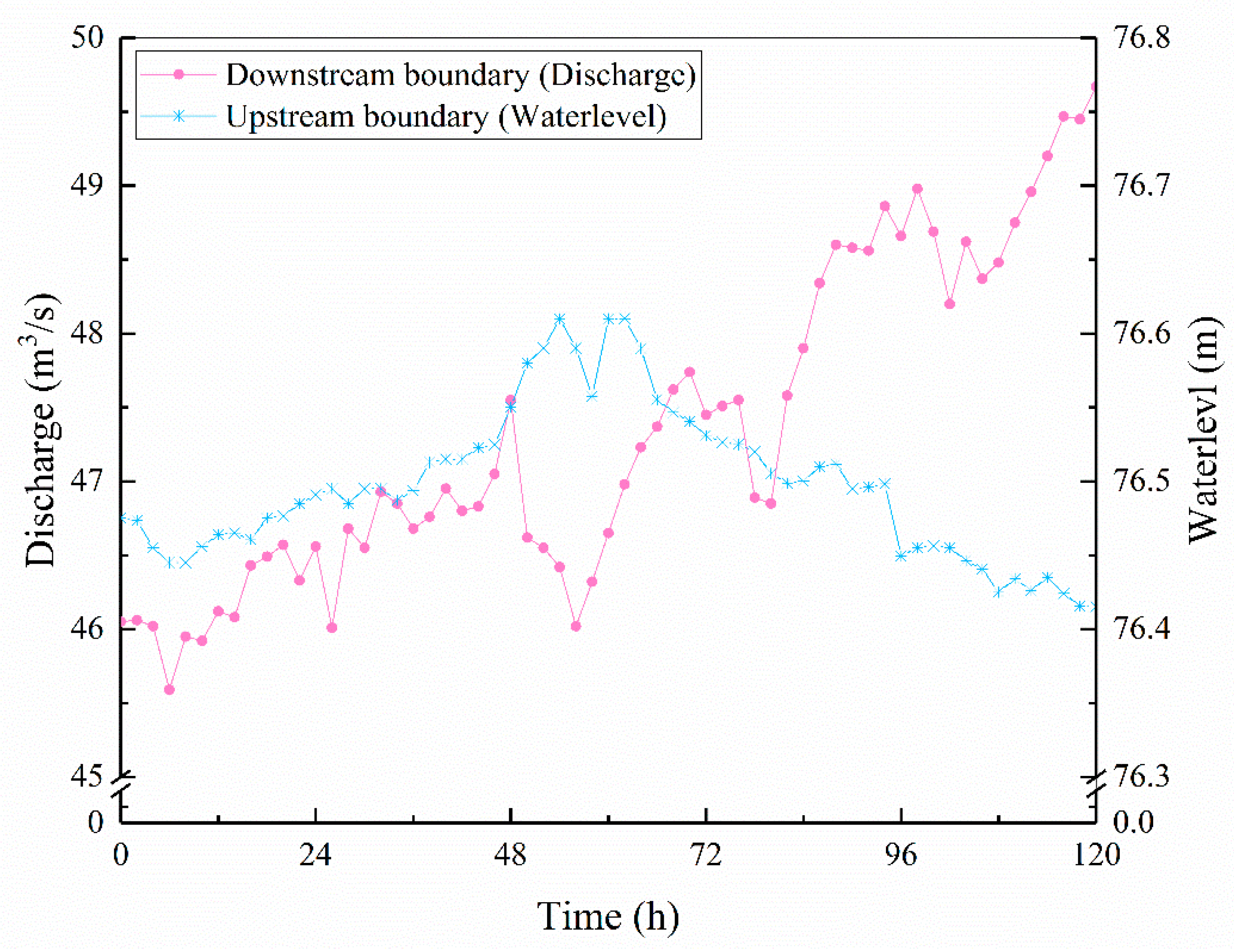
During the operation of the Jingshi section, the downstream boundary water demand increased during the flow adjustment period. This period was selected to build the multi-objective optimization control model of the MRP based on the simulation optimization method. The boundary conditions of the model were set as shown in Figure 4. It can be observed from the figure that the adjustment amount of the downstream flow within 120 h was 4.08 m³/s.

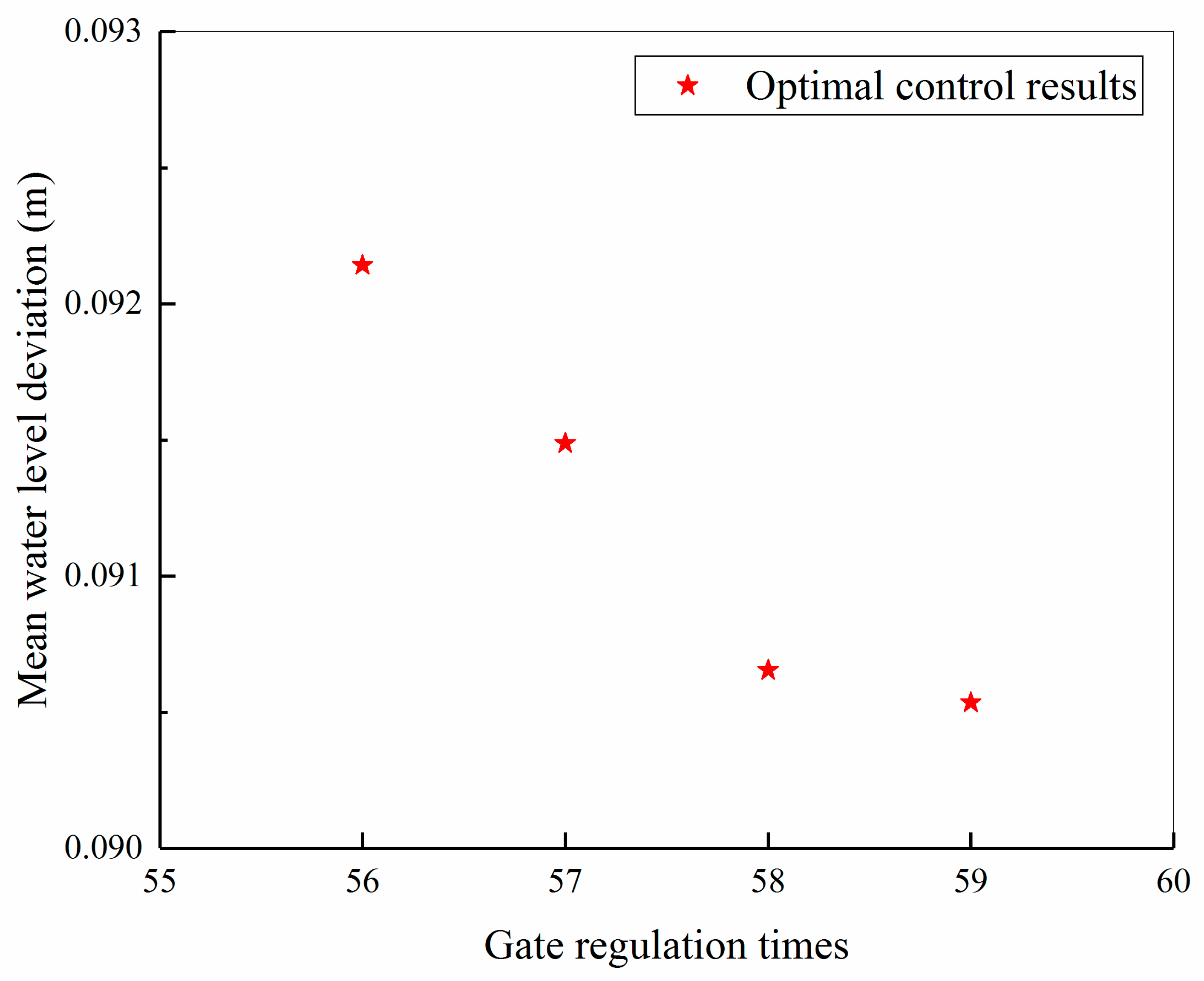
The results of the multi-objective optimization are shown in Figure 5. It can be observed from the figure that there is a game relationship between the number of gate regulations and the average water level deviation after the flow. However, due to the small flow adjustment and small water level deviation, the average water level deviation does not change significantly with the increase in the gate adjustment times in the game relationship.

The operation mode of the stable water level before the control gate is typically used in the MRP. Therefore, a group of solutions with the smallest average water level deviation from the optimization results was selected as the optimal control scheme in this study. The number and average water level deviation of the gate regulation under this scheme are listed in

Table 5. Number and average water level deviations of the gate regulations.

Target	Gate Regulation Times		Mean Water Level Deviation (m)
Contrast	Actual Regulation	Optimal Regulation	Actual Regulation	Optimal Regulation
G48	2	3	0.043	0.042
G49	4	7	0.027	0.059
G50	4	4	0.051	0.035
G51	5	4	0.082	0.060
G52	6	7	0.113	0.019
G53	6	5	0.077	0.019
G54	5	4	0.087	0.038
G55	6	4	0.093	0.042
G56	6	7	0.053	0.086
G57	4	3	0.059	0.085
G58	9	2	0.025	0.095
G59	10	4	0.023	0.098
G60	10	5	0.018	0.099
Total/Average	77	59	0.058	0.060

. It can be observed from the table that the average water level deviation when optimizing the control is not that different from the actual control process and they are all within 0.10 m. However, optimized control can reduce the number of gate control instances by about 23.38%, thus reducing the gate loss and the engineering safety problems that are caused by frequent gate adjustment. Therefore, on the premise of guaranteeing the stability of the water level in front of the control gate, the optimum regulation can compensate for the practical engineering problems of high labor consumption and regulation frequency that are caused by the manual experience regulation, and it can generate an operable gate group regulation scheme.

3.3. Optimum Regulation of the Control Gates Group under Typical Operating Conditions

3.3.1. Typical Working Condition Settings

The flow period is a stage where the flow of the water diversion and water supply of the MRP change significantly. This includes the ice period–non-icing period switching process and the normal operation of the small flow–large flow ecological water replenishment switching process. If the gate group control is implemented after the water demand changes, the upstream and downstream flows will not be matched in time. In addition, the difference in the flow of the entrance and the outlet of the channel pool will cause the volume to change sharply. This will cause the water level to fluctuate significantly and this will affect the safety of the project. Therefore, the feedforward control mode must be adopted during the flow adjustment period. In addition, a reasonable gate group adjustment strategy must be formulated and implemented before water adjustment occurs. This is done to reduce water level fluctuation and restore stability as soon as possible.

According to project scheduling experience, when there is a large flow adjustment at the end of the Jingshi section, it is necessary to control the gate group from one day to three days in advance. To explore the optimal feedforward time under the different flow adjustment ranges, this study set up scenarios in which the feedforward control times were 72, 48, 24, 12, 6, and 4 h, respectively, where the flow adjustment was 10 and 20 m³/s (Table 2), respectively, and the optimal scheduling period was 120 h.

Boundary condition settings are presented in

Table 6. Working condition settings.

Feedforward Time (h)	Working Condition	Flow (m³/s)	Upstream Boundary (Water Level) (m)	Downstream Boundary (Initial Discharge) (m³/s)
72	Condition 1 (C1)	10	76.49	23.26
	Condition 7 (C7)	20
48	Condition 2 (C2)	10
	Condition 8 (C8)	20
24	Condition 3 (C3)	10
	Condition 9 (C9)	20
12	Condition 4 (C4)	10
	Condition 10 (C10)	20
6	Condition 5 (C5)	10
	Condition 11 (C11)	20
4	Condition 6 (C6)	10
	Condition 12 (C12)	20

. The upstream boundary water level is 76.49 m, and it remained unchanged during the regulation process. The initial discharge of the downstream boundary was 23.26 m³/s. The discharge increased by 2 m³/s every 2 h during the flow adjustment period, with a total adjustment of 10 and 20 m³/s.

3.3.2. Initial Condition

The initial state of each control gate under the setting conditions is shown in the Supplementary Materials.

The hydrodynamic simulation of the optimal operation model adopted a calculation time step of 2 min. By combining the requirements of the feedforward control mode for control accuracy, the time interval of each control gate can be adjusted to 12 h, that is, two times a day, and the number of variables in the optimization model was 2 (times) × 5 (days) × 13 = 130.

4. Results and Discussion

4.1. Optimize the Control Results

The optimal operation model of the cascade gates group was used to optimize the aforementioned conditions. A scheme with the minimum water level deviation in the multi-objective is discussed as an example. The results are listed in

Table 7. Multi-objective optimization results.

Working Condition	Average Water Level Deviation (m)	Gate Regulation Times
C1	0.125	67
C2	0.101	71
C3	0.144	73
C4	0.176	66
C5	0.160	72
C6	0.183	73
C7	0.104	83
C8	0.085	86
C9	0.183	92
C10	0.202	86
C11	0.206	82
C12	0.204	90

.

It can be observed from the optimization results that when the downstream discharge of the cascade gates group water diversion project was adjusted, the flows of 10 and 20 m³/s could be adjusted, and the feedforward times were = 72, 48, 24, 12, 6, and 4 h, respectively. A group of optimal control schemes could be obtained by optimizing the control model, and the results are shown in Table 3. It can be observed that when the flow was 10 and 20 m³/s, the feedforward control times were more than 24 h (C1, C2, C7, C8), and the average water level deviation was less than 0.15 m. At this time, the larger the flow adjustment is, the more the gate becomes regulated, but the water level deviation was within the allowable range. When the current feedforward control time was less than 24 h (C3–C6, C9–C12), the average water level deviation was about 0.20 m, and it exceeded the allowable range at this time. To meet the demand of the downstream flow adjustment, more gates are needed to participate in the regulation. Thus, the number of gate regulations was greater than the longer feedforward control time.

4.2. Response Process of the Water Level

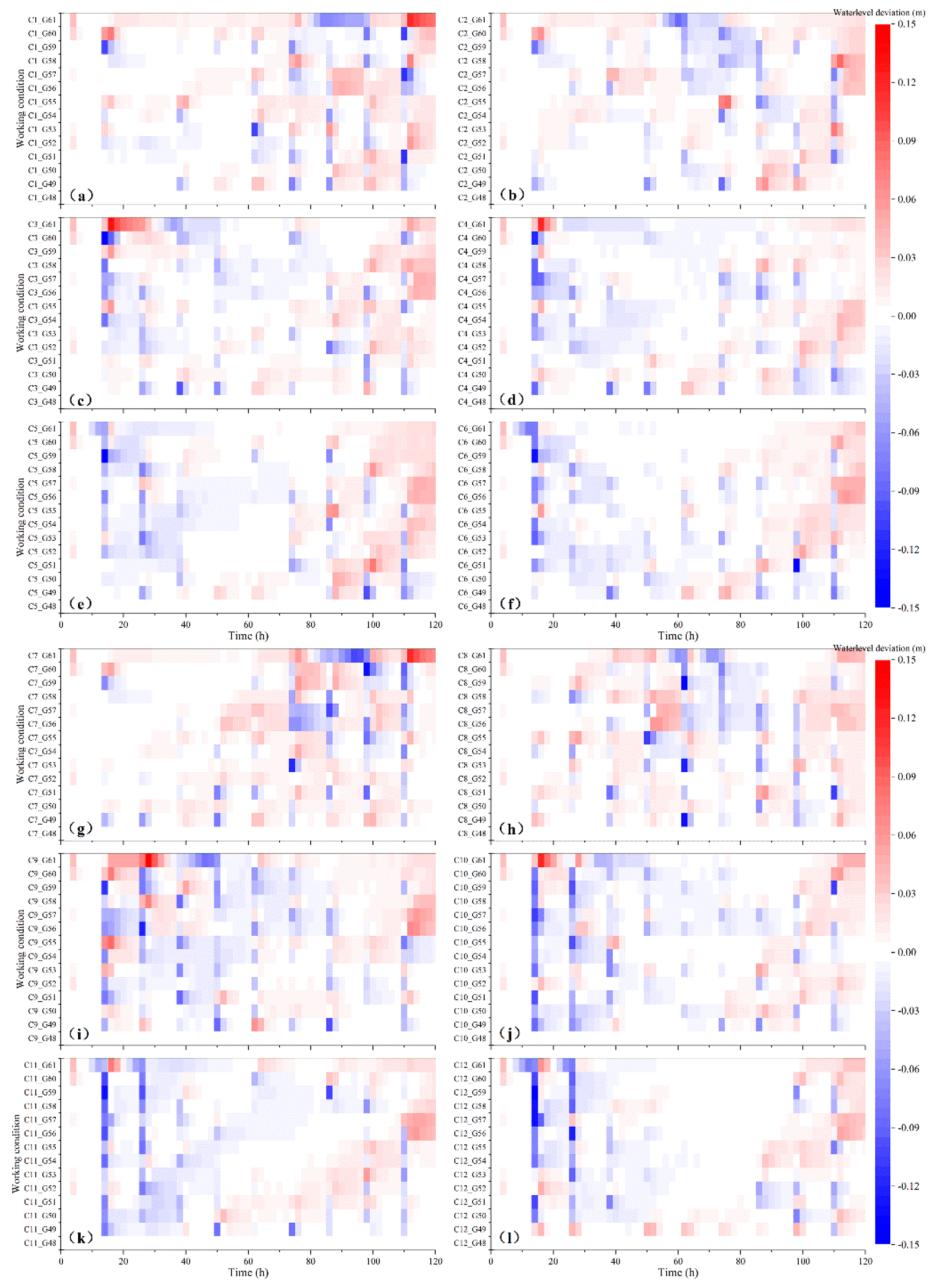
The water level deviation in front of each control gate under the optimization scheme is shown in Figure 6, which reflects the change in the water level of each control section relative to the target water level, revealing the basic mechanism of the cascade gates group system to maintain water level stability during feedforward control. The following can be observed:

(1) When the feedforward control time exceeded 24 h, before the flow adjustment, the water level of each control gate fluctuated slightly. During the discharge adjustment process, the water level before the upstream control gate (upstream of G55) increases slightly, and the water level in front of the downstream control gate (downstream of G55) decreases. When the adjustment is completed, the water level of each control gate is in a stable state near the target water level, and the deviation from the target water level is small.

(2) When the feedforward time is less than 24 h, the upstream water level rises gradually before the flow to store the water from upstream, while the downstream water level tends to be stable. During the flow adjustment period, the storage of the downstream channel pool is preferentially used to supplement the downstream flow adjustment; hence, the downstream water level decreases gradually. After the flow adjustment was completed, the downstream water level gradually began to rise, and it is slightly higher than the target water level.

Figure 6. Water level deviation when the flow adjustment was 10 m³/s and 20 m³/s. (a–l) shows the water level deviation results under working conditions C1–C12 respectively.

Figure 6. Water level deviation when the flow adjustment was 10 m³/s and 20 m³/s. (a–l) shows the water level deviation results under working conditions C1–C12 respectively.

When comparing Figure 6a–f and Figure 6g–l, it can be observed that when the feedforward control time is more than 24 h, the variation law of the water level deviation that is caused by the flow is basically the same, but when the flow adjustment is large (20 m³/s), the deviation is larger. The feedforward control time did not exceed 24 h. The shorter the feedforward control time, the greater the difference between the water levels before and after the flow adjustment. The downstream water level rises before the adjustment, and the downstream water level drops within a short time after the adjustment. The greater the flow adjustment, the greater the drop. After a period of time once the regulation is completed, the upstream water level drops slightly while the downstream water level rises.

4.3. Response Process of the Volume Capacity of the Channel Pool

The volume capacity variation of each channel pool in the optimization scheme is shown in Figure 7. When the feedforward time was more than 24 h, the volume capacity of each channel pool increased slightly after the regulation was completed. When the feed-forward time was less than 24 h, to meet the demand of the downstream flow increase, the volume capacity of the channel pool near the upstream decreased. In addition, the water from the upstream channel pool was used to first supplement the downstream channel pool. After the flow adjustment was completed, the volume capacity of the downstream channel pool increased. When comparing Figure 7a–f and Figure 7g–l, it can be observed that by having a greater downstream water demand, there is a greater volume change for each channel.

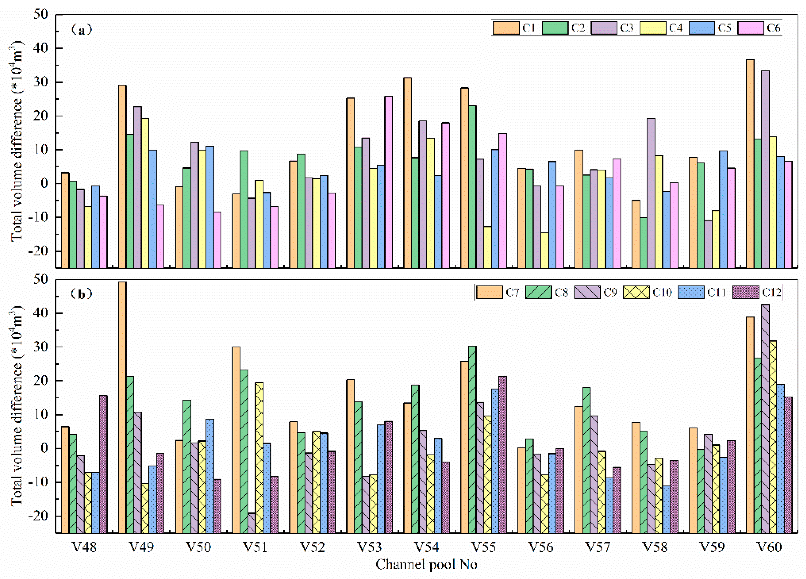
The volume variation of each channel pool with the different feedforward control times is shown in Figure 8. It can be observed from the figure that, when the feedforward control time was approximately 24 h, the volume variation of the channel pool decreased with a reduction in the feedforward control time. When the current feedforward control time was less than 24 h, the volume variation of the channel pool increased, with a decrease in the feedforward control time.

The total volume difference of the system with the different feedforward control times is listed in

Table 8. Total volume difference of the system.

Working Condition	Total Volume Difference of the System (×104 m³)	Working Condition	Total Volume Difference of the System (×104 m³)
C1	173.5460	C7	220.9510
C2	95.7520	C8	183.1010
C3	115.0820	C9	50.3860
C4	33.4700	C10	30.3700
C5	61.2320	C11	24.8800
C6	49.0320	C12	29.4670

. It can be observed from the table that when the feedforward control time exceeds 24 h, there is a greater increase in the total volume in the system with a longer control tim. When the feedforward control time is less than 24 h, the increase in the total volume is small. However, it does not show the law of reduction with the shortening of the feedforward time. It can be observed that, to meet the increase of the downstream water demand when the current feeding time is sufficient (more than 24 h), the system increases the inflow in advance through the upstream boundary, and the increase is large. As a result, the total volume of the system increases greatly. When the current feeding time is short (less than 24 h), the original volume of each channel pool in the system is given priority. Afterwards, the upstream water is used to supplement each channel pool to maintain a stable water level in the system. The increase in the total volume is small.

5. Conclusions

Based on the idea of simulation and optimization, a multi-objective optimal regulation model of a cascade gates group was established. This was achieved by coupling a one-dimensional hydrodynamic model with a multi-objective genetic algorithm (NSGA-II). The model takes the gate opening change as the decision variable, and it can quickly generate the control scheme for the local operation. Taking the Jingshi section of the MRP as an example, by setting different flow adjustment amounts and feedforward control times, the hydrological state and regulation scheme under the different flow adjustment amounts and feedforward control times were analyzed. The results are as follows:

(1) The optimal operation model based on the multi-objective genetic algorithm was better than the conventional control method, and the number of gate operations was reduced by 23.38%.

(2) The average water level deviation was less than 0.15 m when the feedforward control time was more than 24 h, and it was about 0.20 m when the feedforward control time was less than 24 h.

(3) The basic mechanism of the cascade gates group system is to maintain the water level stability in the short-term scheduling. This makes use of the volume capacity or the space that is adjacent to the channel pool in advance.

(4) The limit value of the feedforward control time of the cascade gates group system can reach 4 h. To maintain systems safety and reduce the cost, the optimal feedforward control time should be 24 h.

The multi-objective optimal regulation model of the cascade gates group that was constructed in this study can quickly generate a local operation-oriented regulation scheme for different application scenarios. As a result, this provides good support for the intelligent scheduling of cascade gates group systems.

References

- Wang, Y.; Li, W.; Fang, W. Optimized dispatch of flood control of cascade gate group on river channel in irrigation area. J. Nat. Disasters 2011, 20, 51–56. [Google Scholar]
- Clemmens, A.J.; Kacerek, T.F.; Grawitz, B.E.A. Test Cases for Canal Control Algorithms. J. Irrig. Drain. Eng. 1998, 124, 23–30. [Google Scholar] [CrossRef]
- Cui, W.; Chen, W.; Mu, X.; Bai, Y. Canal controller for the largest water transfer project in China. Irrig. Drain. 2014, 63, 501–511. [Google Scholar] [CrossRef]
- Cui, W.; Chen, W.; Mu, X.; Guo, X. Anticipation time estimation for feedforward control of long canal. J. Hydraul. Eng. 2009, 40, 1345–1350. [Google Scholar]
- Fan, Y.; Gao, Z.; Chen, H.; Wang, S.; Chang, H. Analysis of canal feedforward control time based on constant water volume. J. Drain. Irrig. Mach. Eng. 2018, 36, 1131–1136. [Google Scholar] [CrossRef]
- Wu, H.; Lei, X.; Qin, T.; Xu, H.; Wang, H. Operation control of storage compensation of canal system in the Middle Route of South-to-North Water Diversion Project. South-North Water Transf. Water Sci. Technol. 2015, 13, 788–792. [Google Scholar]
- Yao, X.; Wang, C.; Li, C. Operation mode of serial canal system based on water volume control method. J. Hydraul. Eng. 2008, 39, 733–738. [Google Scholar] [CrossRef]
- Malaterre, P.; Rogers, D.C.; Schuurmans, J. Classification of Canal Control Algorithms. J. Irrig. Drain. Eng. 1998, 124, 3–10. [Google Scholar] [CrossRef] [Green Version]
- Wahlin, B.; Zimbelman, D. Canal Automation for Irrigation Systems: American Society of Civil Engineers Manual of Practice Number 131. Irrig. Drain. 2018, 67, 22–28. [Google Scholar] [CrossRef]
- Robert, S.G.; Eduardo, B.; Robert, J.S. Automated scheduling of open-channel deliveries: Potential and limiations. In SCADA and Related Technologies for Irrigation District Modernization, 2nd ed.; USCID: Phoenix, AZ, USA, 2007; pp. 23–32. [Google Scholar]
- Zhong, K.; Guan, G.; Liao, W.; Xiao, C.; Su, H. Algorithm with variable downstream target depth based on balance of water volume in canal pond. J. Drain. Irrig. Mach. Eng. 2018, 36, 857–862. [Google Scholar]
- Schuurmans, J.; Clemmens, A.J.; Dijkstra, S.; Hof, A.; Brouwer, R. Modeling of Irrigation and Drainage Canals for Controller Design. J. Irrig. Drain. Eng. 1999, 125, 338–344. [Google Scholar] [CrossRef] [Green Version]
- Liu, F.; Feyen, J.; Malaterre, P.; Baume, J. Development and Evaluation of Canal Automation Algorithm CLIS. J. Irrig. Drain. Eng. 1998, 124, 40. [Google Scholar] [CrossRef]
- Bautista, E.; Clemmens, A. Volume Compensation Method for Routing Irrigation Canal Demand Changes. J. Irrig. Drain. Eng. 2005, 131, 494–503. [Google Scholar] [CrossRef] [Green Version]
- Parrish, J. A Methodology for Automated Control of Sloping Canals; University of Iowa: Lowa City, IA, USA, 1997. [Google Scholar]
- Yao, X.; Wang, C.; Ding, Z.; Li, J. Study on Canal System Operation Based on Discharge Active Compensation. Adv. Eng. Sci. 2008, 40, 38–44. [Google Scholar]
- Malaterre, P.O. PILOTE: Linear Quadratic Optimal Controller for Irrigation Canals. J. Irrig. Drain. Eng. 1998, 124, 187–194. [Google Scholar] [CrossRef]
- Lin, B.; Su, X. Optimal dispatching of flood control system for sluice groups in plain dike areas. J. Zhejiang Univ. (Eng. Sci.) 1996, 30, 652–663. [Google Scholar]
- Liu, Q. Hydraulic Calculation and Optimal Operation of Multi-Sluice Flood Control System in Plain River Network Reion. Master’s Thesis, Hohai University, Nanjing, China, 2006. [Google Scholar]
- Zhu, J.; Zhang, Z.; Lei, X.; Jing, X.; Wang, H.; Yan, P. Ecological scheduling of the middle route of south-to-north water diversion project based on a reinforcement learning model. J. Hydrol. 2021, 596, 126107. [Google Scholar] [CrossRef]
- Srinivas, N.; Deb, K. Muiltiobj ective Optimization Using Nondominated Sorting in Genetic Algorithms. Evol. Comput. 1994, 2, 221–248. [Google Scholar] [CrossRef]
- Deb, K.; Pratap, A.; Agarwal, S.; Meyarivan, T. A fast and elitist multiobjective genetic algorithm: NSGA-II. IEEE Trans. Evol. Comput. 2002, 6, 182–197. [Google Scholar] [CrossRef] [Green Version]
- Guo, X.; Qin, T.; Lei, X.; Jiang, Y.; Wang, H. Advances in derivation method for multi-reservoir joint operation policy. J. Hydroelectr. Eng. 2016, 35, 19–27. [Google Scholar]
- Wang, H.; Wang, X.; Lei, X.; Liao, W.; Wang, C.; Wang, J. The development and prospect of key techniques in the cascade reservoir operation. J. Hydraul. Eng. 2019, 50, 25–37. [Google Scholar]
- Cui, W.; Chen, W.; Mu, X. Dynamic regulation algorithm of volumes for long distance water division canal. J. China Inst. Water Resour. Hydropower Res. 2015, 13, 421–427. [Google Scholar] [CrossRef]
- Buyalski, C.P.; Ehler, D.G.; Falvey, H.T.; Rogers, D.C.; Serfozo, E.A. Canal Systems Automation Manual: Volume 1; US Bureau of Reclamation: Denver, CO, USA, 1991.
Figure 1.
Basic operation process of the NSGA-II algorithm.
Figure 2.
Computational framework of the simulation optimization method.
Figure 3.
Distribution of the control gates in the Jingshi section.
Figure 4.
Boundary conditions during the operation.
Figure 5.
Results of the multi-objective optimization.
Figure 7.
Storage capacity when the flow adjustments are 10 m³/s and 20 m³/s. (a–l) shows the volume capacity variation results under working conditions C1–C12 respectively.
Figure 8.
Total volume difference.