Upper Limit and Power Generation Loss of Water Supplement from Cascade Hydropower Stations to Downstream under Lancang-Mekong Cooperation

Abstract

In cross-border water supplement cooperation, the supplement water discharged from upstream hydropower stations is the key to improving downstream benefits, but will lead to upstream power generation loss, so the upstream hydropower stations have to be aware of how much water they can offer and how much power they will lose to make the water supplement cooperation more reasonable. Therefore, this study puts forward a model to calculate the upper limit flow of water supplement of cascade hydropower stations under firm power constraints and water level constraints and proposes a new optimization method called the “collaborative-independent” joint optimization method to calculate the power generation loss under water supplement constraints. The results show that the upper limit flow will increase with the increase of annual inflow, and the uncertainty of the distribution of inflow in the year will also affect the upper limit flow: the larger the proportion of non-flood season inflow, the higher the upper limit flow. In normal and wet years, delaying water supplement time can significantly increase the upper limit flow by about 5% per month. Additionally, the “collaborative-independent” joint optimization method newly proposed in this paper can significantly improve the local optimization problem compared to the traditional optimization method. The power generation loss increases with the increase of water supplement flow, and delaying water supplement time can significantly reduce the power generation loss. The results of this paper can provide essential data support for future water resources cooperation negotiations in the Lancang-Mekong river basin to promote efficient and orderly water resources cooperation in the basin.

1. Introduction

In recent decades, with the continuous development and utilization of water resources globally, especially in some cross-border river basins, water resource disputes among riparian countries are emerging and becoming increasingly severe [1,2], because the riparian countries may place different demands on a cross-border river [3]. This situation can both create conflicts and provide opportunities for cooperation [4,5]. Many studies have explored various measures to alleviate the water conflicts among these countries [6,7,8,9], and cross-border water resources cooperation is considered as one of the best ways to solve the problem [10,11,12,13]. At present, the global optimization method has been applied to cross-border water resources cooperation in much research, where the water resources utilization strategies of all countries are obtained by optimization to obtain the maximum extra benefit increment of the whole basin, and then allocate the benefits among countries [14,15]. This kind of research evaluates the benefit increment of the basin brought by the cooperation from a macro perspective. However, because the interests of upstream and downstream countries are different, and some interests even have nothing to do with the water resources (such as trade demands, political demands, etc.) [16], it is difficult to quantify the interests of all countries accurately. Therefore, the evaluation results are challenging to be recognized by all the riparian countries, leading to few applications of this method.

The cooperation mode of temporary (emergency) negotiation is common among instances of practical cross-border cooperation [13,17]. Taking the Mekong River Basin as an example, in the dry season of 2016, affected by the El Nino phenomenon, the rainfall in the Lancang-Mekong River Basin decreased significantly. As a result, the drought seriously affected China in the upper reaches and Southeast Asian countries in the lower reaches. Vietnam has requested the Chinese government to release more water through the cascade hydropower stations on the Lancang River to relieve the shortage of agricultural irrigation water. In the face of the impact of the normal power generation plan, the Chinese government still responded positively. From 15 March to 10 April 2016, Yunnan Jinghong Hydropower Station (the most downstream hydropower station on the Lancang River) increased the daily average discharge over 2000 m³/s to implement emergency water supplement for the downstream [18]. This water supplement has dramatically alleviated the drought in countries along the Mekong River, especially Vietnam. As a successful cross-border water resources cooperation practice in the Lancang-Mekong basin, the China-Vietnam water supplement incident in 2016 is a significant reference event. Due to the geographical location and water resources, the interests of upstream China and downstream Southeast Asian countries are relatively independent; as such, this modular cooperation of “application-negotiation-water supplement” is also a direct, efficient mode of cooperation and worthy of further study.

Increasing discharge of hydropower station in non-flood season will lead to a premature reduction of water head, which will undoubtedly harm power generation [19]. However, obviously, the water supplement cooperation is meaningful only when the downstream profit increment after water supplement is greater than the upstream loss. Therefore, to make the cooperation reasonable and sustainable, the upstream cascade hydropower stations must be aware of how much water they can supply and how much power they will lose when they offer different amounts of water to the downstream under the different hydrologic condition. In other words, the upper limit flow (ULF) and power generation loss (PGL) are critical information for the basin cooperation negotiations which determine whether to cooperate or not.

The calculation of the PGL of hydropower station here can be regarded as an operation optimizing problem of hydropower station under changing water supplement constraints (changing flow and time period). Tao et al. [20] calculated the power generation loss of the Longyangxia Hydropower Station by using the method of operation optimization; however, this was only limited to a single reservoir and did not consider the ULF. Because the water storage of cascade hydropower stations is scattered in all levels of reservoirs, the compensation between the upper and lower reservoirs is involved in water supplement. The calculation of the ULF and PGL is much more complex than that of a single reservoir, and there are few pieces of research considering cascade hydropower stations. The operation optimizing of cascade hydropower stations has the strong characteristics of high dimension, non-convexity, and non-linearity. With water supplement constraints, the accurate solution for maximum power generation is more difficult to obtain because the feasible region for decision variables are more irregular under abrupt and complex constraints (water supplement) which makes optimization more difficult. Dynamic programming (DP) [21] and discrete differential dynamic programming (DDDP) [22] can solve the optimal operation problem of cascade hydropower stations with comparatively low accuracy to a certain extent. However, these algorithms based on the principle of dynamic programming will face significant “dimension disaster” and be time-consuming when there are many hydropower stations or high accuracy requirements. Although the algorithms such as POA [23,24] and DPSA [25] can save much time in single optimization by dimension reduction and produce a relatively accurate solution [26], the searching ability of the algorithms is still not enough facing abrupt and complex constraints. Thus, it can be seen that the efficient and accurate operation optimization of cascade hydropower stations under complex constraints is still a thorny problem. Therefore, a method that can give consideration to accuracy and speed and obtain a water compensation strategy between the cascade reservoirs during the water supplement period is urgently needed to carry out the optimal operation of cascade water supplementation.

To sum up, taking China’s cascade hydropower stations on Lancang River as the research object, this paper puts forward the calculation method framework of ULF and PGL of cascade hydropower stations in non-flood season. A “collaborative-independent” joint optimization method is proposed as a new optimization method to obtain a more accurate quantitative relationship between power generation loss and water supplement flow. The results can be used as the basis for water resources negotiation of upstream and downstream modules in the future and guide the water supplement operation to promote the cooperation between upstream and downstream modules to be more reasonable and orderly.

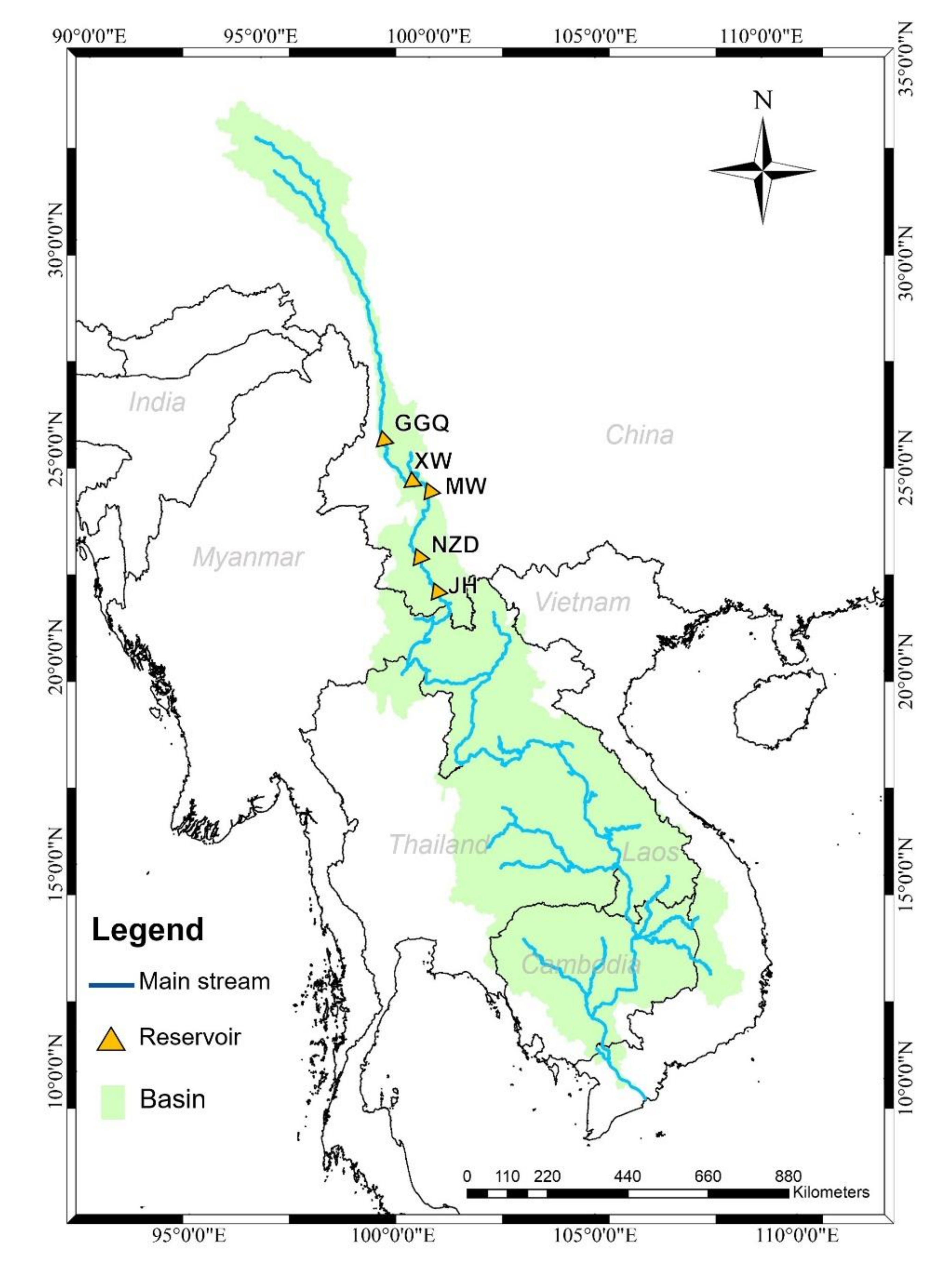
2. Study Area and Data

With a total length of 4880 km, the Mekong River originates from China’s Qinghai Tibet Plateau, flows through China, Myanmar, Laos, Thailand, Cambodia, and Vietnam (as shown in Figure 1), and finally flows into the South China Sea. The upper Mekong River Basin (UMRB), also known as the Lancang River Basin, is located in China, accounting for 13.5% of the average runoff of the Mekong River. The lower Mekong River basin (LMRB) includes the five other countries, contributing 86.5% of the average runoff of the Mekong River [27]. The basin has clear wet and dry seasons and highly seasonal rainfall dominated by the southwest monsoon [28,29]. The Lancang-Mekong River provides a large amount of water for power generation, irrigation, wetland protection and shipping for riparian countries. Due to the intensive water flow and a large span of elevation (1780 m) in Yunnan Province, the section of river in Yunnan Province has very large hydraulic resources, and the technologically exploitable hydropower potential in this section is up to 27,490 megawatts [30], making it one of the thirteen key “hydropower bases” in China [31]. Currently, five major hydropower stations have been built along the mainstream of the Lancang River. The cascade reservoirs from upstream to downstream are Gongguoqiao (GGQ), Xiaowan (XW), Manwan (MW), Nuozhadu (NZD), and Jinghong (JH). The cascade reservoir system has a total installed capacity of 14,370 megawatts (MW) [32]. The two largest reservoirs, XW and NZD, play leading roles in the hydropower operations of the Lancang River, contributing to 36% and 58%, respectively, of the total storage capacity of the five reservoirs. However, the five countries in the LMRB are all agricultural-oriented countries mainly based on rice cultivation. The agricultural water withdrawal of Myanmar, Laos, Thailand, and Cambodia accounts for more than 90% of the total water withdrawal of each country, and that figure in Vietnam also reaches 68% [14]. Therefore, agricultural irrigation is the most crucial water resource benefit of the downstream module.

Through the observation of the characteristics of the Mekong River basin, it is not difficult to find that: (1) the utilization of water resources in China and that five countries in the LMRB are pretty different. China, located in the upper reaches, mainly produces hydropower, while the five countries in LMRB mainly use water for agricultural irrigation. (2) The cascade hydropower stations in China are the water conservancy facilities with the largest storage capacity in the basin. The discharge process of cascade hydropower stations in the non-flood season is the primary human control factor that can determine the water resources benefits (agricultural irrigation benefits) of the five countries in the LMRB. (3) China and the five countries in LMRB have strict upstream and downstream relations. This natural geographical relationship determines that it is difficult for the downstream countries to make the upstream countries actively adjust their strategies by changing their own water resources utilization strategies. Therefore, dialogue and consultation with upstream countries to solve problems have become more practical solutions for downstream countries. This is also the fundamental reason for successfully applying the modular cooperation mode of the “Application-Negotiation-Water supplement” in the basin.

Due to the monsoon climate, the basin has abundant rainfall in the flood season, such that the agricultural water demand can be easily met, and there is no need for upstream water supplement. The period with the greatest risk of drought in the LMBR is from January to May [27], so the default water supplement period in this paper is from January to May.

3. Methodology

Considering the water supplement scenario in Vietnam in 2016, the water supplement lasted for nearly a month. In order to facilitate the study, this paper also simplified the corresponding method, taking the length of the water supplement period and the operation time step as the same, both of which are one month. The storage capacities of GGQ, MW, and JH are much smaller than that of XW and NZD, and they can almost be regarded as runoff power stations when the time scale of the operation model is monthly. Therefore, it can be considered that the water supplement is mainly borne by the impoundment of XW and NZD reservoirs indirectly, and the Lancang River cascade reservoirs can be simplified as a XW-NZD cascade hydropower station, and NZD directly supplements the downstream.

In order to calculate the PGL of the water supplement, this paper optimizes the maximum power generation under different supplement water flow constraints, then the PGL when the supplement water period is t and the supplement water flow is $q_c$ equals to the maximum cascade power generation without water supplement constraint minus that with water supplement constraint $q_c$ in time period t, which can be expressed by:

$$D_j\left(q_c\right)=\max W_0-\max W\left(t,q_c\right)$$

(1)

where $D_j\left(q_c\right)$ is the PGL when the supplement water period is t and the supplement water flow is $q_c$; $W_0$ is the maximum cascade power generation without water supplement constraint; $W\left(t,q_c\right)$ is the maximum cascade power generation with water supplement constraint $q_c$ in time period t.

It can be seen that the essence of calculating PGL is to calculate the maximum power generation of the cascade hydropower stations under different water supplement constraints, that is, the quantitative relationship between water supplement flow and maximum power generation (hereinafter referred to as “flow-energy” relationship). Therefore, first of all, it is necessary to clarify the range of the water supplement flow, that is, the maximum discharge flow of NZD during the water supplement period or ULF.

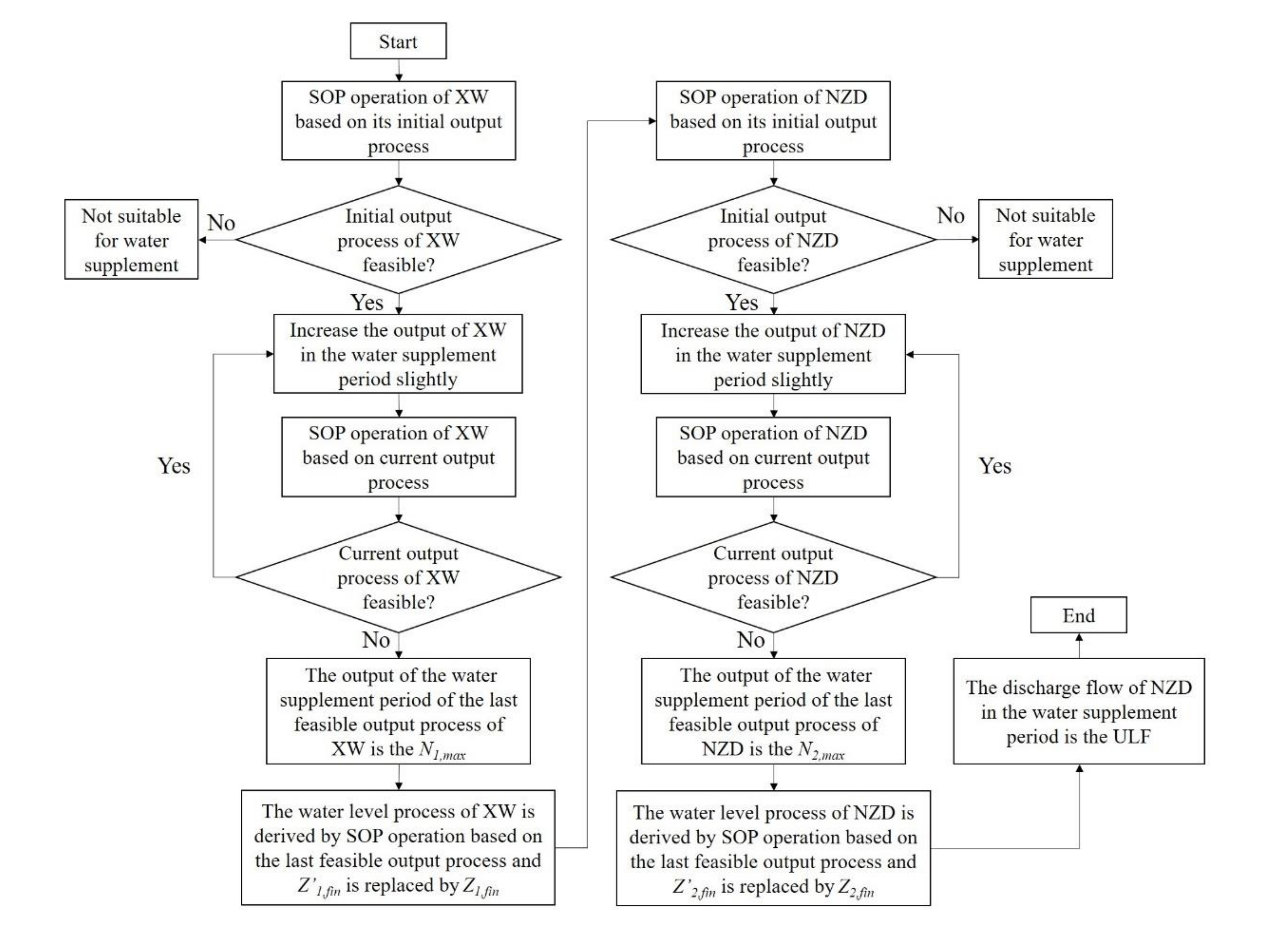
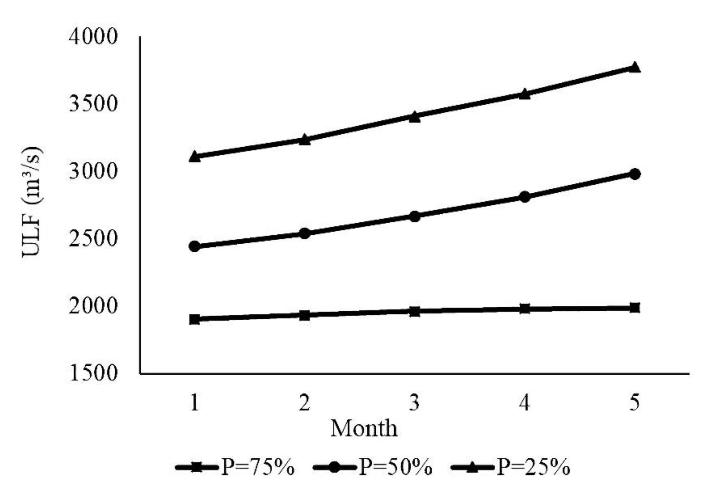
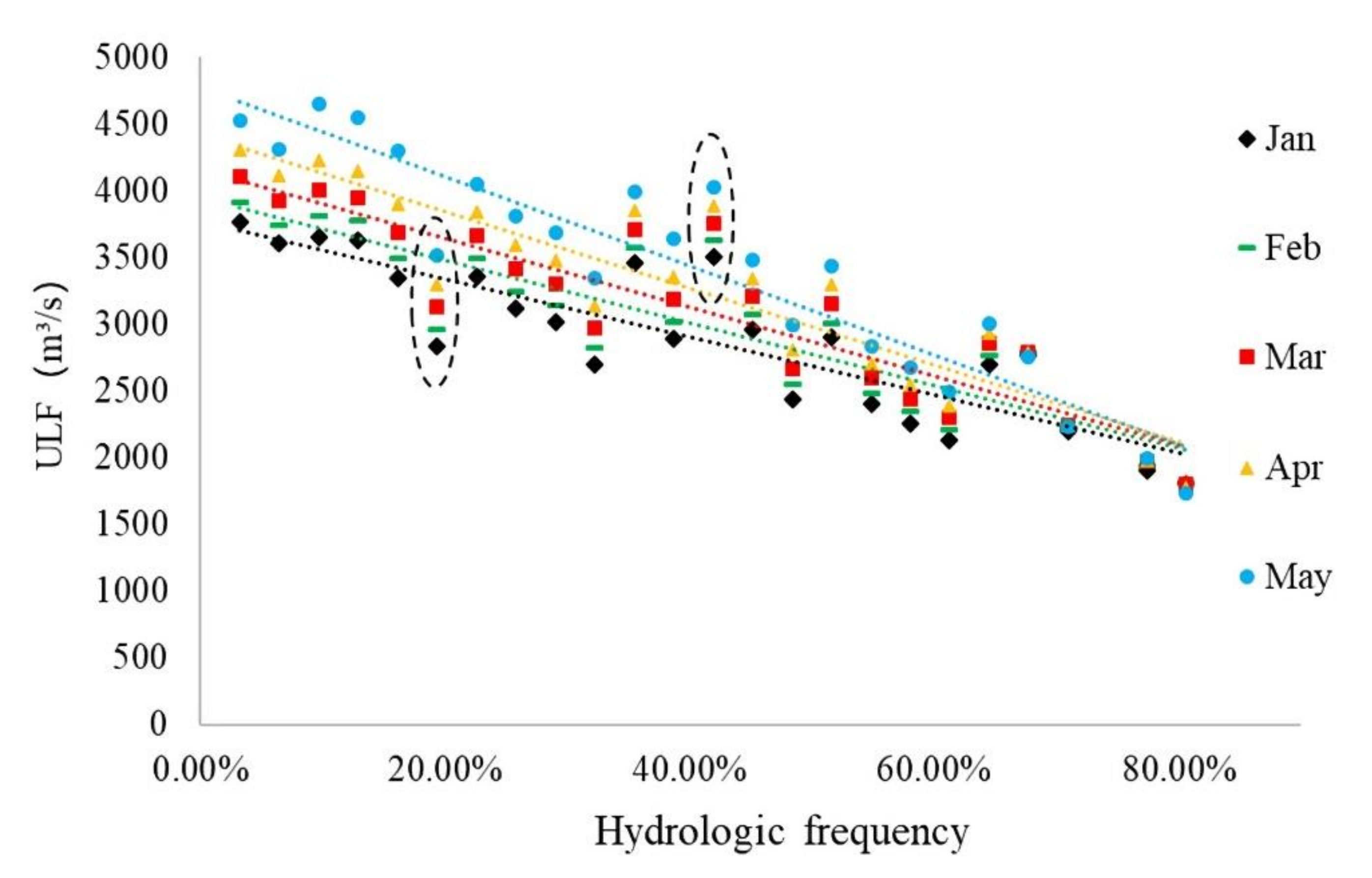
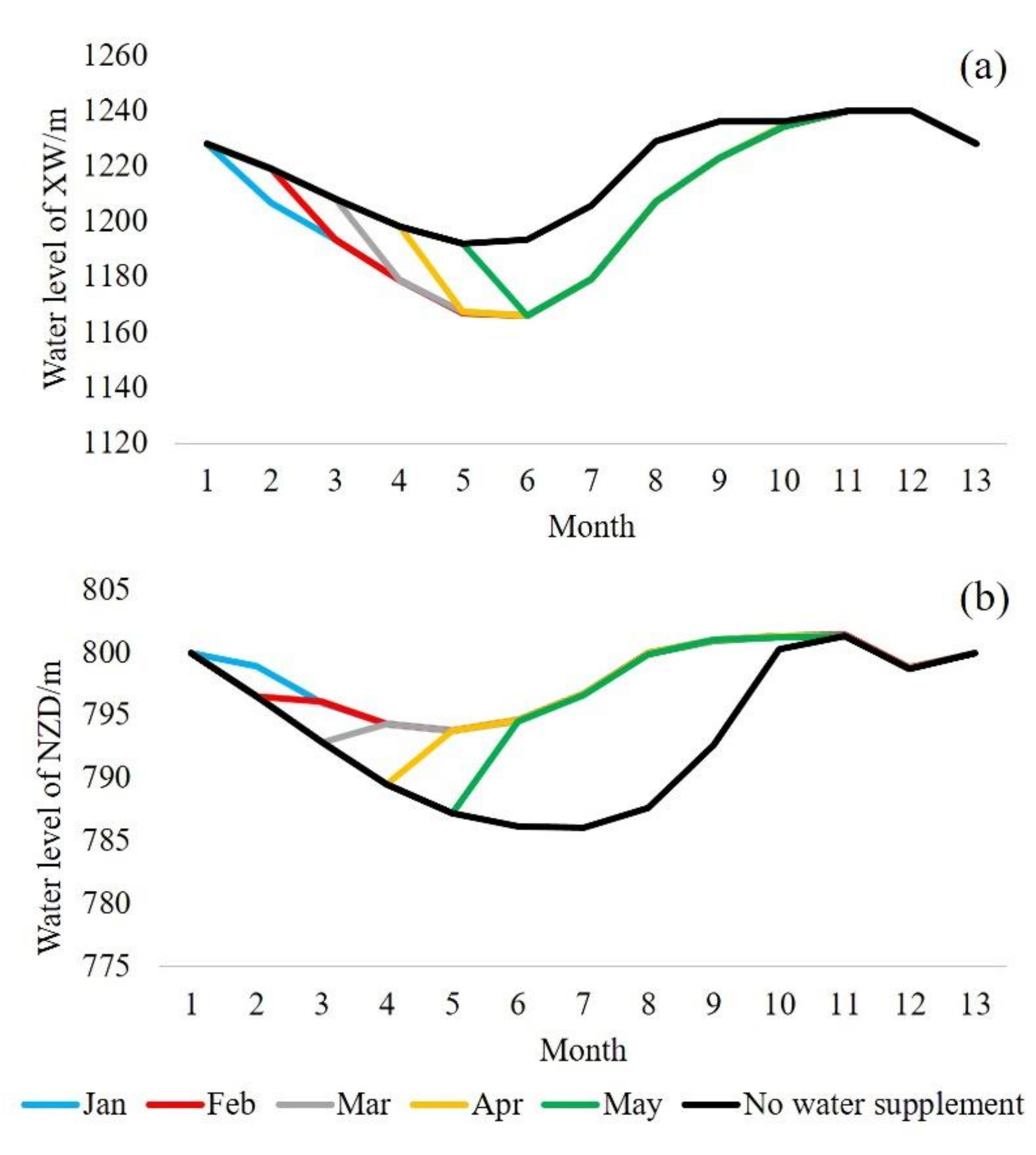
3.1. Calculation of ULF

Before describing the specific method of calculation of ULF, for ease of reading and understanding, the table of Nomenclature (

Table 1. Table of nomenclature.

Term	Explanation
Firm power	Firm power refers to the value that the output of hydropower station, under normal operation, shall not be lower than. If the output in a certain period is lower than the firm power, it indicates that the power generation task is damaged.
Initial output process	Initial output process is the output process in which the ouput in each time period equals to the firm power of the corresponding hydropower station.
Standard operating policy (SOP)	SOP means releasing water just to the meet the output of the hydropower stations in every time period.
Initial water level and final water level constraints	Initial water level means the water level at the beginning of the operation period in each reservoir; and final water level means the water level at the end of the operation period in each reservoir.
Feasible output process	If the SOP operations of the hydropower stations can be completed under the premise of meeting all constraints, and the water level at the end of the operation period is higher than or equal to the final water level constraint, then the output process is feasible, otherwise it is not feasible.

) shows the meanings of four terms that appear later in this section.

Taking one natural year as the operation period, under the premise that both hydropower stations do not break all kinds of constraints (dead water level constraint, final water level constraint, firm power constraint, etc.) in the whole year, the maximum discharge flow of NZD that can be achieved through the cooperation of the hydropower stations during the water supplement period is the ULF, and the state is called the limit state of water supplement. The respective output of two hydropower stations under the limit state is called the limit output.

Then the calculation steps of the limit state of any water supplement period are as follows:

(1)

Set $Z_{1,ini}$ and $Z_{1,fin}$ as the initial and final water level constraints of XW, respectively. Set $Z_{2,ini}$ and $Z_{2,fin}$ as the initial and final water level constrains of NZD, respectively.

(2)

The operation process of XW within the year is carried out by using SOP according to the initial output process of XW. If the initial output process is feasible, enter step (3); otherwise, it indicates that the inflow condition of the year is not suitable for water supplement, which means, even there is no water supplement requirements from the downstream countries, that part of the periods still lacks water, and water supplement may cause greater burden on the upstream power generation task.

(3)

Based on the initial output process of XW, increase the output in the water supplement period gradually (the output of other periods remains unchanged), until continuous increase will cause the output process to be not feasible. Save the water level process derived by SOP and the output of XW in the water supplement period at the time. Record the output of XW as $N_{1,max}$, and the final water level derived by SOP operation now is $Z_{1,fin}^{\prime }$. Due to the fact that $Z_{1,fin}^{\prime }$ must be higher than or equal to $Z_{1,fin}$, replace $Z_{1,fin}^{\prime }$ with $Z_{1,fin}$, and the water level process after the replacement is the final water level process of XW under the limit state of water supplement;

(4)

Keep the final water level process of XW under the limit state of water supplement obtained in step (3) unchanged, and then the operation process of NZD within the year is carried out by using SOP according to the initial output process of NZD. If the initial output process is feasible, enter step (5); otherwise, it indicates that the inflow condition of the year is not suitable for water supplement. Water supplement may cause greater burden on the upstream power generation task.

(5)

Based on the initial output process of NZD, increase the output in the water supplement period gradually (the output of other periods remains unchanged), until continuous increase will cause the output process to be not feasible. Save the water level process derived by SOP and the output of NZD in the water supplement period at the time. Record the output of NZD as $N_{2,max}$, and the final water level derived by SOP operation now is $Z_{2,fin}^{\prime }$. Due to the fact that $Z_{2,fin}^{\prime }$ must be higher than or equal to $Z_{2,fin}$, replace $Z_{2,fin}^{\prime }$ with $Z_{2,fin}$, and the water level process after the replacement is the final water level process of NZD under the limit state of water supplement;

$N_{1,max}$ and $N_{2,max}$ are the maximum output of XW and NZD during the water supplement period, respectively, and the discharge of NZD during the water supplement period is the ULF. In order to facilitate understanding, this paper shows this process in the form of a flow chart, as shown in Figure 2.

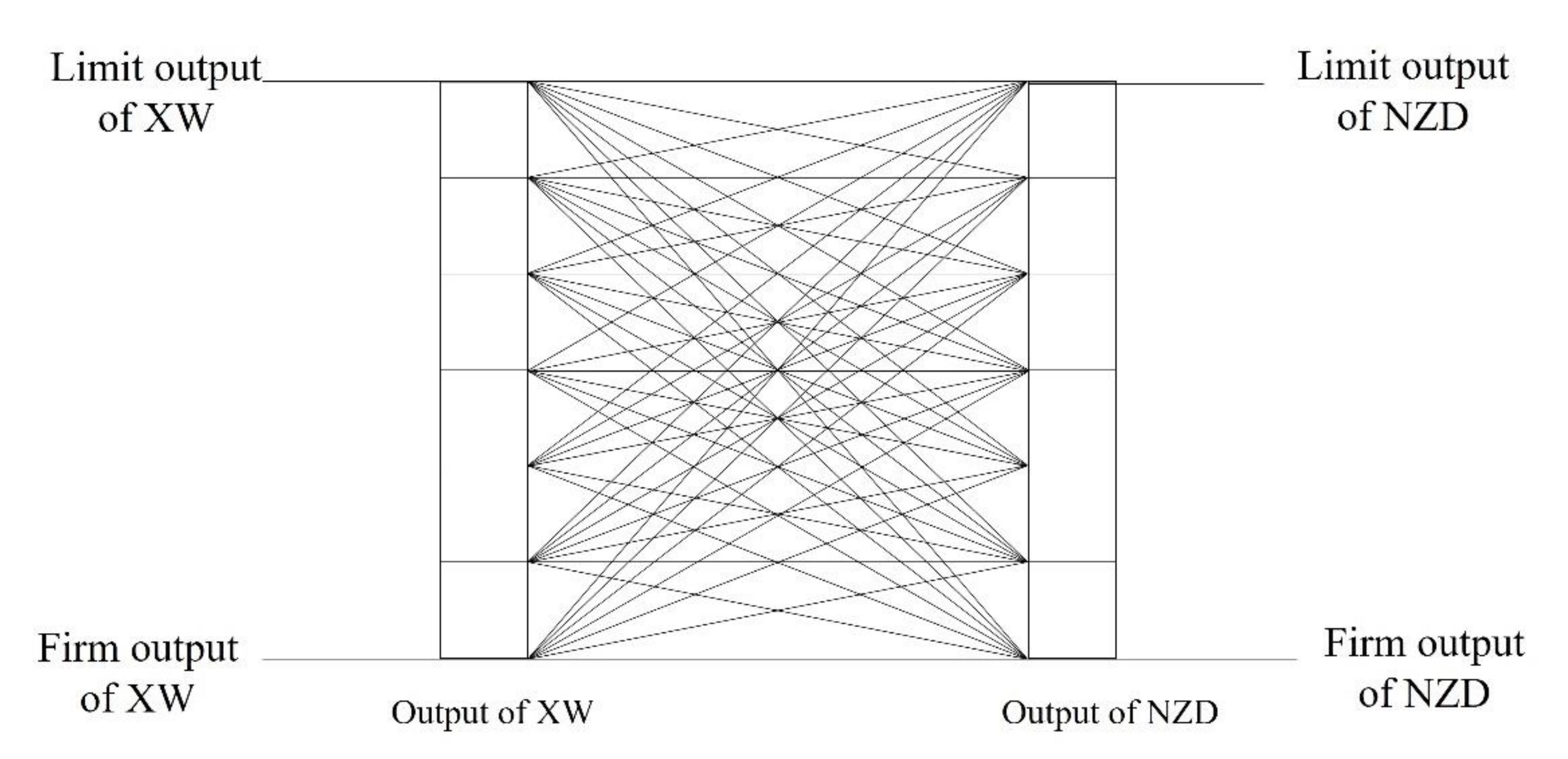
3.2. Optimization of Maximum Power Generation under Water Supplement Constraints

As mentioned at the beginning of section, after the ULF is obtained, the corresponding maximum power generation under different water supplement constraints needs to be optimized, and then the power generation loss can be calculated by Equation (1). As mentioned in the introduction, there are many difficulties in solving the optimal operation of cascade hydropower stations, especially after the addition of the water supplement constraint, because the water supplement constraint is imposed on individual periods, which only affects individual decision variables or the relationship between them. The feasible region of decision variables becomes more irregular, and the difficulty of searching and optimizing increases, so in the process of optimization, the possibility of falling into local optimum also increases sharply. Because this study needs to optimize the cascade power generation in different periods and under different water supplement constraints for many times, the final “flow-energy” relationship is also a result of high precision requirements, so the traditional dynamic programming method is not used because of its serious time-consuming and low precision. In order to calculate the maximum power generation under different water supplement constraints as accurately as possible and obtain a more precise relationship between water supplement flow and power generation, this paper uses the POA algorithm commonly used in the optimal operation of cascade hydropower stations to optimize the power generation under different water supplement constraints by two methods: cascade collaborative optimization and discrete independent optimization. Then, the optimal results of the two methods are taken and complemented to each other in order to alleviate the problem of local optimization.

(1)

Objective function

In this paper, the “water head-water consumption rate” curve is used to calculate the generation capacity of each hydropower station [33]:

$${\eta }_{j,t}=f_j\left(h_{j,t}\right)$$

(2)

$$P_{j,t}=\frac{Q{G}_{j,t}}{{\eta }_{j,t}}\times 3600/1000$$

(3)

$$\max W={\displaystyle \sum }_{t=1}^T{\displaystyle \sum }_{j=1}^k{P}_{j,t}·\Delta t$$

(4)

where j is the serial number of the reservoirs, XW is 1, and NZD is 2; ${\eta }_{j,t}$ (m³/kwh) is the average water consumption rate of reservoir j in time period t, and it depends on h_j,t, the average hydraulic head of time period t; f_j is the relationship between the water consumption rate and average hydraulic head of reservoir j; P_j,t (10⁴ kw) is the output of reservoir j in time period t (3600/10,000 is to transform the unit from kWh/s to 10⁴ kW); QG_j,t (m³/s) is the discharge flow for power generation at reservoir j in time period t; W (10⁴ kwh) = total hydropower generation; Δt (h) is the operation time step; k is the total number of hydropower stations studied (2 in this paper); and T = total number of time intervals during the operation period (12 in this paper, for 12 months in one year).

(2)

Decision variables

The decision variables are the water levels of the two hydropower stations from the end of the water supplement period (included) to the end of the operation period. From the point of view of actual operation, the water levels of the two hydropower stations are in the decline stage before the water supplement period. In order to simplify the optimization model properly, it is stipulated that the two hydropower stations output in the conventional way before the water supplement period, that is, the both stations’ output are firm power in all periods before the water supplement period, and the water level value does not participate in the optimization. The optimization of the water level starts from the end of the water supplement period.

(3)

Constraints

The constraints for the optimization include the following.

①

Water balance constraints

$$S_{j,t+1}=S_{j,t}+\left(Q{I}_{j,t}-Q{R}_{j,t}\right)·\Delta$$

(5)

$$Q{I}_{j,t}=Q{R}_{j-1,t}+q_{j,t}$$

(6)

$$Q{R}_{j,t}=Q{G}_{j,t}+Q{S}_{j,t}$$

(7)

$$Q{S}_{j,t}\ge 0$$

(8)

where S_j,t+1 (m³) is the final water storage of reservoir j in time period t; S_j,t (m³) is the initial water storage of reservoir j in time period t; QI_j,t (m³·s⁻¹) is the total water inflow to reservoir j in time period t; QR_j,t (m³·s⁻¹) is the discharge from reservoir j in time period t; $q_{j,t}$(m³·s⁻¹) is the runoff contribution from the interzone between the two reservoirs in time period t; and QS_j,t (m³·s⁻¹) is the discharge that does not go through the turbine and is not used for power generation of reservoir j in time period t. In this paper, as long as the installed capacity and the turbine overflow capacity have not been reached, reservoirs’ discharge will be used preferentially for power generation. The time delay for the flow stretch between reservoirs is neglected, as the time step (month) adopted in this study is longer than the maximum flow time-lag between the reservoirs.

②

Water storage constraints

$$S_j^{min}\le S_{j,t}\le S_{j,t}^{max}$$

(9)

where $S_j^{min}$(m³) is the dead storage of reservoir j. $S_{j,t}^{max}$(m³) is the maximum water storage permissible of reservoir j in time period t.

In the study area in this study, $S_{j,t}^{max}$ is equal to the normal water storage (the maximum allowed water storage of reservoir j during the dry season (November to May)) or the flood-limited water storage (the maximum allowed water storage of reservoir j during the wet season (June to October)).

③

Hydropower station output constraints

$$P_j^{min}\le P_{j,t}\le I{C}_j$$

(10)

where IC_j and $P_j^{min}$ are installed capacity and firm power of reservoir j, respectively.

④

Flow constraints

$$Q{R}_j^{min}\le Q{R}_{j,t}\le Q{R}_j^{max}$$

(11)

$$Q{R}_j^{min}\le Q{G}_{j,t}\le Min(Q{G}_j^{max},Q{G}_{j,t}^{IC})$$

(12)

where QR^min_j and QR^max_j are the minimum discharge constraints and maximum discharge capacity of reservoir j, respectively; $Q{G}_j^{max}$ is the turbine overflow capacity of reservoir j, and $Q{G}_{j,t}^{IC}$ is the power generation flow which brings the installed capacity power of reservoir j in time period t when $Q{G}_{j,t}^{IC}$< $Q{G}_j^{max}$.

(4)

Optimization method details

Firstly, the commonly used POA optimization method is used to optimize the power generation considering the cascade synergy. Take a certain water supplement period as an example: the water supplement flow constraint of NZD is gradually reduced by a certain step from the ULF, and the POA algorithm is used to optimize the power generation under each water supplement flow constraint until the constraint is small enough to no longer affect the optimization result. Then, a group of discrete points of “water supplement flow-power generation” (hereinafter referred to as “flow-energy” discrete points) can be obtained, which is recorded as point cluster 1.

As mentioned in the introduction, although the POA cascade optimization is very fast, it is possible for the solutions to fall into local optimum under the water supplement constraints. Therefore, in order to alleviate the possible local optimization problem, the independent optimization method of the two hydropower stations is used to solve the maximum power generation under different water supplement constraints, and integrate it with the results of collaborative optimization. The specific ideas and practices are as follows:

Although the water supplement constraint seems to be imposed to NZD only, due to the cascade hydraulic connection, there are multiple combinations of water level control strategies of XW and NZD to meet the water supplement flow of NZD during the water supplement period, and different combinations are likely to lead to different optimized power generation, which is also the reason why the water supplement constraint makes the feasible region of decision variables more irregular and the optimization more difficult. Therefore, during the water supplement period, the outputs of the two hydropower stations are discretized and combined within their respective output ranges as constraints. The output ranges of XW and NZD are from their respective firm power to their respective ULF, as shown in Figure 3: the left and right bars are the output ranges of XW and NZD, respectively, and each connecting line in the middle represents a group of output constraint combination. Under each group of output constraint combination, XW and NZD use the POA algorithm to optimize their power generation from upstream (XW) to downstream (NZD), so as to ensure that the operation process of each reservoir is optimal for itself. After the optimization, the maximum power generation and the discharge of NZD in the water supplement period can be obtained under the output constraint combination, and then another group of “flow-energy” discrete points can be obtained by traversing all the output constraint combination, which is named as point cluster 2. The points in point cluster 2 cover all the output combinations of the two hydropower stations during the water supplement period in discrete form, and also include all the possible water supplement flows of the downstream hydropower stations (NZD).

Although the independent optimization method may ignore part of the generation gain brought by the cascade collaborative operation, it can quickly obtain a conservative solution under relatively simple constraints for each reservoir. At the same time, the independent optimization method focuses on the impact of different combination of discharge flows of the two reservoirs in water supplement period (the distribution of supplement water volume between the reservoirs), which alleviates the adverse impact of water supplement constraints on the optimization process and it is not considered by the collaborative optimization method, so the two methods can complement each other.

Finally, the point cluster 1 and point cluster 2 of the same water supplement period are drawn on one figure. Ranking all the points by non-dominated sorting (the larger the better for both objectives) [34], the “outer line” formed by the outermost non dominated solutions is the final curve of the “flow-energy” relationship, and the PGL can be calculated according to Equation (1). In this paper, the method of fusing the solutions of collaborative optimization method and independent optimization method to produce the final solution is called the “collaborative-independent” joint optimization method. In order to facilitate understanding, this paper shows the process of “collaborative-independent” joint optimization method in the form of a flow chart, as shown in Figure 4.

4. Application Results and Analysis

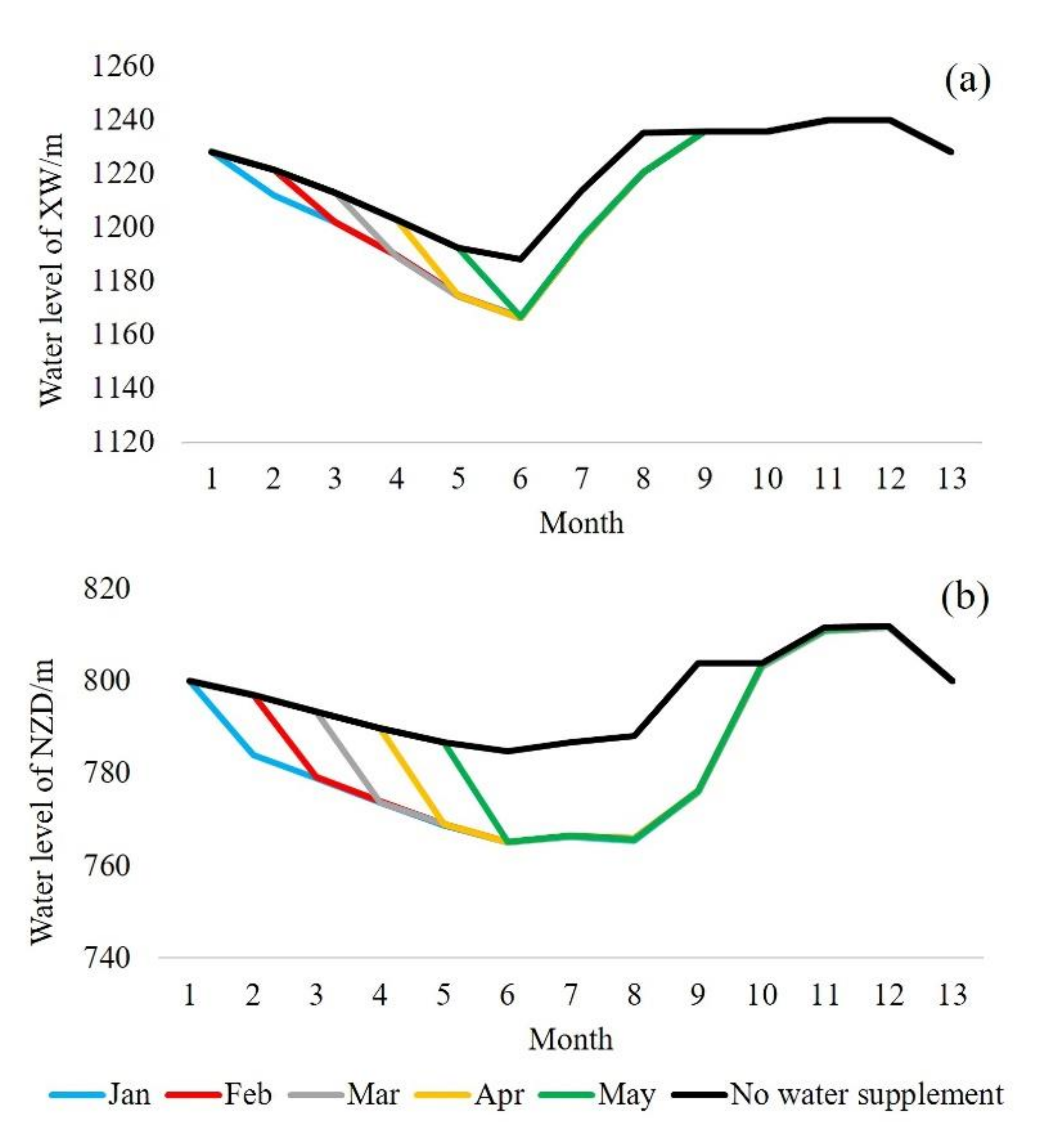
4.1. Limit State of Water Supplement

The ULF is related to the amount of inflow in the year, so the inflow processes of three typical hydrologic years are selected, which are 1997 (dry year, P = 75%), 1999 (normal year, P = 50%), and 2001 (wet year, P = 25%). The initial and final water level of the two hydropower stations adopt the average water level at the beginning of January of each year after the completion of the hydropower station; that is, the initial and final water levels of XW are 1228 m, and those of NZD are 800 m. In practical application, the initial and final water levels of the hydropower station can be determined according to the actual situation of that year. For each water supplement period of three typical years, the limit state of water supplement is calculated according to the method shown in 3.1, and the ULF is shown in Figure 5.

Figure 5 shows the ULF of each water supplement period in three typical years. As shown in Figure 5, the ULF increases significantly with the increase of inflow on the whole, which is easy to understand; more water brings greater regulation space under the constraints. When it comes to a specific year, in normal and wet years, the later the water supplement time, the higher the ULF, and one month’s delay will raise the ULF by about 5%. While in the dry year, the effect of delaying the water supplement time on the ULF is very weak.

Then, the ULF of each period of the years which are suitable for water supplement in the long series from 1978 to 2008 are plotted in Figure 6 (the year suitable for water supplement is the year in which the initial output process is a feasible output process). Among the 31 years from 1978 to 2008, there are 24 years when the initial output process is a feasible output process. The dotted lines from bottom to top are the regression lines of ULF from January to May. The ULF of each month decreases significantly with the decrease of inflow from the perspective of regression, and the regression lines also correspond to the conclusions of the ULF in typical years in Figure 5.

Due to the influence of annual inflow distribution, there is a large gap between the ULF and the regression line in some years, such as 1985 (P = 19%) and 2005 (P = 42%) which are circled by dotted lines. The annual average runoff of Lancang River Basin from January to May accounts for 19% of that of the whole year. However, in 1985, that proportion was 14%, and for 2005, the number was 22%. When the proportion is lower than the average, there is less inflow in the non-flood season and the water levels drop quickly during the period, so even in a wet year the ULF will be limited because the reservoir will run out of storage quickly. The same is true for 2005, and even in a normal year the ULF can be higher than some wet years because there is more water in the non-flood season.

Delaying the water supplement time can increase the ULF in normal and the wet years, which can be explained as follows: Taking 2001 (wet year, P = 25%) as an example, Figure 7 shows the water level processes of the reservoirs under limit states of water supplement in 2001, and different colors represent different water supplement time or no water supplement. As shown in Figure 7, the water level drops significantly in both reservoirs during the water supplement period compared to that of no water supplement (black line as indicated in the legend), leading to lower water heads and lower power generation efficiency after water supplement compared to that of no water supplement. According to the calculation of ULF, the output of each period is the firm power except the water supplement periods. With generation of the same firm power, periods with a high water head (level) use less water than those with a low water head (level), and so delaying the water supplement time can ensure more periods before the water supplement period have a higher water head (level) with a higher generation efficiency to save more water for the water supplement. In another word, the larger difference between the high water level before water supplement and the low water level after water supplement compared to that of no water supplement is the fundamental reason why delaying the water supplement time can improve ULF.

Thus, it is not difficult to understand that delaying the water supplement time has little effect on the ULF in dry years with the help of Figure 8 and Figure 9, which show the water level processes of XW and NZD under the limit state of water supplement in 1997 (dry year, P = 75%) and 1983 (dry year, P = 81%, the rightmost year in Figure 6). This is because the ULF in dry years is comparatively low already because of the overall low inflow, and the drop of water head (level) of the two reservoirs during the water supplement period is also slight, as shown in Figure 8 (1997). Sometimes, in some remarkable dry years, the water level of NZD at the end of the water supplement period is even higher than that of no water supplement under the limit state of water supplement, because it receives a large amount of discharge water from XW in the water supplement period, as shown in Figure 9 (1983).

Although the water levels of the two reservoirs changes greatly during the water supplement period in Figure 9, the ULF is not high because 1983 was a dry year. During the water supplement periods, plenty of water was only transferred from XW to NZD but not discharged to downstream from NZD. According to the fundamental reason why delaying the water supplement time can improve ULF, mentioned before, when the water level of one reservoir increases while that of the other one decreases during the water supplement period, the effect of delaying water supplement time on ULF will be not obvious with uncertainty.

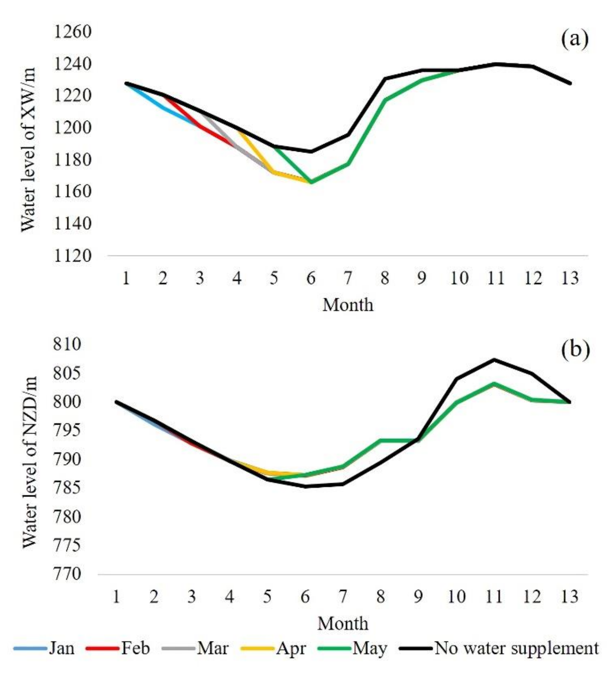
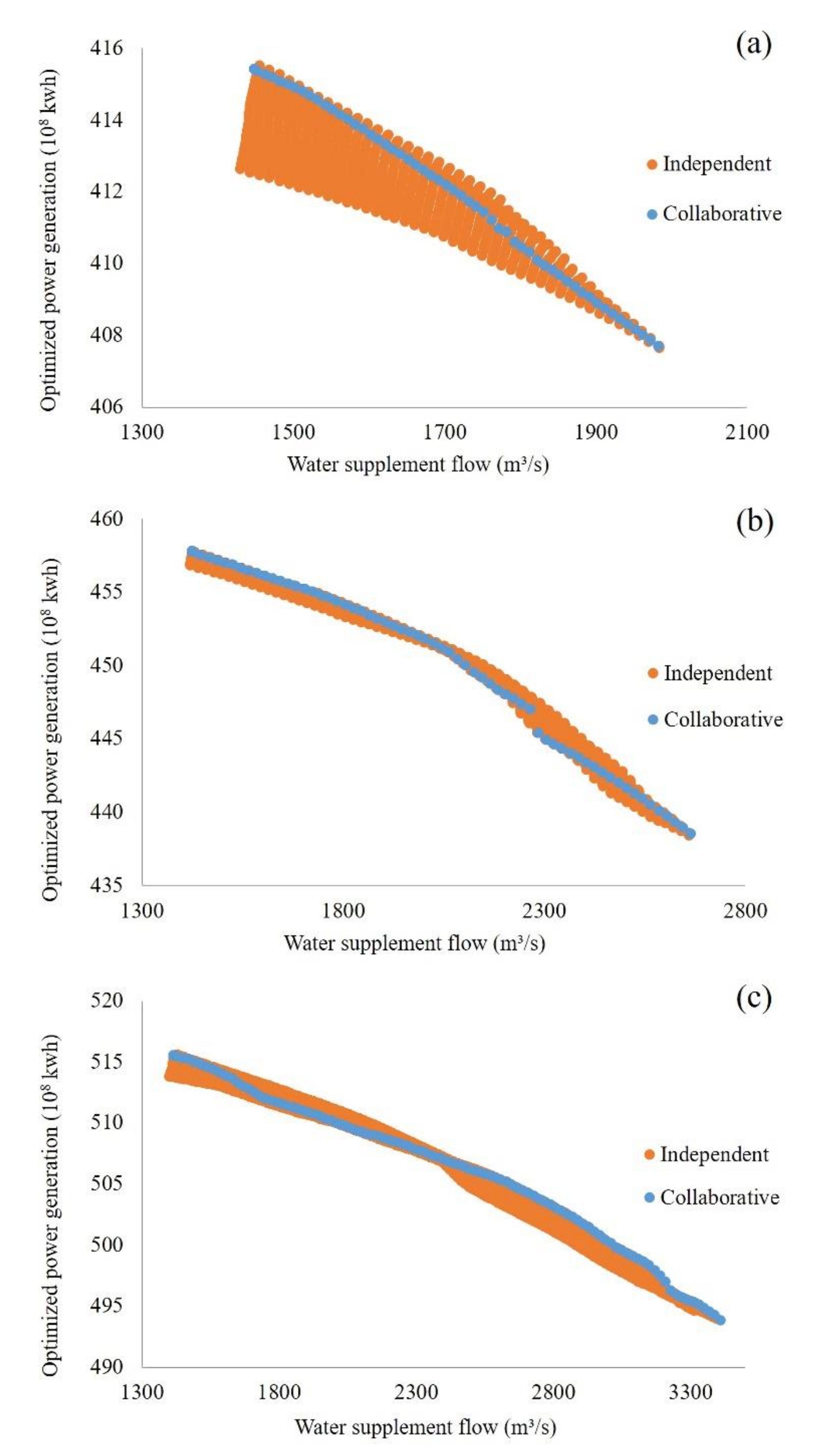
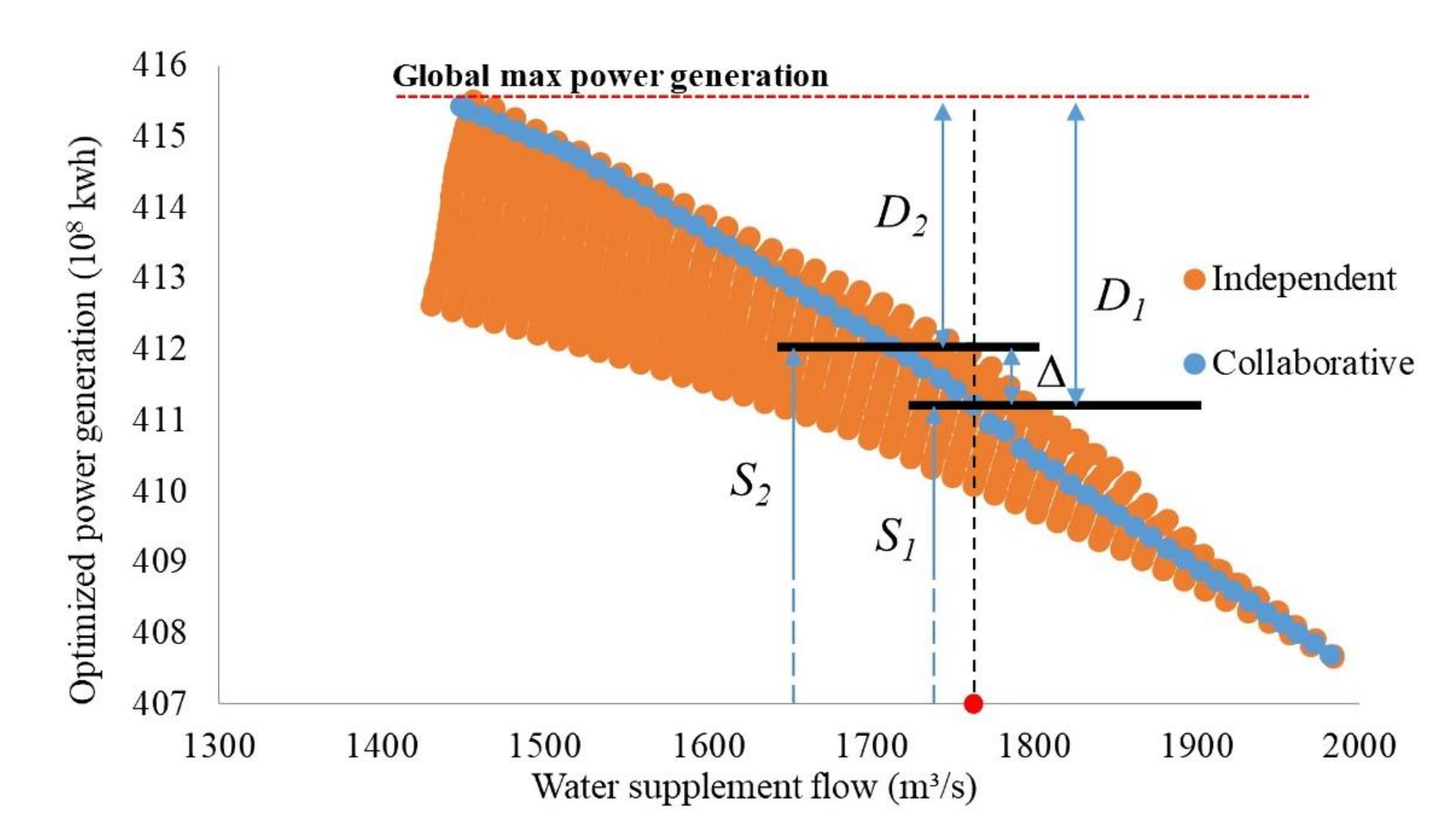
4.2. Effect Evaluation of “Collaborative Independent” Joint Optimization Method

The three typical years in 4.1 are also selected to calculate the “flow-energy” relationship and the PGL. In this paper, the dry season of each typical year is divided into five water supplement periods according to the month. The “flow-energy” relationship of 15 periods in three years can be obtained by the method in Section 3.2. Each group is composed of discrete points obtained by collaborative optimization and independent optimization. The discrete points in different periods have a similar pattern, so Figure 10 only shows the optimization results of three typical periods, in which the optimization results of “collaborative” and “independent” differs more obviously. The periods are April 1997 (a), March 1999 (b), and March 2001 (c).

As shown in Figure 10, the blue points are point cluster 1 (the result of collaborative optimization), and orange represents point cluster 2 (the result of independent optimization). The envelope curve formed by the points on the non-dominated layer of the two groups of points is the “flow-energy” relationship. In the scenarios studied above, the non-dominated layer of point cluster 1 and that of point cluster 2 dominate each other at different water supplement flows. For point cluster 1 and the non-dominated points of point cluster 2, it is shown that under some water supplement flows, the power generation of the latter can be visibly higher than the former. However, under some other water supplement flows, the power generation of the former is higher than the latter but only to a very slight extent, or is even nearly equal. Overall, the application of the two methods has improved the local optimum. Among them, the distribution of point cluster 2 has a certain “thickness” in the longitudinal direction. The existence of this “thickness” indicates that under the same water supplement flow of NZD, multiple maximum power generations can be obtained according to the independent optimization method. This is because of different allocations of the supplement water (or different combinations of the discharge flow) between the reservoirs during the water supplement period. Therefore, this “collaborative-independent” joint optimization method, on the premise of controlling the calculation time, considers the three thorny problems of cascade coordination, water supplement allocation, and local optimization as far as possible and finally obtains a satisfactory result. In the following, this paper makes a detailed comparison of the calculation results of the two optimization methods of the above three water replenishment periods to explore the improvement effect of the two optimization methods on the calculation results of power generation loss.

The PGL determines whether upstream and downstream cooperation in the Lancang-Mekong river basin can be achieved, which is the most critical value of concern for upstream and downstream countries. Therefore, the improvement percentage of power loss is used to evaluate the local optimal improvement effect of the two methods. Take April 1997 as an example (as shown in Figure 11); when the water supplement flow is 1770 m³/s (black vertical dotted line), the maximum power generation obtained by collaborative optimization is $S_1$. The corresponding generation loss is $D_1$. The maximum power generation obtained by independent optimization is $S_2$. The corresponding generation loss is $D_2$. Thus, the power generation difference of the two methods is $\Delta$, and the improvement ratio of the PGL caused by the application of the two methods is $p$:

$$p=\frac{\Delta }{max\left(D_1,D_2\right)}\times 100$$

(13)

Figure 12 shows the relationship between $p$ and water supplement flow in three scenarios of April 1997 (a), March 1999 (b), and March 2001 (c). When the water supplement flow is lower than 1500 m³/s), due to the fact that the water supplement flow is near the lower limit (flow that just meets the firm power constraint of NZD). Both $D_1$ and $D_2$ are very small, so the denominator in Equation (3) is also very small. In this case, the improvement percentage $p$ could be abnormally high. However, considering that the water supplement flow in this interval is nearly the same as the discharge flow that just meets the firm power, the water supplement would be of little significance. Therefore, only the intervals with large water supplement flow (>1500 m³/s) are analyzed. It can be seen that the “collaborative-independent” joint optimization method applied in this paper can significantly reduce the PGL, and the maximum improvement of PGL is about 18% in Figure 12a, about 16% in Figure 12b, and about 33% in Figure 12c when the water supplement flow is greater than 1500 m³/s. The improvement is significant enough to affect to water supplement cooperation so the method is meaningful and necessary.

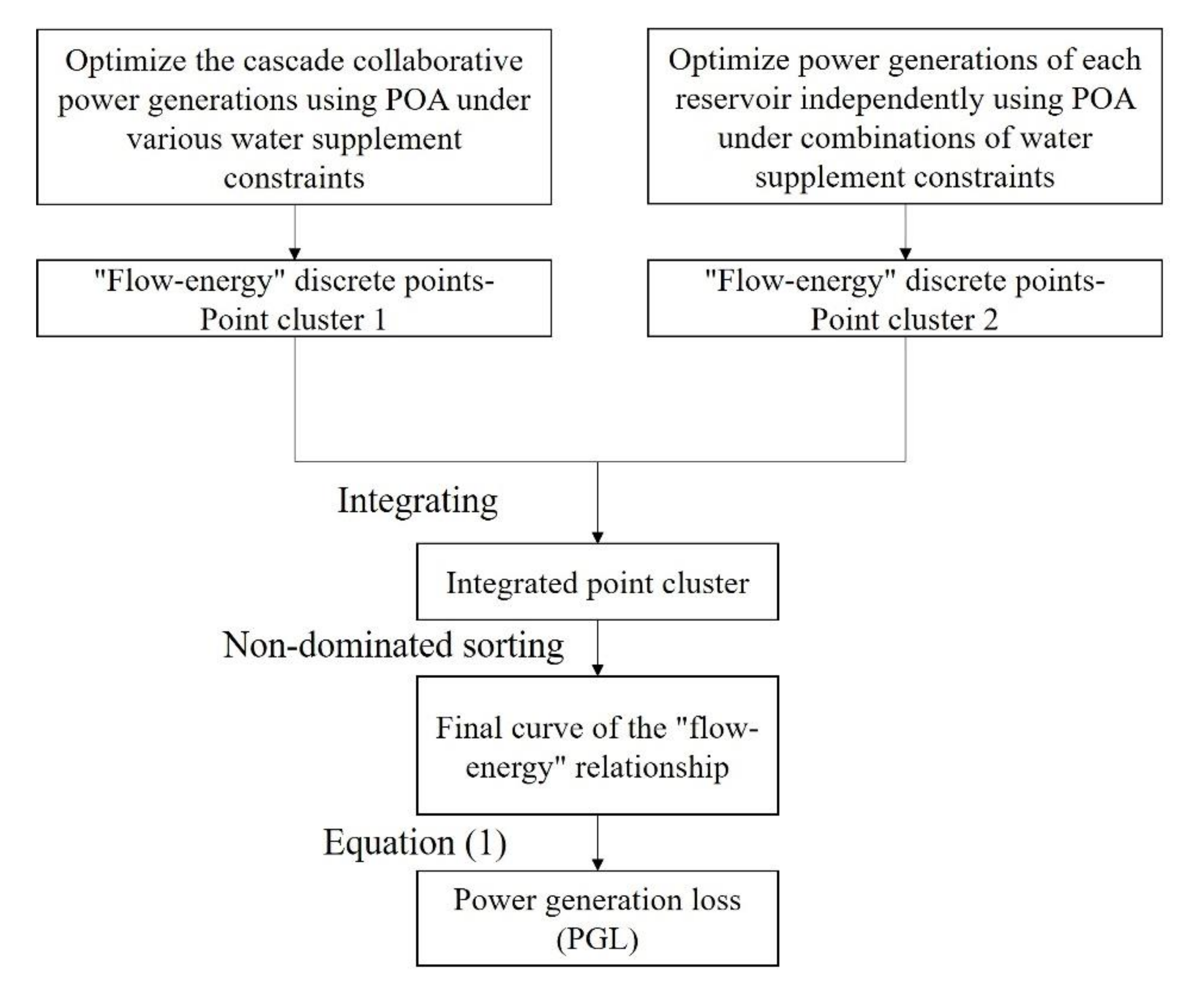
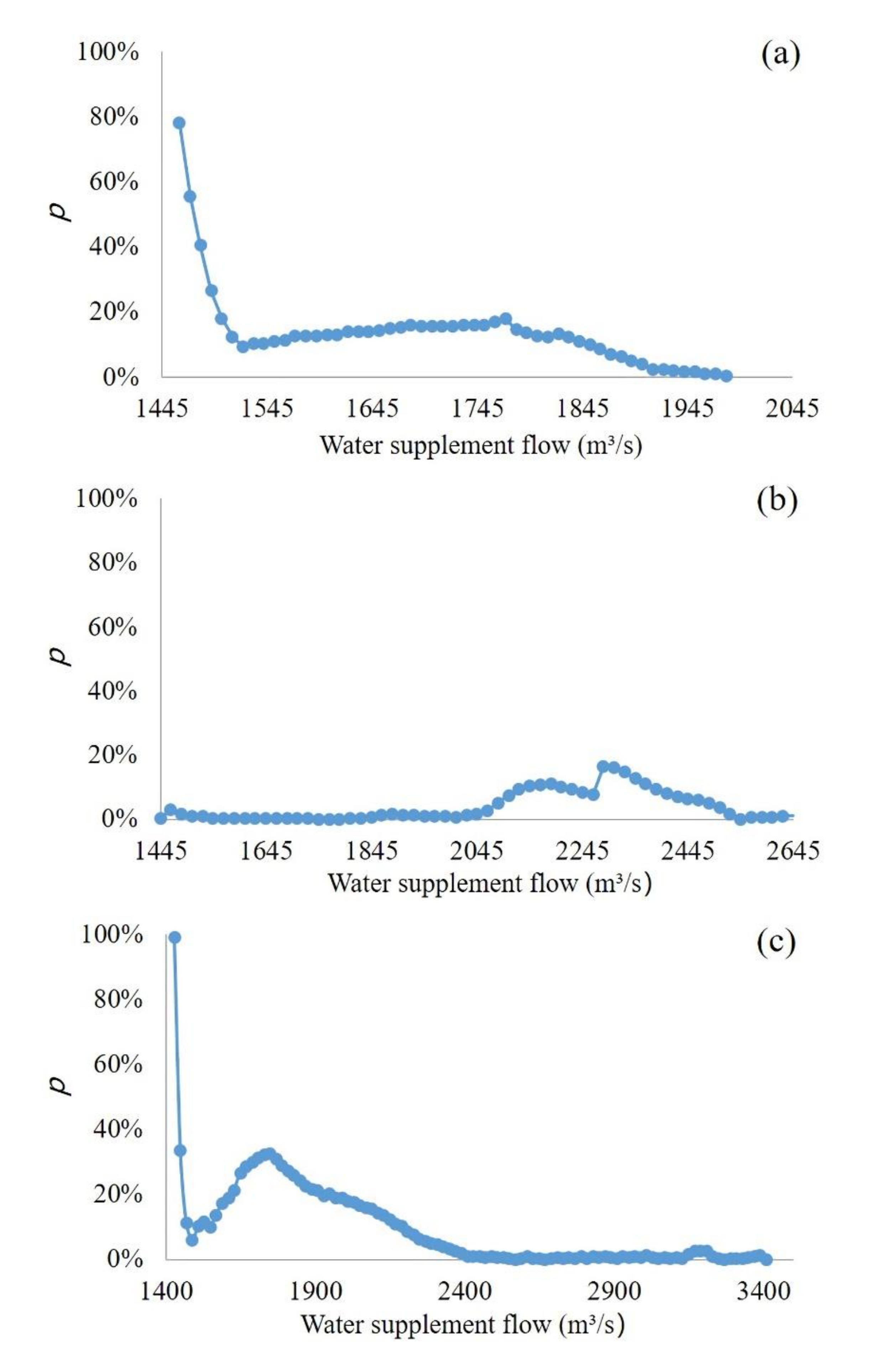
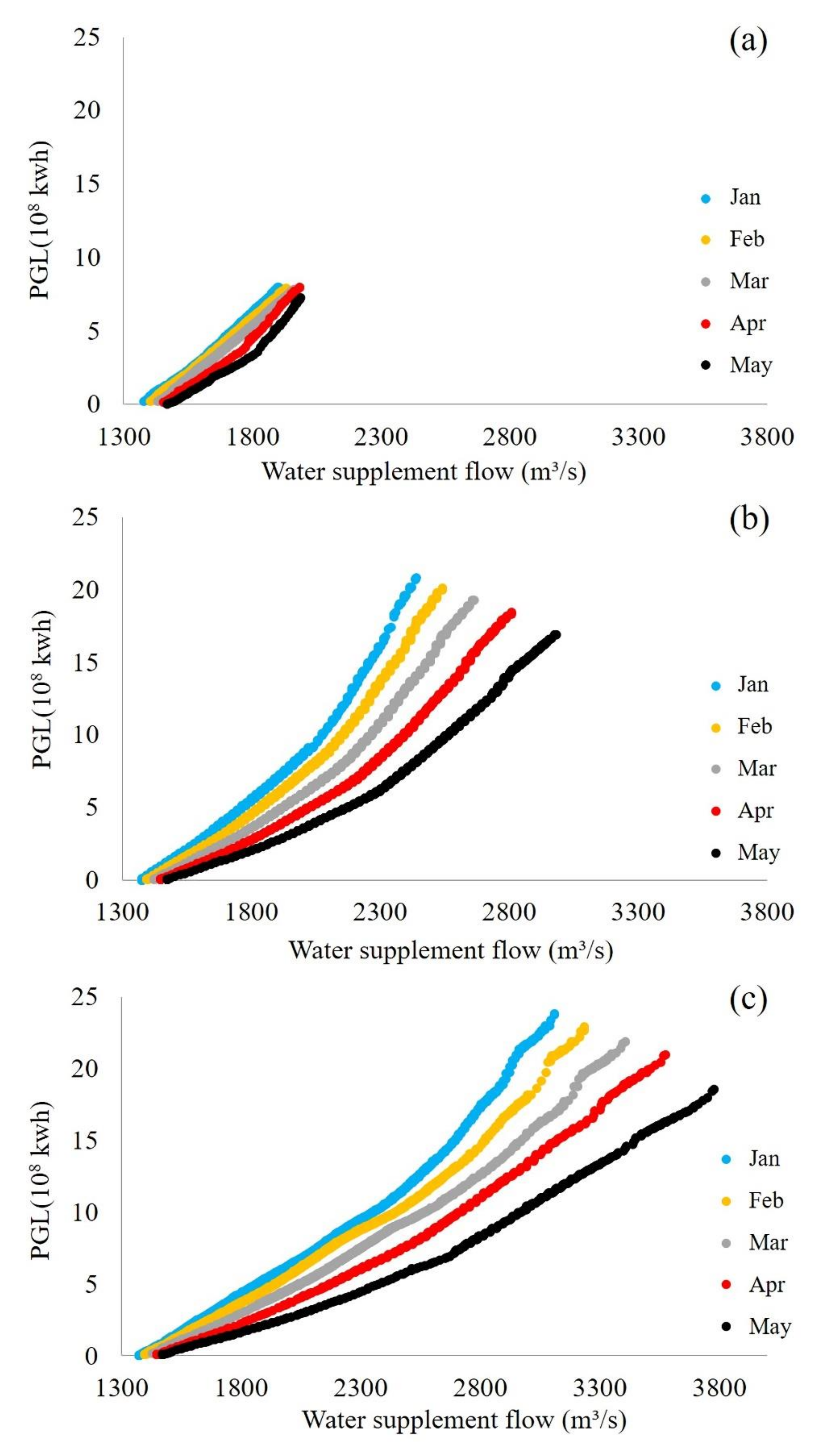
4.3. Power Generation Loss (PGL) of Water Supplement

The PGLs calculated by Equation (1) from the “flow-energy” relationship of all water supplement periods in the three typical years are plotted in Figure 13.

As shown in Figure 13, the PGL will increase with the increase of water supplement flow, and the three typical years have a similar pattern of PGL and the abscissa of the rightmost point of each line represents the corresponding ULF, which is consistent with the previous conclusion in 4.1. Under the same water supplement flow, the later the water supplement time is, the smaller the PGL is, so delaying the water supplement time can reduce the PGL. Accordingly, if the PGL is limited, delaying the water supplement time can increase the water supplement flow allowed. In addition, because each point in the point clusters is the optimal operating result, the operation process of each point in the non-dominated layer, including the water supplement allocation between the reservoirs during the water supplement period, can be obtained from the results. Therefore, these operation processes can be used to guide the operation. Taking March 1999 as an example, the scatter diagram of the discharge policy combinations of the two hydropower stations during the water supplement period is shown in Figure 14. The discharge combinations of the two hydropower stations during the water replenishment period should fall within the coverage of the point set in Figure 11 when facing different water supplement constraints in order to obtain a maximum power generation of minimum PGL under the water supplement constraint.

5. Discussion

Water supplement cooperation brings losses to the upstream and benefit increments to the downstream. Water supplement cooperation makes sense only when downstream benefit increment is greater than upstream losses so that the whole benefit of the basin will be improved after cooperation. Agricultural irrigation benefit is the most important interest of downstream countries, and it is closely related to water supplement time and the water shortage situation in that year. Sometimes, the agricultural benefit increment brought by water supplement in January is greater than that in May, but the upstream loss of water supplement in January is also greater than that in May, so downstream countries need to weigh the relationship among water supplement volume (flow), and water supplement time when applying for water supplement to make sure that their benefit increment is greater than the loss of upstream (PGL) to achieve the cooperation. Therefore, the ULF and PGL play important roles in deciding whether the cooperation should be achieved or not and have great research value.

When it comes to cooperation mechanism, the downstream beneficiaries must compensate the upstream power loss in a particular form so that both sides are willing to cooperate. If the compensation that downstream countries are willing to pay is more than the loss of the upstream, then the water supplement cooperation can enhance the water resources interests of the whole basin, and water supplement can ensure all countries in the basin achieve a win-win scenario; otherwise, the water supplement cooperation will be hard to achieve because the upstream countries see no benefit through the cooperation. As for how the beneficiary (downstream) should compensate the upstream and how much compensation should be made upstream, this can be decided through negotiation; that is, make the water supplement cooperation market-oriented to give full play to the decisive role of the market in resource allocation.

Additionally, different from the global optimization research [14,15] mentioned in the introduction, this modular form of water resource cooperation allows the upstream and downstream modules to focus on their own interests and the only thing that connects them is the negotiation. That means there are not too many complex objectives to be quantified and strategy variables to be optimized as in the global optimization research, so it is very efficient.

6. Conclusions

Based on the background of Lancang-Mekong water resources cooperation, taking the Lancang cascade hydropower stations in China as an example, this paper studies the ULF and PGL of water supplement in the non-flood season. First of all, this paper puts forward the calculation method of limit state of water supplement, so as to obtain the ULF in water supplement periods of different hydrologic years. Then, this paper also uses the “collaborative-independent” joint optimization method to optimize the power generation of cascade hydropower stations under the constraint of water supplement, obtains a more accurate “flow-energy” relationship than the solution of the traditional optimization methods, and taps the optimal allocation mode of supplement water between the reservoirs from the optimization results.

The results show that the ULF of each period will increase with the increase of water inflow in the year, but the distribution of the inflow within the year will also significantly affect the ULF. On the premise of similar total water inflow in the year, when the proportion of water inflow in non-flood season is higher than normal, the ULF will also be higher than average; otherwise it will be lower. In normal and wet years, the later the period of water supplement, the greater the ULF; The PGL increases with the increase of water supplement flow. Under the same water supplement flow, delaying the water supplement time can reduce the PGL. In addition, “collaborative optimization method“ and “independent optimization method“ show good complementarity, which is helpful to obtain more accurate PGL.

According to the analysis of this paper, water resources cooperation is meaningful and will bring overall benefit increment only when the benefits of downstream countries outweigh the loss of upstream power generation, so the existence of PGL can avoid ineffective water supplement cooperation and the conclusion of this paper can provide important data support for the negotiation of water supplement cooperation in Lancang Mekong River Basin in the future, and reasonably promote the achievement of Lancang-Mekong water resources cooperation and water resources utilization efficiency of the basin.

References

1. Ohlsson, L. Water conflicts and social resource scarcity. Phys. Chem. Earth Part B 2000, 25, 213–220. [Google Scholar] [CrossRef]
2. Dinar, S. Scarcity and Cooperation along International Rivers. Glob. Environ. Politi. 2009, 9, 109–135. [Google Scholar] [CrossRef]
3. Dinar, S.; Katz, D.; De Stefano, L.; Blankespoor, B. Do treaties matter? Climate change, water variability, and cooperation along transboundary river basins. Political Geogr. 2019, 69, 162–172. [Google Scholar] [CrossRef]
4. Dinar, S. Water, Security, Conflict, and Cooperation. SAIS Rev. 2002, 22, 229–253. [Google Scholar] [CrossRef]
5. Grey, D.; Sadoff, C. Beyond the river: The benefits of cooperation on international rivers. Water Sci. Technol. 2003, 47, 91–96. [Google Scholar] [CrossRef]
6. Huang, Z.; Liu, X.; Sun, S.; Tang, Y.; Yuan, X.; Tang, Q. Global assessment of future sectoral water scarcity under adaptive inner-basin water allocation measures. Sci. Total Environ. 2021, 783, 146973. [Google Scholar] [CrossRef]
7. Veilleux, J.; Dinar, S. A geospatial analysis of water-related risk to international security: An assessment of five countries. Geojournal 2021, 86, 185–238. [Google Scholar] [CrossRef]
8. Delbourg, E.; Dinar, S. The globalization of virtual water flows: Explaining trade patterns of a scarce resource. World Dev. 2020, 131, 104917. [Google Scholar] [CrossRef]
9. Xia, Q.; Qian, C.; Du, D.; Zhang, Y. Conflict or cooperation? How does precipitation change affect transboundary hydropolitics? J. Water Clim. Chang. 2021, 12, 1930–1943. [Google Scholar] [CrossRef]
10. Dinar, A.; Dinar, S.; McCaffrey, S.; McKinney, D. Bridges over Water: Understanding Transboundary Water Conflict, Negotiation and Cooperation. World Scientific Series on Energy and Resource Economics; World Scientific Publishing: Singapore, 2007; Volume 3. [Google Scholar]
11. Dinar, S.; Dinar, A.; Kurukulasuriya, P. Scarcity and Cooperation along International Rivers: An Empirical Assessment of Bilateral Treaties1. Int. Stud. Q. 2011, 55, 809–833. [Google Scholar] [CrossRef]
12. Wolf, A.T. Shared Waters: Conflict and Cooperation. Annu. Rev. Environ. Resour. 2007, 32, 241–269. [Google Scholar] [CrossRef] [Green Version]
13. MRC (Mekong River Commission). Mekong River Commission, China Discuss Joint Study. 2016. Available online: http://www.mrcmekong.org/news-and-events/events/mekong-river-commission-china-discuss-joint-study/ (accessed on 12 August 2021).
14. Yu, Y.; Zhao, J.; Li, D.; Wang, Z. Effects of hydrologic conditions and reservoir operation on transboundary coop-eration in the Lancang–Mekong River Basin. J. Water Resour. Plan. Manag. 2019, 145, 04019020. [Google Scholar] [CrossRef]
15. Li, D.; Zhao, J.; Govindaraju, R.S. Water benefits sharing under transboundary cooperation in the Lancang-Mekong River Basin. J. Hydrol. 2019, 577, 123989. [Google Scholar] [CrossRef]
16. Wheeler, K.G.; Hall, J.W.; Abdo, G.M.; Dadson, S.J.; Kasprzyk, J.R.; Smith, R.; Zagona, E.A. Exploring Cooperative Transboundary River Management Strategies for the Eastern Nile Basin. Water Resour. Res. 2018, 54, 9224–9254. [Google Scholar] [CrossRef]
17. Alemu. Dinar The Process of Negotiation Over International Water Disputes:The Case of the Nile Basin. Int. Negot. 2000, 5, 331–356. [Google Scholar] [CrossRef]
18. Li, D.; Long, D.; Zhao, J.; Lu, H.; Hong, Y. Observed changes in flow regimes in the Mekong River basin. J. Hydrol. 2017, 551, 217–232. [Google Scholar] [CrossRef]
19. Lund, J.R.; Guzman, J. Derived Operating Rules for Reservoirs in Series or in Parallel. J. Water Resour. Plan. Manag. 1999, 125, 143–153. [Google Scholar] [CrossRef] [Green Version]
20. Tao, F.; Jing, G.; Kong, K.; Yue, X.; Xiao, Z. Primary analysis of the loss of Longyangxia power station in abnormal water dispatch. J. Northwest Hydroelectr. Power 2019, 20, 5–8. (In Chinese) [Google Scholar]
21. Bellman, R.E.; Dreyfus, S.E. Applied Dynamic Programming; Princeton University Press: Princeton, NJ, USA, 1962. [Google Scholar]
22. Heidari, M.; Chow, V.T.; Kokotović, P.V.; Meredith, D.D. Discrete Differential Dynamic Programing Approach to Water Resources Systems Optimization. Water Resour. Res. 1971, 7, 273–282. [Google Scholar] [CrossRef]
23. Howson, H.R.; Sancho, N.G.F. A new algorithm for the solution of multi-state dynamic programming problems. Math. Program. 1975, 8, 104–116. [Google Scholar] [CrossRef]
24. Turgeon, A. Optimal short-term hydro scheduling from the principle of progressive optimality. Water Resour. Res. 1981, 17, 481–486. [Google Scholar] [CrossRef]
25. Larson, R.E.; Korsak, A.J. A new algorithm for the solution of multi-state dynamic programming problems. Auto-Matica 1970, 6, 245–260. [Google Scholar]
26. Yang, K.; Feng, J.; Lu, G. Study on convergence of the progressive optimality algorithm in reservoir operation. J. Hohai Univ. 1996, 24, 104–107. (In Chinese) [Google Scholar]
27. MRC (Mekong River Commission). State of the Basin Report; MRC: Vientiane, Laos, 2010. [Google Scholar]
28. Johnston, R.; Kummu, M. Water resource models in the Mekong Basin: A review. Water Resour. Manag. 2012, 26, 429–455. [Google Scholar] [CrossRef]
29. Li, S.; Bush, R.T. Rising flux of nutrients (C, N, P and Si) in the lower Mekong River. J. Hydrol. 2015, 530, 447–461. [Google Scholar] [CrossRef]
30. Zeng, Y.; Wu, X.; Cheng, C.; Wang, Y. Chance-Constrained Optimal Hedging Rules for Cascaded Hydropower Reservoirs. J. Water Resour. Plan. Manag. 2014, 140, 04014010. [Google Scholar] [CrossRef]
31. Tilt, B.; Gerkey, D. Dams and population displacement on China’s Upper Mekong River: Implications for social capital and social–ecological resilience. Glob. Environ. Chang. 2016, 36, 153–162. [Google Scholar] [CrossRef] [Green Version]
32. Chen, X.; Xu, B.; Zheng, Y.; Zhang, C. Nexus of water, energy and ecosystems in the upper Mekong River: A system analysis of phosphorus transport through cascade reservoirs. Sci. Total Environ. 2019, 671, 1179–1191. [Google Scholar] [CrossRef]
33. Deng, J.; Li, Y.; Xu, B.; Ding, W.; Zhou, H.; Schmidt, A. Ecological optimal operation of hydropower stations to max-imize total phosphorus export. J. Water Resour. Plan. Manag. 2020, 146, 04020075. [Google Scholar] [CrossRef]
34. Srinivas, N.; Deb, K. Multiobjective optimization using nondominated sorting in genetic algorithms. Evol. Comput. 1994, 2, 221–248. [Google Scholar] [CrossRef]
Figure 1. Overview of Lancang-Mekong River Basin.
Water 13 02826 g001
Figure 2. The calculation process of ULF.
Water 13 02826 g002
Figure 3. The discrete combinations of the output constraints in water supplement period.
Water 13 02826 g003
Figure 4. The calculation of process of “flow-energy” relationship and PGL using the “collaborative-independent” joint optimization method.
Water 13 02826 g004
Figure 5. The ULFs in typical years of wet, normal and dry year.
Water 13 02826 g005
Figure 6. The ULF pattern of all hydrological years.
Water 13 02826 g006
Figure 7. The water level processes of XW (a) and NZD (b) under the limit state of water supplement in 2001 (wet year, P = 25%).
Water 13 02826 g007
Figure 8. The water level processes of XW (a) and NZD (b) under the limit state of water supplement in 1997 (dry year, P = 75%).
Water 13 02826 g008
Figure 9. The water level processes of XW (a) and NZD (b) under the limit state of water supplement in 1983 (dry year, P = 81%).
Water 13 02826 g009
Figure 10. Optimization results of “flow-energy” relationship under “collaborative-independent” joint optimization. (a) April 1997, (b) March 1999, and (c) March 2001.
Water 13 02826 g010
Figure 11. Effect evaluation method of “collaborative independent” joint optimization.
Water 13 02826 g011
Figure 12. Effect evaluation of “collaborative independent” joint optimization. (a) April 1997, (b) March 1999, (c) March 2001.
Water 13 02826 g012
Figure 13. Results of PGL of the three typical years, (a) Dry year, P = 75%; (b) normal year, P = 50%; and (c) wet year, P = 25%.
Water 13 02826 g013
Figure 14. Optimized strategy combinations of hydropower stations during water supplement period (water supplement in March 1999).
Water 13 02826 g014