
Investigating Controls on Barrier Island Overwash and Evolution during Extreme Storms


1
Department of Earth and Ocean Sciences, University of North Carolina Wilmington, Wilmington, NC 28403, USA
2
Department of Physics and Physical Oceanography, University of North Carolina Wilmington, Wilmington, NC 28403, USA
*
Author to whom correspondence should be addressed.
Water 2021, 13(20), 2829; https://doi.org/10.3390/w13202829
Submission received: 23 September 2021
/
Revised: 6 October 2021
/
Accepted: 8 October 2021
/
Published: 12 October 2021
(This article belongs to the Special Issue Wave-Driven Processes in the Coastal Zones)
Abstract
:Over short periods of time, extreme storms can significantly alter barrier island morphology, increasing the vulnerability of coastal habitats and communities relative to future storms. These impacts are complex and the result of interactions between oceanographic conditions and the geomorphic, geological, and ecological characteristics of the island. A 2D XBeach model was developed and compared to observations in order to study these interactions along an undeveloped barrier island near the landfall of Hurricane Florence in 2018. Beachface water levels during the storm were obtained from two cross-shore arrays of pressure sensors for comparison to model hydrodynamics. Aerial drone imagery was used to derive pre-storm and post-storm elevation data in order to quantify spatially varying erosion and overwash. Sediment grain size was measured in multiple locations, and we estimated spatially varying friction by using Sentinel-2 satellite imagery. The high spatial and temporal resolution of satellite imagery provided an efficient method for incorporating pre-storm spatially varying land cover. While previous studies have focused on the use of spatially varying friction, we found that the utilization of local median grain sizes and full directional wave spectra was critical to reproducing observed overwash extent.
1. Introduction
Prominent coastal features around the world such as barrier islands provide substantial value to surrounding areas through ecosystem and protective services (e.g., habitat for threatened species and buffer mainland areas from wave energy [1]) and economic opportunities (e.g., recreation and tourism [2]). However, these benefits are highly dynamic and are based on changes in barrier island morphology that occur over a wide range of temporal and spatial scales, with changes driven by natural and anthropogenic causes [3]. Despite this dynamic nature, many barrier islands have become heavily developed and densely populated over the past century [4,5]. Growing coastal populations and tourism demands have necessitated the protection of coastal resources and infrastructure [2,6] from impacts associated with changing oceanographic forcings including extreme storms and relative sea-level rise (RLSR). While they lack infrastructure, undeveloped barrier islands are also influenced by coastal engineering practices of adjacent coastal areas (e.g., hard structures limiting longshore sediment transport, inlet dredging, etc.). These management actions may change the vulnerability of particular areas or habitats along a barrier island necessitating the development of tools for use by coastal managers to guide decisions and potentially increase island resiliency.
Storm events, in particular, are significant contributors to the landward transport of sediment through overwash and breaching associated with coastal inundation [7,8] that can remove sediment from the nearshore system and drive island rollover. The response of a barrier island to an individual storm event is primarily influenced by the pre-storm morphology and the magnitude and duration of time-varying total water levels (TWL; a combination of astronomical tide, storm surge, and wave runup) throughout a storm [8,9]. Cumulative impacts from inter-annual or intra-annual storms also influence longer-term barrier island migration [10], and the combined impacts of RSLR and potential increased storminess may cause barrier islands to drown on decadal timescales in the future [11]. For coastal decision makers, modeling approaches that can robustly quantify individual or repeated storm-driven sediment transport are essential to developing proper mitigation strategies (e.g., sand placements, retreat, and adaptation). One-dimensional (1D) cross-shore profile models of storm-driven hydrodynamics and dune evolution are computationally efficient and can provide reasonable estimates of how sections of a barrier island may respond to a storm (e.g., quantify cross-shore sediment transport, elevation changes to dunes, etc.). However, these models must be applied to sections of barrier islands that are relatively uniform alongshore [12] and have been found to provide different predictions compared to two-dimensional (2D) models that account for alongshore processes [9,13,14]. The implementation of 2D models can provide improved estimates of how an entire barrier island might respond to a storm event while taking into account alongshore variability in island elevation and hydrodynamic forcings.
XBeach [15] is one of the most widely developed and applied 2D models for hydrodynamic and morphodynamic processes on barrier islands during storms. Multiple studies have shown that XBeach can accurately simulate storm-induced dune erosion, overwash, and sediment transport driven by elevated waves and water levels [12,16,17,18], but there remains some uncertainty in the ability to accurately predict wave runup processes [19], and studies that quantify the accuracy of modeled overwash distances are limited [20,21]. XBeach model performance is typically validated using comparisons of pre-storm and post-storm elevation data while the accuracy of modeled hydrodynamics is inferred. Determining if errors between observed and modeled morphological changes are the result of inaccurate model physics (e.g., wave runup), poor specification of spectral wave or water level inputs at the model boundaries, or ignoring spatially varying geomorphological island characteristics (e.g., grain size and land cover) requires synoptic measurements that are challenging to collect during extreme storm events (e.g., Sherwood et al. [17]).
Previous studies found that XBeach overestimates erosion during overwash which was hypothesized to be a result of large velocities associated with sheet flow conditions [16,22]. A sediment transport limiter that maintains a constant equilibrium sediment concentration under sheet flow conditions was implemented to prescribe a linear relationship between sheet flow velocity and sediment transport [16]. However, in practice, this single parameter serves as a proxy for unknown and/or unrepresented processes during overwash conditions. Offshore wave and water level conditions were highly parameterized due to a lack of observations, and the amount of error introduced by these boundary conditions compared to unknown processes is unclear. Passeri et al. [18] found that using spatially varying Chezy coefficients calculated from land cover classifications eliminated the need for the sheet flow sediment transport limiter. The spatially varying friction caused vegetated areas in XBeach to have lower bed shear stress values, resulting in reduced cross-shore sediment transport during periods of overland flow.
Spatially varying friction coefficients in previous studies have been based on satellite and aerial imagery in coastal environments. Land cover classifications used by Passeri et al. [18] were obtained from the Coastal Change Analysis Program (C-CAP). C-CAP is a publicly available land cover dataset derived from satellite imagery. Similarly, Johnson et al. [21] used Landsat 5 imagery to compute spatially varying friction coefficients prior to Hurricane Gustav’s landfall in 2008. Both products have low spatial resolutions (30 m) that limit their applicability in barrier island environments. For instance, transitions from the beachface to dune and backbarrier environment are difficult to distinguish with 30 m cross-shore resolution. Additionally, C-CAP is updated on 5-year intervals and will not account for changes in land cover on shorter time scales. Other remote sensing data such as aerial imagery can also be used to derive estimates of spatially varying friction coefficients. van der Lugt et al. [23] derived land cover classifications from pre-storm National Agricultural Imagery Program (NAIP) aerial imagery with a 1 m spatial resolution, but the temporal and spatial availability of the imagery varies by region causing inconsistent coverage of different barrier islands over time. Modern satellites such as Sentinel-2 can capture land cover data at both high spatial and temporal resolutions (10 m and 2–3 days, respectively, for Sentinel-2 [24]) and provide a method to update land cover between modeled storm events in order to evaluate cumulative storm impacts.
While past XBeach studies have focused on applying spatially varying friction coefficients derived from land cover classifications to improve model performance, model sensitivity to changes in sediment grain size and specifically studies that quantify the skill of XBeach modeled overwash distances are limited. Using a 1D XBeach model, Koktas [25] determined that using representative grain sizes was important for modeling coastal morphodynamics in the nearshore region and beachface. Matias et al. [26] recently recorded shallow overwash events by using a video camera, pressure transducer, and current meter along a single cross-shore transect and examined the sensitivity of modeled overwash in a non-hydrostatic (wave-resolving) 1D XBeach model relative to different factors (wave height, lagoon water levels, nearshore topography, and grain size) and found that finer non-cohesive grain sizes increased the occurrence of overwash. Currently, studies have not focused on the accuracy of modeled overwash deposits using a 2D XBeach model applied at the barrier island scale. Studies at this scale have also not evaluated the individual roles of spatially varying friction coefficients, grain size, and offshore wave boundary conditions in accurately predicting storm-driven morphological changes.
The main objectives of this study are to use a 2D XBeach model at the barrier island scale to investigate the influence of morphodynamic (bed friction and grain sizes) and hydrodynamic (bulk vs. measured directional wave spectra) conditions on modeled elevation change and overwash extent. The sensitivity of modeled overwash extent is explored with regards to changes in grain size and the use of spatially varying friction coefficients computed from land cover classifications performed on high spatial and temporal resolution satellite imagery. Beachface water level sensors provide measurements of the timing and magnitude of TWL during a category one hurricane, allowing for comparisons between measured and modeled shoreface water levels for simulations using different hydrodynamic forcings. We assess the individual and combined impact of wave boundary conditions, grain size, and landcover in order to quantify the role each plays in elevation change and modeled overwash processes.
2. Materials and Methods
2.1. Study Site
Masonboro Island is a 13 km long undeveloped barrier island located off the coast of New Hanover County in southeastern North Carolina and part of the National Estuarine Research Reserve system (Figure 1 [27]). The island supports a variety of coastal and estuarine species, including some designated as threatened (e.g., loggerhead and green sea turtles and seabeach amaranth) or species of concern (e.g., American oystercatcher and Wilson’s plover [27]). Masonboro Island currently experiences a sediment deficit due to a dual jetty system bounding Masonboro Inlet at the north end adjacent to Wrightsville Beach that was completed in 1981 and an inlet dredging at the north and south (Carolina Beach Inlet) ends of the island [28]. Six sand placements have occurred between 1986 and 2010, all conducted at the north end as sediment was dredged from Masonboro Inlet [2]. These anthropogenic activities have contributed to a diverse topography on Masonboro Island. The northern section has a well-developed, alongshore continuous dune system (average maximum pre-Hurricane Florence height of 4.4 m) and wider beaches due to an up-drift accretionary fillet against the adjacent jetty. The central section has lower dunes (average maximum pre-Hurricane Florence height of 3.1 m) and relatively narrow beaches. The southern section has small dunes (average maximum pre-Florence height 2.9 m) and variable beach widths that are narrower towards the center section and progressively wider moving towards the southern terminus at Carolina Beach Inlet. The different sections of the island are shown in Figure 2. Historically, cycles of extensive overwash at some locations and subsequent dune recovery have been recorded on Masonboro Island [29]. Lacking sand placements and stabilization from a jetty, the lower relief central and southern sections are more susceptible to overwash from extreme storms [27]. Using tide gauge-derived rates, Masonboro Island is expected to experience an increase in relative sea level of at least 6.1 cm by the year 2045, which will make the island more vulnerable to extreme morphological changes in the future [30].
Hurricane Florence made landfall along North Carolina’s southeastern coast as a category 1 hurricane (based on Saffir–Simpson Hurricane Wind Scale) on the morning of 14 September 2018 [32]. Maximum sustained wind speeds reached 102 km/h at Johnnie Mercer Pier in Wrightsville Beach, NC, resulting in a maximum storm tide (water level due to combined storm surge and astronomical tide) of 1.79 m (referenced to NAVD88 [32]), the highest water level recorded at this site since gauge installation in 2004 (previous high of 1.40 m, NAVD88). A wave buoy located 9.6 km offshore of Masonboro Island in ~15 m of water depth recorded a maximum significant wave height of 5.1 m (ILM2 wave buoy operated by the Coastal Ocean Research Monitoring Program; CORMP). Significant wave heights recorded by the ILM2 wave buoy exceeded 3 m for 54.5 h, and the measured water levels from the Wrightsville Beach NOAA tide station (Station ID: 8658163) exceeded mean higher high water (0.526 m, NAVD88) for 42 h. Masonboro Island experienced overwash in portions of the central and southern sections and extensive dune erosion in the northern section [32].
2.2. Model Description
XBeach solves coupled hydrodynamic and morphodynamic equations to model the storm-driven evolution of coastal areas, specifically incorporating wave runup on the beachface which is a primary driver of dune erosion and overwash during storms [15]. Validated for a variety of locations and storm conditions [11,12,13,15,16,19], XBeach can compute infragravity wave propagation, sediment transport, and bed level changes in the alongshore and cross-shore directions. We used the ‘surfbeat’ wave model option in XBeach (version 5526) which averages short-wave variations, resolving wave-groups and the associated infragravity waves. During periods with elevated wave heights (e.g., extreme storms), incident band swash becomes saturated, and infragravity band swash dominates driving alongshore and cross-shore currents and is the primary driver for dune erosion and overwash [15,33,34]. Given the inputs of time-varying water level boundary conditions (e.g., tides/surge) and short-wave frequency-direction spectra, XBeach simulates wave transformation and dissipation in the surf zone and the development of cross-shore and alongshore currents that initiate sediment motion when a critical combined wave-current shear stress is exceeded for a specified sediment density and size. Sediment transport is modeled using a depth-averaged advection-diffusion scheme where differences between the modeled sediment concentration in the water column and equilibrium concentration determine whether sediment is entrained or deposited [15].
XBeach is capable of modeling sediment transport for each of the storm-impact regimes outlined by Sallenger [8]. In the swash regime, the mass flux of waves and resulting return flow drives the erosion of the beachface transporting sediment offshore. For the collision regime, an avalanching model is used where infragravity waves wet the duneface, and if a critical bed slope is exceeded for wet or dry points, the duneface slumps. XBeach models the overwash regime by using a momentum-conserving drying/flooding formulation [35] where the occurrence of dune overtopping by infragravity waves results in a landward momentum flux and associated sediment transport. Persistent overwash can result in inundation and island breaching that XBeach simulates using a combination of avalanche-triggered bank erosion and sediment transport by channel flows.
2.3. Model Domain
The Masonboro Island XBeach model domain has variable cross-shore spacing (25 m offshore and decreasing to 3 m across the island) and constant 25 m alongshore spacing. Alongshore, the XBeach model domain encompasses the majority of Masonboro Island, excluding the northern and southern tips. Cross-shore, the XBeach domain extends from the 15 m offshore depth contour and across the subaerial island into the intracoastal waterway. Portions of the backbarrier marsh-filled lagoon are excluded. The bathymetric surface of the model domain comprises two continuously updated digital elevation models (CUDEM [36,37]), a 1/3rd arc-second resolution CUDEM extending from ~15 m water depth at the offshore boundary to ~13 m water depth, and a 1/9th arc-second resolution CUDEM extending from ~13 m water depth to the nearshore region of about ~1 m water depth. Information on the elevation data comprising the CUDEMs and development procedures is available in Amante et al. [38]. No pre-Florence bathymetric data from hydrographic measurements were available.
Pre-storm elevations between ~1 m water depth on the open ocean coastline to the back-barrier marsh comprised of drone-based digital elevation models (DEM [39]) where available merged with a 2017 U.S. Army Corps of Engineers (USACE) topo-bathymetric LiDAR DEM. The drone-derived DEMs were developed using structure-from-motion techniques applied to imagery collected with a fixed wing eBee GPS-equipped drone. Fixed-wing drones provide assessments of barrier island scales due to their increased flight efficiency. The post-storm elevation dataset used for analyses was generated from drone-based DEMs [39] merged with a post-Florence topo-bathymetric LiDAR dataset. Bathymetric and subaerial island elevation data were interpolated to the model grid separately then merged. Where two elevation data sets met, an average of the two touching grid points was used. The collection dates, spatial resolutions, and reported vertical accuracies of the elevation datasets used are shown in Table 1.
At the north and south ends of Masonboro Island, pre-storm and post-storm shore-normal elevation transects were collected using an RTK-GPS. These data were used to verify the elevation datasets used to develop the model grid. An altitude vertical offset was identified and corrected for at the south end between the post-storm elevation survey and both the drone DEM and topo-bathymetric LiDAR (biases of −0.11 m and 0.11 m, respectively). After correcting offsets, comparisons were made between the drone DEMs and topo-bathymetric LiDAR datasets to quantify the agreement between the merged datasets, particularly for the pre-storm topo-bathymetric LiDAR as it was collected a year before the storm. At the north end, pre-storm datasets had an RSME and bias of 0.19 m and −0.04 m, respectively, and post-storm datasets had an RMSE and bias of 0.17 m and −0.08 m, respectively. At the south end, pre-storm datasets had an RSME and bias of 0.22 m and 0.03 m, respectively, and post-storm datasets had an RMSE and bias of 0.14 m and −0.10 m, respectively.
2.4. Model Hydrodynamics
The model simulation spanned from 00:00 UTC 13 September 2018 to 00:00 UTC 17 September 2018. Wave data forced at the offshore boundary were obtained from the ILM2 wave buoy. Simulations were completed using both Joint North Sea Wave Project (JONSWAP [40]) spectra based on bulk wave characteristics, and observed variance density spectra were calculated using the maximum entropy method [41]. Wave boundary conditions were updated every 30 min and prescribed as a spatially uniform condition along the offshore boundary. Water levels forced at the offshore boundary were obtained from the Wrightsville Beach NOAA tide station just north (4.7 km) of the model domain. While sound side water levels were not measured during the storm, comparisons were made relative to two nearby water level stations during other time periods in order to assess a potential delay in sound side tide levels. These stations were the oceanside Wrightsville Beach NOAA tide station and a water level sensor at the UNCW Center for Marine Science dock behind Masonboro Island. A Gaussian process regression model was fit to water level sensor data on the sound side of Masonboro Island and data from the NOAA tide station. A 1 h delay was found between the sound side water levels and the NOAA tide station, hence, water levels were forced along the sound side boundary using the oceanside water levels delayed by 1 h. Before Hurricane Florence, cross-shore transects of water level sensors (HOBO® U20L-04 Data Logger with a 20-s sampling rate) were deployed at the bed level surface at the north and south ends (same locations as walking RTK-GPS transects) of Masonboro Island to record the timing and duration of beachface and dune water levels during the storm (Figure 2). The atmospheric pressure recorded by the Wrightsville Beach NOAA tide station during the storm was subtracted from the values recorded by the pressure sensors. Recorded beachface water levels were used to test the accuracy of simulated shoreface water levels.
2.5. Geomorphology
Four pre-storm sediment samples were collected at each of the four water level sensor locations at the north and south transects. Averaged measured D50 and D90 grain sizes at the north were 240 µm and 370 µm, respectively. Average measured D50 and D90 grain sizes at the south were 360 µm and 890 µm, respectively. For model input, the grain size values at the north and south were averaged, resulting in D50 and D90 grain size values of 300 µm and 630 µm, respectively. The measured grain sizes, particularly D90, are larger than the default values (D50 = 200 µm and D90 = 300 µm).
A supervised land cover classification (variation of the maximum likelihood classification process) was conducted in ArcMap on pre-Florence Sentinel-2 satellite imagery acquired on 8 September 2018 (Figure 3). The Copernicus Sentinel-2 mission has two polar-orbiting satellites in a sun-synchronous orbit resulting in a revisit time of 2–3 days at mid-latitudes under cloud-free conditions [24]. Sentinel-2 has 13 spectral bands: four bands at 10 m, six bands at 20 m, and three bands at 60 m spatial resolution [24]. Five land cover classes were extracted: open water, unconsolidated shore, grassland/herbaceous, estuarine emergent wetland, and deciduous forest. The pixel count for each training sample class is shown in Table 2. Due to the fact that no ground-truth points were available, a validation dataset was created using a random sample of 315 pixels from the satellite imagery by manually classifying land cover type. Statistics between the validation dataset and the classified map were computed using the compute confusion matrix tool in ArcMap (Table 3). A kappa index of agreement (0.80) was found between the supervised land cover classification and validation dataset. Excluding open water, each land cover class from the land cover classification was assigned a Manning’s n coefficient based on Dietrich et al. [42], which was converted to a Chezy coefficient assuming a 1 m flood depth over land. Open water Chezy coefficients for all simulations were depth-dependent and ranged from 31 to 71 m1/2/s.
2.6. Simulations Completed and Model Accuracy
Five major simulations were completed during model development by varying the input sediment grain size (default vs. measured), friction values (constant vs. spatially varying), and spectral wave boundary conditions (measured variance density vs. parameterized JONSWAP spectra). A list of the simulations completed is summarized in Table 4. Chezy coefficients for simulations using constant friction over land were set to 33 m1/2/s (equivalent to bare land).
Model accuracy was quantified by calculating the bias, RMSE, and coefficient of determination (r2) between modeled and measured bed level changes. These statistics were calculated for the entire island and separately for the northern, central, and southern sections of the island. The bias was calculated as follows:
where zb is the bed elevation. RMSE was calculated between modeled and measured bed level changes with the following equation:
where dzb is the elevation change.
In addition to the statistics of model accuracy for elevation changes, the cross-shore extent of overwash deposits that can damage coastal infrastructure and alter habitats during storm events [43] was also examined. High quality National Geodetic Survey (NGS) post-Florence imagery (ground sample distance of 15 cm [44]) was used to define a ~3.9 km long alongshore section containing visible continuous overwash for comparisons with the simulations. Using pre-Florence imagery as a reference, observed cross-shore overwash distances were digitized from the imagery in MATLAB. The distance from the 0 m pre-storm contour to the landward extent of apparent new sand in the back-barrier region of the island at each alongshore position in the model was determined. Similar comparisons were made between overwash from the default simulation and the other simulations. A polygon was drawn around the modeled overwash for each simulation covering the same alongshore extent. The cross-shore range of each polygon extended from the 0 m pre-storm contour to the landward extent of overwash, or if overwash was absent, to the limit of dune erosion. Overwash extent values for cross-shore transects with no overwash were set to 0 m.
Further analyses were completed by comparing changes to foredune crest elevation and volume from the baseline simulation and post-Florence elevation data. The foredune crest elevation for each cross-shore transect was defined as the first local topographic maximum landward of the shoreline. Foredune volume was calculated for each transect from the dune base to the dune heel (e.g., landward extent of the dune). The dune base was defined based on the maximum slope change between the dune crest and ocean shoreline. The dune heel was defined similarly but was confined between the dune crest and the first local topographic minimum landward of the dune crest.
Modified versions of Equations (1) and (2) above were used to calculate the bias and RMSE between measured and modeled overwash extents, measured and modeled post-Florence foredune crests and foredune volumes, and measured and modeled beachface water levels for the baseline simulation and the JONSWAP simulation. In each case, the measured values were subtracted from the modeled values (same as in Equations (1) and (2)).
3. Results
3.1. Beachface Water Levels
Comparisons between measured and modeled beachface water levels for the baseline simulation (defined in Table 4), and the simulations using parameterized bulk wave spectra are shown in Figure 4. During peak storm surge, modeled beachface water levels for the baseline simulation agreed well with observed beachface water levels at the northern transect (RMSE and bias of 0.104 m and −0.004 m, respectively). At the south end, the model overpredicted beachface water levels at S1 (RMSE and bias of 0.263 m and 0.182 m, respectively). The model predicted up to 25 cm of water at the S2 sensor, but the observations indicate only a few episodic pulses of water at the sensor with magnitudes less than 20 cm (RMSE and bias of 0.074 m and 0.026 m, respectively). Note that the output model time series at the sensor locations was equivalent to the sensor sampling rate. For the simulation using JONSWAP spectra as inputs, the model overpredicted beachface water levels at the north (RMSE and bias of 0.152 m and 0.052 m, respectively) and south ends (RMSE and bias of 0.334 m and 0.279 m, respectively, for S1 and RMSE and bias of 0.103 m and 0.050 m, respectively, for S2).
3.2. Bed Level Changes
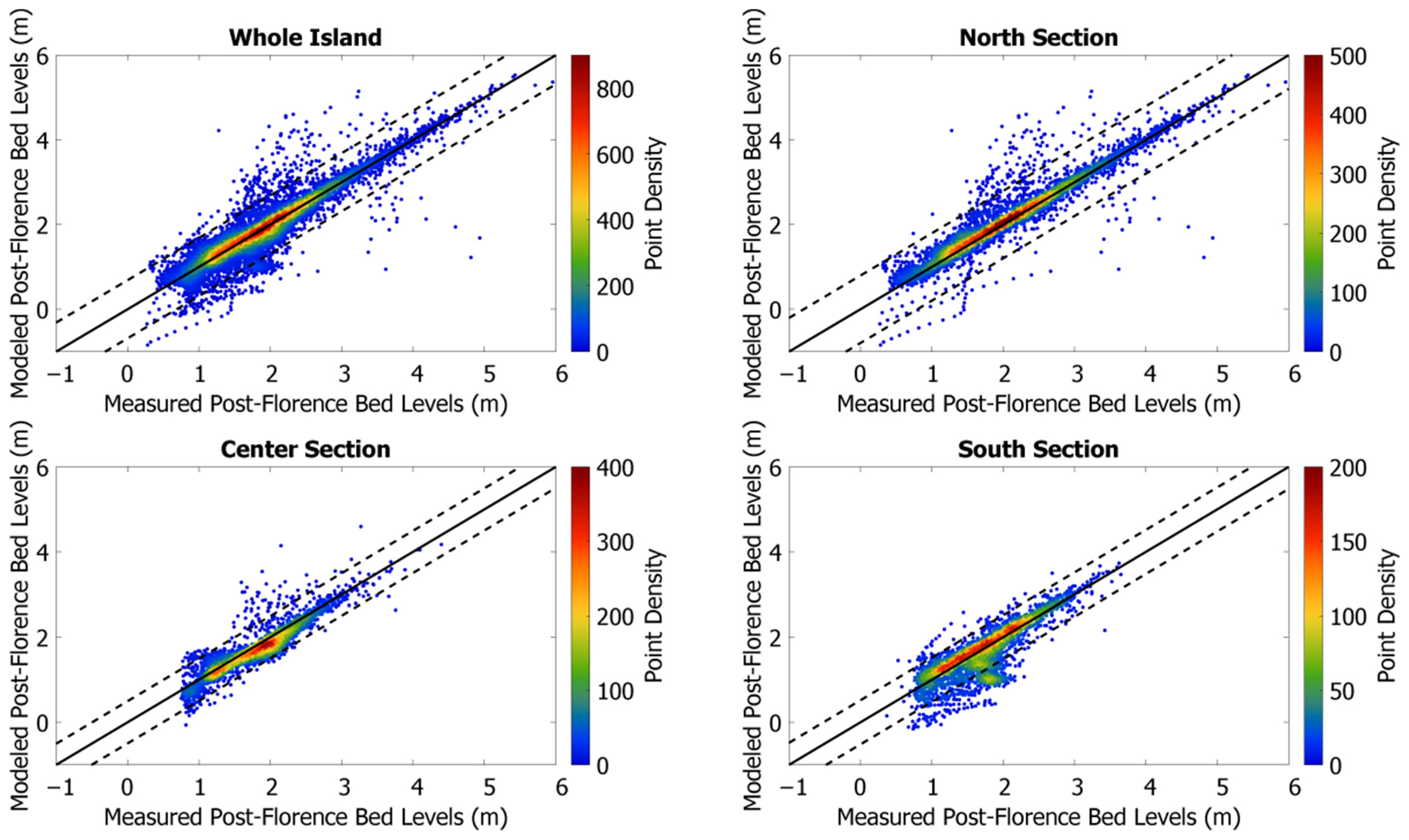
Comparisons between measured and modeled post-Florence bed level changes for the baseline simulation are shown in Figure 5. Modeled post-Florence bed levels are plotted against measured post-Florence bed levels for the entire island and for the individual section. The majority of modeled post-Florence bed levels fall within one standard deviation of the measured post-Florence bed levels for the entire island (96%) and the northern (98%), central (97%), and southern sections (87%) of the island. The model overpredicts erosion at the southern section with a cluster of points falling below measured post-storm bed levels and outside one standard deviation of measured changes.
Statistics comparing modeled and measured bed-level changes for each simulation are shown in Table 5. The default simulation (constant friction and default grain sizes) had the largest error out of the simulations completed using measured directional wave spectra (RMSE of 0.33 m for the entire island) with the model overestimating erosion in the central and southern sections (biases of −0.13 m and −0.33 m, respectively). Using measured grain sizes while holding the friction constant lowered model error for the entire island with an RMSE of 0.26 m, reducing excessive erosion at central and southern sections (biases of −0.09 m and −0.11 m, respectively). Accounting for spatially varying friction while using default grain sizes also lowered model error for the entire island (RMSE of 0.29 m) but to a lesser extent compared to using measured grain sizes. With an RMSE for the entire island of 0.78 m and biases of −0.09 m and −0.10 m for the central and southern sections, the baseline simulation (measured grain sizes and variable friction) yielded results comparable to the simulation that used measured grain sizes but constant friction over land. The JONSWAP simulation (measured grain sizes and spatially varying friction over land) had the largest model error for the entire island with an RMSE of 0.45 m and overestimated erosion at the central and southern sections with biases of −0.24 m and −0.58 m, respectively. The statistics for each simulation were comparable in the northern sections where dune erosion rather than island overwash was prominent. R2 values were the highest for the grain size simulation and the baseline simulation (0.78). The lowest R2 value computed for the entire island was from the JONSWAP simulation (0.66).
3.3. Overwash Extent and Foredune Changes
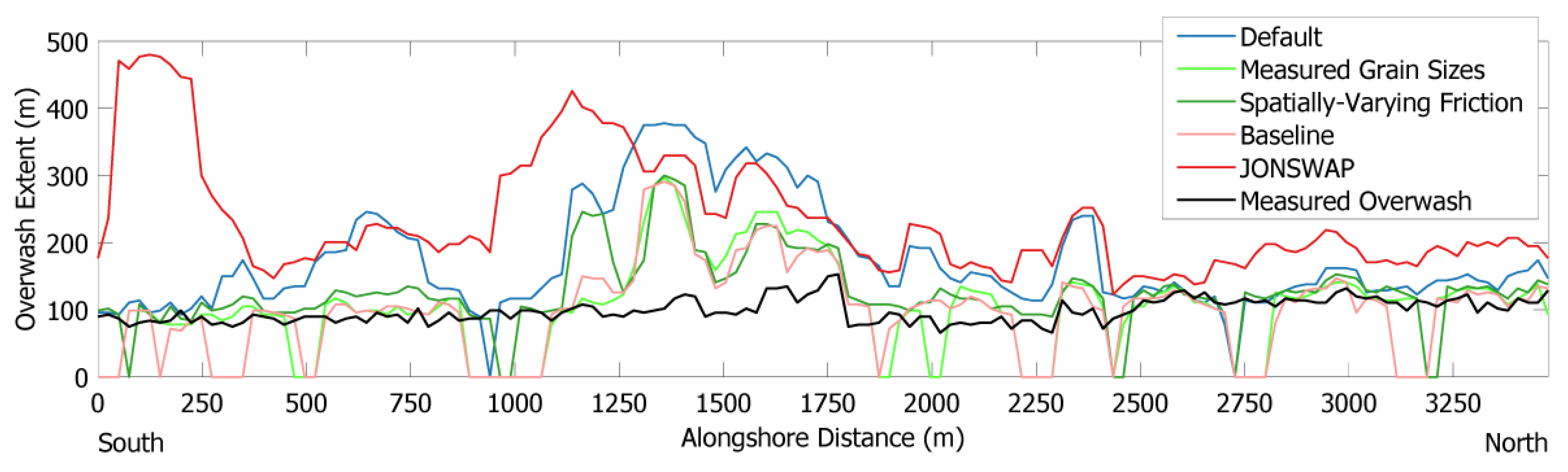
Comparisons between measured and modeled overwash extents for the different simulations are shown in Figure 6. The largest overwash extents occurred in the simulation using parameterized JONSWAP spectra. Out of the simulations using measured directional wave spectra, the default simulation had the largest overwash extents. The other three simulations yielded comparable overwash patterns and extents. Quantitative comparisons of overwash extents for this 3.5 km alongshore distance are shown in Figure 7. Overwash extents of 0 m do not indicate that no change occurred for a given cross-shore transect, only that the cross-shore transect experienced dune erosion and no overwash. The default simulation had an RMSE and bias of 107.26 m and 76.18 m, respectively, compared to measured overwash. Using measured grain sizes reduced overall overwash extents by 41% and decreased the RMSE and bias to 51.04 m and 15.00 m, respectively. The overall modeled overwash extents were reduced by 23% when incorporating spatially varying friction compared to the default simulation (RMSE and bias of 52.22 m and 30.50 m, respectively, compared to measured overwash). Incorporating both spatially varying friction and measured grain sizes (baseline simulation) reduced overwash extents by 44% resulting in the lowest RMSE (48.90 m) and model bias (10.70 m) compared to measured overwash. Forcing the model hydrodynamics with bulk spectra (JONSAWP simulation), instead of measured directional wave spectra, increased overwash extents by 52% compared to the default simulation (RMSE and bias of 161.98 m and 135.25 m, respectively, compared to measured overwash).
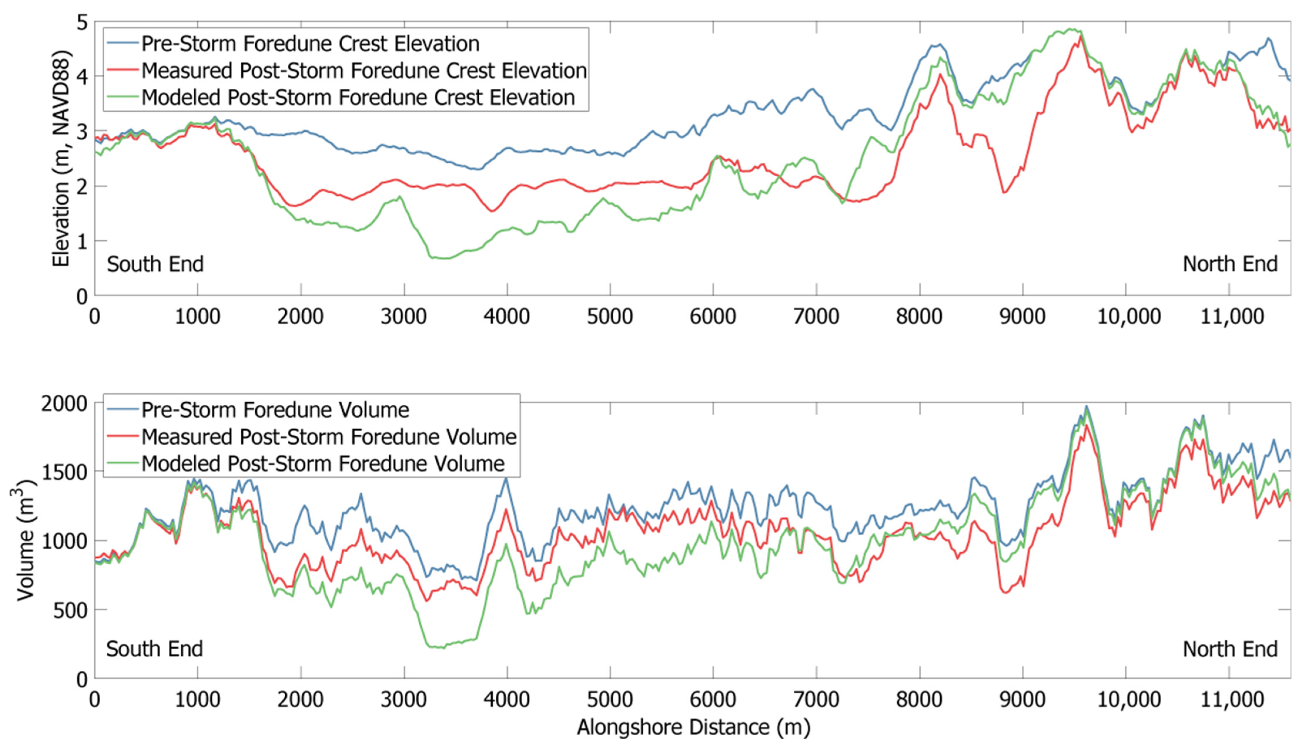
Comparisons between measured and modeled changes to foredune crest elevation and volume for the baseline simulation are shown in Figure 8. The RMSE and bias for foredune crest elevation for the entire island were 0.72 m and −0.04 m, respectively, and the RMSE and bias for foredune volume for the entire island were 202.54 m3 and −55.36 m3, respectively. The model overpredicted changes relative to foredune crest elevation and volume at the southern (RMSE and bias of 0.63 m and −0.38 m, respectively, for elevation, and RMSE and bias of 213.51 m3 and −141.10 m3, respectively, for volume) and central sections (RMSE and bias of 0.67 m and −0.19 m, respectively, for elevation, and RMSE and bias of 218.61 m3 and −149.01 m3, respectively, for volume). The model underpredicted changes to foredune crest elevation and volume in the northern section (RMSE and bias of 0.86 m and 0.48 m, respectively, for elevation, and RMSE and bias of 169.91 m3 and 134.85 m3, respectively, for volume).
4. Discussion
Despite the hydrodynamics being forced with measured directional wave spectra and observed water level conditions, XBeach overpredicted beachface water levels at the south end of Masonboro Island. One potential source of error for modeled water levels could be the use of input water levels from the Wrightsville Beach tide gauge, located north of Masonboro Island. Predicted storm surges from the ADCIRC Surge Guidance System (ASGS) indicate that a water level gradient existed along Masonboro Island where peak water levels at the north end were ~10 cm higher than peak water levels at the south end during Hurricane Florence [45]. A gradient in base water levels can be forced in XBeach; however, due to issues with unstable model hydrodynamics, a uniform tide was applied throughout the model domain for each simulation. Errors in modeled water levels also could be attributed to forcing model hydrodynamics with the ILM2 wave buoy, which is located offshore of the northern end of Masonboro Island. Spatially homogeneous wave conditions were prescribed along the offshore boundary using the buoy observations, which neglects any alongshore variations in wave energy between the northern and southern parts of the island. The ASGS indicates a similar north–south gradient in maximum significant wave heights of ~30 cm.
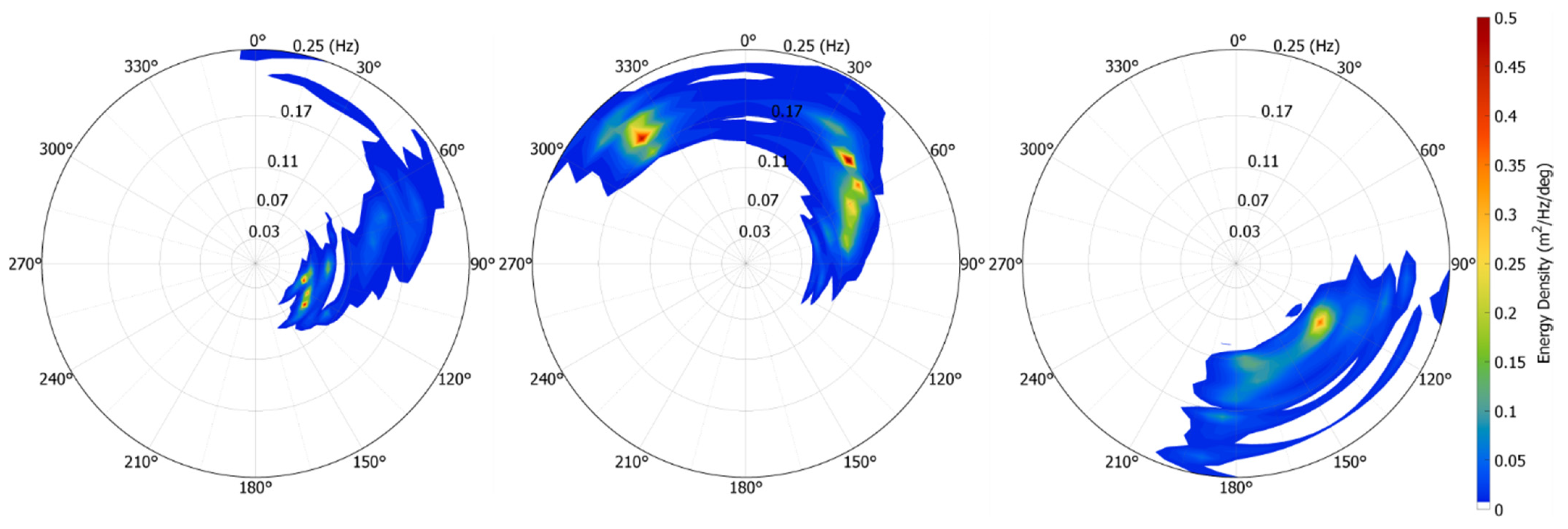
The simulation using JONSWAP spectra overpredicted the magnitude of beachface water levels and bed level changes more than the other simulations. Parameters used to calculate a JONSWAP spectra in XBeach are significant wave height, mean wave direction, and peak wave frequency. During Hurricane Florence, a bimodal directional distribution of wave energy existed where a portion of wave energy was directed offshore (Figure 9). Since JONSWAP spectra sum the wave energy across all directions and are unable to account for a bimodal directional distribution, it prescribed all of the wave energy to travel towards Masonboro Island during Hurricane Florence. Simulations using variance density spectra at the offshore boundary had lower modeled beachface water levels and reduced erosion and overwash. This result is similar to other studies (e.g., [16,26]) where higher wave heights increased model error and yielded more intense overwash and highlighted the importance of using measured or modeled full wave spectra to force the model. The other simulations showed that changes to grain size and friction did not influence modeled beachface water levels. Comparisons between modeled and measured beachface water levels assisted in assessing the model’s hydrodynamics and demonstrated that the XBeach model is capable of reproducing the timing and general magnitude of beachface water levels recorded during Hurricane Florence. However, alongshore inconsistencies exist, and additional data during storm events are needed.
Many studies have found that the use of spatially varying friction is crucial for improving model skill (e.g., [18,21,23]). In our study, however, using measured grain sizes over default grain sizes substantially improved agreements between measured and modeled changes and played a large role in reducing modeled overwash extents. This finding agrees with Matias et al. [26], who observed that finer grain sizes resulted in increased overwash likely due to reduced infiltration. It is also possible that increased critical shear stress and settling velocity from larger grain sizes limited overwash and erosion. While Matias et al. [26] used the nonhydrostatic version of XBeach, our study showed that at the barrier island scale, the ‘surfbeat’ option is capable of reproducing overwash deposits and is similarly sensitive to grain size inputs. In this study, uniform D50 and D90 values over Masonboro Island were applied, but spatial variations in grain size were observed (e.g., finer grain sizes were recorded at the north end and coarser grain sizes were recorded at the south end). Applying variable grain sizes to the model could further reduce error.
The use of spatially varying friction coefficients had less of an impact on modeled overwash extents and agreement between modeled and measured bed level changes, but they still played an important role in improving model outputs. Sentinel-2 satellite imagery offered a quick method to incorporate high resolution and up-to-date pre-storm land cover on Masonboro Island. Extreme storms such as Hurricane Florence can quickly alter existing barrier island vegetation (Figure 10), but many land cover databases used to derive friction coefficients (e.g., C-CAP or the National Land Cover Database) have temporal resolutions that are too low to capture these changes. Incorporating the effects of spatially varying vegetation allows the model to calculate more realistic flow velocities during overwash events. Model results could be improved by using a dynamic roughness model (e.g., [21,23]). Such an approach could account for changes to bed roughness during a storm where vegetation may be eroded or covered by sediment. In this study, Chezy coefficients were computed by assuming a 1 m flood depth over land, but flood depth varies temporally and spatially throughout real-world events and storm simulations. Future work could involve testing the sensitivity of Chezy coefficients to changes in flood depths and identify more realistic flood depths during the storm.
5. Conclusions
In this study, a 2D XBeach model was developed to simulate the impacts of 2018 Hurricane Florence on Masonboro Island, NC. Model sensitivity was examined with respect to different offshore spectral wave forcings, changes to grain size, and the use of spatially varying versus constant Chezy coefficients over land. Prior to the storm, cross-shore transects of water level sensors were placed at the north and south sections of the island, allowing for comparisons between measured and modeled beachface water levels during the storm. When the offshore hydrodynamics were forced using parameterized JONSWAP spectra, the model overpredicted beachface water levels, bed elevation changes, and overwash extents. Using variance density spectra to force the model’s hydrodynamics improved agreements between measured and modeled beachface water levels, bed elevation changes, and overwash extents. The use of measured or modeled full wave spectra to force models for coastal change during extreme storms is important for improving model skill and inform decision support.
Average pre-storm D50 and D90 grain sizes from the island were used to initialize the model. Measured grain sizes reduced modeled overwash extent compared to the default simulation and improved modeled bed level changes by increasing agreement between the model and observations. Changes across Wentworth grain size classes would be expected to influence the modeled elevation changes, and these simulations show that changes of ~100 microns in D50 have direct impacts on the ability to accurately predict overwash. Locations of the island that experienced dune erosion with water levels constrained to the beachface were less impacted. When possible, it is recommended that measured grain sizes should be used in place of default grain sizes for future studies using XBeach.
This study applied a technique for using pre-storm satellite imagery to calculate spatially varying friction coefficients. A land cover classification computed using pre-storm high resolution Sentinel-2 satellite imagery was used to calculate spatially varying Chezy coefficients over land. Applying high resolution spatially varying Chezy coefficients reduced modeled overwash extents, improving comparisons between measured and modeled bed level elevations. The baseline simulation that used measured grain sizes, spatially varying Chezy coefficients, and variance density spectra produced the best statistical comparisons between measured and modeled bed level elevations and resulted in the largest reduction in modeled overwash extent improving comparisons between measured and modeled overwash extents. While spatially varying friction coefficients improved model skill similar to previous studies, these results indicate that using measured grain size can be as important in accurately reproducing storm-driven morphological changes on barrier islands. The sediment characteristics on barrier islands and the time-varying wave spectra should be considered when assessing potential impacts from future storm events and scenarios.
Author Contributions
Conceptualization, J.N.B. and J.W.L.; methodology, J.N.B. and J.W.L.; software, J.N.B. and J.W.L.; validation, J.N.B.; formal analysis, J.N.B.; investigation, J.N.B., J.W.L., A.D.H., L.A.L. and E.G.; resources, J.W.L. and L.A.L.; data curation, J.N.B., J.W.L., A.D.H., E.G.; writing—original draft preparation, J.N.B. and J.W.L.; writing—review and editing, J.N.B., J.W.L., A.D.H., L.A.L. and E.G.; visualization, J.N.B.; supervision, J.W.L.; project administration, J.W.L.; funding acquisition, J.W.L., A.D.H., L.A.L. and E.G. All authors have read and agreed to the published version of the manuscript.
Funding
This research was funded, in part, by the US Coastal Research Program (USCRP) as administered by the US Army Corps of Engineers® (USACE), Department of Defense and through NSF Award # 1901894. The content of the information provided in this publication does not necessarily reflect the position or the policy of the government, and no official endorsement should be inferred. The authors’ acknowledge the USACE and USCRP’s support of their effort to strengthen coastal academic programs and address coastal community needs in the United States.
Data Availability Statement
Wave data from the offshore ILM2 Wave Buoy were obtained from https://cormp.org/ (accessed on 6 April 2021). The continuously updated digital elevation models were obtained using the data access viewer from https://coast.noaa.gov/digitalcoast/ (accessed on 13 October 2020. Drone derived elevation data are available from Long et al. [39]. The numerical model, XBeach, was downloaded from https://oss.deltares.nl/web/xbeach/home (accessed on 24 March 2020).
Acknowledgments
We would like to thank CORMP for providing open access wave data and assisting with boat transportation. The North Carolina National Estuarine Research Reserve (NERR) provided transportation, access, and permission to conduct this study on Masonboro Island. Dave Wells from the University of North Carolina, Wilmington Center for Marine Science, conducted pre- and post-storm drone flights.
Conflicts of Interest
The authors declare no conflict of interest. The funders had no role in the design of the study; in the collection, analyses, or interpretation of data; in the writing of the manuscript or in the decision to publish the results.
References
- Elliff, C.I.; Kikuchi, R.K.P. The ecosystem service approach and its application as a tool for integrated coastal management. Nat. Conserv. 2015, 13, 105–111. [Google Scholar] [CrossRef] [Green Version]
- Moffat & Nichol. North Carolina Beach and Inlet Management Plan Update; Moffat & Nichol: Long Beach, CA, USA, 2016; p. 319. [Google Scholar]
- Stive, M.J.F.; Aarninkhof, S.G.J.; Hamm, L.; Hanson, H.; Larson, M.; Wijnberg, K.M.; Nicholls, R.J.; Capobianco, M. Variability of shore and shoreline evolution. Coast. Eng. 2002, 47, 211–235. [Google Scholar] [CrossRef]
- Stutz, M.L.; Pilkey, O.H. The relative influence of humans on barrier islands: Humans versus geomorphology. In Humans as Geologic Agents; Ehlen, J., Haneberg, W.C., Larson, R.A., Eds.; Geological Society of America Inc.: Boulder, CO, USA, 2005; Volume 16, pp. 137–147. [Google Scholar] [CrossRef]
- Stutz, M.L.; Pilkey, O.H. Open-ocean barrier islands: Global influence of climatic, oceanographic, and depositional Settings. J. Coast. Res. 2011, 27, 207–222. [Google Scholar] [CrossRef]
- Kildow, J.T.; Colgan, C.S.; Johnson, P.; Scorse, J.D.; Farnum, M.G. State of the U.S. Ocean and Coastal Economies—2016 Update; Middlebury Institute of International Studies at Monterey: Monterey, CA, USA, 2016; p. 31. [Google Scholar]
- Leatherman, S.P. Barrier dune systems: A reassessment. Sediment. Geol. 1979, 24, 1–16. [Google Scholar] [CrossRef]
- Sallenger, A.H. Storm impact scale for barrier islands. J. Coast. Res. 2000, 16, 890–895. [Google Scholar]
- Mickey, R.C.; Dalyander, P.S.; McCall, R.; Passeri, D.L. Sensitivity of storm response to antecedent topography in the XBeach model. J. Mar. Sci. Eng. 2020, 8, 829. [Google Scholar] [CrossRef]
- Lorenzo-Trueba, J.; Ashton, A.D. Rollover, drowning, and discontinuous retreat: Distinct modes of barrier response to sea-level rise arising from a simple morphodynamic model. J. Geophys. Res.-Earth Surf. 2014, 119, 779–801. [Google Scholar] [CrossRef] [Green Version]
- Passeri, D.L.; Dalyander, P.S.; Long, J.W.; Mickey, R.C.; Jenkins, R.L.; Thompson, D.M.; Plant, N.G.; Godsey, E.S.; Gonzalez, V.M. The roles of storminess and sea level rise in decadal barrier island evolution. Geophys. Res. Lett. 2020, 47, 1–8. [Google Scholar] [CrossRef]
- Mickey, R.; Long, J.; Dalyander, P.S.; Plant, N.; Thompson, D. A framework for modeling scenario-based barrier island storm impacts. Coast. Eng. 2018, 138, 98–112. [Google Scholar] [CrossRef]
- Stockdon, H.F.; Thompson, D.M.; Plant, N.G.; Long, J.W. Evaluation of wave runup predictions from numerical and parametric models. Coast. Eng. 2014, 92, 1–11. [Google Scholar] [CrossRef]
- Harter, C.; Figlus, J. Numerical modeling of the morphodynamic response of a low-lying barrier island beach and foredune system inundated during Hurricane Ike using XBeach and CSHORE. Coast. Eng. 2017, 120, 64–74. [Google Scholar] [CrossRef]
- Roelvink, D.; Reniers, A.; van Dongeren, A.; de Vries, J.V.; McCall, R.; Lescinski, J. Modelling storm impacts on beaches, dunes and barrier islands. Coast. Eng. 2009, 56, 1133–1152. [Google Scholar] [CrossRef]
- McCall, R.T.; de Vries, J.; Plant, N.G.; Van Dongeren, A.R.; Roelvink, J.A.; Thompson, D.M.; Reniers, A. Two-dimensional time dependent hurricane overwash and erosion modeling at Santa Rosa Island. Coast. Eng. 2010, 57, 668–683. [Google Scholar] [CrossRef]
- Sherwood, C.R.; Long, J.W.; Dickhudt, P.J.; Dalyander, P.S.; Thompson, D.M.; Plant, N.G. Inundation of a barrier island (Chandeleur Islands, Louisiana, USA) during a hurricane: Observed water-level gradients and modeled seaward sand transport. J. Geophys. Res.-Earth Surf. 2014, 119, 1498–1515. [Google Scholar] [CrossRef] [Green Version]
- Passeri, D.L.; Long, J.W.; Plant, N.G.; Bilskie, M.V.; Hagen, S.C. The influence of bed friction variability due to land cover on storm-driven barrier island morphodynamics. Coast. Eng. 2018, 132, 82–94. [Google Scholar] [CrossRef]
- de Beer, A.F.; McCall, R.T.; Long, J.W.; Tissier, M.F.S.; Reniers, A. Simulating wave runup on an intermediate-reflective beach using a wave-resolving and a wave-averaged version of XBeach. Coast. Eng. 2021, 163, 103788. [Google Scholar] [CrossRef]
- Gharagozlou, A.; Dietrich, J.C.; Karanci, A.; Luettich, R.A.; Overton, M.F. Storm-driven erosion and inundation of barrier islands from dune-to region-scales. Coast. Eng. 2020, 158, 103674. [Google Scholar] [CrossRef]
- Johnson, C.L.; Chen, Q.; Ozdemir, C.E.; Xu, K.H.; McCall, R.; Nederhoff, K. Morphodynamic modeling of a low-lying barrier subject to hurricane forcing: The role of backbarrier wetlands. Coast. Eng. 2021, 167, 103886. [Google Scholar] [CrossRef]
- de Vet, P.L.M. Modelling Sediment Transport and Morphology during Overwash and Breaching Events. Master’s Thesis, Delft University of Technology, Delft, The Netherlands, 2014. [Google Scholar]
- van der Lugt, M.A.; Quataert, E.; van Dongeren, A.; van Ormondt, M.; Sherwood, C.R. Morphodynamic modeling of the response of two barrier islands to Atlantic hurricane forcing. Estuar. Coast. Shelf Sci. 2019, 229, 106404. [Google Scholar] [CrossRef]
- Drusch, M.; Del Bello, U.; Carlier, S.; Colin, O.; Fernandez, V.; Gascon, F.; Hoersch, B.; Isola, C.; Laberinti, P.; Martimort, P.; et al. Sentinel-2: ESA’s optical high-resolution mission for GMES operational services. Remote Sens. Environ. 2012, 120, 25–36. [Google Scholar] [CrossRef]
- Koktas, M. The Effect of Variable Grain Size Distribution on Beach’s Morphological Response. Master’s Thesis, Delft University of Technology, Delft, The Netherlands, 2017. [Google Scholar]
- Matias, A.; Carrasco, M.R.; Loureiro, C.; Masselink, G.; Andriolo, U.; McCall, R.; Ferreira, O.; Plomaritis, T.A.; Pacheco, A.; Guerreiro, M. Field measurements and hydrodynamic modelling to evaluate the importance of factors controlling overwash. Coast. Eng. 2019, 152, 103523. [Google Scholar] [CrossRef] [Green Version]
- North Carolina National Estuarine Research Reserve. Draft Management Plan 2020–2025; North Carolina National Estuarine Research Reserve: Apex, NC, USA, 2019.
- Fear, J. A Comprehensive Site Profile for the North Carolina National Estuarine Research Reserve; North Carolina National Estuarine Research Reserve: Apex, NC, USA, 2008.
- Hosier, P.E.; Cleary, W.J. Cyclic geomorphic patterns of washover on a barrier island in southeastern North Carolina. Environ. Geol. 1977, 2, 23–31. [Google Scholar] [CrossRef]
- North Carolina Coastal Resources Commission Science Panel. North Carolina Sea Level Rise Assessment Report: 2015 Update to the 2010 Report and 2012 Addendum; North Carolina Coastal Resources Commission Science Panel: Raleigh, NC, USA, 2015.
- National Hurricane Center 2018 Atlantic Hurricane Season. Available online: https://www.nhc.noaa.gov/data/tcr/ (accessed on 15 April 2021).
- Stewart, S.R.; Berg, R. National Hurricane Center Tropical Cyclone Report Hurricane Florence (Al062018); National Hurricane Center: Miami, FL, USA, 2019; p. 98.
- Holman, R.A.; Sallenger, A.H. Setup and swash on a natural beach. J. Geophys. Res. Ocean. 1985, 90, 945–953. [Google Scholar] [CrossRef]
- Ruggiero, P.; Komar, P.D.; McDougal, W.G.; Marra, J.J.; Beach, R.A. Wave runup, extreme water levels and the erosion of properties backing beaches. J. Coast. Res. 2001, 17, 407–419. [Google Scholar]
- Stelling, G.S.; Duinmeijer, S.P.A. A staggered conservative scheme for every Froude number in rapidly varied shallow water flows. Int. J. Numer. Methods Fluids 2003, 43, 1329–1354. [Google Scholar] [CrossRef]
- Cooperative Institute for Research in Environmental Sciences (CIRES). Continuously Updated Digital Elevation Model (CUDEM)—1/3 Arc-Second Resolution Bathymetric-Topographic Tiles; NOAA National Centers for Environmental Information: Boulder, CO, USA, 2014. [CrossRef]
- Cooperative Institute for Research in Environmental Sciences (CIRES). Continuously Updated Digital Elevation Model (CUDEM)—1/9 Arc-Second Resolution Bathymetric-Topographic Tiles; NOAA National Centers for Environmental Information: Boulder, CO, USA, 2014. [CrossRef]
- Amante, C.J.; Caringnan, K.S.; Love, M.; Sutherland, M. Digital Elevation Models of Southeast Atlantic Coast: Procedures, Data Sources, and Analysis; Cooperative Institute for Research in Environmental Sciences (CIRES), University of Colorado: Boulder, CO, USA, 2019; p. 6. [Google Scholar]
- Long, J.; Hawkes, A.; Ghoneim, E.; Leonard, L.; Eulie, D.; Wells, D. Pre- and Post-Storm Digital Surface Models of Masonboro Island Derived from Drone Imagery. In RAPID: Response of Hurricane Florence on Masonboro Island; DesignSafe-CI: Seattle, WA, USA, 2021. [Google Scholar] [CrossRef]
- Hasselmann, K.; Barnett, T.P.; Bouws, E.; Carlson, H.; Cartwright, D.E.; Enke, K.; Ewing, J.A.; Gienapp, H.; Hasselmann, D.E.; Kruseman, P.; et al. Measurements of Wind-Wave Growth and Swell Decay during the Joint North Sea Wave Project (JONSWAP). Ergnzungsheft zur Deutschen Hydrogr. Z. Reihe A 1973, 12, 1–95. [Google Scholar]
- Lygre, A.; Krogstad, H.E. Maximum-entropy estimation of the directional distribution in ocean wave spectra. J. Phys. Oceanogr. 1986, 16, 2052–2060. [Google Scholar] [CrossRef] [Green Version]
- Dietrich, J.C.; Westerink, J.J.; Kennedy, A.B.; Smith, J.M.; Jensen, R.E.; Zijlema, M.; Holthuijsen, L.H.; Dawson, C.; Luettich, R.A.; Powell, M.D.; et al. Hurricane Gustav (2008) Waves and Storm Surge: Hindcast, Synoptic Analysis, and Validation in Southern Louisiana. Mon. Weather Rev. 2011, 139, 2488–2522. [Google Scholar] [CrossRef]
- Donnelly, C.; Kraus, N.; Larson, M. State of knowledge on measurement and modeling of coastal overwash. J. Coast. Res. 2006, 22, 965–991. [Google Scholar] [CrossRef]
- National Geodetic Survey. 2018 NOAA NGS Emergency Response Imagery: Hurricane Florence from 2018-09-15 to 2021-09-22. Information, NOAA National Centers for Environmental Information. Available online: https://www.fisheries.noaa.gov/inport/item/57677 (accessed on 14 June 2021).
- Coastal Emergency Risks Assessment. Available online: https://cera.coastalrisk.live (accessed on 22 May 2021).
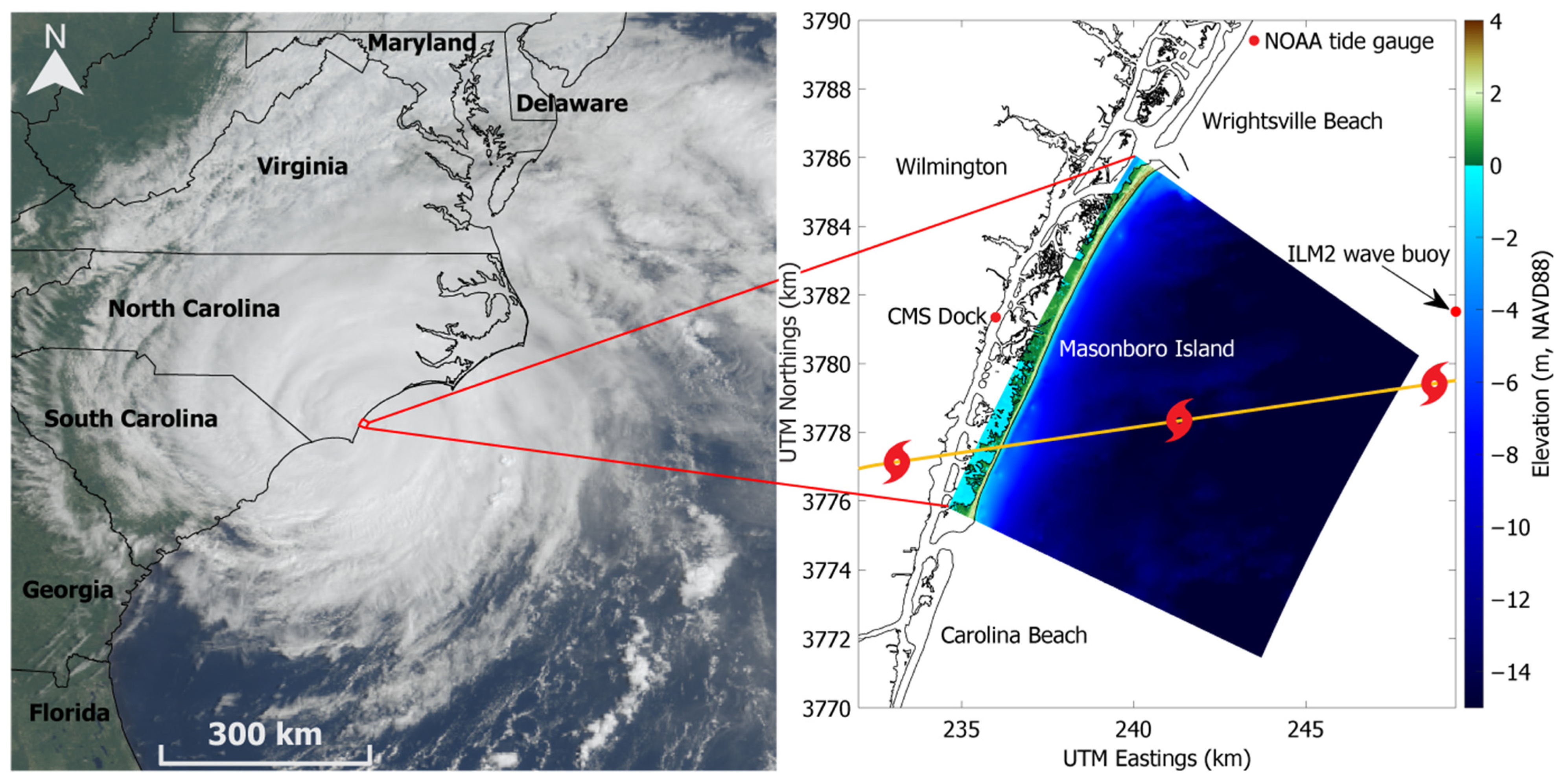
Figure 1.
GOES-16 imagery of Hurricane Florence (14 September 2018) over Wilmington, North Carolina (left), and the XBeach model domain of Masonboro Island (right) with the best track of Hurricane Florence (orange line [31]).
Figure 1.
GOES-16 imagery of Hurricane Florence (14 September 2018) over Wilmington, North Carolina (left), and the XBeach model domain of Masonboro Island (right) with the best track of Hurricane Florence (orange line [31]).

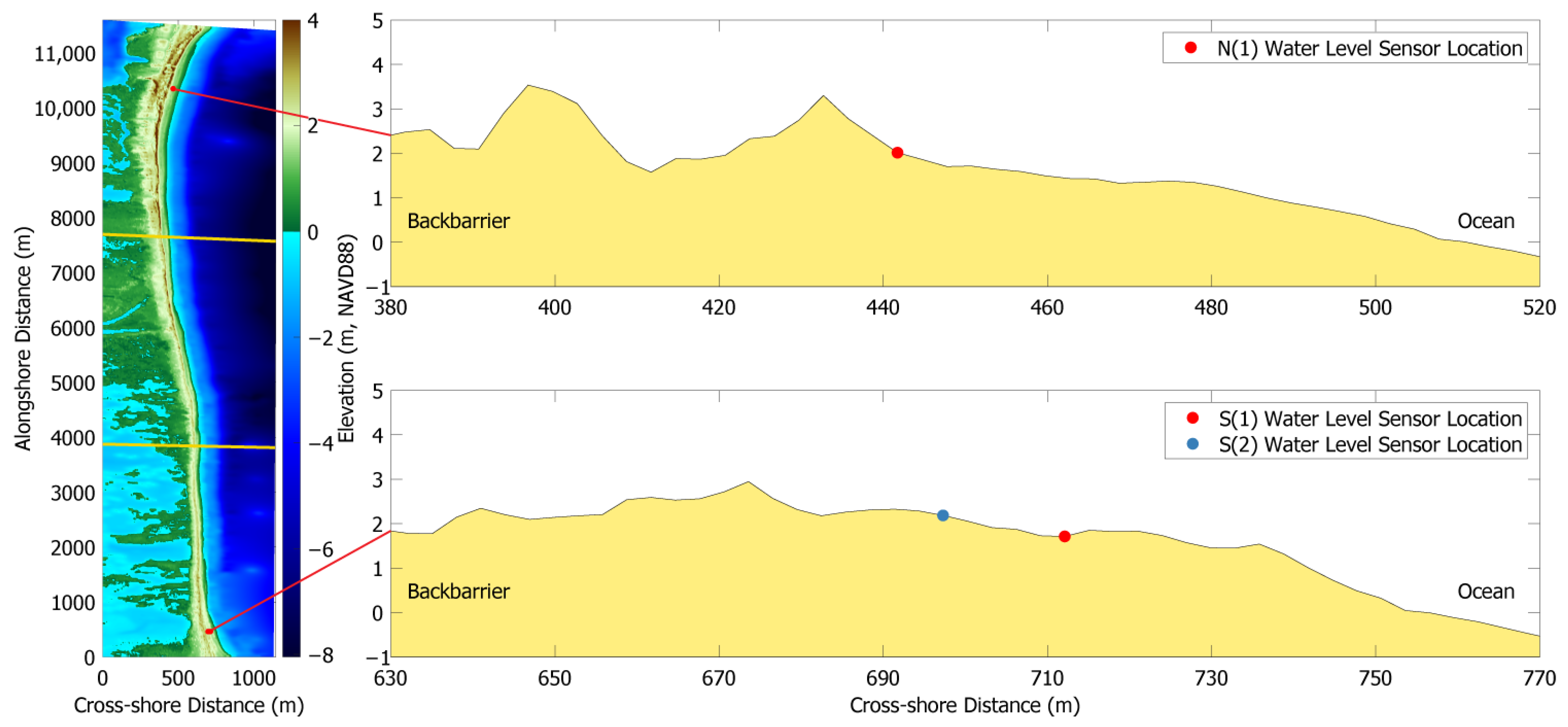
Figure 2.
Pressure sensor locations on the XBeach model domain (left) and cross-shore elevation transects (right) at the north and south sections of Masonboro Island. Additional sensors were deployed on the dune crest and behind the dune (not shown) but did not record water levels. The yellow lines on the XBeach model domain divide the northern, central, and southern sections of the island used for statistical analyses.

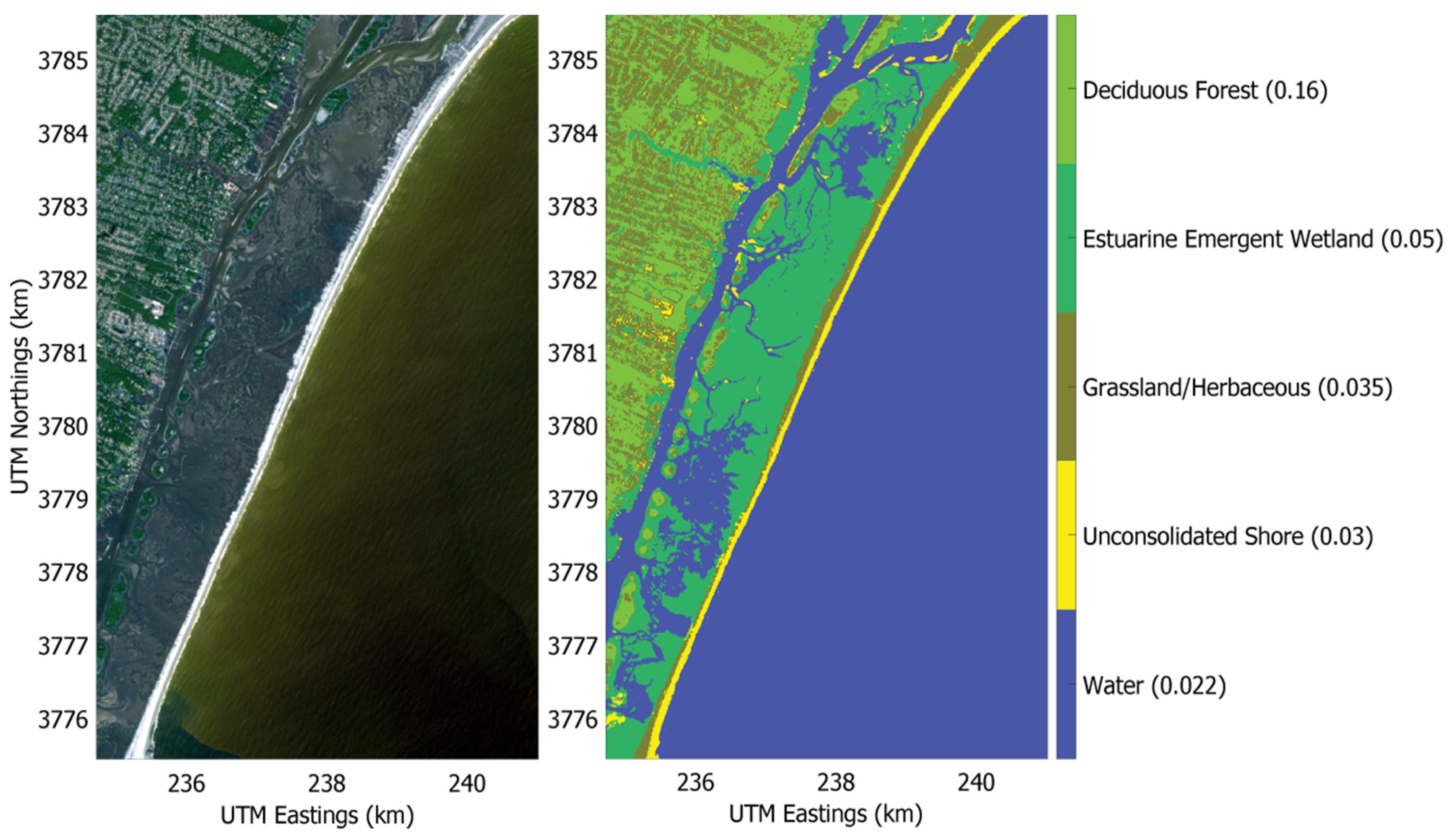
Figure 3.
Pre-storm (8 September 2018) Sentinel-2 Satellite imagery of Masonboro Island (left) and the resulting land cover classification (right) with corresponding Manning’s n coefficients (in parenthesis along color bar).
Figure 3.
Pre-storm (8 September 2018) Sentinel-2 Satellite imagery of Masonboro Island (left) and the resulting land cover classification (right) with corresponding Manning’s n coefficients (in parenthesis along color bar).

Figure 4.
Comparisons between measured and modeled beachface water levels from simulations using measured directional wave spectra (baseline simulation) and parameterized wave spectra (JONSWAP simulation). A 2 min moving average was also completed on the modeled beachface water levels.
Figure 4.
Comparisons between measured and modeled beachface water levels from simulations using measured directional wave spectra (baseline simulation) and parameterized wave spectra (JONSWAP simulation). A 2 min moving average was also completed on the modeled beachface water levels.

Figure 5.
Density scatter plots comparing measured and modeled post-Florence bed levels for the different sections of Masonboro Island from the baseline simulation. The solid black line through the origin shows a 1:1 relationship between measured and modeled elevations; the dashed black lines show one standard deviation for the measured data from the 1:1 line.

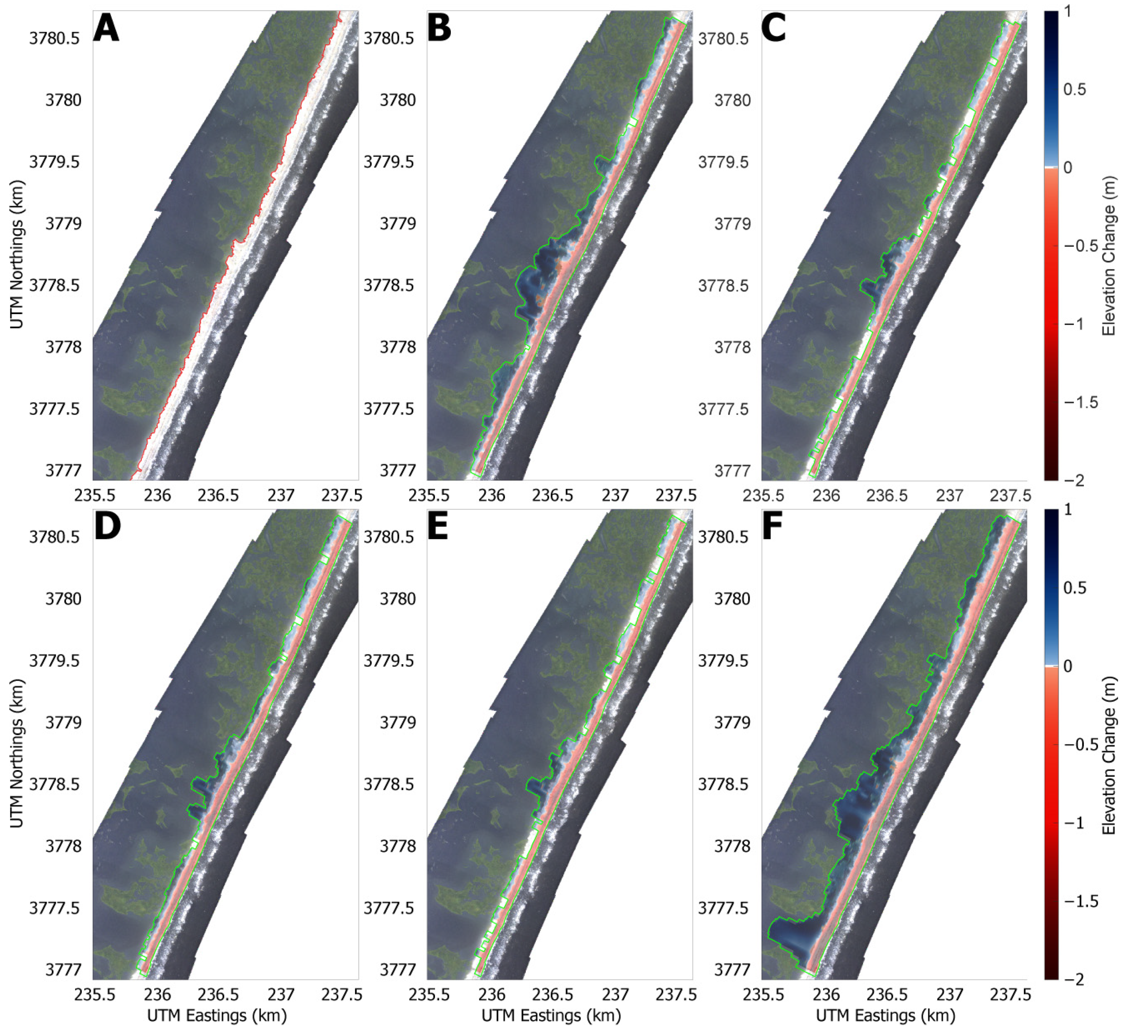
Figure 6.
NGS post-Florence imagery (A) and outlined overwash deposits for the default simulation (B), grain size simulation (C), spatially varying friction simulation (D), baseline simulation, (E) and JONSWAP simulation (F) at the southern/central section of Masonboro Island. Erosion is shown in red, and deposition is shown in blue. The green outline is the overwash polygon for each respective simulation.

Figure 7.
Comparisons between measured and modeled overwash extents for each simulation completed.

Figure 8.
Comparison between measured and modeled (baseline simulation) changes to the foredune crest (top) and foredune volume (bottom).
Figure 8.
Comparison between measured and modeled (baseline simulation) changes to the foredune crest (top) and foredune volume (bottom).

Figure 9.
Polar spectra showing the wave energy directional distribution recorded by the ILM2 wave buoy before (left, 15:00 UTC 13 September 2018), during (center, 08:30 UTC 14 September 2018), and after (right, 02:00 UTC 15 September 2018) Hurricane Florence passed over the ILM2 buoy.
Figure 9.
Polar spectra showing the wave energy directional distribution recorded by the ILM2 wave buoy before (left, 15:00 UTC 13 September 2018), during (center, 08:30 UTC 14 September 2018), and after (right, 02:00 UTC 15 September 2018) Hurricane Florence passed over the ILM2 buoy.

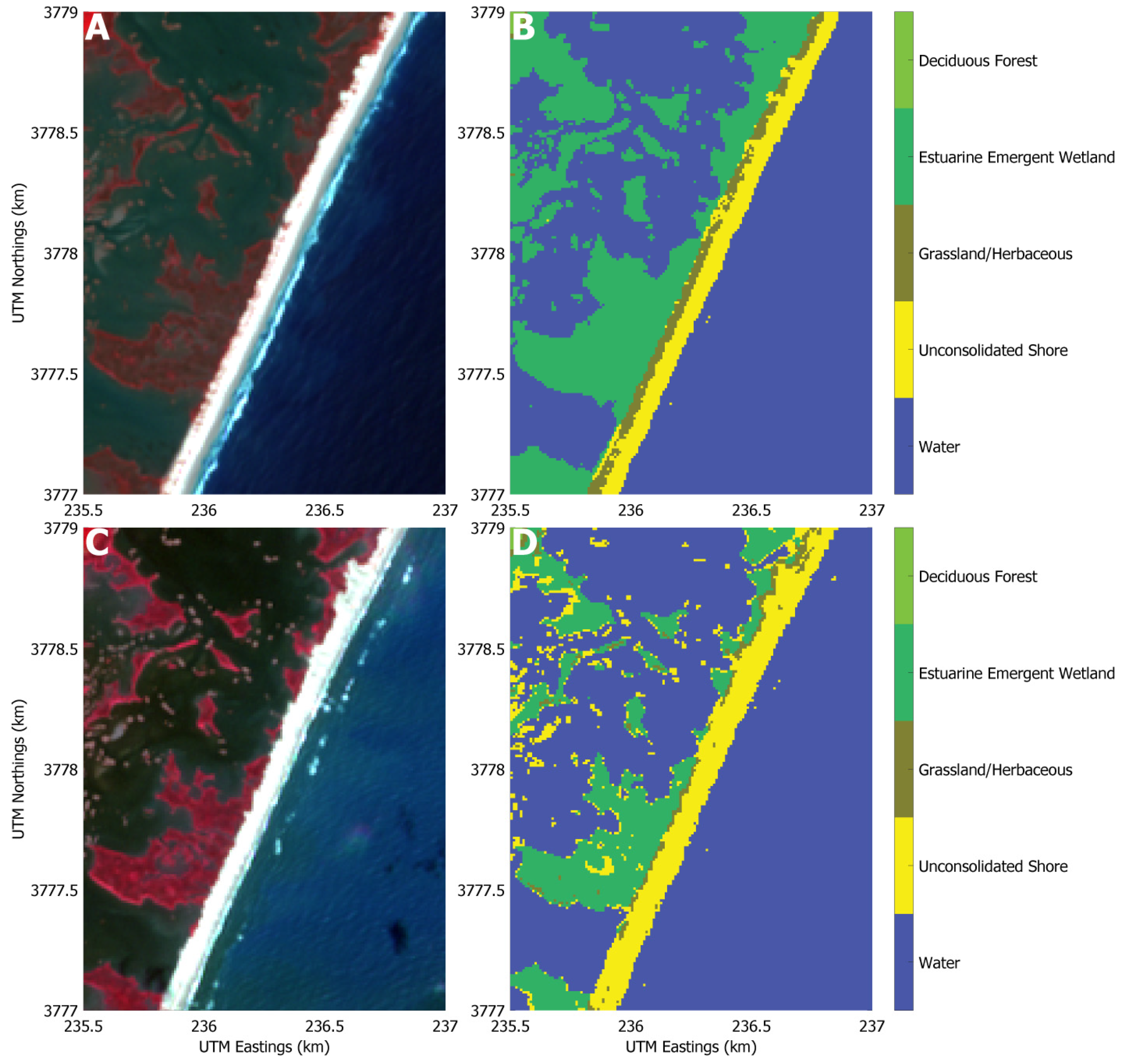
Figure 10.
Pre-Florence (8 September 2018) Sentinel-2 imagery (A) and resulting land cover classification (B) and post-Florence (18 September 2018) Sentinel-2 imagery (C) and resulting land cover classification (D) for a portion of the southern section of Masonboro Island.
Figure 10.
Pre-Florence (8 September 2018) Sentinel-2 imagery (A) and resulting land cover classification (B) and post-Florence (18 September 2018) Sentinel-2 imagery (C) and resulting land cover classification (D) for a portion of the southern section of Masonboro Island.


Table 1.
Elevation datasets used for the model domain and statistical analyses. The month and year or just the year are reported for the date collected if a specific date was unavailable for an elevation dataset.
Table 1.
Elevation datasets used for the model domain and statistical analyses. The month and year or just the year are reported for the date collected if a specific date was unavailable for an elevation dataset.
| Elevation Dataset | Spatial Resolution (m) | Vertical Accuracy (m) | Date Collected | |
|---|---|---|---|---|
| Bathymetry | ||||
| CUDEM 1/9 Arc-Second | 3 | 0.50 | 2017 | |
| CUDEM 1/3 Arc-Second | 10 | 0.50 | 2014 | |
| Topography | ||||
| 2018 USACE Post-Florence Topobathy Lidar DEM | 1 | 0.196 | October 2018 | |
| Post-Florence Drone Data | 1 | 0.086 | 10 October 2018 | |
| Pre-Florence Drone Data | 1 | 0.109 | 10 September 2018 | |
| 2017 USACE Topobathy Lidar DEM | 1 | 0.196 | 2017 |
Table 2.
Pixel counts in each training sample class.
| Class Name | Pixel Count | Area (m2) |
|---|---|---|
| Water | 14,487 | 1,448,700 |
| Bare Land | 1070 | 107,000 |
| Grassland/Herbaceous | 541 | 54,100 |
| Wetland | 617 | 61,700 |
| Forest/Trees | 681 | 68,100 |
Table 3.
Confusion matrix for the pre-Florence land cover classification and associated accuracy assessments. Bolded numbers indicate the correct number of pixels identified in each class.
Table 3.
Confusion matrix for the pre-Florence land cover classification and associated accuracy assessments. Bolded numbers indicate the correct number of pixels identified in each class.
| Land Cover Class | Water | Unconsolidated Shore | Grassland/Herbaceous | Estuarine Emergent Wetland | Deciduous Forest | Total |
|---|---|---|---|---|---|---|
| Water | 98 | 1 | 0 | 1 | 0 | 100 |
| Unconsolidated Shore | 10 | 71 | 2 | 2 | 0 | 85 |
| Grassland/Herbaceous | 0 | 1 | 24 | 0 | 2 | 27 |
| Estuarine Emergent Wetland | 21 | 1 | 3 | 67 | 0 | 92 |
| Deciduous Forest | 0 | 0 | 0 | 3 | 8 | 11 |
| Total | 129 | 74 | 29 | 73 | 10 | 315 |
| User’s Accuracy (%) | 98 | 83 | 89 | 73 | 73 | |
| Producer’s Accuracy (%) | 76 | 96 | 83 | 92 | 80 | |
| Overall Accuracy (%) | 85 | |||||
| Kappa Coefficient | 0.80 |
Table 4.
Major parameters changed for the simulations completed.
| Simulation Identifiers | Friction Type | Grain Sizes | Wave Spectra Type |
|---|---|---|---|
| Default | Constant | Default | Variance Density |
| Baseline | Spatially Varying | Measured | Variance Density |
| Grain Size | Constant | Measured | Variance Density |
| Spatially Varying Friction | Spatially Varying | Default | Variance Density |
| JONSWAP | Spatially Varying | Measured | JONSWAP |
Table 5.
Statistics comparing measured and modeled post-Florence bed levels for the different simulations.
Table 5.
Statistics comparing measured and modeled post-Florence bed levels for the different simulations.
| Section | Statistic | Constant Land, Default Grain | Constant Land, Measured Grain | Variable Land, Default Grain | Variable Land, Measured Grain | Variable Land, Measured Grain, Parameterized Spectra |
|---|---|---|---|---|---|---|
| North | RMSE (m) | 0.20 | 0.24 | 0.21 | 0.23 | 0.18 |
| Bias (m) | 0.05 | 0.07 | 0.05 | 0.07 | 0.02 | |
| R2 | 0.91 | 0.88 | 0.90 | 0.89 | 0.93 | |
| Center | RMSE (m) | 0.27 | 0.22 | 0.23 | 0.21 | 0.43 |
| Bias (m) | −0.13 | −0.09 | −0.08 | −0.09 | −0.24 | |
| R2 | 0.77 | 0.85 | 0.75 | 0.86 | 0.52 | |
| South | RMSE (m) | 0.52 | 0.34 | 0.42 | 0.34 | 0.73 |
| Bias (m) | −0.33 | −0.11 | −0.18 | −0.10 | −0.58 | |
| R2 | 0.54 | 0.61 | 0.51 | 0.59 | 0.54 | |
| Entire Island | RMSE (m) | 0.33 | 0.26 | 0.29 | 0.26 | 0.45 |
| Bias (m) | −0.14 | −0.04 | −0.07 | −0.04 | −0.27 | |
| R2 | 0.74 | 0.78 | 0.72 | 0.78 | 0.66 |
Publisher’s Note: MDPI stays neutral with regard to jurisdictional claims in published maps and institutional affiliations. |
© 2021 by the authors. Licensee MDPI, Basel, Switzerland. This article is an open access article distributed under the terms and conditions of the Creative Commons Attribution (CC BY) license (https://creativecommons.org/licenses/by/4.0/).
Share and Cite
MDPI and ACS Style
Beckman, J.N.; Long, J.W.; Hawkes, A.D.; Leonard, L.A.; Ghoneim, E. Investigating Controls on Barrier Island Overwash and Evolution during Extreme Storms. Water 2021, 13, 2829. https://doi.org/10.3390/w13202829
AMA Style
Beckman JN, Long JW, Hawkes AD, Leonard LA, Ghoneim E. Investigating Controls on Barrier Island Overwash and Evolution during Extreme Storms. Water. 2021; 13(20):2829. https://doi.org/10.3390/w13202829
Chicago/Turabian StyleBeckman, Jesse N., Joseph W. Long, Andrea D. Hawkes, Lynn A. Leonard, and Eman Ghoneim. 2021. "Investigating Controls on Barrier Island Overwash and Evolution during Extreme Storms" Water 13, no. 20: 2829. https://doi.org/10.3390/w13202829
Note that from the first issue of 2016, this journal uses article numbers instead of page numbers. See further details here.