
Assessment of the Disaster Resilience of Complex Systems: The Case of the Flood Resilience of a Densely Populated City


Department of Sciences, Technologies and Society, Scuola Universitaria Superiore IUSS Pavia, 27100 Pavia, Italy
*
Author to whom correspondence should be addressed.
Water 2021, 13(20), 2830; https://doi.org/10.3390/w13202830
Submission received: 30 August 2021
/
Revised: 4 October 2021
/
Accepted: 7 October 2021
/
Published: 12 October 2021
(This article belongs to the Section Water Resources Management, Policy and Governance)
Abstract
:In the last decades, resilience became officially the worldwide cornerstone to reduce the risk of disasters and improve preparedness, response, and recovery capacities. Although the concept of resilience is now clear, it is still under debate how to model and quantify it. The aim of this work was to quantify the resilience of a complex system, such as a densely populated and urbanized area, by modelling it with a graph, the mathematical representation of the system element and connections. We showed that the graph can account for the resilience characteristics included in its definition according to the United Nations General Assembly, considering two significant aspects of this definition in particular: (1) resilience is a property of a system and not of single entities and (2) resilience is a property of the system dynamic response. We proposed to represent the exposed elements of the system and their connections (i.e., the services they exchange) with a weighted and redundant graph. By mean of it, we assessed the systemic properties, such as authority and hub values and highlighted the centrality of some elements. Furthermore, we showed that after an external perturbation, such as a hazardous event, each element can dynamically adapt, and a new graph configuration is set up, taking advantage of the redundancy of the connections and the capacity of each element to supply lost services. Finally, we proposed a quantitative metric for resilience as the actual reduction of the impacts of events at different return periods when resilient properties of the system are activated. To illustrate step by step the proposed methodology and show its practical feasibility, we applied it to a pilot study: the city of Monza, a densely populated urban environment exposed to river and pluvial floods.
Keywords:
resilience; disaster; urban; pluvial flood; river flood; graph theory; systemic risk; complex system1. Introduction
At the Third World Conference on Disaster Risk Reduction (3rd WCDRR, Sendai, 2015), states confirmed their commitment to disaster risk reduction by building societies more resilient to disasters. With this stance, resilience became officially the foundation of the disasters risk reduction components: preparedness, response, and recovery capacities. The institutional recognition of the resilience role is part of a long process with broad and deep debate in the scientific community and beyond [1].
The origin and etymology of the concept of resilience derive from the Latin word resilio or resilire, which means “to jump back” [2,3] and its evolution until today and its relevance to the context of disaster risk reduction is well represented in Alexander (2013) [4]. According to C. G. Burton (2015) [5], Timmerman in 1981 [6] was the first author to coin the term resilience in the scientific context of natural hazards and disasters, and in his work, resilience represents the measure of “the capacity of a system, or part of a system, to absorb or recover from an adverse event”. At the beginning of the 21st century, Adger (2000) [7] extended Holling’s concept of ecological resilience to human communities.
During the last thirty years, reaching an agreement on what resilience means has been one of the most intense debates in the academic and institutional spheres [8]. In parallel to these open debates, the concept of resilience has been accompanied by its constant inclusion in major international frameworks (e.g., Sendai Framework for Disaster Risk Reduction [9] and the subsequent Sustainable Development Goals). Those works have made the resilience a very popular concept and promoted different scientific frameworks, models, and metrics to measure disaster resilience at different scales—local, national, regional, and global [5,10,11,12,13,14,15,16,17]. The 4 R’S [10], DROP [13], and RIM [18] are examples of frameworks devoted to the delineation of key characteristics of resilience that facilitate the understanding of its dynamics and lay the foundations for further developments of a quantitative assessment of resilience. These works identified common attributes of resilient systems, such as combination of redundancy and efficiency, diversity and interdependency, strength and flexibility, autonomy and collaboration, and planning and adaptability [11,19,20,21].
The resilience debate in the disaster context has also been promoted by international organizations that developed alternative frameworks, namely, the City Resilience Framework by Arup, the Rockefeller Foundation [22], the Disaster Resilience Scorecard by UNISDR [23], and the World Council on City Data series ISO 37120 (WCCD 2014) [24]. The purpose of the City Resilience Index is to provide cities with a tool allowing them to identify critical areas of weakness, and actions and programs to improve the city’s resilience in four dimensions: health and wellbeing; economy and society; infrastructure and environment; and leadership and strategy. The Disaster Resilience Scorecard provides a set of assessments for a multi-stakeholder engagement that allows local governments to monitor and review progress and challenges in the implementation of the Sendai Framework for Disaster Risk Reduction: 2015–2030. Finally, the ISO 37120 defines a comprehensive set of 100 indicators that enables any city, of any size, to measure and compare its social, economic, and environmental performance in relation to other cities from around the world.
The concept of resilience has gone through a long evolution over time and different scientific and professional fields, and it has encountered different definitions and frameworks that have either evolved or, in some cases, even differentiated [4]. Zampieri (2021) [25] shows two resilience perspectives to define resilience, the ecological and the engineering, but does not directly provide a practical way to measure it [26,27]. The states’ joint commitment following the 3rd WCDRR required a univocal agreement on the definition of resilience. A univocal agreement on the definition is the first step to have unambiguous method to quantify resilience that at this stage does not exist [28,29]. To this end, the United Nations General Assembly [30] in 2017 established the open-ended intergovernmental expert working group on indicators and terminology relating to disaster risk reduction, which has defined resilience as:
“the ability of a system, community or society exposed to hazards to resist, absorb, accommodate, adapt to, transform and recover from the effects of a hazard in a timely and efficient manner, including through the preservation and restoration of its essential basic structures and functions through risk management”.[31]
In this work, we adopt this definition because it integrates two significant aspects, which are fundamental requirements for any methodology aiming at assessing the resilience and upon which hinges the development of the proposed methodological framework:
- (1)
- Resilience is a property of a system and not of single entities, which implies the adoption of a systemic approach;
- (2)
- Resilience is a property of the system’s dynamic response, which implies the definition of rules on how the system can adapt to, transform, and recover from the aftermath of a hazardous event.
Metzger, Robert, and Área (2013) [32] pointed out that when the concept of resilience is applied to an entire system and not to a specific element or object, resilience is conceptually assimilated to a complex system. The complexity, which emerges at the system level, is derived from the non-linearity and multiplicity of the dynamic interactions between many elements of different types that make up the system [33]. The stress induced by perturbations to the complex system can generate three types of response: (1) the system could absorb the stress and come back to the original equilibrium, (2) it could adapt and evolve to a new equilibrium configuration, (3) fundamental and irreversible changes cause the system to lose its structure [4,34,35].
The debate on what makes a complex system resilient, the variables to measure and to monitor it and, therefore, to improve it, has not yet been clearly defined both at a theoretical and applicative level [12]. In this open discussion, Arosio et al. (2020) [36] proposed a paradigm shift from a reductionist to a holistic approach to assess natural hazard risk supported by the construction of a graph. The graph is constructed by identifying the two main objects, i.e., nodes and links, and their characteristics. Each node can provide or receive service to or from others (links). Once the terms of the connections between the different node categories are defined, it is crucial to establish the rules to determine if two nodes belonging to different categories should be linked. Once the nodes and the rules to link the various services are laid out, the graph is built, and the relevant graph attributes can be computed and assigned to its nodes or links. This proposed approach allows us to describe the properties of the entire system itself and demonstrates the advantages of representing a complex system, such as an urban settlement, through a graph and using the techniques made available by the branch of mathematics called graph theory. Furthermore, Arosio et al. (2020) [37] applied the methodology to estimate the total impact using the graph representation of a system as the basis for assessing higher-order impacts and cascading effects for different return periods (T), based on the propagation of impacts along graph links.
Fekete (2019) [38] proposed a conceptual framework to show the interrelation between resilience and cascading effects in the traditional critical infrastructures (CI) risk context. He identified three critical (i.e., essential or most relevant) system features: (1) critical quantity (volume); (2) critical time factors (on-set speed, duration, temporality); (3) quality [39]. The dependency and interdependency have been thoroughly analyzed in CI [40], and Rinaldi et al. (2001) [41] proposed a comprehensive framework to identify, understand, and analyze the challenges and complexities of interdependency. These interdependencies are crucial for understanding how the impacts of natural hazards propagate across infrastructures and towards society. Zorn et al. (2020) [42] proposed a methodology to combine functionally interdependent infrastructure networks with geographic interdependencies by simulating complete asset failures across a national scale grid of spatially localized hazards, and the application in New Zealand (across energy, telecommunications, and transports infrastructures) highlighted the importance of considering infrastructures interdependencies when assessing systemic vulnerabilities and risks to enhance resilience. Roy (2020) [43] proposed an approach to identify the co-occurrence of multiple infrastructure disruptions using social media data and a method to visualize disruptions in a dynamic map. At a national level, Papillous (2020) [44] demonstrated the importance of an appropriate choice of methods in flood road exposure analysis, and it also showed a new way of flood road exposure assessment taking into account the whole system as a network. Instead, in the context of a flood in a metropolitan area, Arrighi (2021) [45] presented the risks due to systemic interdependency between the water distribution system (WSS) and the road network system.
Pant et al. (2018) [46] proposed a spatial network model to quantify flood impacts on infrastructures in terms of disrupted customer services directly and indirectly linked to flooded assets. Koks (2019) [47] presented a spatially explicit integration of critical infrastructure failure with a state-of-the-art multiregional macroeconomic modeling framework, able to capture business disruption due to flood hazard from the supply-side, as well as demand-side, disruptions. These analyses could inform flood risk management practitioners to identify and compare critical infrastructure risks on flooded and non-flooded land to prioritize flood protection investments and improve cities’ resilience.
This short literature review, even if it does not cover completely the very broad resilience sector, highlights some main issues that are still open for a more exploration in the scientific community:
- There is not yet a consolidated approach to quantitatively measure the resilience that takes into account its fundamental properties as appointed in the UNGA’s definition;
- The assessments of disaster risk and resilience are independent and incoherent, although they both refer to the same catastrophic events and have the same scope;
- Even the well-developed branch of research on infrastructure resilience does not adopt a systemic approach: the analysis is mostly focused on the efficiency of a single infrastructure typology rather than on the impact that its failure may have on society or, in general, on the whole system.
Considering this context and the discussed open issues, the aims of this work were:
- To quantify disaster resilience of a complex system by means of the graph;
- To be compliant with the resilience definition by the UNGA;
- To adapt the traditional risk assessment methodology to the concept of resilience;
- To demonstrate the feasibility of the proposed methodology with a case study;
- To discuss the limits of the methodology and to propose future developments.
2. Methodology
2.1. Theoretical Framework
In this paragraph, we present the theoretical framework of the methodology to assess the resilience of a complex system.
When a hazardous event hits a system, the elements can be either directly or indirectly impacted. The directly impacted elements experience physical damages (e.g., a building damaged by a hurricane), but they could also experience indirect consequences (e.g., business interruption), which are non-physical damages. Other elements of the system, although not directly impacted by the event, could experience non-physical damages because of the dependency on (directly or indirectly) impacted elements. Table 1 summarizes these types of impacts.
In most of the applications, the assessment of the risk considers only the first type of damages (a), physical damages at directly impacted elements. Some applications take into consideration also the second type of impact (b), the consequent non-physical damages at directly impacted elements. Very rarely, the assessment of risk adopts a system perspective and considers also the third type of impacts (c), the non-physical damages at indirectly impacted elements due to services interruption from directly impacted elements. For the sake of the system all the three types of impacts are relevant when the indirect non-physical damages are the most relevant.
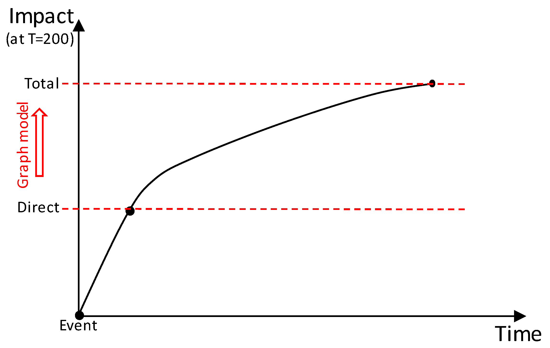
In order to consider them, one needs to (know and to) model how each element is connected to another, which, in other words, means to model the system as a whole instead of modeling single elements. The connection between exposed elements constitutes a network that, in the case of a hazard, propagates the impacts along the system (the so-called cascading effects). Being a network, the system can be mathematically represented by a graph [36]. Figure 1 conceptually shows how the impacts of a hazardous event are propagated: at first, only directly impacted elements are accounted for, then elements indirectly impacted by them, and thereafter, in sequence, all the other elements connected to those. Therefore, the total, overall, impact of the event over the system is much larger than only the direct impact. The graph model proposed by Arosio et al. [36] is designed to assess the total impact. In this paper, we present a step forward with regard to the previous model that enables the graph to take into account the capacity of the system to resile to the hazardous event. It has the same network nature of the system that, on one hand, propagates the impacts, on the other hand, supplies resources to dynamically react and “jump back” to an equilibrium state.
For an in-depth description of the model, please refer to Arosio et al. [36,37]. For the sake of clarity, we recapitulate here only the main features of the methodology that are necessary to ease the understanding of the innovations brought by the model, which are, in brief, (1) the construction of a redundant and weighted graph, (2) the definition of adaptation rules to dynamically adjust the graph configuration.
The graph consists of two types of network objects, nodes and links, and their characteristics. Formally, a graph G consists of a finite set of elements V(G) called vertices (or nodes), and a set E(G) of pairs of elements of V(G) called edges (or links) [48]. Graphs can be directed or undirected, weighted or unweighted [49].
In more practical terms, the mathematical graph G, built from a list of nodes V(G) and links E(G) can be obtained using the open source igraph package for network analysis in the R environment (http://igraph.org/r/, accessed on 11 September 2021). The full library of functions adopted here to compute the graph properties is provided by Nepusz and Csard (2018) [50].
Mathematical properties of a graph can be studied using graph theory [51,52]. These properties, such as degree, hub, and authority values, are useful metrics to analyze the graph structure (i.e., network topology and arrangement of a network) and to characterize elements from a systemic viewpoint (e.g., [53]). Arosio et al. (2020) [36] showed that graph properties can also disclose some relevant characteristics of the risk of the system to different hazards as well as vulnerability and exposure features.
The importance of a node in directed graphs, within the purpose of providers that deliver a service, is closely connected with the concept of topological centrality: the capacity of a node to influence, or be influenced by, other nodes by virtue of its connectivity. In graph theory, the influence of a node in a network can be provided by the eigenvector centrality of which the hub and authority measures are a natural generalization [54]. A node with a high hub value points to many nodes, while a node with a high authority value is linked by many different hubs. In particular, the authority represents how the system privileges the nodes, conferring them more or less importance compared with others, according to the connections established in the system (i.e., exposure). On the other hand, a hub measures the vulnerability of the system as a whole and shows the propensity of parts of the network to generate a cascading effect after hazard events.
Arosio et al. [37] modeled the propagation of the hazard impact in the system with the graph but without any possibility to absorb or adapt to the perturbation by changing its configuration. We call this graph “static” and therefore not suitable to represent the resilience of the system.
In this paper, instead, we build a different graph configuration in order to account for the resilience characteristics of a system to natural hazards, and we defined rules to allow the system to dynamically adapt to them. Doing so, we believed getting closer to the resilient behavior of complex systems as it is observed in reality. Furthermore, a graph model that embeds the resilience characteristics of the system experiences ultimately a reduced impact. Therefore, the resilience can be quantitatively assessed by the risk reduction.
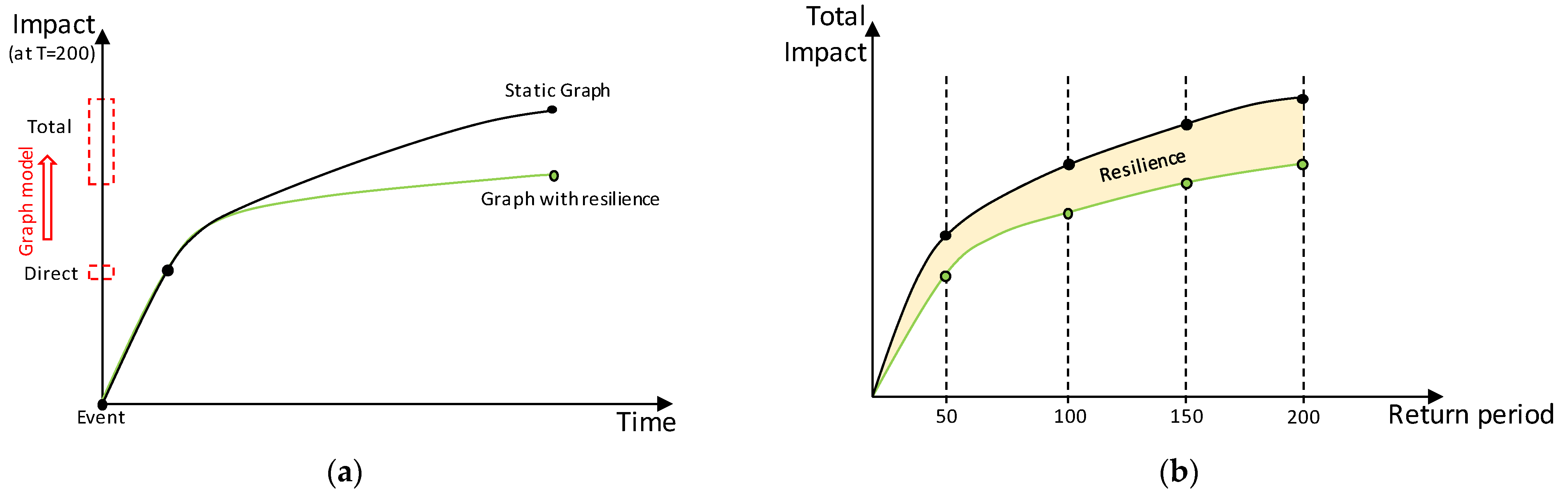
Figure 2a shows the total impact for different hazard probabilities and for two graph configurations: with and without resilient characteristics. The resilience of the system can be visualized (and computed) as the area between the two risk curves, as illustrated in Figure 2b. The methodology of this framework can be summarized in the following steps:
- Built the graph [36,37]: one without and one with resilience characteristics (as described in Section 2.2.1);
- Perturb the graphs by an external hazard (as presented in Section 2.2.2);
- Use the graph to propagate the indirect impacts (as described in Section 2.2.2);
- Built the risk curves for the two different graphs (theoretically introduced in Section 2.1 and results presented in Section 3.2);
- Estimate resilience as the area between the two curves (as described in Section 3.2).
The details of each step are presented in the following sections.
2.1.1. System Perspective: Building the Graph
The proposed methodology adopts a systemic structure which makes it possible to build and describe the entire system properties by a graph. The methodology is based on the graph’s construction by establishing the graph’s two main objects, nodes and links, and their characteristics. Depending on the specific context of the analysis, the categories (i.e., taxonomy, e.g., public office, education, leisure) of the most relevant elements (nodes) exposed to the hazard are selected. Those nodes are relevant in the systems for the function they assume in the system. Each node can provide or receive service to or from others (links). Links can be of different types according to the nature of the connection: physical, geographical, cyber, or logical [41].
Translating exposed assets and intricacies of their connections to a conceptual network requires some assumptions and simplifications according to the data at disposal regarding the exposed goods. Indeed, the different element types that constitute the features and functions of the city are represented by a number of categories that depend on the data availability of the study case. Once the terms of the connections between the different categories are defined, it is crucial to establish the rules to determine if two nodes belonging to different categories should be linked. In the real world, not all services have the same importance and the same spatial range. For instance, a local grocery store and a hospital have different roles and users. Therefore, different rules are necessary to connect two nodes according to their type, bringing in further assumptions.
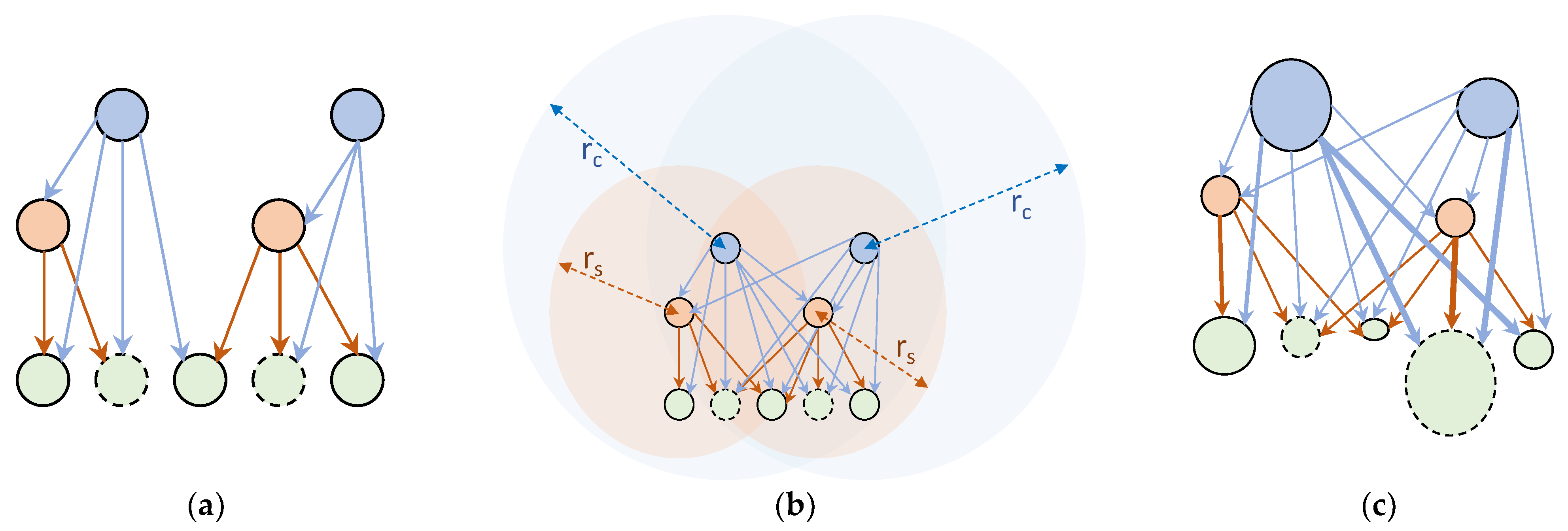
In this methodology, there are two major topological improvements with respect to previous works [36,37]: (1) redundancy and (2) weighting. First, each node does not receive the service only from the closest provider, but it has multiple, redundant providers that could provide the same service to it. Second, the methodology includes building of a weighted graph considering the number of people who use the single service. The illustrative example of Figure 3 shows these two innovative features that enable better reproduction of the complex interactions.
The set of rules proposed to create the links is based on a distance criterion that allows receivers to accept multiple providers per service, introducing redundancy into the network. Once the nodes and the rules to link the various services are laid out, the graph can be built, and relevant graph attributes can be computed and assigned to its nodes or links. The driving force behind these attributes’ computation stems from the inability to provide full information about the system we are trying to represent. In light of these limitations, four attributes, whose formulation is hereafter described, were attached to the graph elements, namely:
Length: a link attribute computed as the geodetic distance between two vertices of the link.
Ranking: a link attribute assigned based on the length attribute. For each type of link, one is assigned to the link connecting a receiver to the closest provider (i.e., the link with the lowest distance), assigning the subsequent ranking following the increasing distance.
Weight: a link attribute assigned to each link as a numerical value representing the number of users that the link serves in total. For example, a link connecting a shop to a residential building where ten people reside would have assigned a weight value of 10. A link connecting the industrial provider that replenishes the aforementioned shop would have a weight equal to the sum of the weights of all the links of which that shop is the provider. The weights underwent a log-transformation to overcome the wide range of values that this procedure would return.
Capacity: a node attribute attached only to those vertices providing a service. The provider’s capacity is meant as the maximum number of users it can serve in emergency conditions (i.e., when the city is hit by a hazardous event) and is estimated as the number of users served in ordinary conditions increased by a tolerance. Each provider’s capacity is estimated as the sum of the weights of link with rank equal to 1 increased by a certain percentage (e.g., 10%) to consider backup capacity.
2.1.2. Dynamic Response: Defining the Adaptation Rules
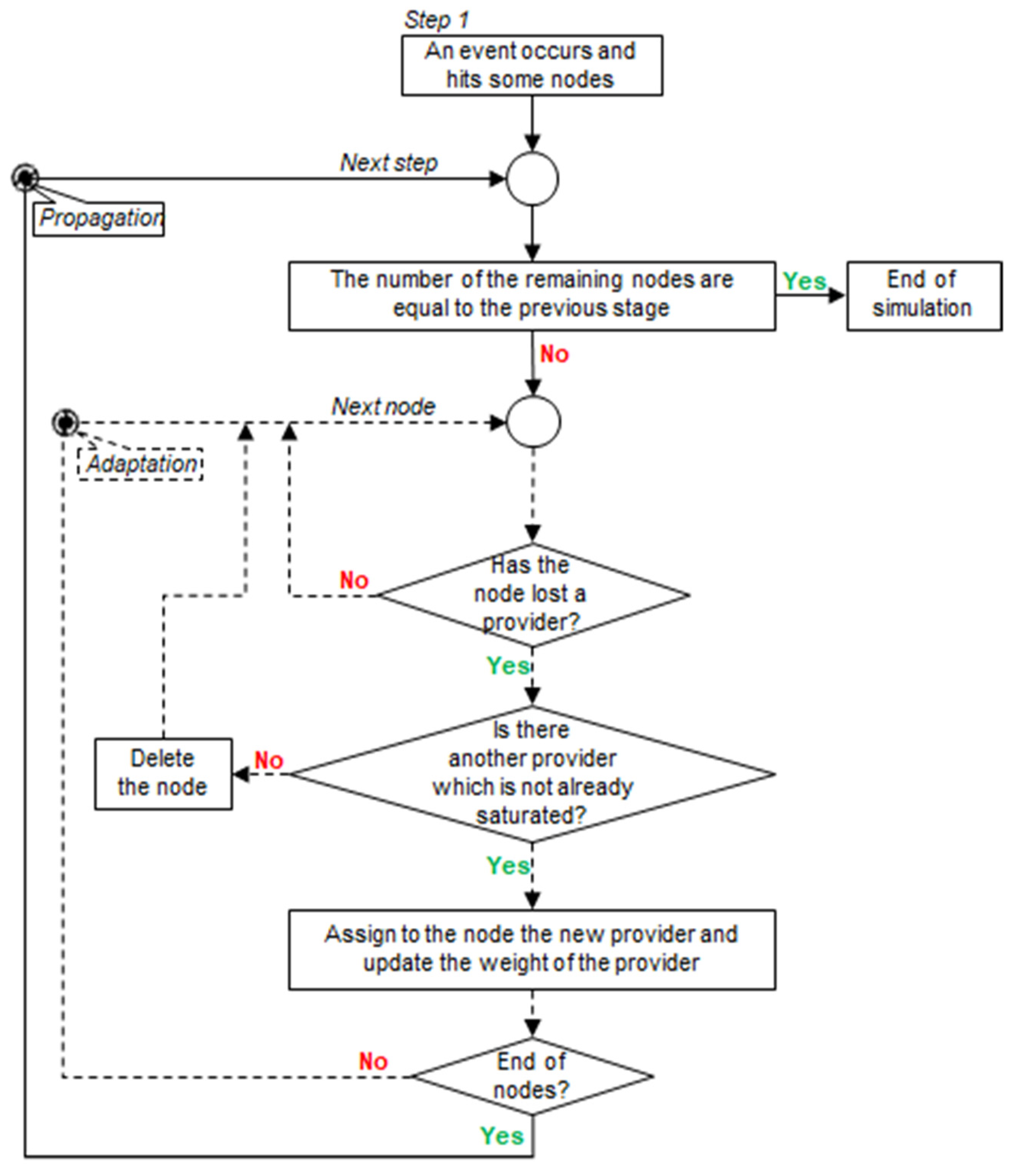
A methodology, summarized in Figure 4, to study the cascading effects of the hazard on the network elements that are not directly affected by the hazard was developed to reproduce the disruption and the adaptation capacity throughout the network.
In this work, differently from Arosio et al. [37] who consider a static structure of the exposed system, the system structure reacted dynamically to an external perturbation thanks to the network redundancy. The ability of nodes to change connections depends on the categories of nodes and the duration of the perturbation, short or long term (e.g., the road is interrupted for a couple of hours or the reconstruction of a building may require some years). In the proposed methodology, each node of the graph is connected to more than one node that provide the same type of service, and they can cope with a perturbation by changing provider: from the one in an ordinary situation to a new one in the perturbed situation.
The several steps depicted to construct the graph led to a topological graph representing an urban environment through nodes and edges. Graph theory allows us to study the property of this mathematical representation (e.g., degree, hub, authority) in the unperturbed state and after a hazard that caused a shock to the system. This process facilitates monitoring the changes in the graph’s properties ante- and post- catastrophic events, making it possible to observe how the system adapts to the shock.
2.2. Case Study: The City of Monza
The methodology proposed in this paper was applied to the case study of Monza. The city and its municipality, hosting more than 120 thousand residents, is situated in northern Italy in the Lombardy region, where it ranks third amid the most populated metropolitan areas in the region, behind Milan and Brescia.
The city is densely populated and is split in half by the Lambro River, which passes right through the city’s historical center, touching downstream Milan before flowing into the Po River. In recent years, several flooding events occurred, threatening the heterogeneous fabric of the city. Moreover, severe rainfall events highlighted the drainage system’s incapacity to cope with extreme events, thus provoking urban flooding and providing an additional hazard to the city by spatial and temporal resolution [55].
The dimension of the city allows us to study the urban system and its interdependencies at high resolution.
2.2.1. Construction of the Graph
As part of the NEWFRAME project (www.newframe.it, accessed on 11 September 2021), the Monza municipality provided us with a catalog of all the city buildings with several of their features that are reported and fully described in Table A1 in Appendix A. The characteristics of the buildings could be divided into two categories: (1) properties related to geometry (i.e., area and height) and georeferencing (i.e., addresses) of the building and (2) properties related to the destination of use and function of the edifice.
The latter features of the buildings were used to divide the network nodes into the categories reported in Table 2, along with their number and the type of nodes they serve. Each node is associated with a real physical element (e.g., a building or a major intersection), although this association is not univocal. A single building could host more than one provider or receiver of a service. Likewise, there are shops, offices on the ground floor of a building, and residential apartments on the upper floors.
Regarding the categories, the following assumptions were adopted. We deemed it essential to incorporate the transportation system into the graph, with the limitation of considering only the city’s major intersections and the bridges that pass over the Lambro River, thus slimming down the transportation system to its most relevant elements. The recovery nodes represent all those services that provide first aid, such as hospitals, firefighters, and police stations on call 24/7 and grant rescue to all the other categories. Nodes identified as industrial provide a service both to residents in the form of job opportunities and to the shops as suppliers. Lastly, there are categories of nodes that directly offer various services to the citizens or a part of them. This group comprises services such as health facilities (e.g., pharmacy, private practice), shops, public office (e.g., postal office), and leisure (e.g., cinema, arcade), which are intended for the entire population. Senior centers are intended for the elderly, the center for disability is aimed at people with some sort of handicap, and educational services are provided to the younger portion of the population. The residential typology does not provide any service but functions just as a receiver. Each building was identified as a residential node as long as at least one person was listed as resident at the address of the building. The data regarding the number of people living in each edifice were provided by the municipality. A subsequent step regarding the population entailed splitting the residents based on their age distribution (split into three groups: 0–15, 16–64, and 65+), derived from the information obtained from the parent census area provided by the National Institute of Statistics (Istat). The municipality also provided data on the proportion of the disabled people. The aforementioned population features, namely, age distribution and disability, attached to the buildings were used to refine the connections between certain categories of nodes. For example, the connection between nodes representing the center for disability and nodes representing residential building were made only where the presence of a disabled person in the building was ascertained.
Table 3 reports the list of providers alongside the type of nodes they serve and the method used to establish the connections among the three different spatial ranges used depending on the node type:
The entire city—this method was applied only to the recovery nodes. These providers are required to offer 24/7 service, and the essential nature of their assistance needs to be at the disposal of the entire city; thus, all the nodes in the city are linked to all the recovery nodes.
Parallel Bands—this method was used only for bridges that provide a service only to crossroads. The underlying idea was to separate the study area into overlapping parallel strips, where each strip is centered around and parallel to a bridge. All the crossroads falling inside such strip are linked to the bridge. Overlapping of the bands was implemented to introduce redundancy amid these two categories and simulate the possibility of choosing different paths to cross the river when the flood hits. The overlapping distance was estimated as half the longitudinal Euclidean distance between consecutive bridges. The justification for the proposed approach resides in the north-to-south distribution of the bridges that, following the river’s course, separate the city into west and east (i.e., the Lambro River flows from north to south).
Radial Area—this method was implemented for the remaining providers. The main idea was to connect all the providers to each receiver, for a given category, within a certain distance (i.e., radius). For example, a residential building is linked to all the post offices within a radius of 1 km. The distance was set as the 25th quantiles of the distance matrix for each provider–receiver couple.
As a result of the above assumptions, we represented Monza as a directed, weighted graph with 6007 nodes and almost 1.3 million links that can well represent a system’s redundancy like an urban city.
2.2.2. Impact of Hazard on the Complex System
In our study case, the system is impacted by pluvial and fluvial floods reported by Galuppini et al. [55]. The theoretical procedure presented above was used for both types of hazards and entailed evaluating, at different steps, changes in the graph’s topology and the effects that these changes caused to its properties. For the sake of clarity and due to the limited information, we considered only long-term perturbation. To simplify the computation of the hazard’s impact on the system, only a binary state was considered for each node—impacted or not. In particular, the building is impacted whenever the shape of the building intersects the extent of the flood map. In the case of the impacted, the node was removed from the graph, adopting a binary function of the vulnerability of the second order (i.e., directly impacted and therefore unavailable). Let step 0 be the graph in the unperturbed state and step 1 the graph where the nodes hit directly by the hazard are removed, a new step was computed according to the iterative procedure described in Figure 4, anytime the number of nodes in the graph decreased. For each node of the graph, it is checked whether it has lost a provider. In this case, we checked whether the node had another provider that had not yet saturated its capacity. In this case, the provider was assigned to the node. Otherwise, the node was removed from the graph. The iterative procedure continued until there were no more nodes removed at a new step.
3. Results
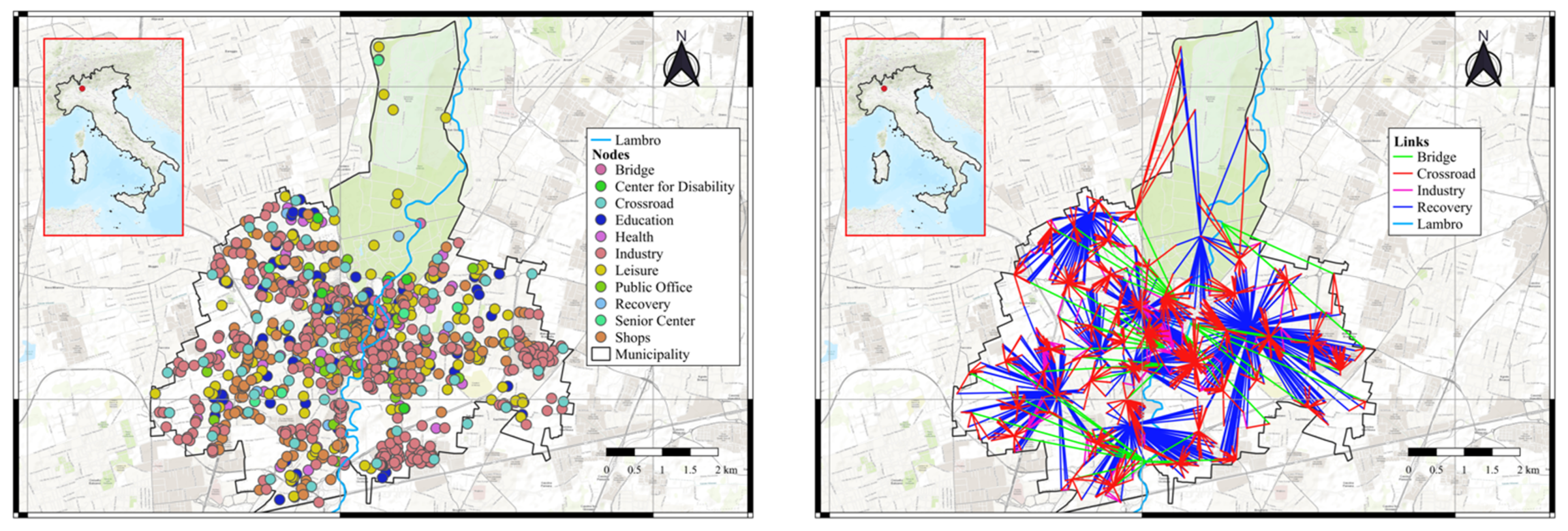
The above-described procedure was applied to the city of Monza. First we built a non-redundant unweighted graph, second a redundant and unweighted graph, and finally, the more complete redundant and weighted graph. The map in Figure 5 shows the nodes and links that form the graph. For better readability, we only report the non-redundant graph, and the resident nodes are not plotted. The color of the links depends on the typologies of the connections. The city center has a higher density of nodes and services. On the contrary, the suburban areas have more scattered services.
In the following paragraphs, the topological properties between the three different configurations explored on the Monza graph are compared; in particular, the effects of considering a weighted graph and the services redundancy are emphasized (Section 3.1). After the properties analysis, Section 3.2 presents the resilience estimation after perturbations considering only the weighted graphs: with and without redundancy.
3.1. Effect of Redundancy and Weight on Graph Properties
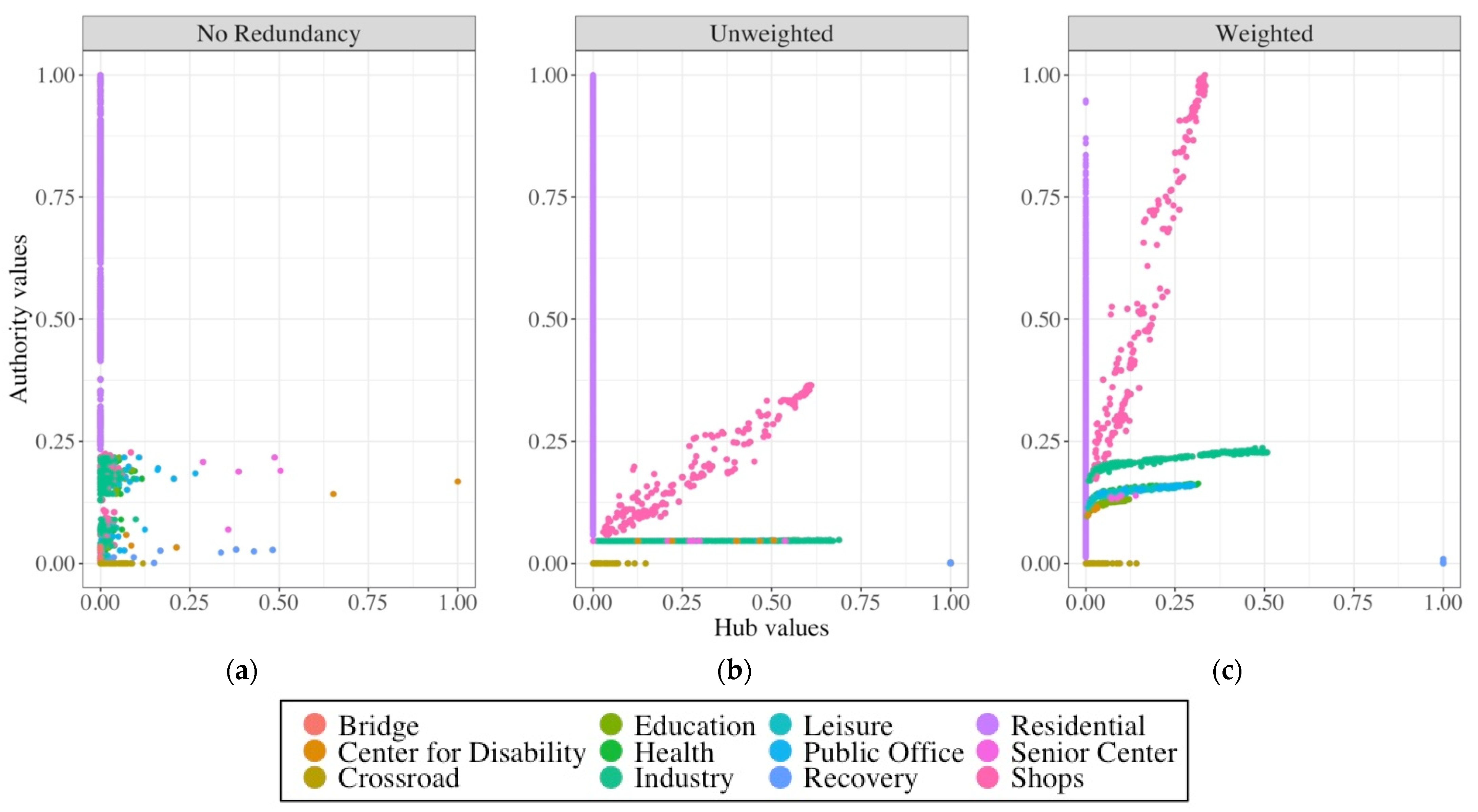
Figure 6 shows the values of hub and authority in three different graph configurations: (1) unweighted graph without services redundancy (i.e., each node receives service from the closest provider); (2) unweighted graph with service redundancy; and (3) weighted graph with service redundancy.
As in the application case of Mexico City [36], these results showed the recovery nodes with higher hub values (i.e., value equal to 1) and the lowest values of authority. The ranking of elements according to their hub values can be very useful for prioritizing intervention actions and maximizing the mitigation effects for the whole network. If an external perturbation hits an element with a very high hub value, the cascading effects on the network will be more relevant due to its central role in the system. On the other hand, a mitigation measure applied to the elements with higher hub values would produce a higher benefit in the whole network. The recovery nodes with the highest hub values confirm the central role of this particular typology of service during a disastrous event.
Regarding the analysis from the receivers’ point of view, we explored how the system privileges some receivers compared with others according to their connections with the providers. In particular, we proposed a comparison between receivers through the authority analysis. In all three configurations, all the residential nodes had hub values equal to zero and distributed authority values from 0 to 1. In the baseline scenario of unweighted graph [37], all the providers had a very narrow range of authority except for the shops; this was due to the structure of the graph; i.e., their authority value was due to their providers (bridge, crossroad, and recovery) which had a very narrow range of hubs. The shops had values that vary according to the hub value of their industrial provider (an industry with a higher value of hub “transfers” higher values to the shops that it serves). On the other hand, if the services were weighted by their own supply capacity, all the services had different authority values. In particular, all providers had higher authority values for higher hub values, and the shops had a greater centrality (i.e., highest values of authority) in the city system; in fact, they had higher values even with respect to the residential nodes, and this was due to the population distribution across the graph by the weighted links.
Figure 7 shows how the authority values change on the territory; we noted that the greater values of authority corresponded to the city center, and going towards the periphery, the values decreased progressively. This result showed in a quantitative manner an intuitively expected output about how an urban area is grown, where the center is richer of services and connections, and vice-versa, in the surrounding areas, they are sparser. To this effect, the authority represents well the exposure system, that particularly privileges some nodes compare to others.
3.2. Assessment of the Resilience
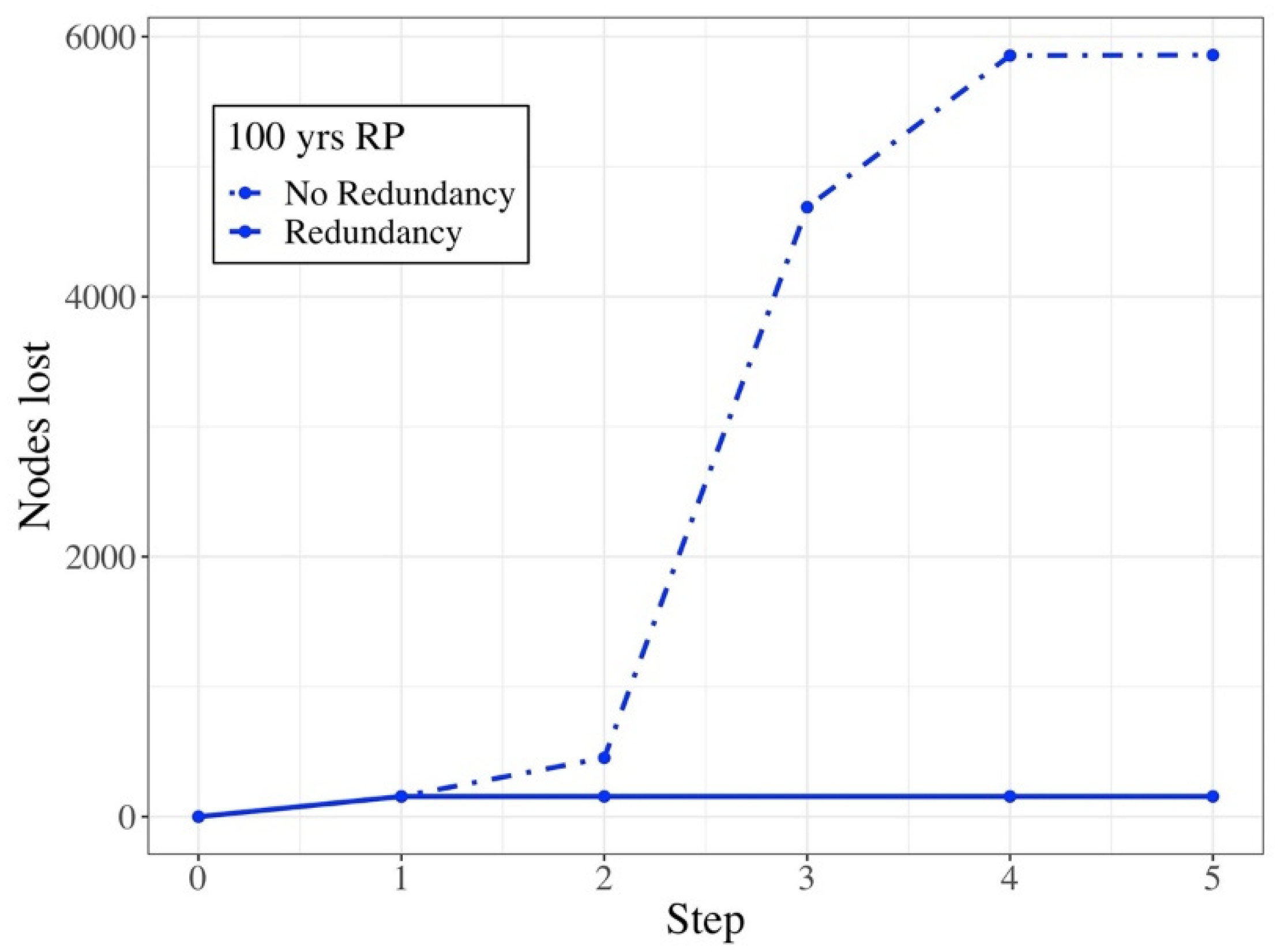
Figure 8 shows the results of the impact of a 100-year return period flood in cases of a graph with and without redundancy. On the x-axis is the number of steps necessary to propagate the impact through the system by the hazard perturbation as described in Section 2.2.2. In fact, step 0 coincides with the system that has not been hit by the hazard, hence, the zero nodes lost. Step 1 is identified by the network as being perturbed by the hazard, and thus the y-axis reports the directly impacted nodes. The subsequent steps are the ones that the system needs to propagate the indirect impact of the flood (i.e., the indirectly hit nodes). It is evident that there is a benefit to redundancy in making the system absorbing the impacts, adapting, and continuing to function in a new configuration, in other words, the system’s resilience. In particular, it can be seen how the configuration of the graph without redundancy (dot-dashed line) let the impact be propagated up to the fifth iteration, reaching several indirectly affected nodes more than 95% of the total. In contrast, in the configuration with redundancy (continuous lines), the propagation ends at the third iteration, indirectly affecting a few units. Every provider’s capacity to absorb new demand and the ability to reallocate service based on the redundancy rules are two aspects that make the system more resilient to an external perturbation.
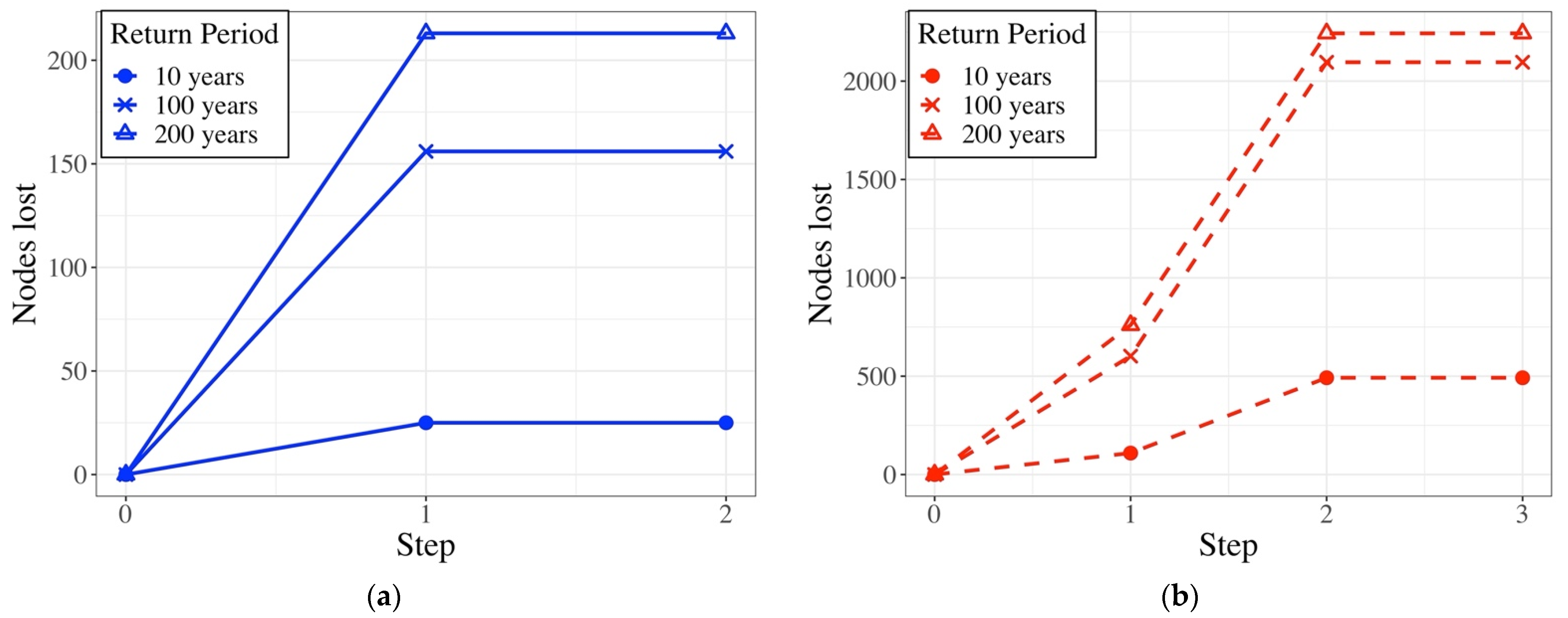
The graph, weighted and constructed considering the redundancy, was perturbed with three return periods (T = 10, T = 100, and T = 200 years) for both hazards, and the results are reported in Figure 9 in terms of impacted nodes.
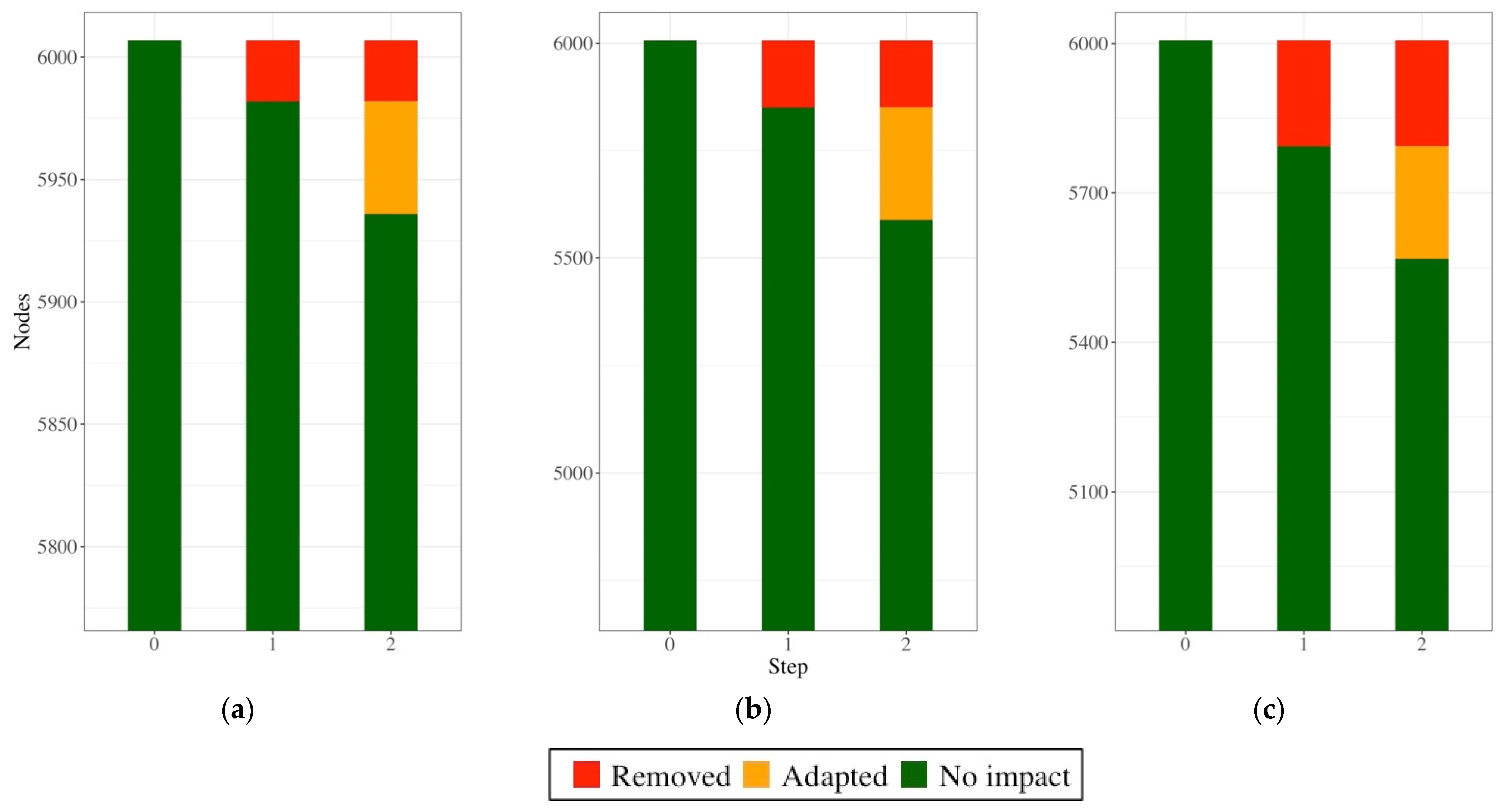
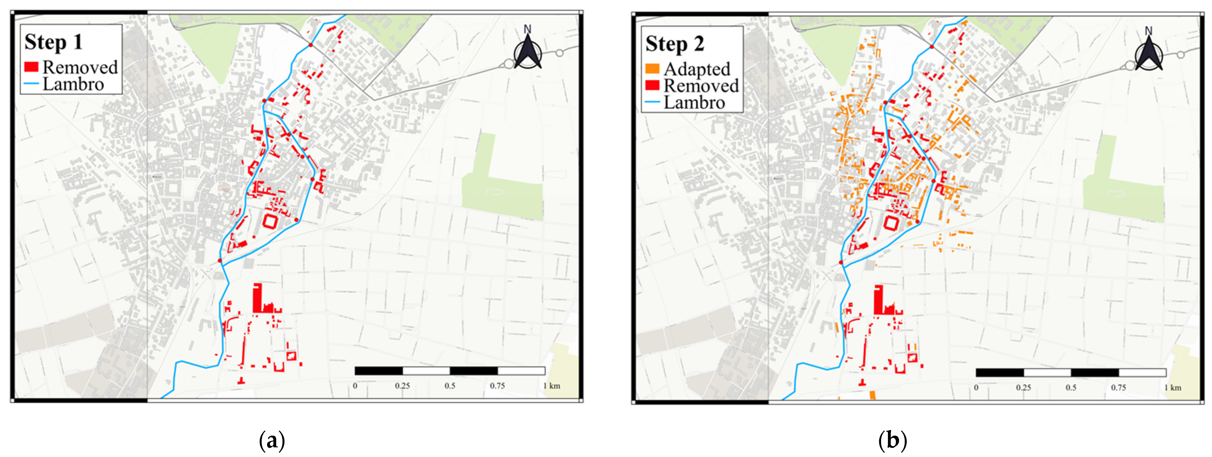
The total number of nodes lost represents only a part of the impact; due to the node directly impacted, nodes are not removed from the graph although affected by a provider’s change (i.e., adapted). Figure 10 shows the number of nodes removed and impacted at each iteration, and Figure 11 shows the same nodes on a map for the river case at T = 100 years.
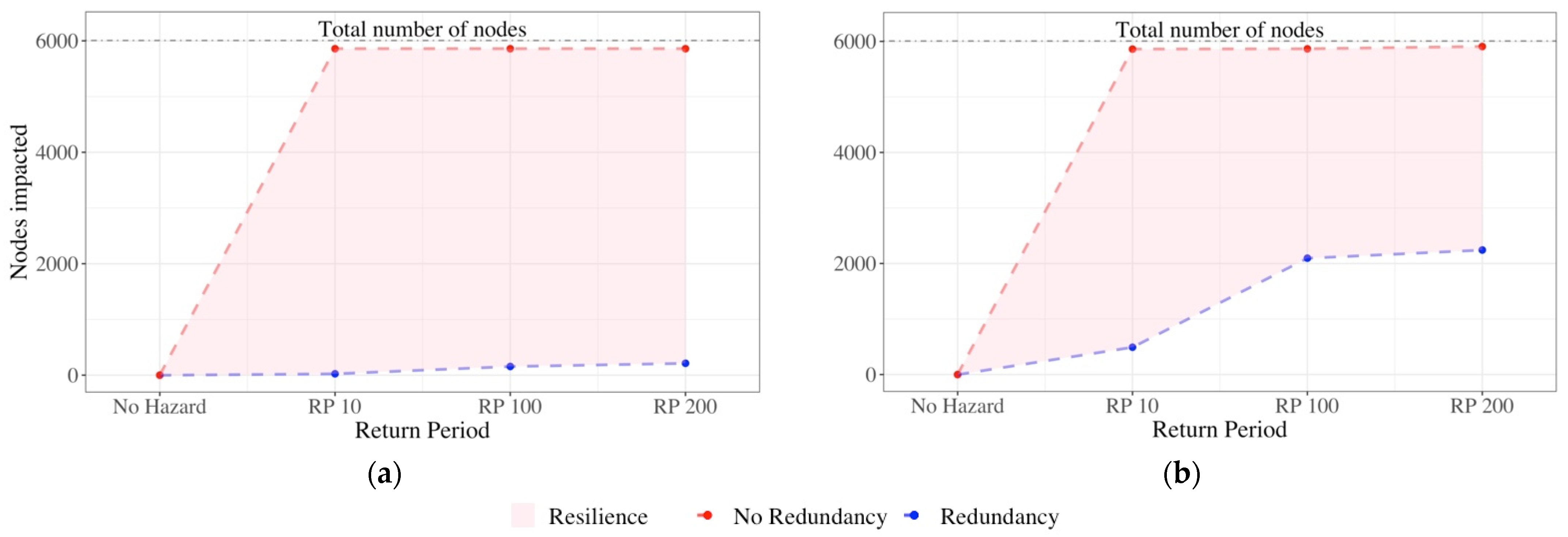
Figure 12 shows the resilience measure represented by the area between the remaining nodes at different return periods in the two propagation scenarios; the first one without considering any capacity to adapt to the perturbation, the second considering the adaptation process reproduced by the services redundancy and the providers’ maximum capacity. In Figure 12, we can observe that the adaptation process is very influential for the total number of nodes affected for both hazards pluvial and fluvial. According to these methods, the resilience was computed as the difference between the annual average loss (i.e., the expected loss per year averaged over many years) of the scenario with and without resilience characteristics. Considering the number of nodes impacted as a loss, for river and pluvial floods, we obtained on average 430 and 548 buildings per year, respectively, not impacted thanks to the resilience properties.
4. Discussion
The methodology presented in this work, although some implementation hypotheses need to be highlighted, showed how to adapt the approach for assessing risk to resilience, proposing a graph construction that reflects the UNGA definition’s resilience characteristics. Some future developments are necessary to make this methodology a useful operative tool for decisionmakers. In particular, the work has introduced significant improvements to the methodology adopted by Arosio et al. (2020) [36,37], both in structural and functional terms.
4.1. Model Assumptions
Simplifications and approximations have been introduced in the methods deployed to connect the nodes. Noticeably, using distance as a criterion, one does not consider the willingness and personal preferences that might lead human beings to go far away from where they live to purchase some goods or services. Besides, in the proposed method, a supplier’s maximum capacity after an event was estimated by adopting a percentage increase in its ordinary capacity. It would be necessary to collect more information on specific services to determine these values with greater accuracy regarding this aspect (e.g., also considering the total quantity of stock). The detailed representation of the categories was not coherent, particularly the transport service (i.e., crossroads and bridges), due to the way the graph was built and the propagation algorithm adopted, containing a lower degree of detail than other services. Finally, in this application, to model the system’s adaptive behavior, the author hypothesized that the impacts’ duration was long enough to give the possibility to the elements to adapt. That may be true for some hazards (e.g., intense earthquakes or particularly destructive floods) and certain services (e.g., education and health) while more difficult for other contexts (e.g., moderate flood).
4.2. Significant Results Achieved
This work showed how to represent most of the UNGA definition’s resilience characteristics: a system that can adapt to, transform, and recover from a hazardous event. Considering these resilience characteristics, a unique quantitative metric for resilience was also proposed by comparing the impact at different hazard return periods for different system configurations. The main results obtained in this work with respect to the previous similar applications [36,37] are:
- Representation improvements of the urban system complexity through a weighted and redundant graph;
- A more accurate assessment of the central elements of the system thanks to the construction of a weighted graph based on the population distribution;
- The construction of a redundant and an adaptable graph that allowed us to reproduce most of the UNGA definition’s resilience characteristics;
- Demonstration that the methodology can assess the resilience to different hazards.
The NEWFRAME project, which funded this research, provided the opportunity to interact with local authorities through a series of meetings, which granted us access to a large amount of information and data that had not been possible in previous applications. That allowed us to consider a list of elements and exchange services. Thus, it was possible to represent, with relative accuracy, the city’s socio-economic system exposed to the risk of flooding. The social characteristics of the population (e.g., age and disability), the distribution of shops, industries, and entertainment venues, together with all the public offices and emergency centers, have well reproduced the city’s complex interaction. The distribution of the people present in various buildings was therefore used to weight the graph and thus be able to distribute the request for services between the various types and the various nodes.
The study of the weighted graph properties showed a different centrality value distribution of the city with respect to the unweighted, highlighting a significantly central role of some shops and industries. The introduction of redundancy also made it possible to highlight the different distribution of services in the graph, which generated higher authority values in the city center, and going towards the periphery, the values decreased progressively.
The adoption of redundant services and the provider capacity made it possible to model an adaptable system that responds dynamically to an external perturbation. These two improvements in the graph construction allow us to better reproduce the generation of indirect impact and, consequently, to assess the total impacts.
Finally, this application shows that this approach is independent from the hazard’s characteristics. Even though the proposed case study considered only two different types of floods, the same global methodology can be adopted also to other hazards, changing the vulnerability function of the first order accordingly, while the following steps of impact propagation and the resilience estimation would not change.
4.3. Future Developments
While application of the methodology to the case study showed that it is possible to apply it to different hazards, a more detailed investigation would require integrating the study of the indirect impact (i.e., propagation) with the one of the direct impact, as estimated by physical vulnerability curves. Indeed, more elaborated curves should describe how the physical damage could trigger the cascade propagation, while, at the moment, only binary vulnerability functions have been adopted (elements can be either impacted or not). In this regard, as highlighted in Arosio 2020 [37], the introduction of the physical vulnerability curves for the nodes directly affected must be accompanied by a second (loss of service provided) and a third (indirect impact to the receiver) level of vulnerability curves. This indeed represents an area of further investigation that requires a more detailed collection of data to improve the quantification of and adaptation to impacts.
Alongside the need for a more elaborate classification of the impacts, the proposed methodology is now limited to three instances: directly impacted, indirectly impacted, and adapted elements. Instead, other quantitative metrics may represent other aspects and intensity of the impact or other side effects generated by the hazard or by the system response (e.g., the costs of adapting the various options, such as the increase in the average distance between suppliers and receivers, number of services interrupted by type).
Finally, it should be emphasized that the graph construction required a large amount of detailed information that it was possible to collect only thanks to the funded project on the city in which the case study was applied. This was undoubtedly an excellent opportunity to test the model and highlight the need to institutionalize databases that contain these particular types of information to expand this type of analysis on larger scales.
Author Contributions
Conceptualization and formal analysis, M.A., L.C. and M.L.V.M.; methodology and software, M.A., L.C. and M.L.V.M.; writing—original draft preparation, M.A., L.C. and M.L.V.M. All authors have read and agreed to the published version of the manuscript.
Funding
This research was funded by Fondazione Cariplo [reference number 2017-0724].
Institutional Review Board Statement
Not applicable.
Informed Consent Statement
Not applicable.
Data Availability Statement
Restrictions apply to the availability of these data. Data were obtained from Comune di Monza and are not publicly available due to privacy reason.
Acknowledgments
This research was partly funded by Fondazione Cariplo under the project “NEWFRAME: NEtWork-based Flood Risk Assessment and Management of Emergencies”, and it has been developed within the framework of the project “Dipartimenti di Eccellenza”, funded by the Italian Ministry of Education, University and Research at IUSS Pavia. We thank Regione Lombardia for the support within the project “Ripresa Economica” for the realization of a HPC Data Center at IUSS.
Conflicts of Interest
The authors declare no conflict of interest.
Appendix A. Characteristics of the City Building
Table A1 reports the characteristics of each city building as provided by the municipality of Monza.

Table A1.
Description of the features of the exposure dataset of the city of Monza.
| Feature | Description |
|---|---|
| ID | A univocal alpha-numeric code that identifies the building |
| Height | Minimum height above sea level of the building [m] |
| Max_height | Maximum height above sea level of the building [m] |
| Rel_height | Relative height of the building obtained as Max_height—height [m] |
| Area | Area of the shapefile representing the building |
| Volume | Volume of the building obtained as the product between Area and Rel_height |
| Address | Address at which the building is registered in the municipality archive |
| Year_of_construction | The time interval during which the building was constructed. |
| State_of_conservation | Indicates the current state of conservation of the building. Three categories were given: Excellent, Good, Bad. |
| Type_building | Indicates the type of construction among masonry, reinforced concrete, and others. The latter comprises wood, steel, and other types of construction that are less frequent in the historical center of an Italian city |
| Destination_use | Indicates the activity and the destination of use of the building. The categories are reported in Table 2. |
| Number_families | Reports the number of families living in the building |
| Number_residents | Reports the number of residents living in the building |
| Number_disabled | Reports the number of disabled people living in the building |
References
- Cutter, S.L.; Ash, K.D.; Emrich, C.T. The geographies of community disaster resilience. Glob. Environ. Chang. 2014, 29, 65–77. [Google Scholar] [CrossRef]
- Klein, R.J.T.; Nicholls, R.J.; Thomalla, F. Resilience to Natural Hazards: How Useful Is This Concept? Glob. Environ. Chang. Part B Environ. Hazards 2004, 5, 35–45. [Google Scholar] [CrossRef]
- Zhou, H.; Wang, J.; Wan, J.; Jia, H. Resilience to natural hazards: A geographic perspective. Nat. Hazards 2010, 53, 21–41. [Google Scholar] [CrossRef]
- Alexander, D.E. Resilience and disaster risk reduction: An etymological journey. Nat. Hazards Earth Syst. Sci. 2013, 13, 2707–2716. [Google Scholar] [CrossRef] [Green Version]
- Burton, C.G. A Validation of Metrics for Community Resilience to Natural Hazards and Disasters Using the Recovery from Hurricane Katrina as a Case Study. Ann. Assoc. Am. Geogr. 2015, 105, 67–86. [Google Scholar] [CrossRef]
- Timmerman, P. Vulnerability, resilience and the collapse ofsociety. In A Review of Models and Possible Climatic Applications; Institute for Environmental Studies, University of Toronto: Toronto, ON, Canada, 1981. [Google Scholar]
- Adger, W.N. Social and ecological resilience: Are they related? Prog. Hum. Geogr. 2000, 24, 347–364. [Google Scholar] [CrossRef]
- Torres, J. Crossing Borders: A Comparative Assessment of Community Resilience to Natural Hazards in Arica and Parinacota (Chile) and Tacna (Peru) Regions; Istituto Universitario di Studi Superiori di Pavia Crossing: Pavia, Italy, 2020. [Google Scholar]
- Nation, U. Sendai Framework for Disaster Risk Reduction 2015–2030; UNDRR: Geneva, Switzerland, 2015. [Google Scholar]
- Bruneau, M.; Chang, S.E.; Eguchi, R.T.; Lee, G.C.; O’Rourke, T.D.; Reinhorn, A.M.; Shinozuka, M.; Tierney, K.; Wallace, W.A.; Von Winterfeldt, D. A Framework to Quantitatively Assess and Enhance the Seismic Resilience of Communities. Earthq. Spectra 2003, 19, 733–752. [Google Scholar] [CrossRef] [Green Version]
- Burton, C.G. The Development of Metrics for Community Resilience to Natural Disasters. Ph.D. Thesis, University of South Carolina, Columbia, SC, USA, 2012; p. 198. [Google Scholar] [CrossRef]
- Cumming, G.S.; Barnes, G.; Perz, S.; Schmink, M.; Sieving, K.E.; Southworth, J.; Binford, M.; Holt, R.D.; Stickler, C.; Van Holt, T. An exploratory framework for the empirical measurement of resilience. Ecosystems 2005, 8, 975–987. [Google Scholar] [CrossRef]
- Cutter, S.L.; Barnes, L.; Berry, M.; Burton, C.; Evans, E.; Tate, E.; Webb, J. A place-based model for understanding community resilience to natural disasters. Glob. Environ. Chang. 2008, 18, 598–606. [Google Scholar] [CrossRef]
- Cutter, S.L.; Burton, C.G.; Emrich, C.T. Journal of Homeland Security and Disaster Resilience Indicators for Benchmarking Baseline Conditions Disaster Resilience Indicators for Benchmarking Baseline Conditions. J. Homel. Secur. Emerg. Manag. 2010, 7. [Google Scholar] [CrossRef]
- Francis, R.; Bekera, B. A Metric and Frameworks for Resilience Analysis of Engineered and Infrastructure Systems; Elsevier: Amsterdam, The Netherlands, 2014; Volume 121, ISBN 1202994024. [Google Scholar]
- Peacock, W. Advancing the Resilience of Coastal Localities: Developing, Implementing and Sustaining the Use of Coastal Resilience Indicators: A Final Report. Hazard Reduct. Recovery Cent. 2010. [Google Scholar] [CrossRef]
- Sherrieb, K.; Norris, F.H.; Galea, S. Measuring Capacities for Community Resilience. Soc. Indic. Res. 2010, 99, 227–247. [Google Scholar] [CrossRef]
- Lam, N.N.S.; Reams, M.; Li, K.; Li, C.; Mata, L.P. Measuring Community Resilience to Coastal Hazards along the Northern Gulf of Mexico. Nat. Hazards Rev. 2016, 17, 04015013. [Google Scholar] [CrossRef] [Green Version]
- Zimmerman, R. Social Implications of Infrastructure Network Interactions. J. Urban Technol. 2001, 8, 97–119. [Google Scholar] [CrossRef]
- Tierney, K.J. Conceptualizing and Measuring Organizational and Community Resilience: Lessons from the Emergency Response Following the 11 September 2001 Attack on the World Trade Center; Disaster Research Center: Columbus, OH, USA, 2003. [Google Scholar]
- David, R. Godschalk Urban Hazard Mitigation: Creating Resilient Cities. Nat. Hazards Rev. 2003, 4, 136–143. [Google Scholar] [CrossRef]
- Arup, T.R.F. City Resilience Framework; The Rockefeller Foundation: London, UK, 2015. [Google Scholar]
- UNDRR. Disaster Resilience Scorecard for Cities—Preliminary Level Assessment; UNDRR: Geneva, Switzerland, 2017. [Google Scholar]
- WCCD. ISO 37120 Sustainable Development of Communities: Indicators for City Services and Quality of Life; WCCD: Detroit, MI, USA, 2014. [Google Scholar]
- Zampieri, M. Reconciling the ecological and engineering definitions of resilience. Ecosphere 2021, 12, e03375. [Google Scholar] [CrossRef]
- Morecroft, M.D.; Crick, H.Q.P.; Duffield, S.J.; Macgregor, N.A. Resilience to climate change: Translating principles into practice. J. Appl. Ecol. 2012, 49, 547–551. [Google Scholar] [CrossRef]
- Quinlan, A.E.; Berbés-Blázquez, M.; Haider, L.J.; Peterson, G.D. Measuring and assessing resilience: Broadening understanding through multiple disciplinary perspectives. J. Appl. Ecol. 2016, 53, 677–687. [Google Scholar] [CrossRef]
- Scheffer, M.; Carpenter, S.R.; Dakos, V.; van Nes, E.H. Generic Indicators of Ecological Resilience: Inferring the Chance of a Critical Transition. Annu. Rev. Ecol. Evol. Syst. 2015, 46, 145–167. [Google Scholar] [CrossRef]
- Jones, L. Resilience isn’t the same for all: Comparing subjective and objective approaches to resilience measurement. Wiley Interdiscip. Rev. Clim. Chang. 2019, 10, 1–19. [Google Scholar] [CrossRef] [Green Version]
- UN Secretary-General (A/71/276). Report of the Open-Ended Intergovernmental Expert Working Group on Indicators and Terminology Relating to Disaster Risk Reduction; United Nations General Assembly: New York, NY, USA, 2017; Volume 8, pp. 49–116. [Google Scholar]
- UN Secretary-General A/71/644. Report of the Open-Ended Intergovernmental Expert Working Group on Indicators and Terminology Relating to Disaster Risk Reduction; United Nations General Assembly: New York, NY, USA, 2016; Volume 21184, pp. 1–41. [Google Scholar]
- Metzger, P.; Robert, J.; Área, P.F. Elementos de reflexión sobre la resiliencia urbana: Usos criticables y aportes potenciales. Territories 2013, 28, 21–40. [Google Scholar]
- Clark-Ginsberg, A.; Abolhassani, L.; Rahmati, E.A. Comparing networked and linear risk assessments: From theory to evidence. Int. J. Disaster Risk Reduct. 2018, 30, 216–224. [Google Scholar] [CrossRef]
- Lee, K. Appraising Adaptive Management. Biol. Divers 2001, 3, 3–26. [Google Scholar] [CrossRef] [Green Version]
- von Bertalanffy, L. An outline of general system theory. Br. J. Philos. Sci. 1950, 1, 134–165. [Google Scholar] [CrossRef]
- Arosio, M.; Martina, M.L.V.; Figueiredo, R. The whole is greater than the sum of its parts: A holistic graph-based assessment approach for natural hazard risk of complex systems. Nat. Hazards Earth Syst. Sci. 2020, 20, 521–547. [Google Scholar] [CrossRef] [Green Version]
- Arosio, M.; Martina, M.L.V.; Creaco, E.; Figueiredo, R. Indirect Impact Assessment of Pluvial Flooding in Urban Areas Using a Graph-Based Approach: The Mexico City Case Study. Water 2020, 12, 1753. [Google Scholar] [CrossRef]
- Fekete, A. Critical infrastructure and flood resilience: Cascading effects beyond water. Wiley Interdiscip. Rev. Water 2019, 6, e1370. [Google Scholar] [CrossRef] [Green Version]
- Fekete, A. Common criteria for the assessment of critical infrastructures. Int. J. Disaster Risk Sci. 2011, 2, 15–24. [Google Scholar] [CrossRef] [Green Version]
- Buldyrev, S.V.; Parshani, R.; Paul, G.; Stanley, H.E.; Havlin, S. Catastrophic cascade of failures in interdependent networks. Nature 2010, 464, 1025–1028. [Google Scholar] [CrossRef] [Green Version]
- Rinaldi, S.M.; Peerenboom, J.P.; Kelly, T.K. Identifying, understanding, and analyzing critical infrastructure interdependencies. IEEE Control Syst. Mag. 2001, 21, 11–25. [Google Scholar] [CrossRef]
- Zorn, C.; Pant, R.; Thacker, S.; Shamseldin, A.Y. Evaluating the magnitude and spatial extent of disruptions across interdependent national infrastructure networks. ASCE-ASME J. Risk Uncertain. Eng. Syst. Part. B Mech. Eng. 2020, 6. [Google Scholar] [CrossRef]
- Roy, K.C.; Hasan, S.; Mozumder, P. A multilabel classification approach to identify hurricane-induced infrastructure disruptions using social media data. Comput.-Aided Civil Infrastruct. Eng. 2020, 35, 1387–1402. [Google Scholar] [CrossRef]
- Papilloud, T.; Röthlisberger, V.; Loreti, S.; Keiler, M. Flood exposure analysis of road infrastructure—Comparison of different methods at national level. Int. J. Disaster Risk Reduct. 2020, 47, 101548. [Google Scholar] [CrossRef]
- Arrighi, C.; Pregnolato, M.; Castelli, F. Indirect flood impacts and cascade risk across interdependent linear infrastructures. Nat. Hazards Earth Syst. Sci. 2020, 21, 1955–1969. [Google Scholar] [CrossRef]
- Pant, R.; Thacker, S.; Hall, J.W.; Alderson, D.; Barr, S. Critical infrastructure impact assessment due to flood exposure. J. Flood Risk Manag. 2018, 11, 22–33. [Google Scholar] [CrossRef]
- Koks, E.; Pant, R.; Thacker, S.; Hall, J.W. Understanding Business Disruption and Economic Losses Due to Electricity Failures and Flooding. Int. J. Disaster Risk Sci. 2019, 10, 421–438. [Google Scholar] [CrossRef] [Green Version]
- Boccaletti, S.; Latora, V.; Moreno, Y.; Chavez, M.; Hwang, D.U. Complex networks: Structure and dynamics. Phys. Rep. 2006, 424, 175–308. [Google Scholar] [CrossRef]
- Börner, K.; Soma, S.; Vespignani, A. Network Science. Annu. Rev. Inf. Technol. 2007, 41, 537–607. [Google Scholar] [CrossRef]
- Nepusz, T.; Csard, G. Package “igraph”—Network Analysis and Visualization. Available online: https://cran.r-project.org/web/packages/igraph/igraph.pdf (accessed on 11 September 2021).
- Biggs, N.L.; Lloyd, E.K.; Wilson, R.J. Graph. Theory 1736–1936; Clarendon Press: Oxford, UK, 1976. [Google Scholar]
- Barabasi, A.L. Network Science. Available online: http://barabasi.com/networksciencebook/ (accessed on 11 September 2021).
- Newman, M.E.J. Networks An. Introduction; Springer Science & Business Media: Oxford, UK; New York, NY, USA, 2010; ISBN 9780199206650. [Google Scholar]
- Koenig, M.D.; Battiston, S. From Graph Theory to Models of Economic Networks. A Tutorial. In Networks, Topology and Dynamics; Springer: Berlin, Germany, 2009; pp. 23–63. ISBN 978-3-540-68407-7. [Google Scholar]
- Galuppini, G.; Quintilliani, C.; Arosio, M.; Barbero, G.; Ghilardi, P.; Manenti, S.; Petaccia, G.; Todeschini, S.; Ciaponi, C.; Martina, M.L.V.; et al. A unified framework for the assessment of multiple source urban flash flood hazard: The case study of Monza, Italy. Urban. Water J. 2020, 17, 65–77. [Google Scholar] [CrossRef]
Figure 1.
Conceptual propagation of the direct and indirect impacts in a system under probability scenario event of T = 200.
Figure 1.
Conceptual propagation of the direct and indirect impacts in a system under probability scenario event of T = 200.

Figure 2.
(a) Comparison of total impact between a static graph and a graph with the resilience characteristics. (b) Resilience representation as the area between the risk curve computed for a static graph and a graph with the resilience characteristics.
Figure 2.
(a) Comparison of total impact between a static graph and a graph with the resilience characteristics. (b) Resilience representation as the area between the risk curve computed for a static graph and a graph with the resilience characteristics.

Figure 3.
An illustrative example shows the two improvements introduced in the graph building (service redundant and weighted graph): (a) non-redundant and unweighted graph (each node receives a service only from the closest providers); (b) redundant and unweighted graph (each node provides services to all the receivers within a radius r); (c) redundant and weighted graph (to each link, the number of users that the link serves is assigned).

Figure 4.
High-level description of the propagation process.

Figure 5.
Map of providers (left) and services (right) exchange between themselves (case: no redundancy, the connections and providers to residential receivers were removed for readability).
Figure 5.
Map of providers (left) and services (right) exchange between themselves (case: no redundancy, the connections and providers to residential receivers were removed for readability).

Figure 6.
Plot authority versus hub for the three different graph configurations: (a) no redundancy; (b) redundancy unweighted, and (c) redundancy weighted.
Figure 6.
Plot authority versus hub for the three different graph configurations: (a) no redundancy; (b) redundancy unweighted, and (c) redundancy weighted.

Figure 7.
Map of the authority values.

Figure 8.
Impact propagations: comparison between a non-redundant and redundant graph (river scenario).
Figure 8.
Impact propagations: comparison between a non-redundant and redundant graph (river scenario).

Figure 9.
Impact propagations for different return periods: (a) fluvial scenarios and (b) pluvial scenarios.
Figure 9.
Impact propagations for different return periods: (a) fluvial scenarios and (b) pluvial scenarios.

Figure 10.
The number of nodes that are impacted at different iterations for river flood: (a) 10 years RP; (b) 100 years RP; (c) 200 years RP.
Figure 10.
The number of nodes that are impacted at different iterations for river flood: (a) 10 years RP; (b) 100 years RP; (c) 200 years RP.

Figure 11.
Map of buildings impacted in the river scenario at T = 100 years: (a) directly impacted (step 1); (b) indirectly impacted (step 2).
Figure 11.
Map of buildings impacted in the river scenario at T = 100 years: (a) directly impacted (step 1); (b) indirectly impacted (step 2).

Figure 12.
Representation of the resilience as the difference between adaptable and redundant graph respect to the static and non-redundant graph: in the case of (a) the river and (b) pluvial scenarios.
Figure 12.
Representation of the resilience as the difference between adaptable and redundant graph respect to the static and non-redundant graph: in the case of (a) the river and (b) pluvial scenarios.

Table 1.
Types of impacts.
| Physical Damages | Non-Physical Damages | |
|---|---|---|
| Elements directly impacted | (a) Physical damages directly due to the event (Vulnerability of the first order) | (b) Non-physical damages due to the physical damages (Vulnerability of the second order) |
| Elements indirectly impacted | (c) Non-physical damages due to the interruption of the service provided by an impacted node (Vulnerability of the third order) |
Table 2.
List of node types.
| Category of Node | Number | The Receiver of the Service |
|---|---|---|
| Bridge | 10 | Crossroad |
| Center for Disability | 6 | Residential |
| Crossroad | 50 | All Typology |
| Education | 136 | Residential |
| Health | 80 | Residential |
| Industry | 331 | Residential, Shops |
| Leisure | 143 | Residential |
| Public Office | 28 | Residential |
| Recovery | 10 | All typology except for Bridge and Crossroad |
| Senior Center | 6 | Residential |
| Shops | 214 | Residential |
| Residential | 4990 | None |
Table 3.
Spatial ranges employed for establishing connections.
| Provider | Receiver | Spatial Range |
|---|---|---|
| Bridge | Crossroad | Parallel Bands |
| Center for Disability | Residential | Radial Area |
| Crossroad | All Typology | Radial Area |
| Education | Residential | Radial Area |
| Health | Residential | Radial Area |
| Industry | Residential, Shops | Radial Area |
| Leisure | Residential | Radial Area |
| Public Office | Residential | Radial Area |
| Recovery | All typology except for Bridge and Crossroad | Entire City |
| Senior Center | Residential | Radial Area |
| Shops | Residential | Radial Area |
Publisher’s Note: MDPI stays neutral with regard to jurisdictional claims in published maps and institutional affiliations. |
© 2021 by the authors. Licensee MDPI, Basel, Switzerland. This article is an open access article distributed under the terms and conditions of the Creative Commons Attribution (CC BY) license (https://creativecommons.org/licenses/by/4.0/).
Share and Cite
MDPI and ACS Style
Arosio, M.; Cesarini, L.; Martina, M.L.V. Assessment of the Disaster Resilience of Complex Systems: The Case of the Flood Resilience of a Densely Populated City. Water 2021, 13, 2830. https://doi.org/10.3390/w13202830
AMA Style
Arosio M, Cesarini L, Martina MLV. Assessment of the Disaster Resilience of Complex Systems: The Case of the Flood Resilience of a Densely Populated City. Water. 2021; 13(20):2830. https://doi.org/10.3390/w13202830
Chicago/Turabian StyleArosio, Marcello, Luigi Cesarini, and Mario L. V. Martina. 2021. "Assessment of the Disaster Resilience of Complex Systems: The Case of the Flood Resilience of a Densely Populated City" Water 13, no. 20: 2830. https://doi.org/10.3390/w13202830
Note that from the first issue of 2016, this journal uses article numbers instead of page numbers. See further details here.