
Large-Volume Samplers for Efficient Composite Sampling and Particle Characterization in Sewer Systems


Department of Aquatic Environmental Engineering, Institute for Water and River Basin Management, Karlsruhe Institute of Technology (KIT), Gotthard-Franz-Str. 3, 76131 Karlsruhe, Germany
*
Authors to whom correspondence should be addressed.
Water 2021, 13(20), 2831; https://doi.org/10.3390/w13202831
Submission received: 7 September 2021
/
Revised: 6 October 2021
/
Accepted: 8 October 2021
/
Published: 12 October 2021
(This article belongs to the Special Issue Monitoring, Modelling and Management of Water Quality II)
Abstract
:The assessment of pollution from sewer discharges requires flexible and reliable sampling methods. The characteristics of the sampling system must be known to allow comparison with other studies. Large volume samplers (LVS) are increasingly used for monitoring in sewer systems and surface waters. This article provides a comprehensive description of this widely applicable sampling system, gives insight into its comparability to standard methods, and provides recommendations for researchers and practitioners involved in water quality monitoring and urban water management. Two methods for subsampling from LVS are presented, i.e., collection of homogenized or sedimented samples. Results from a sampling campaign at combined sewer overflows (CSOs) were used to investigate the comparability of both subsampling methods and conventional autosamplers (AS). Event mean concentrations (EMC) of total suspended solids (TSS) derived from homogenized LVS samples and AS pollutographs were comparable. TSS-EMC of homogenized and sedimented LVS samples were also comparable. However, differences were found for particle size distribution and organic matter content. Consequently, sedimented LVS samples, which contained solids masses in the range of 3–70 g, are recommended to be used for particle characterization. The differences between homogenized and sedimented LVS samples, e.g., the quality of homogenization and the stability of samples during sedimentation in LVS, should be further investigated. Based on LVS results, average TSS concentrations of 50–60 mg/L were found for CSOs from centralized treatment facilities in Bavaria. With a median share of 84%, particles <63 µm were the dominant fraction.
1. Introduction
Discharges from sewer systems contribute significantly to the total pollutant load to receiving water bodies [1,2,3,4,5]. The monitoring of stormwater runoff and combined sewer overflows (CSOs) has become increasingly important for better quantifying these contributions and for developing effective strategies to reduce pollutant emissions.
Solids play a key role for water quality management. They impact the physical, chemical, and biological properties of water bodies and represent a transport matrix for adsorbed pollutants [6]. Consequently, total suspended solids (TSS) are among the most frequently measured parameters in stormwater monitoring [7] and are often used as a proxy for overall water quality in urban drainage modeling [8]. The environmental fate of suspended solids and the magnitude of their effects in aquatic ecosystems depend on their properties, e.g., particle size distribution (PSD) and chemical composition [6]. Knowledge of these properties is necessary for assessing the origin, the significance to water quality, and the treatability of suspended solids for effective modeling and for designing effective stormwater management measures [7,8,9,10,11].
Due to highly variable flow conditions and fluctuating concentrations, the sampling time in a storm event is decisive for representative quality assessment [12]. Two main strategies for sampling storm events are to collect either discrete single samples distributed across an event [13,14,15,16] or one composite sample representative of the entire discharge period [4,5]. Both the pollutograph produced from single samples and a composite sample can be used to quantify the event mean concentrations (EMC) [17,18]. Generally, events should be sampled as completely as possible to avoid over- or underestimation of EMC. Composite sampling lacks time-resolved information but is advantageous in sampling entire event durations while reducing analytical costs [19].
Large-volume samplers (LVS) are composite samplers with increased capacity of up to 1000 L. The high volume gives flexibility in capturing long-duration and high-volume events while maintaining a sufficiently representative subsample volume of several liters. Particularly, the amount of solids collected in the sampler enables further particle analyses to be carried out [20].
LVSs were first developed in the late 2000s as a method for improving the quality of particle analyses by collecting high solids masses. They have since been used for monitoring street runoff [21], stormwater discharges in separate sewer systems [22,23], combined sewer overflows [20,24,25], and surface waters [26,27,28]. However, the comparability with other sampling methods has not been investigated so far.
The objectives of this article are (1) to provide a comprehensive description of LVS and two methods for subsampling from LVS composite samples (i.e., collection of homogenized samples and sedimented samples) and (2) to evaluate the results of a CSO sampling campaign [29] with simultaneous use of LVS and conventional autosamplers (AS). The comparability of the TSS-EMC derived from both sampling systems was investigated. Furthermore, both LVS subsampling methods were applied to the same original samples to investigate the influence of subsampling on the quantification of TSS and the concentration of total suspended solids < 63 µm (TSS63). TSS63 were recently introduced as a new regulatory parameter for stormwater treatment in Germany [30]. The clay and silt-sized solids have been identified as the dominant particle size fraction in stormwater runoff following wash-off from impervious surfaces due to hydraulic sorting [31]. Larger particles have a lower wash-off mobility and are more likely to be retained on surfaces [32]. In addition, larger particles are preferentially deposited during transport in the sewer system depending on flow conditions [7,33]. With TSS63, which are not biased by larger particles, a better comparability of the results of different sites is achieved. Furthermore, fine particles are associated with high pollutant loading [23,34,35,36] and represent the most critical fraction to physical separation processes common in stormwater treatment, i.e., sedimentation or filtration [33,37]. Our analyses are considered important to better understand the comparability of monitoring results produced with LVS. In addition, the results provide new data on the concentrations, organic matter content, and pollutant loading of solids in CSOs.
2. Materials and Methods
2.1. Large-Volume Samplers
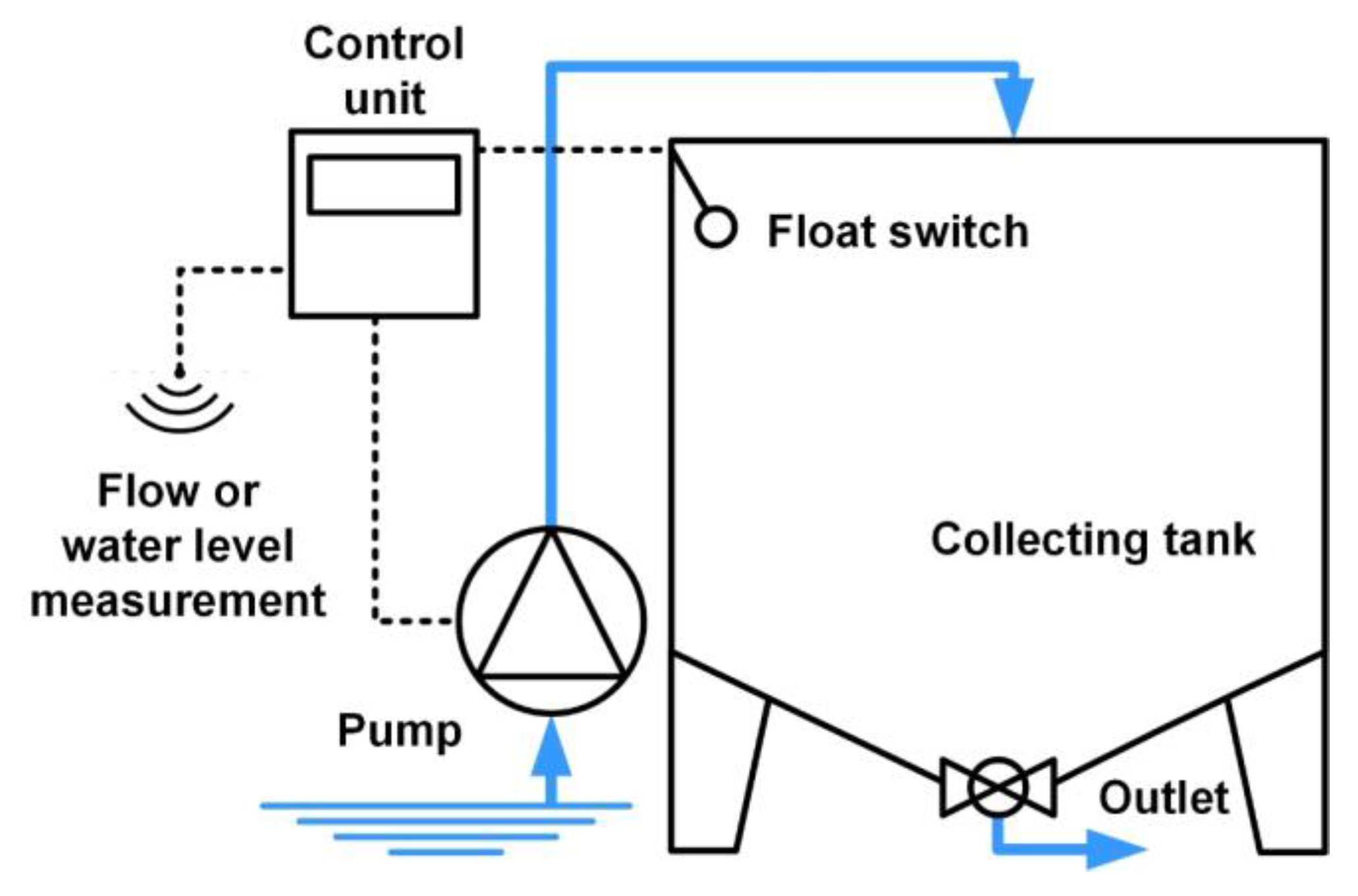
LVS were designed to collect long-term or event-based volume-proportional composite samples and to collect sufficient solids masses to allow reliable quantification and particle characterization, e.g., PSD and chemical composition. For this purpose, large collecting tanks of up to 1000 L, powerful pumps with capacities ≥1000 L∙h−1, and tubings with diameters of 19–25 mm are used. The general setup is shown in Figure 1. A control unit processes water level or flow measurement signals to integrate the discharge volume at the sampling site. The sampling pump is activated at defined volume intervals. The specific duration of one pumping action defines the subsample volume. Different setups of LVS have been used and adapted to specific research objectives, e.g., glass–fiber reinforced plastic tanks were replaced by stainless steel tanks to provide a sampling container with minimized ad- or desorption effects suitable for the quantification of micropollutants [25]. In another study, a three-way valve was installed before the tank inlet to realize a flushing of the tubing system prior to sampling [26]. Assuming a TSS concentration range of 10–1000 mg/L and a LVS sample volume of 100–1000 L, the total dry mass in the tank may range from 1 to 1000 g.
2.2. Subsampling Methods
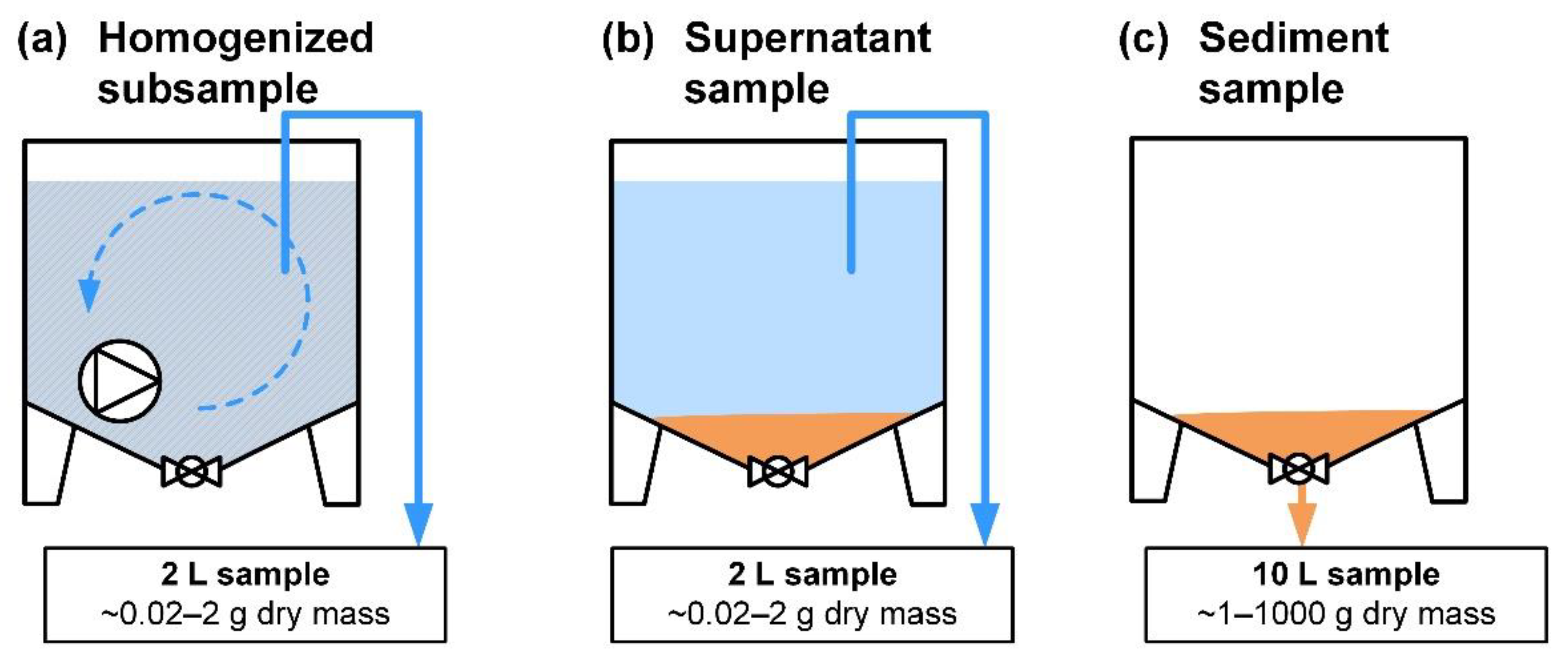
On completion of a sampling period, there are two methods for subsampling the large-volume composite samples from the collecting tank (Figure 2).
2.2.1. Homogenized Sample
Homogenized subsamples of the total composite sample are used to quantify total concentrations of pollutants [25]. After the sampling period, sediments and suspended solids in the container are homogenized by using a submersible pump to agitate the sample (Figure 2a). After several minutes, 2 L subsamples are collected. From the total dry mass calculated above, approximately 0.02–2 g are sampled for analysis. This method is fast and easy to carry out.
2.2.2. Sedimented Sample with Supernatant Sample
Sedimented samples are used for particle analyses and for quantifying loads based on high solids masses [22,24]. For this purpose, composite samples are left to settle for 1–2 days until settling is completed, according to visual inspection. Considering particle settling velocity distributions of combined sewage reported in the literature [38], e.g., [39], all settleable solids should settle in the tank within one day. Grab samples from the supernatant water are collected (Figure 2b) to quantify the remaining suspended solids concentration, or to analyze dissolved substances. From a bottom valve, the first flush of sediments is collected into a 10 L sampling container before the supernatant water is drained at low speed to avoid flushing of sediments. Afterwards, all remaining sediments are mobilized using supernatant water and quantitatively collected in a 10 L sampling container (Figure 2c). In this way, the complete dry mass is sampled for analysis.
2.3. Sampling Campaign
In a study on CSO quality in Bavaria, ten CSO facilities were investigated with regard to different objectives [29]. To assess EMC, homogenized LVS samples were collected at all sites. Autosamplers were used to assess concentration dynamics at selected CSOs (SED02, SED05, SES02). At two CSOs from sedimentation facilities, additional LVS samples were taken from the inlet to estimate sedimentation efficiency (SED02, SED06). For a robust quantification of the TSS load and for conducting particle analyses, sedimented LVS samples were used at these two sites and one additional CSO (FFR02). For the present evaluation, those datasets were selected in which different sampling techniques were used simultaneously (Table 1). The five CSOs considered were all CSOs from centralized stormwater tanks with storage volumes of 10–30 m3∙ha−1. Samples were collected either directly at the inlet or overflow weir, or in the sewer connecting CSO and receiving water (Figures S1–S5).
Each sampling was intended to capture one discrete event, which was defined as the overflow occurring during the period from filling to emptying of the storage volume. In few cases, multiple consecutive events were combined into one composite sample because the sample containers could not be emptied in time. AS were programmed to collect 18 min composite samples in each of the 12 bottles at the sites SED02 and SED05, and 15 min composite samples in 24 bottles at SES02. The maximum sampling duration was 3.6 and 6 h, respectively. LVS sampling intervals were adjusted so that high-volume events could also be sampled before the collecting tank was filled (Table 1). Figure 3 shows the LVS setup used in the study.
2.4. Analytical Methods
2.4.1. Standard Water Quality Parameters
AS samples and homogenized LVS samples were analyzed for pH, conductivity, and concentrations of TSS, chemical oxygen demand (COD), total nitrogen bound (TNb), and total phosphorus (TP) using standard methods (Table S1). Additionally, homogenized LVS samples were analyzed for phosphate-phosphorus (PO4-P).
2.4.2. Particle Size Fractionation and Loss on Ignition
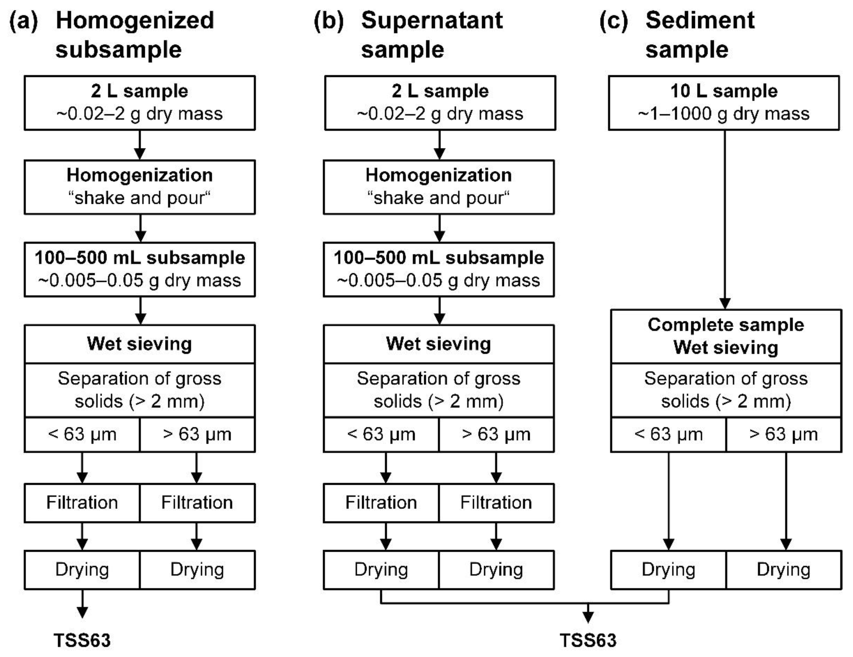
For both homogenized and sedimented LVS samples, wet sieving was used to separate TSS63 and TSS 63–2000 µm. Since sample volume and solids content differed significantly between the sample types, different analytical methods were required.
For the analysis of TSS in homogenized water samples by means of filtration (Figure 4a), further subsampling was needed to yield an appropriate filtered mass in the range of 5–50 mg [40]. To ensure representative subsampling, homogenization was required. This was done by manual shaking. Subsequently, wet sieving was conducted at mesh sizes of 2 mm and 63 µm. Solids >2 mm were separated to avoid bias from coarse solids that are not reliably sampled by most sampling devices [41]. For filtration, glass fiber filters (Macherey-Nagel MN 85/70) with an average pore size of 0.6 µm were used. The boundary to the dissolved fraction was defined at 0.45 µm by using membrane filters for filtration. However, in practice, glass fiber filters are prevalently used because they are resistant to clogging, even if samples have a high organic content. Differences are considered negligible [42]. The filters were dried for at least 1–2 h at 105 °C until constant weight. The loss on ignition (LOI) was determined after heating the filters at 550 °C until constant weight.
Contrastingly, the sedimented samples of approximately 10 L (Figure 4c) contained all solids from the respective composite sample, e.g., around 1–100 g in CSO. The total sample was subjected to wet sieving. Afterwards, the individual particle size fractions were dried at 105 °C. A dry mass of at least 0.1 g of a fraction is required for reliable quantification. The fine fraction <63 μm was thickened to a maximum of 1–1.5 L before drying by decanting the supernatant after sedimentation. To derive the concentration in the original composite sample, the dry mass was related to the total composite sample volume in the collecting tank (derived from water level and tank geometry). Supernatant samples from the large-volume composite sample (Figure 4b) were processed following the same procedure as for homogenized samples (Figure 4a).
2.4.3. Particle-Bound Phosphorus and Metals
The dried particle size fractions from LVS sediments were analyzed for TP and the metals lead (Pb), copper (Cu), and zinc (Zn) (Table S2).
2.5. Quality Assurance
The LVS control units recorded flow data and status information of the sampling pump (times of subsampling) and float switch (time of tank filling) with a 1 min time step. This information was used to assess the course of sampling during an event. The expected number of subsamples was calculated from the event volume and the sampling interval. The expected sample volume was calculated from the expected number of subsamples and the expected subsample volume, i.e., 8–10 L, depending on the suction height at each site. Maximum 25% deviation of the actual from the expected sample volume was accepted for the composite samples to qualify as volume-proportional. Other samples were excluded from this analysis.
2.6. Data Analysis
2.6.1. Calculation of Event Mean Concentrations from Sedimented LVS Samples
EMCLVS from sedimented samples were calculated according to Equation (1), with MSed being the dry mass determined from drying the sedimented sample, VLVS being the total volume of the composite sample in the LVS, and CSupernatant being the concentration determined in the supernatant sample:
EMCLVS = (MSed/VLVS) + CSupernatant
2.6.2. Calculation of Event Mean Concentrations from Autosampler Pollutographs
EMCAS were calculated as the volume-weighted mean concentration according to Equation (2), with Ci being the concentration of the individual samples, and Vi being the flow volume discharged during the sampling period of the individual samples:
EMCAS = (∑ Ci × Vi)/(∑ Vi)
3. Results and Discussion
3.1. Sampled Events
From September 2018 to October 2019, a total of 29 samplings were carried out at five CSOs using different sampling techniques simultaneously. Applying the quality criterion, eight of the datasets were excluded from the analysis, as LVS samples did not qualify as volume-proportional. Consequently, data from 21 samplings were used to investigate the influence of different sampling techniques on suspended solids concentrations and particle size separation (Table 2). In four cases, multiple consecutive events were combined into one composite sample. However, for simplicity, all sampling periods are referred to as events in the following. The number of samples from each CSO differed due to different CSO frequencies as well as operational reasons. Inlet concentrations were analyzed for selected events only.
The LVS successfully captured ≥80% of the total volume in 88% of the overflow or inlet samplings. In the other cases, the container was full before the end of the event. Quite differently, AS pollutographs captured ≥80% of the total volume in only 23% of the samplings even though relatively long time intervals were used (Table 1). This was due to long event durations. The LVS proved to be flexible when long or high-volume periods needed to be captured. This is considered to be important to derive representative EMC.
3.2. Comparability of LVS and Autosamplers
To investigate the comparability of LVS and AS results, 2 inlet and 11 overflow samplings were available (Table 2, Tables S3 and S6). Figure 5 shows the hydrograph and pollutograph for a CSO event sampled with both AS and LVS. In this case, both sampling techniques captured the complete 5.2 h event duration. The AS collected 22 bottles containing 15 min composite samples composed of five subsamples each, except for the last one (one subsample). This resulted in a total of 106 subsamples. The LVS collected a total of 73 subsamples each 80 m3, meaning that the resolution of LVS subsampling was slightly lower. LVS subsamples were more concentrated in the high flow periods due to the volume-proportional sampling regime. Despite these differences, the EMC derived from both sampling methods were close. The EMCAS (calculated from AS pollutograph) are plotted for discrete time steps in Figure 5, assuming that sampling was terminated after the respective sample. It can be seen how the evolution of the EMCAS approach the EMCLVS,hom (homogenized LVS sample) toward the end of the event. The final EMCAS and the EMCLVS,hom were 82 mg/L and 77 mg/L, respectively. Figure 5 clearly shows the possible effect of incomplete sampling of CSO events.
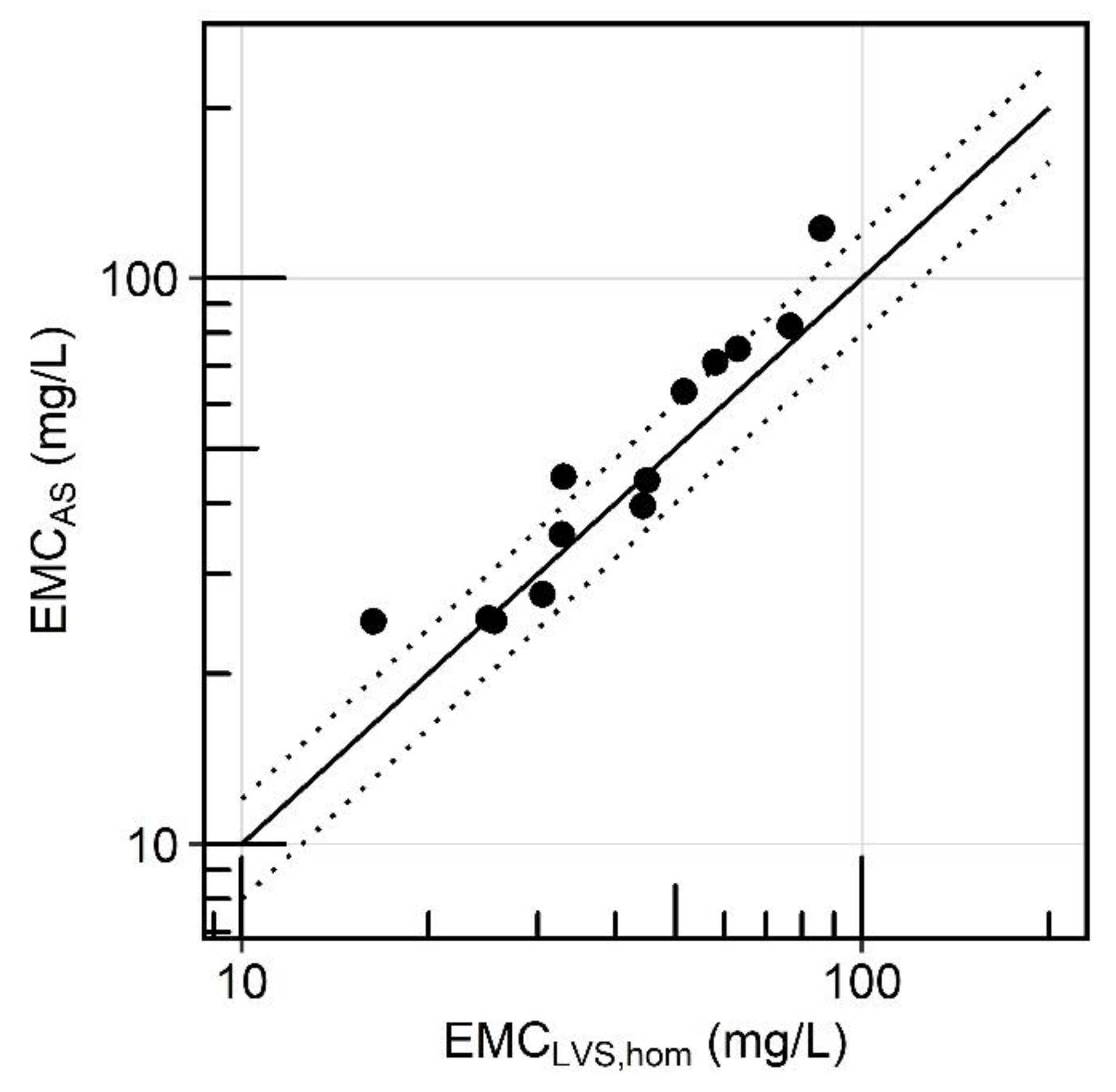
Additionally, for other events, good agreement between both sampling techniques was found (Figure 6). Most EMCAS were higher than the corresponding EMCLVS,hom, but the deviation of EMCAS from EMCLVS,hom was within a range of ±20% for most samples, even though the sampling was not harmonized, e.g., by using synchronized volume-proportional subsampling or synchronized termination of sampling. Moreover, for several events, the share of total event volume represented in the composite samples or pollutographs was different (Table 2). For three events, a deviation >20% was found. On 20 August 2019 at SES02, the LVS sampled a significantly higher share of the overflow volume, while the concentration level was particularly low (<30 mg/L). On 4 October 2019 at SES02, the LVS sampled an additional overflow peak on the following day. However, on 27 July 2019 at SES02, similar periods were covered by both AS and LVS. The differences in EMC may be due to different discrete subsampling times, lower representativeness of small volume AS subsamples (150–200 mL) compared with LVS subsamples (8–10 L), or other uncertainties in sampling and laboratory methods. Due to these influences, it cannot be conclusively determined whether the differences between EMCAS and EMCLVS,hom were systematic.
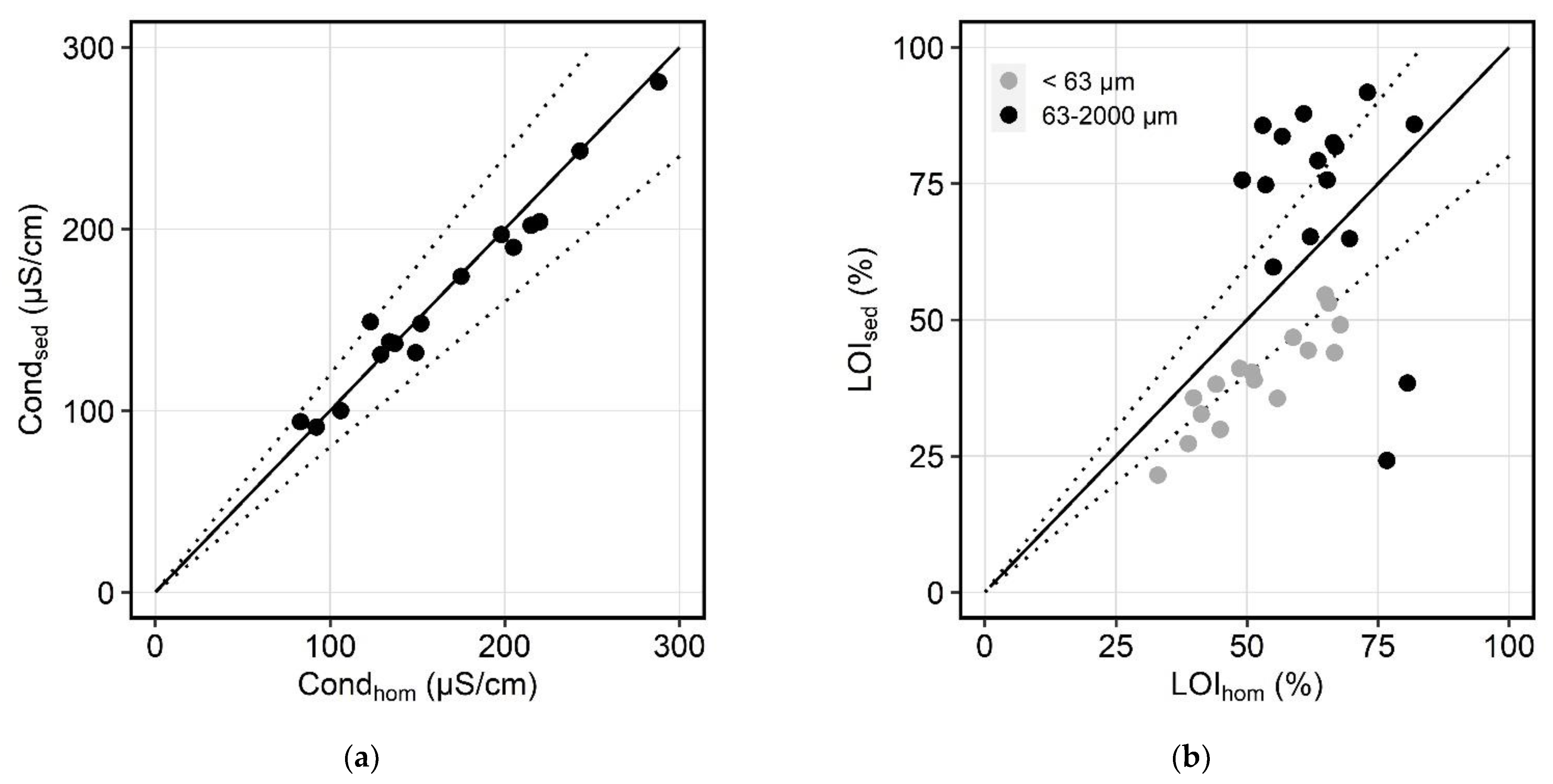
Generally, ideal representative EMC require volume-proportionally distributed subsamples from as large a part of the event as possible, with a temporal resolution adapted to concentration dynamics. Uncertainties in flow measurement may affect sampling intervals (in case of volume-proportional sampling) and the calculation of the EMC (in case of time-proportional sampling), especially if flow is derived from a function based on water level measurements. The representativeness of the EMC may be evaluated if reliable continuous TSS surrogate measurements are available, e.g., turbidity or UV-VIS online measurements [43]. However, due to fluctuations of particle composition, the relationship of TSS and surrogate measurements can rarely be assumed to be constant throughout an event. In this study, the accordance of both methods indicates that an acceptable quantification was achieved. Good agreement was also found for conductivity, COD, TP, and TNb (Figure S6).
3.3. Differences between Homogenized and Sedimented LVS Samples
LVS subsampling methods were compared for 5 inlet and 11 overflow samples (Table 2, Tables S3 and S4). EMCLVS from homogenized and sedimented samples showed acceptable agreement, but more variable differences for individual samples (Figure 7). Possible reasons for these differences are discussed in the following subsections.
3.3.1. Subsampling Bias
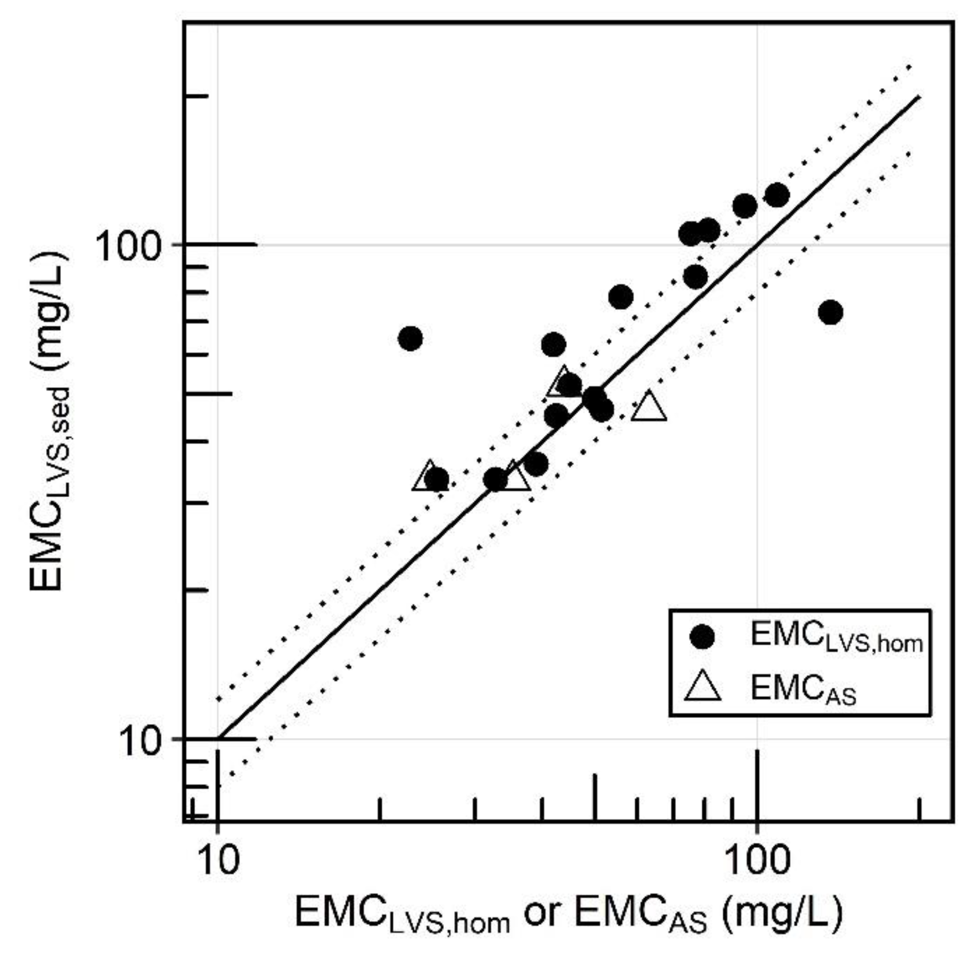
On average, EMCLVS,sed tended to be slightly higher than EMCLVS,hom, notably for concentrations >50 mg/L. This could indicate that LVS homogenization and subsampling was not sufficiently representative. The potential bias introduced by improper subsampling is known from comparisons of TSS and suspended sediment concentrations (SSC) results [44,45,46,47]. According to American standard methods, TSS are determined by filtration of a subsample, while SSC are determined from the entire sample volume [7]. If the PSD of a sample includes sand-sized particles, subsampling will likely be less representative and tend to underestimate the solids concentration [44,45]. The SSC method was demonstrated to representatively quantify EMC compared with whole-storm samples from parking lot runoff collected in a 15,000 L sample basin [48]. In this context, sedimented LVS samples might be more comparable with SSC analytical procedures. Given that the results from homogenized samples were generally confirmed by AS, this would mean that both AS and homogenized LVS could possibly underestimate TSS-EMC.
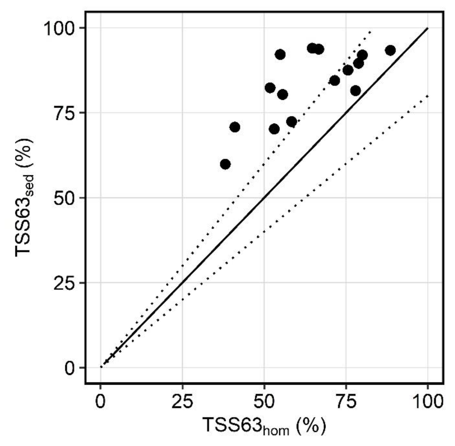
3.3.2. Size Fractionation at 63 µm
The results of the size fractionation to quantify TSS63 do not necessarily indicate bias from sand-sized particles. Instead, the percentage of TSS63 was higher in sedimented samples (Figure 8). On average, TSS63 amounted to 81% and 84% in sedimented inlet and overflow samples, respectively. In homogenized samples, TSS63 were only 63% and 68%, and showed higher variability than in sedimented samples. In order to correctly evaluate these differences, it is important to consider the mass of the solids analyzed in each method. Results from sedimented LVS samples were based on a median dry mass of 17.3 g (3.3–71.1 g). This is a factor 103 higher than the median mass analyzed in homogenized LVS samples. Only 12.2 mg (5.0–20.6 mg) was quantified after filtration of 200 mL (100–500 mL). Similar values can be obtained for the analyses of individual AS samples by filtration, i.e., 12.0 mg (1.1–35.3 mg). Therefore, if reliable size fractionation is required, sedimented samples should be preferred. These are also suitable for complete sieving analyses, as conducted by Kemper et al. [24] or Baum et al. [23].
3.3.3. Differences in Sample Processing
Differences between the results obtained for homogenized and sedimented samples are also likely affected by the sampling procedures. Both agitation during homogenization and settling before collection of the sedimented samples will alter the original in situ PSD of a sample by agglomeration of particles or disintegration of agglomerates [49]. These are effects that must be taken into account in any sampling system but could have different impacts in the two approaches. Li et al. [50] reported particle size in highway runoff samples to increase with storage time due to naturally occurring coagulation or flocculation. Contrarily, in this study, the sedimented samples taken 1–3 days after the homogenized sample showed systematically higher content of particles <63 µm. Therefore, the difference must be mainly due to other reasons, e.g., more representative sample mass and differences in analytics. This finding needs to be further explored in future research.
Another factor that could alter the sample during settling is mineralization of organic matter. Grotehusmann et al. [21] conducted 30-day stability tests of LVS samples of street runoff at 20 °C. They found a significant increase in dissolved organic carbon concentrations and conductivity in the supernatant water, indicating hydrolysis of organic matter into faster degradable dissolved organic substrates but no measurable effect on the LOI. In this study, conductivity was not affected by the settling period, but the LOI differed between homogenized and sedimented samples (Figure 9). Sedimented samples contained clay and silt particles <63 µm with systematically lower LOI and sand particles (63–2000 µm) with higher LOI than homogenized samples. This is likely not an effect of the settling period but bias introduced by limited homogenization of the water column in the tank.
3.3.4. Differences in Analytics
In addition to sampling, laboratory procedures may affect the results (Figure 4). Subsampling of homogenized samples for filtration was conducted by the shake-and-pour method. Regarding total concentrations, the laboratory homogenization was verified by comparing the sum of TSS63 and TSS >63 µm with the total TSS analyzed in a second subsample. The latter was within 82–116% (mean 100%) of the former, confirming successful homogenization. The sedimented samples were completely subjected to sieving facilitated by flushing with tap water. These two procedures may result in different levels of agglomerate disintegration. Welker et al. [51] propose to use mechanical dispersion by stirrers or blenders to obtain reproducible disintegration, while accepting potential alteration of PSD. This approach was applied by Baum et al. [23] on LVS-sedimented samples. However, it remains questionable whether it is possible to reproduce the original PSD from the moment of sample collection [49]. Moreover, it may be more important to establish reproducible methods with as few processing steps as possible. The method-related inaccuracies may be acceptable in practice.
After sieving, homogenized samples were filtered (0.6 µm), while sedimented samples were decanted and dried. Therefore, the latter also include particles < 0.6 µm, colloids, and salts dissolved in the remaining 1–1.5 L of water after decanting. Based on the conductivity measurements, the dissolved solids of each sedimented sample were estimated assuming 1 μS/cm to correspond to 0.65 mg/L. This ratio was selected from a range commonly used for natural water [52], as no data were available for CSOs. Since the relationship of dissolved solids to conductivity is influenced by wastewater composition, this should only be considered a rough estimate. The amount of dissolved solids determined in this way accounted for only a small part of the solids concentration, i.e., 0.2–5.6% (mean 1.6%).
3.4. Characterization of Solids in CSOs
3.4.1. Concentration Levels Lower than Previously Reported
Regarding sedimented LVS samples as the most representative basis, median TSS-EMC measured at the overflow of CSO facilities were 62.8 mg/L (33.5–126 mg/L). This concentration level was confirmed by 168 homogenized LVS samples collected from 12 CSOs (including the CSOs in this evaluation), with a median of 53 mg/L [53], and by other recent studies [24,54]. However, it is considerably lower than the median of 175 mg/L in a Central European CSO reported by Brombach et al. [55] based on studies from the 1970s to the 1990s. Similar TSS reductions were reported for stormwater runoff in the United States [56] and Southeastern Australia [57] when compared with previously reported studies. Francey et al. [57] suggested reduced atmospheric pollution and refined monitoring procedures as potential reasons. Our results show that a reduced concentration level must be considered for CSOs in Bavaria too.
3.4.2. Particle Size and Organic Matter Content
The solids found in CSO were dominantly clay and silt-sized particles. The median TSS63 content of LVS sediments was 84%. This corresponded well to results from other CSO in Germany [20,24]. A similar share of clay and silt-sized particles was also reported from detailed PSD analyses by laser diffraction of CSO in Italy, with d50 values of 22 to 35 μm [58].
While the TSS63 were mainly mineral particles, the fraction > 63 µm had a high organic matter content with a median LOI of 75%. The average LOI of the total samples was 45% (27–66%), indicating the potential of CSO to impact dissolved oxygen concentrations in receiving waters.
3.4.3. Pollutant Loading
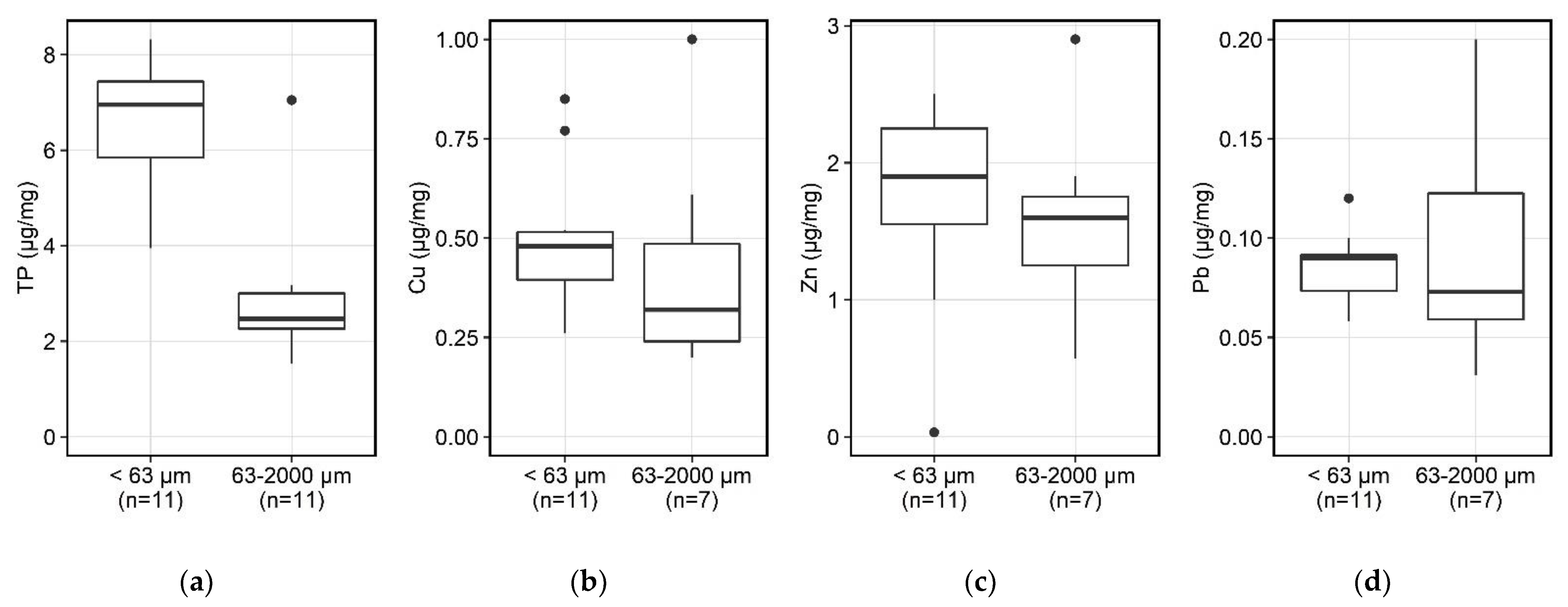
The loading of the solids with total phosphorus (TP), copper, lead, and zinc is shown in Figure 10. The results were very close to the findings by Kemper et al. [24]. Metal loading in both fractions was slightly higher than total particulate metal concentrations reported for CSO in France [2]. The magnitude of metal loading was also comparable with results of a 1997 highway runoff study [34], except for reduced lead concentrations due to the phase-out of leaded gasoline [59] and to a recent study of treated stormwater runoff [23].
There was a tendency to higher pollutant loading of TSS63 when compared with solids > 63 µm, which can be attributed to the higher specific surface area of the smaller particles. However, the difference between both fractions was significant for TP only (Mann–Whitney U Test, p < 0.001). In addition to the specific surface area, there are other parameters influencing metal adsorption, such as organic carbon content, effective cation exchange capacity, and clay-forming minerals content [36]. Kemper et al. [24] suggest that the pronounced difference for TP is due to higher content of iron oxides in the fine fractions that have a high sorption potential.
To compare the results with selected homogenized samples that were analyzed for the total metal content, particle-bound metal concentrations in the total sample were calculated (Figure S7). These concentrations are not directly comparable. Lead is mainly transported in particulate form, but zinc and copper also have relevant dissolved fractions [23,59]. Still, good agreement was found for most samples.
4. Conclusions
Generally, representative sampling in sewer systems requires a temporal resolution adapted to the concentration dynamics and the flexibility to sample widely varying event volumes and durations as completely as possible. In this regard, LVS are an efficient composite sampling technique. They come with specific advantages compared with conventional autosamplers. Whenever the research objective does not require pollutograph data but representative mean concentrations, the LVS methodology is strategically superior to standard AS due to its flexibility in capturing varying event volumes and due to lower analytical costs.
EMC derived from homogenized LVS samples and AS pollutographs of the same events were comparable even though the sampling was not synchronized. Considering the high inherent variability of the investigated sewer systems, the influence of the sampling technique can be considered negligible. TSS-EMC derived from homogenized and sedimented samples of the same LVS were also comparable. However, differing TSS63 content and loss on ignition suggested that results were impacted by the method of subsampling from LVS or laboratory procedures. Sedimented LVS samples may contain solids masses in the range of 1–1000 g, depending on the media sampled, and are therefore considered to improve the robustness and quality of particle analyses compared with conventional filtration approaches.
In general, the required sample amounts (in terms of volume or mass) and the sampling strategy are closely linked to the particular research question. The use of sedimented LVS samples is recommended for a reliable quantification of TSS loads, e.g., for the assessment of removal efficiencies of stormwater treatment facilities and for particle analyses, e.g., particle size distribution, organic matter content, or pollutant loading. Homogenized LVS samples are suitable for the quantification of pollutant EMC, long-term average concentrations, or for general screenings.
LVS are increasingly used for the monitoring of sewer systems and surface waters and are continuously being further developed. Our findings are considered important to the comparison of monitoring results of different sampling systems. Further development of LVS should also include further investigation of the observed differences between homogenized and sedimented LVS samples, e.g., regarding the quality of homogenization and the stability of samples during sedimentation in LVS.
The results obtained from LVS monitoring indicate that a lower average TSS concentration level than previously reported must be considered for CSOs in Bavaria. TSS63 were confirmed as the dominant size fraction at the inlet and overflow of centralized CSO facilities.
Supplementary Materials
The following are available online at https://www.mdpi.com/article/10.3390/w13202831/s1, Figure S1: Sketch of CSO facility SED06 with sampling points, Figure S2: Sketch of CSO facility SED02 with sampling points, Figure S3: Sketch of CSO facility SED05 with sampling point, Figure S4: Sketch of CSO facility FFR02 with sampling point, Figure S5: Sketch of CSO facility SES02 with sampling point, Figure S6: Scatterplots of EMC derived from homogenized LVS samples (EMCLVS,hom) and autosampler pollutographs (EMCAS), Figure S7: Scatterplots of EMC derived from homogenized LVS samples (EMCLVS,hom) and sedimented LVS samples (EMCLVS,sed), Table S1: Analytical methods used for water samples, Table S2: Analytical methods used for sediment samples, Table S3: Summary of analytical results of homogenized LVS samples, Table S4: Summary of analytical results of sedimented LVS samples, Table S5: Summary of analytical results of individual autosampler samples, Table S6: Summary of analytical results of autosampler EMC.
Author Contributions
Conceptualization, J.P.N. and S.F.; methodology, J.P.N. and S.F.; investigation, J.P.N.; data curation, J.P.N.; writing—original draft preparation, J.P.N.; writing—review and editing, S.F.; visualization, J.P.N.; supervision, S.F.; project administration, J.P.N. and S.F.; funding acquisition, S.F. Both authors have read and agreed to the published version of the manuscript.
Funding
This research was funded by the Bavarian State Ministry of the Environment and Consumer Protection. We acknowledge support by the KIT Publication Fund of the Karlsruhe Institute of Technology.
Institutional Review Board Statement
Not applicable.
Informed Consent Statement
Not applicable.
Data Availability Statement
The data presented in this study are available on request from the corresponding author with the permission of the Bavarian Environment Agency. The data are not publicly available as they contain confidential operational data of the CSO facilities.
Acknowledgments
We would like to thank the operators of the CSO facilities for their excellent support during the sampling campaign. We would also like to thank our partners, the Bavarian Environment Agency (Bayerisches Landesamt für Umwelt) and DVGW-Technologiezentrum Wasser (TZW) for the good cooperation. Further thanks go to Katharina Allion for her comments on an earlier draft of the manuscript.
Conflicts of Interest
The authors declare no conflict of interest. The funders had no role in the design of the study; in the collection, analyses, or interpretation of data; in the writing of the manuscript; or in the decision to publish the results.
References
- Launay, M.; Dittmer, U.; Steinmetz, H. Organic micropollutants discharged by combined sewer overflows-Characterisation of pollutant sources and stormwater-related processes. Water Res. 2016, 104, 82–92. [Google Scholar] [CrossRef] [PubMed]
- Becouze-Lareure, C.; Dembélé, A.; Coquery, M.; Cren-Olivé, C.; Bertrand-Krajewski, J.-L. Assessment of 34 dissolved and particulate organic and metallic micropollutants discharged at the outlet of two contrasted urban catchments. Sci. Total Environ. 2019, 651, 1810–1818. [Google Scholar] [CrossRef] [PubMed]
- Fuchs, S.; Scherer, U.; Wander, R.; Behrendt, H.; Venohr, M.; Opitz, D.; Hillenbrand, T.; Marscheider-Weidemann, F.; Götz, T. Calculation of Emissions into Rivers in Germany Using the MONERIS Model: Nutrients, Heavy Metals and Polycyclic Aromatic Hydrocarbons; Texte 46/2010; Umweltbundesamt (UBA): Dessau-Roßlau, Germany, 2010.
- Paijens, C.; Bressy, A.; Frère, B.; Tedoldi, D.; Mailler, R.; Rocher, V.; Neveu, P.; Moilleron, R. Urban pathways of biocides towards surface waters during dry and wet weathers: Assessment at the Paris conurbation scale. J. Hazard. Mater. 2021, 402, 123765. [Google Scholar] [CrossRef]
- Wicke, D.; Matzinger, A.; Sonnenberg, H.; Caradot, N.; Schubert, R.-L.; Dick, R.; Heinzmann, B.; Dünnbier, U.; von Seggern, D.; Rouault, P. Micropollutants in Urban Stormwater Runoff of Different Land Uses. Water 2021, 13, 1312. [Google Scholar] [CrossRef]
- Bilotta, G.S.; Brazier, R.E. Understanding the influence of suspended solids on water quality and aquatic biota. Water Res. 2008, 42, 2849–2861. [Google Scholar] [CrossRef]
- Pitt, R.E.; Clark, S.; Eppakayala, V.K.; Sileshi, R. Don’t Throw the Baby Out with the Bathwater-Sample Collection and Processing Issues Associated with Particulate Solids in Stormwater. J. Water Manag. Modeling 2017, 25, C416. [Google Scholar] [CrossRef] [Green Version]
- Todeschini, S.; Papiri, S.; Ciaponi, C. Placement Strategies and Cumulative Effects of Wet-weather Control Practices for Intermunicipal Sewerage Systems. Water Resour. Manag. 2018, 32, 2885–2900. [Google Scholar] [CrossRef]
- Kim, J.-Y.; Sansalone, J.J. Event-based size distributions of particulate matter transported during urban rainfall-runoff events. Water Res. 2008, 42, 2756–2768. [Google Scholar] [CrossRef]
- Fuchs, S.; Lambert, B.; Grotehusmann, D. Neue Aspekte in der Behandlung von Siedlungsabflüssen. Umweltwiss. Schadst. Forsch. 2010, 22, 661–667. [Google Scholar] [CrossRef] [Green Version]
- Selbig, W.; Fienen, M.; Horwatich, J.; Bannerman, R. The Effect of Particle Size Distribution on the Design of Urban Stormwater Control Measures. Water 2016, 8, 17. [Google Scholar] [CrossRef] [Green Version]
- Lee, H.; Swamikannu, X.; Radulescu, D.; Kim, S.; Stenstrom, M.K. Design of stormwater monitoring programs. Water Res. 2007, 41, 4186–4196. [Google Scholar] [CrossRef]
- Madoux-Humery, A.-S.; Dorner, S.; Sauvé, S.; Aboulfadl, K.; Galarneau, M.; Servais, P.; Prévost, M. Temporal variability of combined sewer overflow contaminants: Evaluation of wastewater micropollutants as tracers of fecal contamination. Water Res. 2013, 47, 4370–4382. [Google Scholar] [CrossRef]
- Barco, J.; Papiri, S.; Stenstrom, M.K. First flush in a combined sewer system. Chemosphere 2008, 71, 827–833. [Google Scholar] [CrossRef]
- Lee, J.H.; Bang, K.W.; Ketchum, L.H.; Choe, J.S.; Yu, M.J. First flush analysis of urban storm runoff. Sci. Total Environ. 2002, 293, 163–175. [Google Scholar] [CrossRef]
- Wittmer, I.K.; Bader, H.-P.; Scheidegger, R.; Singer, H.; Luck, A.; Hanke, I.; Carlsson, C.; Stamm, C. Significance of urban and agricultural land use for biocide and pesticide dynamics in surface waters. Water Res. 2010, 44, 2850–2862. [Google Scholar] [CrossRef]
- Ma, J.-S.; Kang, J.-H.; Kayhanian, M.; Stenstrom, M.K. Sampling Issues in Urban Runoff Monitoring Programs: Composite versus Grab. J. Environ. Eng. 2009, 135, 118–127. [Google Scholar] [CrossRef]
- McCarthy, D.T.; Zhang, K.; Westerlund, C.; Viklander, M.; Bertrand-Krajewski, J.-L.; Fletcher, T.D.; Deletic, A. Assessment of sampling strategies for estimation of site mean concentrations of stormwater pollutants. Water Res. 2018, 129, 297–304. [Google Scholar] [CrossRef] [PubMed]
- McCarthy, D.; Harmel, D. Quality assurance/quality control in stormwater sampling. In Quality Assurance & Quality Control of Environmental Field Sampling; Zhang, C., Mueller, J.F., Mortimer, M.R., Eds.; Future Science Ltd.: London, UK, 2014; pp. 98–127. [Google Scholar]
- Fuchs, S.; Mayer, I.; Haller, B.; Roth, H. Lamella settlers for storm water treatment-performance and design recommendations. Water Sci. Technol. 2014, 69, 278–285. [Google Scholar] [CrossRef]
- Grotehusmann, D.; Lambert, B.; Fuchs, S.; Graf, J. Konzentrationen und Frachten Organischer Schadstoffe im Straßenabfluss: Schlussbericht zum BASt Forschungsvorhaben FE-Nr; 05.152/2008/GRB; Bundesanstalt für Straßenwesen (BASt): Bergisch Gladbach, Germany, 2014.
- Eyckmanns-Wolters, R.; Fuchs, S.; Maus, C.; Sommer, M.; Voßwinkel, N.; Mohn, R.; Uhl, M. Reduktion des Feststoffeintrags durch Niederschlagswassereinleitungen (REFENI). Phase 1: Projektbericht. 2013. Available online: http://isww.iwg.kit.edu/medien/Abschlussbericht_ReduktionFeststoffeintragPhase1.pdf (accessed on 7 September 2019).
- Baum, P.; Kuch, B.; Dittmer, U. Adsorption of Metals to Particles in Urban Stormwater Runoff—Does Size Really Matter? Water 2021, 13, 309. [Google Scholar] [CrossRef]
- Kemper, M.; Eyckmanns-Wolters, R.; Fuchs, S.; Ebbert, S.; Maus, C.; Uhl, M.; Weiß, G.; Nichler, T.; Engelberg, M.; Gillar, M.; et al. Analyse der Leistungsfähigkeit von Regenüberlaufbecken und Überwachung durch Online Messtechnik. Abschlussbericht. 2015. Available online: https://isww.iwg.kit.edu/download/2015_12_16_Schlussbericht_Monitoring.pdf (accessed on 7 September 2021).
- Nickel, J.P.; Fuchs, S. Micropollutant emissions from combined sewer overflows. Water Sci. Technol. 2019, 80, 2179–2190. [Google Scholar] [CrossRef]
- Fuchs, S.; Kaiser, M.; Reid, L.; Toshovski, S.; Nickel, J.P.; Gabriel, O.; Clara, M.; Hochedlinger, G.; Trautvetter, H.; Hepp, G.; et al. Grenzüberschreitende Betrachtung des Inn-Salzach-Einzugsgebietes als Grundlage für ein transnationales Gewässermanagement. Unpublished Report. 2019. [Google Scholar]
- Fuchs, S.; Rothvoß, S.; Toshovski, S. Ubiquitäre Schadstoffe–Eintragsinventare, Umweltverhalten und Eintragsmodellierung; Texte 52/2018; Umweltbundesamt (UBA): Dessau-Roßlau, Germany, 2018.
- Wagner, A. Event-Based Measurement and Mean Annual Flux Assessment of Suspended Sediment in Meso Scale Catchments; Dissertation; Institut für Wasser und Gewässerentwicklung, Fachbereich Siedlungswasserwirtschaft und Wassergütewirtschaft: Karlsruhe, Germany, 2020. [Google Scholar]
- Nickel, J.P.; Fuchs, S. Qualitative Untersuchung von Mischwasserentlastungen in Bayern: Schlussbericht; Karlsruher Institut für Technologie (KIT): Karlsruhe, Germany, 2020. [Google Scholar]
- DWA-A 102-2/BWK-A 3-2. Arbeitsblatt DWA-A 102-2/BWK-A 3-2 Grundsätze zur Bewirtschaftung und Behandlung von Regenwetterabflüssen zur Einleitung in Oberflächengewässer: Teil 2: Emissionsbezogene Bewertungen und Regelungen; Deutsche Vereinigung für Wasserwirtschaft, Abwasser und Abfall: Hennef, Germany, 2020; ISBN 9783968620466. [Google Scholar]
- Droppo, I.G.; Irvine, K.N.; Jaskot, C. Flocculation/aggregation of cohesive sediments in the urban continuum: Implications for stormwater management. Environ. Technol. 2002, 23, 27–41. [Google Scholar] [CrossRef]
- Zhao, H.; Jiang, Q.; Xie, W.; Li, X.; Yin, C. Role of urban surface roughness in road-deposited sediment build-up and wash-off. J. Hydrol. 2018, 560, 75–85. [Google Scholar] [CrossRef]
- Fuchs, S.; Kemper, M.; Nickel, J.P. Feststoffe in der Regenwasserbehandlung. In 52. Essener Tagung für Wasserwirtschaft vom 20.-22. März 2019 in Aachen, Wasser und Gesundheit; Pinnekamp, J., Ed.; Gesellschaft zur Förderung der Siedlungswasserwirtschaft an der RWTH Aachen e.V.: Aachen, Germany, 2019; ISBN 978-3-938996-56-0. [Google Scholar]
- Sansalone, J.J.; Buchberger, S.G. Characterization of solid and metal element distributions in urban highway stormwater. Water Sci. Technol. 1997, 36, 155–160. [Google Scholar] [CrossRef]
- Vaze, J.; Chiew, F.H.S. Nutrient Loads Associated with Different Sediment Sizes in Urban Stormwater and Surface Pollutants. J. Environ. Eng. 2004, 130, 391–396. [Google Scholar] [CrossRef]
- Gunawardana, C.; Egodawatta, P.; Goonetilleke, A. Role of particle size and composition in metal adsorption by solids deposited on urban road surfaces. Environ. Pollut. 2014, 184, 44–53. [Google Scholar] [CrossRef] [Green Version]
- Boogaard, F.C.; van de Ven, F.; Langeveld, J.G.; Kluck, J.; van de Giesen, N. Removal efficiency of storm water treatment techniques: Standardized full scale laboratory testing. Urban Water J. 2016, 14, 255–262. [Google Scholar] [CrossRef]
- Michelbach, S.; Wöhrle, C. Settleable Solids from Combined Sewers: Settling, Stormwater Treatment, and Sedimentation Rates in Rivers. Water Sci. Technol. 1994, 29, 95–102. [Google Scholar] [CrossRef]
- Fugate, D.; Chant, B. Aggregate settling velocity of combined sewage overflow. Mar. Pollut. Bull. 2006, 52, 427–432. [Google Scholar] [CrossRef]
- DIN EN 872. Wasserbeschaffenheit-Bestimmung Suspendierter Stoffe-Verfahren Durch Abtrennung Mittels Glasfaserfilter; Deutsche Fassung EN 872:2005; Deutsches Institut für Normung e. V.: Berlin, Germany, 2005. [Google Scholar]
- Baum, P.; Benisch, J.; Blumensaat, F.; Dierschke, M.; Dittmer, U.; Gelhardt, L.; Gruber, G.; Grüner, S.; Heinz, E.; Hofer, T.; et al. AFS63-Harmonisierungsbedarf und Empfehlungen für die labortechnische Bestimmung des neuen Parameters. In Regenwasser in Urbanen Räumen. Aqua Urbanica Trifft Regenwassertage, Landau in der Pfalz, 18.-19.06.2018; Schmitt, T.G., Ed.; Technische Universität Kaiserslautern: Kaiserslautern, Germany, 2018; pp. 153–168. ISBN 978-3-95974-086-9. [Google Scholar]
- Sprenger, J.; Tondera, K.; Linnemann, V. Determining fine suspended solids in combined sewer systems: Consequences for laboratory analysis. In Proceedings of the 9th International Conference on Planning and Technologies for Sustainable Management of Water in the City (NOVATECH 2016), Lyon, France, 28 June–1 July 2016. [Google Scholar]
- Sandoval, S.; Bertrand-Krajewski, J.-L.; Caradot, N.; Hofer, T.; Gruber, G. Performance and uncertainties of TSS stormwater sampling strategies from online time series. Water Sci. Technol. 2018, 78, 1407–1416. [Google Scholar] [CrossRef] [PubMed] [Green Version]
- Selbig, W.R.; Bannerman, R.T. Ratios of Total Suspended Solids to Suspended Sediment Concentrations by Particle Size. J. Environ. Eng. 2011, 137, 1075–1081. [Google Scholar] [CrossRef]
- Gray, J.R.; Glysson, G.D.; Turcios, L.M.; Schwarz, G.E. Comparability of Suspended-Sediment Concentration and Total Suspended Solids Data; U.S. Department of the Interior: Reston, VA, USA, 2000.
- Galloway, J.M.; Evans, D.A.; Green, W.R. Comparability of Suspended-Sediment Concentration and Total Suspended-Solids Data for Two Sites on the L’Anguille River, Arkansas, 2001 to 2003: Scientific Investigations Report 2005-5193; U.S. Geological Survey: Reston, VA, USA, 2005.
- Clark, S.E.; Siu, C.Y.S. Measuring Solids Concentration in Stormwater Runoff: Comparison of Analytical Methods. Environ. Sci. Technol. 2008, 42, 511–516. [Google Scholar] [CrossRef]
- Roseen, R.M.; Ballestero, T.P.; Fowler, G.D.; Guo, Q.; Houle, J. Sediment Monitoring Bias by Automatic Sampler in Comparison with Large Volume Sampling for Parking Lot Runoff. J. Irrig. Drain Eng. 2011, 137, 251–257. [Google Scholar] [CrossRef] [Green Version]
- Phillips, J.M.; Walling, D.E. An assessment of the effects of sample collection, storage and resuspension on the representativeness of measurements of the effective particle size distribution of fluvial suspended sediment. Water Res. 1995, 29, 2498–2508. [Google Scholar] [CrossRef]
- Li, Y.; Lau, S.-L.; Kayhanian, M.; Stenstrom, M.K. Particle Size Distribution in Highway Runoff. J. Environ. Eng. 2005, 131, 1267–1276. [Google Scholar] [CrossRef]
- Welker, A.; Dierschke, M.; Gelhardt, L. Methodische Untersuchungen zur Bestimmung von AFS63 (Feine Abfiltrierbare Stoffe) in Verkehrsflächenabflüssen. Wasser Abwasser 2019, 4, 79–88. [Google Scholar]
- Rusydi, A.F. Correlation between conductivity and total dissolved solid in various type of water: A review. IOP Conf. Ser.Earth Environ. Sci. 2018, 118, 12019. [Google Scholar] [CrossRef]
- Nickel, J.P.; Sacher, F.; Fuchs, S. Up-to-date monitoring data of wastewater and stormwater quality in Germany. Water Res. 2021, 202, 117452. [Google Scholar] [CrossRef]
- Clara, M.; Gruber, G.; Humer, F.; Hofer, T.; Kretschmer, F.; Ertl, T. SCHTURM-Spurenstoffemissionen aus Siedlungsgebieten und von Verkehrsflächen; Austrian Ministry of Agriculture, Forestry, Environment and Water Management: Vienna, Austria, 2014.
- Brombach, H.; Weiss, G.; Fuchs, S. A new database on urban runoff pollution: Comparison of separate and combined sewer systems. Water Sci. Technol. 2005, 51, 119–128. [Google Scholar] [CrossRef] [PubMed]
- Smullen, J.T.; Shallcross, A.L.; Cave, K.A. Updating the U.S. nationwide urban runoff quality data base. Water Sci. Technol. 1999, 39, 9–16. [Google Scholar] [CrossRef]
- Francey, M.; Fletcher, T.D.; Deletic, A.; Duncan, H. New Insights into the Quality of Urban Storm Water in South Eastern Australia. J. Environ. Eng. 2010, 136, 381–390. [Google Scholar] [CrossRef]
- Piro, P.; Carbone, M.; Garofalo, G.; Sansalone, J. Size Distribution of Wet Weather and Dry Weather Particulate Matter Entrained in Combined Flows from an Urbanizing Sewershed. Water Air Soil Pollut. 2010, 206, 83–94. [Google Scholar] [CrossRef]
- Huber, M.; Welker, A.; Helmreich, B. Critical review of heavy metal pollution of traffic area runoff: Occurrence, influencing factors, and partitioning. Sci. Total Environ. 2016, 541, 895–919. [Google Scholar] [CrossRef] [PubMed]
Figure 1.
General setup of the large-volume sampler.

Figure 2.
Methods for subsampling from large-volume composite samples.

Figure 3.
Photographs of the large-volume samplers and subsampling procedures used in this study.

Figure 4.
Analytical steps for measuring the concentration of total suspended solids < 63 µm (TSS63).
Figure 4.
Analytical steps for measuring the concentration of total suspended solids < 63 µm (TSS63).

Figure 5.
Evolution of the TSS event mean concentrations (EMCAS) derived from the autosamplers pollutograph (CAS) during a combined sewer overflow (CSO) event compared to the EMC derived from the large-volume samplers (EMCLVS,hom).
Figure 5.
Evolution of the TSS event mean concentrations (EMCAS) derived from the autosamplers pollutograph (CAS) during a combined sewer overflow (CSO) event compared to the EMC derived from the large-volume samplers (EMCLVS,hom).

Figure 6.
Scatterplot of TSS event mean concentrations derived from homogenized large-volume samplers samples (EMCLVS,hom) and autosamplers pollutographs (EMCAS). Dotted lines show 20% deviation.
Figure 6.
Scatterplot of TSS event mean concentrations derived from homogenized large-volume samplers samples (EMCLVS,hom) and autosamplers pollutographs (EMCAS). Dotted lines show 20% deviation.

Figure 7.
Scatterplot of TSS event mean concentrations derived from homogenized (EMCLVS,hom) and sedimented (EMCLVS,sed) large-volume samplers samples. Triangles show the EMC derived from autosamplers (EMCAS) pollutographs of the same events compared with sedimented samples. Dotted lines show 20% deviation.

Figure 8.
Scatterplot of the percentage of TSS <63 µm measured in homogenized (TSS63hom) and sedimented (TSS63sed) large-volume samplers samples. Dotted lines show 20% deviation.
Figure 8.
Scatterplot of the percentage of TSS <63 µm measured in homogenized (TSS63hom) and sedimented (TSS63sed) large-volume samplers samples. Dotted lines show 20% deviation.

Figure 9.
Scatterplots of conductivity (Cond) (a) and loss on ignition (LOI) (b) measured in homogenized (hom) and sedimented (sed) large-volume samplers samples. Dotted lines show 20% deviation.
Figure 9.
Scatterplots of conductivity (Cond) (a) and loss on ignition (LOI) (b) measured in homogenized (hom) and sedimented (sed) large-volume samplers samples. Dotted lines show 20% deviation.

Figure 10.
Pollutant loading of sedimented LVS samples collected from combined sewer overflows: (a) Total phosphorus (TP), (b) Copper (Cu), (c) Zinc (Zn), (d) Lead (Pb).
Figure 10.
Pollutant loading of sedimented LVS samples collected from combined sewer overflows: (a) Total phosphorus (TP), (b) Copper (Cu), (c) Zinc (Zn), (d) Lead (Pb).


Table 1.
Properties of the samplers used in the sampling campaign.
| Property | Large-Volume Sampler | Autosampler |
|---|---|---|
| Sampling strategy | Volume-proportional | Time-proportional |
| Sampling interval | 40–350 m3 | 3 min |
| Subsample volume | 8–10 L | 150–200 mL |
| Sample containers | Stainless steel, 1000 L | PE, 12–24 × 1 L |
| Samples per container | 10–100 | 5–6 |
| Pumping system | Peristaltic | Vacuum |
| Pump capacity | 1090 L∙h−1 | No data available |
| Pumping speed | ~0.62 m∙s−1 | >0.5 m∙s−1 |
| Suction height | Max. 8 m | Max. 8 m |
| Max. particle size | 5 mm | No data available |
| Suction hose | PVC, Ø 25 mm | PVC, Ø 12–16 mm |
| Active cooling | No | Yes |
Table 2.
Events sampled with large-volume samplers (LVS) or autosamplers (AS) at the inlet or overflow of combined sewer overflow (CSO) facilities.
Table 2.
Events sampled with large-volume samplers (LVS) or autosamplers (AS) at the inlet or overflow of combined sewer overflow (CSO) facilities.
| CSO Facility | Date (MM-dd-yyyy) | Total Overflow Duration (h) | Total Overflow Volume (m3) | Share of Total Volume Represented in the Composite Sample or Pollutograph (%) * | |||
|---|---|---|---|---|---|---|---|
| LVS Overflow | LVS Inlet | AS Overflow | AS Inlet | ||||
| SED06 | 09-04-2018 | 1.5 | 4504 | 100 I,II | - | - | - |
| SED06 | 09-23-2018 | 2.6 | 7215 | 100 I,II | 100 I,II | - | - |
| SED06 | 05-20-2019 | 24.2 | 43,880 | - | 100 I,II | - | - |
| SED06 | 06-22-2019 | 4.1 | 10,167 | 100 I,II | - | - | - |
| SED06 | 07-01-2019 | 1.4 | 6282 | 100 I,II | - | - | - |
| SED06 | 07-28-2019 | 6.3 | 15,173 | 100 I,II | - | - | - |
| SED02 | 12-02-2018 | 8.8 | 2807 | 100 I,II | 100 I,II | - | - |
| SED02 | 05-11-2019 | 5.1 | 1657 | 100 I,II | 100 I,II | 76 | 82 |
| SED02 | 10-01-2019 | 8.9 | 2721 | 100 I,II | 100 I,II | 46 | 53 |
| SED05 | 10-09-2019 | 7.5 | 2481 | 100 I | - | 33 | - |
| FFR02 | 09-23-2018 | 4.8 | 8474 | 99 I,II | - | - | - |
| FFR02 | 12-02-2018 | 4.7 | 4306 | 100 I,II | - | - | - |
| FFR02 | 10-05-2019 | 1.7 | 2054 | 100 I,II | - | - | - |
| SES02 | 05-20-2019 | 46.0 | 71,054 | 11 I | - | 7 | - |
| SES02 | 05-28-2019 | 12.4 | 9353 | 81 I | - | 51 | - |
| SES02 | 07-01-2019 | 5.2 | 5827 | 100 I | - | 100 | - |
| SES02 | 07-27-2019 | 12.8 | 20,777 | 36 I | - | 40 | - |
| SES02 | 08-02-2019 | 4.1 | 6227 | 100 I | - | 100 | - |
| SES02 | 08-20-2019 | 11.8 | 9890 | 77 I | - | 43 | - |
| SES02 | 10-04-2019 | 11.8 | 9015 | 86 I | - | 40 | - |
| SES02 | 10-30-2019 | 12.7 | 8255 | 94 I | - | 53 | - |
* Refers to CSO volume for overflow samples and to the sum of storage and CSO volume for inlet samples. I Homogenized sample collected. II Sedimented sample collected. - Not sampled.
Publisher’s Note: MDPI stays neutral with regard to jurisdictional claims in published maps and institutional affiliations. |
© 2021 by the authors. Licensee MDPI, Basel, Switzerland. This article is an open access article distributed under the terms and conditions of the Creative Commons Attribution (CC BY) license (https://creativecommons.org/licenses/by/4.0/).
Share and Cite
MDPI and ACS Style
Nickel, J.P.; Fuchs, S. Large-Volume Samplers for Efficient Composite Sampling and Particle Characterization in Sewer Systems. Water 2021, 13, 2831. https://doi.org/10.3390/w13202831
AMA Style
Nickel JP, Fuchs S. Large-Volume Samplers for Efficient Composite Sampling and Particle Characterization in Sewer Systems. Water. 2021; 13(20):2831. https://doi.org/10.3390/w13202831
Chicago/Turabian StyleNickel, Jan Philip, and Stephan Fuchs. 2021. "Large-Volume Samplers for Efficient Composite Sampling and Particle Characterization in Sewer Systems" Water 13, no. 20: 2831. https://doi.org/10.3390/w13202831
Note that from the first issue of 2016, this journal uses article numbers instead of page numbers. See further details here.