
Can Simple Machine Learning Tools Extend and Improve Temperature-Based Methods to Infer Streambed Flux?
by
 ,
,
Mohammad A. Moghaddam
1, 
Ty P. A. Ferré
1,* ,
,
Xingyuan Chen
2,
Kewei Chen
2,
Xuehang Song
2 and
Glenn Hammond
3 1
Department of Hydrology and Atmospheric Sciences, University of Arizona, Tucson, AZ 85721, USA
2
Pacific Northwest National Laboratory, Richland, WA 99354, USA
3
Sandia National Laboratory, Albuquerque, NM 87123, USA
*
Author to whom correspondence should be addressed.
Water 2021, 13(20), 2837; https://doi.org/10.3390/w13202837
Submission received: 20 July 2021
/
Revised: 25 September 2021
/
Accepted: 2 October 2021
/
Published: 12 October 2021
(This article belongs to the Section Hydrogeology)
Abstract
:Temperature-based methods have been developed to infer 1D vertical exchange flux between a stream and the subsurface. Current analyses rely on fitting physically based analytical and numerical models to temperature time series measured at multiple depths to infer daily average flux. These methods have seen wide use in hydrologic science despite strong simplifying assumptions including a lack of consideration of model structural error or the impacts of multidimensional flow or the impacts of transient streambed hydraulic properties. We performed a “perfect-model experiment” investigation to examine whether regression trees, with and without gradient boosting, can extract sufficient information from model-generated subsurface temperature time series, with and without added measurement error, to infer the corresponding exchange flux time series at the streambed surface. Using model-generated, synthetic data allowed us to assess the basic limitations to the use of machine learning; further examination of real data is only warranted if the method can be shown to perform well under these ideal conditions. We also examined whether the inherent feature importance analyses of tree-based machine learning methods can be used to optimize monitoring networks for exchange flux inference.
1. Introduction
There is a long-standing interest in developing methods to quantify surface-water–ground-water exchange flux to better understand water and solute exchange across the sediment-water interface. Some studies require that multidimensional stream/aquifer flux be described with high spatial and temporal resolution, perhaps including consideration of time-varying streambed hydraulic properties [1,2,3]. Other applications only require an accurate estimate of the local vertical water flux [4,5,6]. Hydrologic studies exist along this spectrum, giving rise to a need for a range of methods that provide flux estimates with different resolutions and requiring different levels of measurement support.
To quantify water flux, several methods have been developed, including seepage meters, differential-discharge measurements, shallow piezometers, tracer experiments, and temperature-tracer measurements [7,8,9,10]. Due to the underlying assumptions, the labor intensiveness, the tempo-spatial resolution, and uncertainty costs, each of these methods have limitations in most cases, which are described in detail in [11]. However, there is a particular interest in applying thermal-based methods to measure flux. These methods involve the interpretation of temperature time series, collected in the subsurface, to estimate 1D vertical exchange flux across the streambed [12,13,14,15,16,17,18,19]. These methods are particularly well-suited to measurements under field conditions over large areas where the practical advantages of self-contained logging temperature sensors make them clearly superior to pressure-based methods. In general, temperature-based methods have been based on inferring conductive–convective heat transport from time series of temperature at multiple depths to estimate water flux. To date, temperature-based methods to infer 1D vertical exchange flux across a streambed have relied on fitting analytical or numerical models of coupled flow and heat transport to subsurface temperature time series. Initial methods fit an analytical solution describing the subsurface response to a sinusoidally varying surface temperature forcing [12,13]. Later approaches have used numerical models to infer infiltration from temperature time series measured in the surface water and in the subsurface [14]. Despite the simplifications that underly these 1D temperature methods, they have made major contributions to the understanding of reach-to-watershed scale hydrology. However, several previous researchers have recognized that uncertainty in the sediment thermal parameters can translate to uncertainty in flux estimates [10,17]. Moreover, these approaches generally require relatively long (hours to days) time series for calibration. Furthermore, the flux estimates have been limited to relatively low temporal resolution—hours to months—because the available data do not support unique inversion of the water flux boundary condition at a time resolution similar to the data collection frequency. Finally, to date, no published methods have considered estimating water flux under conditions of temporally varying, temperature-dependent hydraulic conductivity using those methods.
With advances in sensor technology and wireless communication, automated groundwater monitoring systems provide us the opportunity to collect groundwater data with high temporal resolution. With the aforementioned advancement in data collection as well as storage and computation power, data-driven methods, such as machine learning (ML) and deep learning (DL), are transforming many scientific disciplines, specifically in water resources management and hydrogeology. In general, the power of ML and DL methods lies in their ability to learn more complex functions while providing enhanced generalization capabilities. Further, recent studies [20,21,22,23] have shown the computational benefits of ML/DL models as surrogates of physics-based models, relying on intensive numerical simulation.
In this study, we performed an initial investigation of the possibility of replacing these physics-based models with simple machine learning algorithms to infer the exchange flux with higher temporal resolution and whether these same tools can inform optimal sensor network design. Our objective was to examine the potential uses of simple machine learning (ML) techniques to augment numerical model-based analyses of streambed infiltration/exfiltration. Specifically, we aimed to determine whether simple ML methods, trained on a numerical model, could provide near-real-time flux estimations based on five-minute resolution subsurface pressure and temperature time series. Further, we examined whether the ML tools could be used to identify a reduced observation network, ideally comprised of only temperature sensors, that contained all information necessary to infer the surface/subsurface flux. If successful, ML tools could be paired with relatively few sensors to extend monitoring of water flux across the ground surface at low cost after an initial, more intensive calibration period.
2. Materials and Methods
This study represents an initial feasibility study of using machine learning (ML) to infer 1D streambed flux based on subsurface temperature time series. To provide an ideal, testable basis for this examination, we performed a “perfect-model experiment,” making use of model-generated temperature and pressure measurements with corresponding, model-generated groundwater/surface water exchange fluxes. For this, a highly resolved numerical model of water flow and heat transport produced exchange flux time series at the streambed as well as temperature and pressure time series at multiple depths. The numerical model’s configuration is described in detail in [24]. The numerical model outputs were used as inputs for the ML analyses. The exchange fluxes were the forecast targets, and the temperature and water pressure time series at multiple depths were the features. In particular, the input features (derived from the temperature and pressure observations) were temperature/pressure, time-delayed temperature/pressure, and temperature/pressure gradients in space and time. These inputs and targets are referred to as flux time series and subsurface pressure and temperature time series. Both the temperature and pressure measurements were subjected to varying levels of measurement noise to assess the impact of measurement uncertainty on flux estimation.
The results of a “perfect-model experiment” are only strictly meaningful in pointing out limitations to a method. A more complete test of the promise of ML methods for inferring flux from subsurface temperature time series should consider model structural error and, ideally, field observations collected with high temporal and spatial resolution. However, a perfect-model experiment offers a near-ideal initial test of a method. In the context of this study, if model-generated error-free observations’ data cannot support the prediction of exchange fluxes that are generated by the same model, then we can conclude that it is unlikely that the proposed ML method and data will be successful in practice. Further, we can examine the impact of observation error on the method’s performance. If the results are promising with added error, then it is worthwhile to conduct further investigations that examine the influence of model structural uncertainty, the impact of multidimensional hyporheic flow, and time-varying streambed sediment properties, among other complicating factors. However, it should be noted that none of these complications have limited the use of current temperature-based exchange flux estimation methods even though they use physically based models that do not consider them.
2.1. Generation of Noise-Free Observations with a Numerical Flow and Heat Transport Model
This study is part of a series of investigations aimed at determining water flux between the Columbia River and its underlying aquifer. As a part of these investigations, a 3D PFLOTRAN [25] model was constructed to simulate fully-coupled nonisothermal flow and heat transport in the subsurface. PFLOTRAN is a parallel multiphase flow simulator implemented in object-oriented FORTRAN that uses an integral volume finite difference approach with the nonlinearities in the discretized equation resolved thorough Newton Raphson iteration. This 3D model was constructed to simulate flow and heat transport near the Columbia River at the Hanford 300 A area in Washington [24]. The model domain is 400 m × 400 m × 20 m, including three layers with different hydraulic and thermal properties (alluvium, Hanford, and Ringold formations). The spatial resolution of the uppermost, alluvium layer was 0.5 m × 2 m × 0.1 m to capture the flow and temperature dynamics in the shallow subsurface.
The objective of this study was to test the use of ML methods to infer 1D vertical flow. Therefore, a 1D model simulating flow and heat transport was built to generate the subsurface temperature and pressure time series at multiple depths and the corresponding exchange fluxes at the streambed. The 1D vertical model is 2 m in vertical extent with a spatial resolution of 0.01 m; this high spatial resolution was necessary to provide accurate temperatures and pressures at the observation depths. The boundary conditions applied to the 1D model were extracted from the 3D model, thereby transferring as much of the information from the 3D system as possible. The top and bottom boundaries of the 1D model were of Dirichlet type for both flow and heat transport. The 1D model was homogeneous, with a permeability equal to that of the alluvium layer, 3.86 × 10⁻¹¹ m2. The simulation period was 1 January 2016–30 June 2017 (1.5 years) with temperature, pressure, and streambed flux generated every 5 min.
Both the 1D and 3D models accounted for the temperature dependence of the viscosity following:
where μw is water dynamic viscosity in micropoise (μP), T is temperature in degrees Kelvin (K), p is pressure in bars, and psat is saturation pressure in bars corresponding to temperature T [26].
2.2. Model-Generated Time Series Used for Machine Learning Analyses
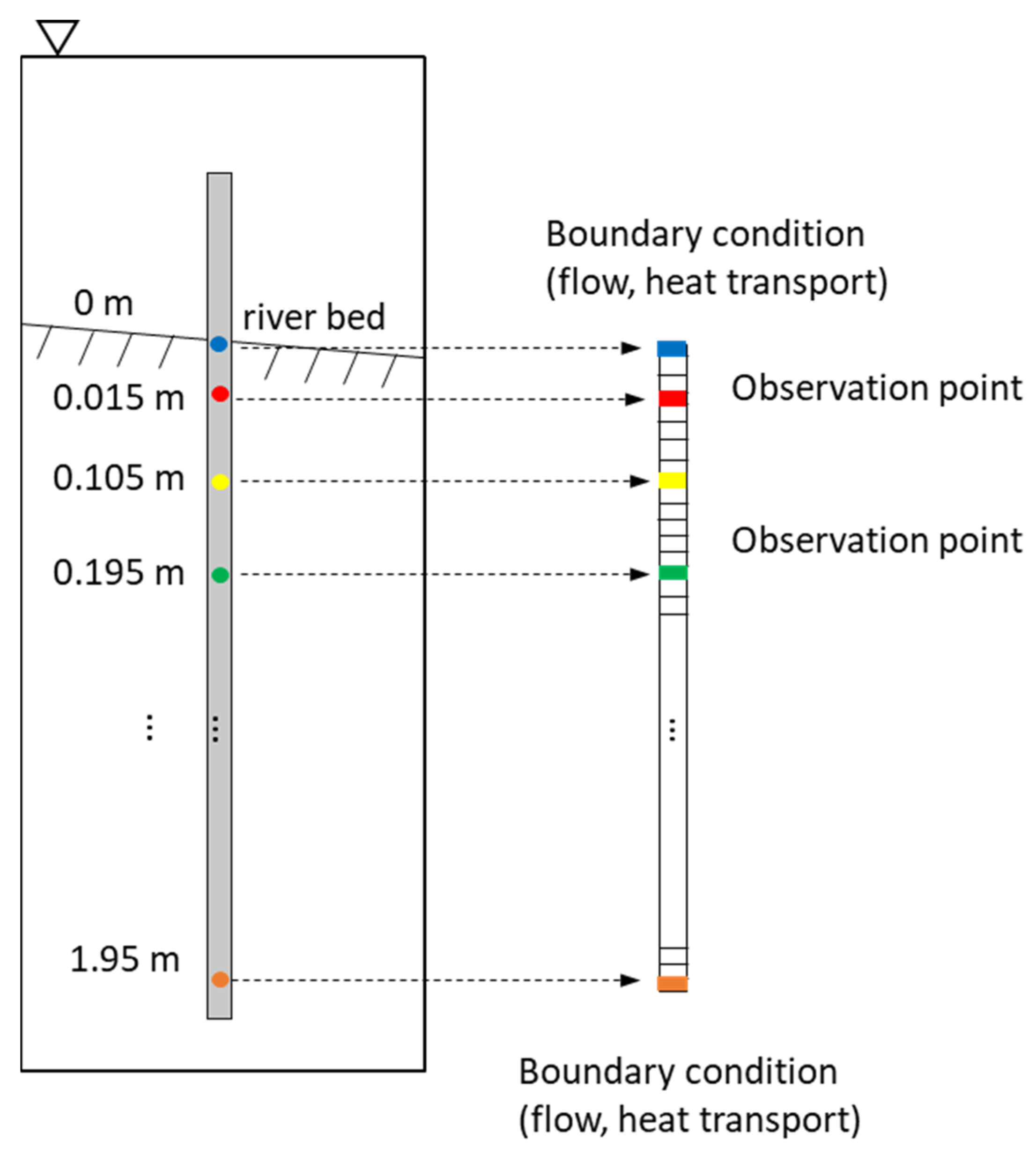
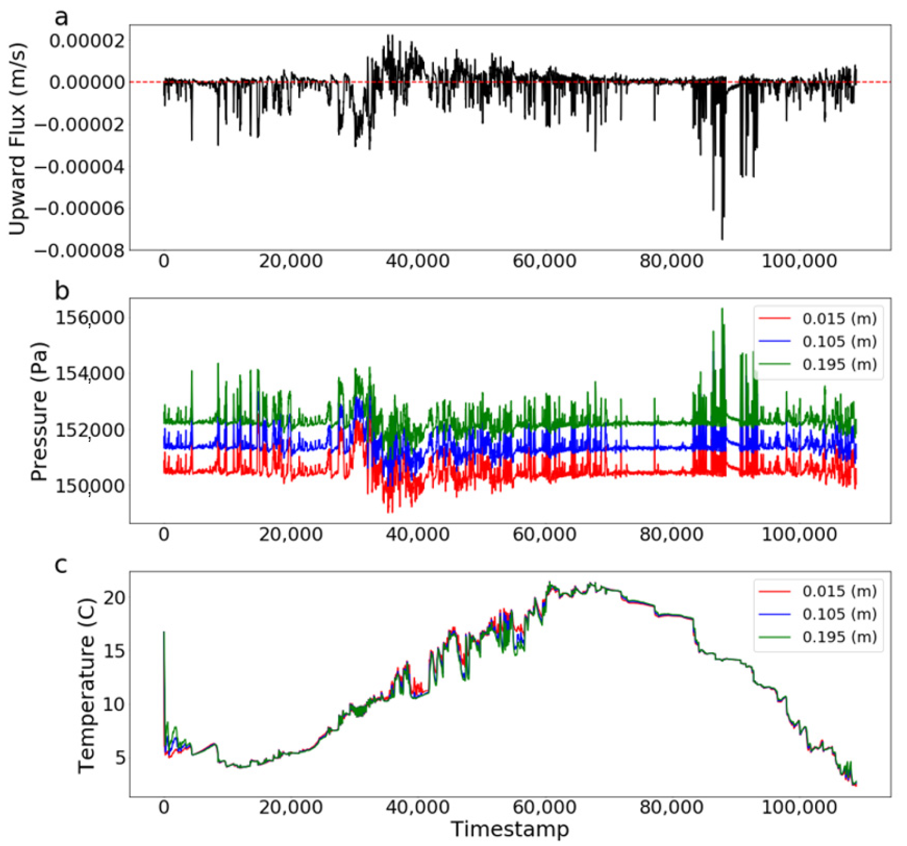
The high-resolution 1D vertical flow and heat transport PFLOTRAN model generated pressure and temperature at 200 depths with a 0.01 m spacing between 0.005 and 1.995 m depth below the riverbed. We considered a subset of these measurement depths to represent a plausible monitoring network with sensors at depths of 0.015, 0.105, and 0.195 m. These depths represent a measurement immediately below the stream bed and two sensors placed at approximately 10 cm separation (Figure 1). It should be reiterated that this initial study was a perfect-model experiment. Therefore, the numerical model results were used, with and without added error, to represent sensor responses that could be collected in the field. The resulting time series of streambed flux (Figure 2A), subsurface pressure (Figure 2B), and subsurface temperature (Figure 2C) were interpreted using simple, tree-based ML methods. The nature of flow in the modeled system resulted in predominantly low streambed fluxes with more instances of downward flux than upward. The maximum downward flux (shown throughout as negative upward flux) was greater than the maximum upward flux (Figure 2A).
2.3. Training and Testing the ML Tools
We considered two machine learning methods: regression trees and gradient boosting, referred to as RT and GB, respectively. The basic structure of these methods is presented below for the benefit of readers who are not familiar with them.
2.4. Implementation of Regression Tree Analyses
RT techniques consider paired values of targets (here, streambed exchange flux) and features (in this case, subsurface temperature and/or pressure observations and/or their spatial gradients, between any two observation depths or temporal gradients or between any two observation times at a common depth). All of the available data were divided into training and testing subsets. The RT considers the training data, searching through the features and dividing the targets based on the value of each feature. In this investigation, two subsets at each split were formed. The feature and the associated threshold value of that feature that result in two subsets with the smallest sample-weighted total variance was identified, and the set was divided into two subsets (Figure 3). This procedure was repeated for each subset until a user-selected number of splits or until the reduction in variance due to splitting failed to meet a user-defined limit. The sequence of feature/threshold values was identified based on the training data, and the performance of the trained RT was based on its ability to predict the targets in the testing set based on the corresponding testing features. (See further discussion of the specific training/testing performed for this study below.) One limitation of RT methods is that they are “greedy,” meaning that the feature and threshold is identified at each node sequentially, without consideration of the overall optimal set of features and thresholds. For this reason, RT is not guaranteed to be optimally efficient. Rather, it is seen as a relatively simple, rapid ML approach that results in a tree structure that is relatively easy to interpret.
The performance of the RT depends on the choice of several user-defined values (hyperparameters). A process of hyperparameter tuning allows for the performance to be improved. However, to accomplish this, the training data set has to be further divided into a training set and a validation set. The training set is used first, then the validation set is used for hyperparameter tuning. Finally, the as-yet-unused testing set can be used to assess the performance of the trained RT. For our implementation, the hyperparameters were: number of levels of the RT, the minimum reduction in variability required, and the minimum population of a subset needed to justify branching at a node. The tree-based methods used in this study were tuned using cross validation [27]; the parameter values are reported in the Appendix A in Table A1.
A strength of RT is its ease of interpretation. Consider the illustrative example shown in Figure 3. Temperatures measured at ten depths, T(1) through T(10), were considered to form a tree with only two children formed at each node and two levels of nodes. The initial set, including all the training fluxes, was composed of 3486 samples with a mean value of 0.666 m/s; the MSE between all the flux values and the mean was 0.032. The RT process identified the shallowest temperature observation, T(1), with a threshold of 14.37 °C as the first feature for classification. This divides the fluxes into two groups with mean values of 0.749 and 0.583 and sample sizes of 745 and 2741, respectively. The sample-weighted MSE can be calculated for each split by multiplying the MSE of that set by the number of samples in the set after splitting normalized by the total number of samples. In the illustrative example, the sample-weighted MSE after splitting was 0.022. The left branch identified T(1), again, as the best criterion with a threshold of 5.12 °C, but this did not meet the minimum required improvement in MSE to continue, so this branch was terminated without splitting. The right branch identified T(10) with a threshold of 14.51 °C. This split met the variance reduction criterion, so the samples were divided into two subsets with mean values of 0.890 and 0.612 m/s. To apply the RT at some time, t, in the testing set, only T(1) and T(10) would be considered. If these values were T(1) = 15.0 and T(10) = 13.2, then the binary classification at each branch leads to the central box with a mean value of 0.890 m/s. This value of predicted flux at that time would be compared to the known flux at that time to assess the performance of the trained RT.
The highly simplified example shown in Figure 3 demonstrates how RT can be used for monitoring network design. That is, for this example, measurements T(2) through T(9) were not considered when applying the RT, so they could be eliminated from the measurement design with no loss of accuracy. Beyond this simple elimination approach, we can quantify the relative importance of T(1) and T(10) by examining how much each reduces the sample-weighted variability of the training set. Specifically, at each node we can quantify the population-weighted reduction in MSE as:
where ni is the number of observations in each subset after splitting, MSEi is the corresponding mean squared error of each post-split subset, np is the number of observations in the parent set (before splitting), and MSEp is the mean squared error of the parent set. These nodal importance values can be summed for each observation (e.g., for all instances of T(1)) and then normalized by the sum over all observations to define the relative contribution of each observation:
in which J is the set of all nodes considering observation j, and K is the set of all nodes. In this case, observation T(1) has an importance of 0.72, and T(10) has an importance of 0.28. In this way, many features can be considered when constructing an RT, and their contribution to the inference can be quantified easily, as an inherent part of constructing the RT. Practical considerations, such as cost or ease of installation, can then be combined with the feature importance results to select a reduced set of observations.
2.5. Implementation of Gradient Boosting Tree
RT is a conceptually accessible ML method. However, it has several well-recognized limitations [28,29]. RT can be susceptible to overfitting, especially if the input data are noisy. The sequential, “greedy” nature of RT can miss combinations of splitting rules that may lead to better classification. Additionally, because each leaf (final box on Figure 3) is represented by the mean value of its samples, the model produces discontinuous, stepped predictions, especially for trees with relatively few levels. Finally, RT expends computational effort to attempt to subdivide every node on every level, whereas it may be more efficient to expend more effort on areas where the RT is underperforming. These limitations of RTs can be mitigated to some degree by adding gradient boosting. Boosting begins by constructing a relatively weak RT (e.g., with relatively few levels). Then, a second RT is constructed to predict the prediction errors (the residuals) of the first tree. This is repeated sequentially, continually reducing the largest prediction errors [30,31,32,33,34]. The feature importance values of the sequence of RTs are combined to define the overall contribution of each feature to the RT with gradient boosting (hereafter referred to as GB). For our implementation, the hyperparameters are:
The number of weak learners, the number of levels, the learning rate, and the minimum population of a subset needed to justify branching at a node.
2.6. Training and Testing the ML Algorithms
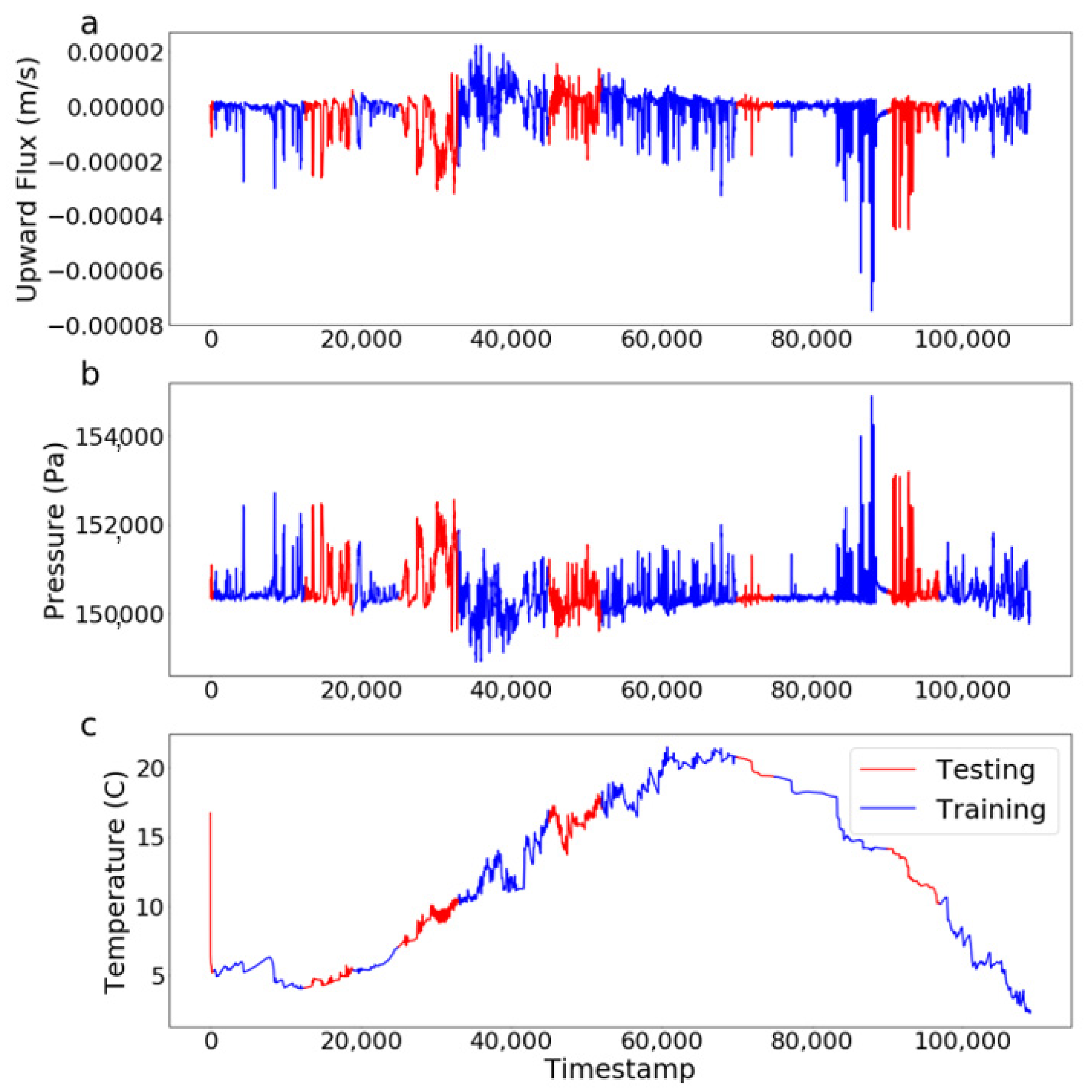
A key decision facing all ML analyses involves the definition of training and testing subsets of the data. The training sets were used to determine the features; the associated threshold values were used to segregate the data; and the testing set was used to assess its performance. Generally, the ML will only be adept at predicting conditions that are bounded by those included in the training set; that is, the training data must be representative of the full range of conditions. However, care must be taken to ensure that the testing data are independent of the training set to avoid providing unintended information to the ML. For example, if data collected every even minute was used for training and every odd minute for testing, the ML would make use of the high temporal correlation of the testing and training data. However, if the ML were applied to new data with a different distribution, it would likely underperform compared to the training results. Following general guidelines for training/testing splits [35,36], we used 70% of the data for training and the remaining 30% for testing. For this investigation, both training and testing sets must sample the full range of both temperature and flux conditions to be fully representative. Because the hydraulic conductivity depends on the temperature, and the flux depends on the hydraulic conductivity, care had to be taken to include samples from throughout the year, as the daily average temperature varied seasonally. This required that several discontinuous periods be included in the training set. Simultaneously, it was necessary to avoid having training information leak into the testing set due to temporal correlation of the training and testing observations. In particular, given that there is a diffusive element of heat transport, it is likely the temperature measurements that are close in time will be highly correlated. To avoid this effect, we instituted a buffer time of 100 min at the beginning and end of each training period; samples within these buffers were not used for testing or training. To satisfy all these requirements, we divided the 110,000 observation times into six paired training/testing periods (Figure 4) to cover all ranges of flux values during both training and testing periods. Training was performed on observations: 500–12,500, 19,000–25,000, 33,000–45,000, 52,000–70,000, 75,000–90,000, and 97,000–110,000 (shown in blue). We also used five-fold cross validation on training period to tune the model [27]. Specifically, testing was performed on the remaining observations (shown in red) with the measurements in the buffer zones not included (not visible on Figure 4).
In this study, we added zero mean Gaussian random errors with a standard deviation equal to a given percent of the variance of all measurements of a given type (e.g., all temperature measurements) collected at all depths and times. That is, the level of relative measurement error was assumed to be comparable for temperature and pressure sensors. This analysis could be repeated for different relative temperature and pressure errors if there was reason to believe that the available sensors had different error characteristics. To conform to general descriptions of measurement error, these errors are described as a signal to noise ratio (SNR). For example, if the variance of the error free observations is 100 times the applied variance of the added errors, then the SNR is reported as 100. A measurement set with an SNR of 10 would be considerably noisier than one with an SNR of 100.
As described above, tree-based ML methods can consider many possible features and identify the most informative (important) as an integral part of forming the RT. Therefore, we decided to consider the temperature and pressure time series, and we also examined whether temporal and spatial gradients of temperature and pressure were more informative than direct measurements. From a hydrologic perspective, we might expect that pressure gradients, which are directly related to vertical water flow through the hydraulic conductivity, may be more informative than a pressure measurement at a single depth. To reflect practically achievable gradient observations, spatial gradients were calculated between the sensor depths already included in the observation set; that is, the addition of gradient measures did not increase the number of subsurface sensors needed. We assumed that measurements were collected every 5 min, so the temporal gradient was calculated for a 5-min time delay. We also considered measurements made at the time of streambed flux inference and observations made before and after the time of inference. This is particularly useful for temperature measurements because it takes time for the change in surface flux to impact downward advective heat transport such that there is a noticeable affect at a sensor at depth. (Note, streambed flux estimation is rarely, if ever, made in real time. As such, there is no prohibition on using data after the time of inference.) Specifically, we considered temperature and pressure observations and their spatial and temporal gradients with delays ranging from −30 to +30 min, with a 5-min resolution, as the inputs for the models.
3. Results and Discussion
We used RT and GB to infer the exchange flux based on model-generated subsurface temperature and pressure data with and without added noise. Each method was applied to the same training/testing sets to allow for direct comparison of their performance. Analyses were performed on observation sets in the following order: temperature and pressure data at multiple depths, only temperature data at multiple depths, and collocated pressure and temperature sensors at a single depth.
3.1. Analyses of Temperature and Pressure Data at Multiple Depths
To define the optimal achievable performance for a practical observation set, we first considered all of the available data. Given that we are performing a perfect-model experiment, which has a reasonable goal of perfect prediction of streambed flux, we only described the ML performance based on cross-plots of the true and inferred streambed flux through time.
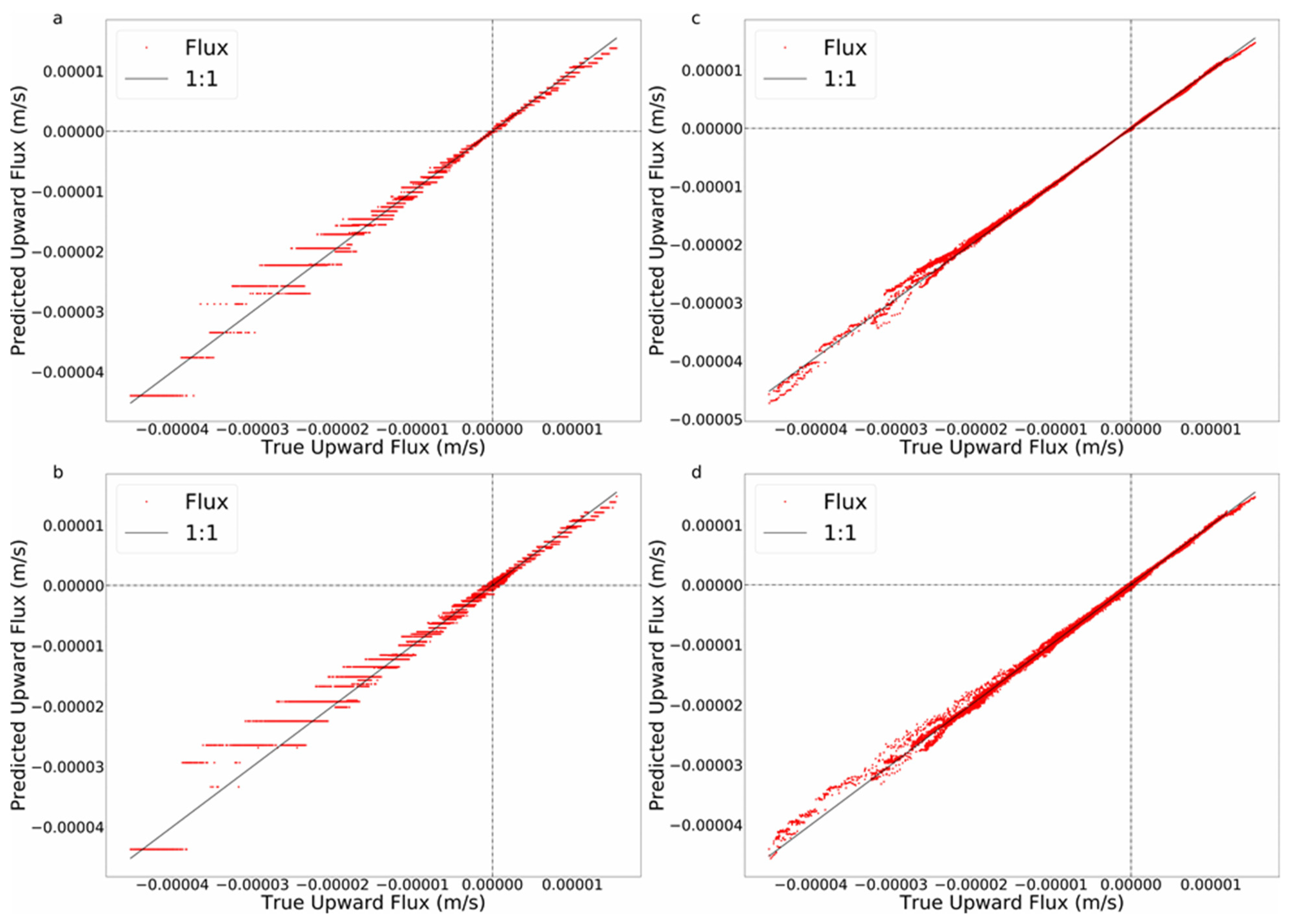
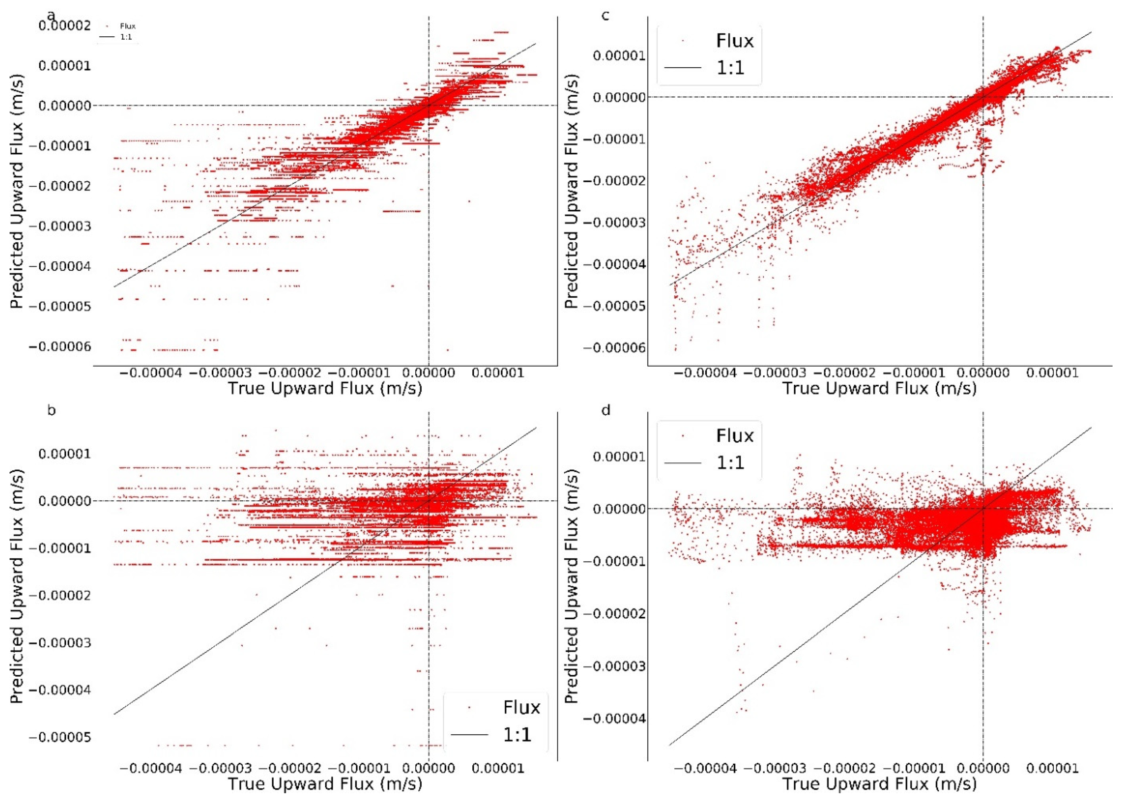
The RT was able to infer upward fluxes very accurately with no added noise (Figure 5a). Downward flux (shown as negative upward flux) was less well resolved. Specifically, both upward and downward fluxes were estimated accurately for fluxes less than approximately 0.00002 m/s; estimates of higher downward fluxes showed more error. From a physical perspective, this is surprising; temperature-based estimation based on matching a physical model relies on advective heat transport to propagate the temperature variations at the surface to the measurement locations, resulting in greater sensitivity to downward flow. Closer examination of the results shown in Figure 5 point to an explanation that offers insight into a possible limitation of this use of ML. Namely, remembering that RT produces discretized values of flux (one for each terminal leaf), the larger spacing between the flux estimates for high downward fluxes indicates that the majority of the effort of the RT was used to refine the lower upward and downward fluxes. This is likely due to the relative rarity of high downward fluxes, as seen in Figure 5a. The addition of noise with an SNR of 100 (Figure 5c) had little impact on the quality of inference of lower upward or downward fluxes. However, added noise further degraded the quality of the estimates of high downward fluxes. Adding gradient boosting greatly improved the exchange flux estimation, especially for high downward fluxes (Figure 5b). This improvement illustrates the advantage of gradient boosting techniques, which inherently concentrate on reducing the largest errors at each level of the analysis, which resulted in much more finely resolved, and accurate, flux estimations based on combined temperature and pressure data. The addition of 100 SNR measurement error had very little impact on the performance of GB when considering both pressure and temperature measurements at multiple depths.
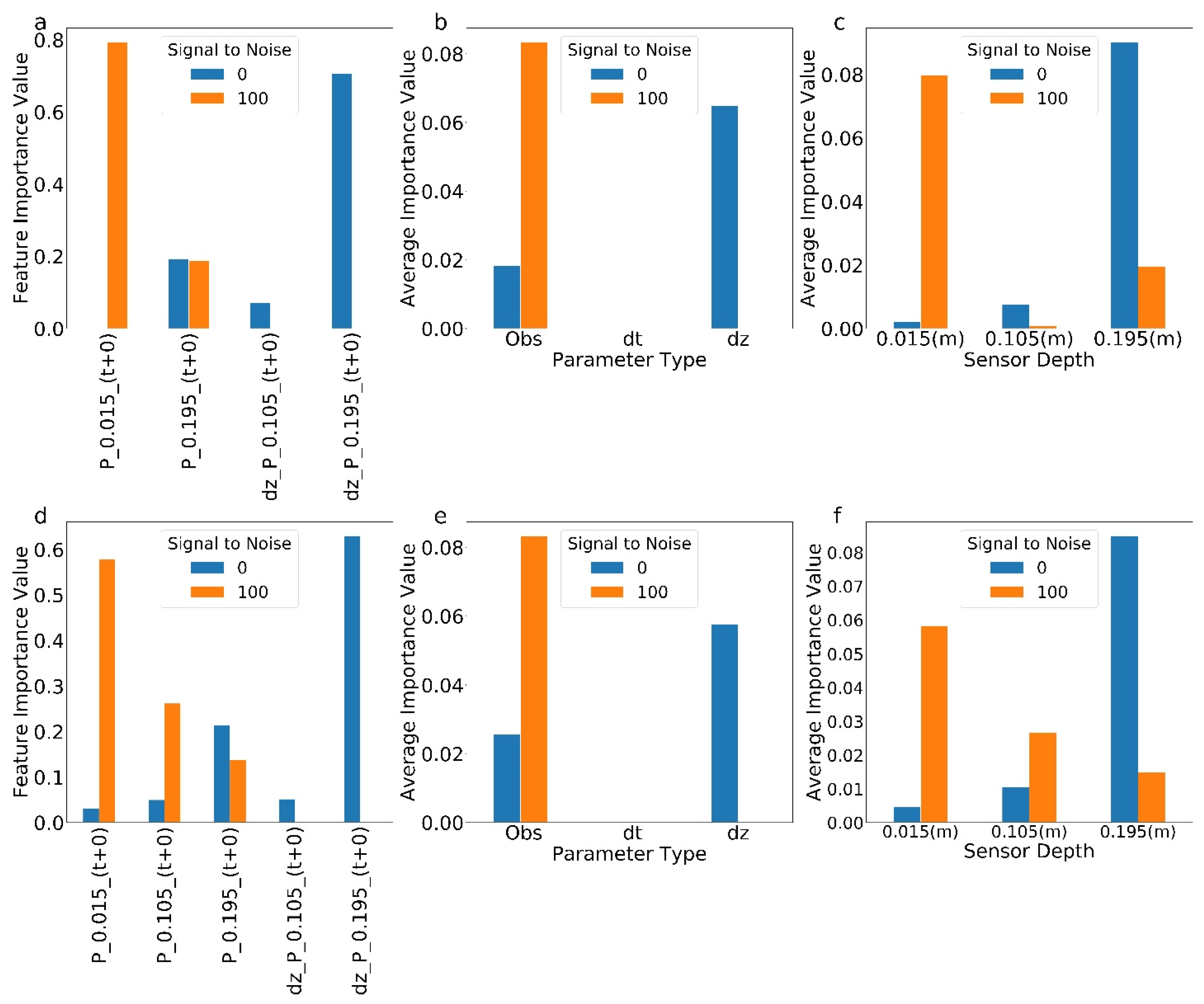
The built-in feature importance assessment of RT allows for relatively simple interpretation of the observations (types, depths, delays, or gradients) that contribute to the regression (Figure 6). RT and GB, with and without added noise, were provided with all of the data—temperature and pressure measurements: observations and temporal and spatial gradients. A specific observation was identified by its type (P = pressure, T = temperature, dz = spatial gradient, or dt = temporal gradient), its depth in meters (0.015, 0.105, or 0.195), and its time delay relative to the time of exchange flux inference (e.g., −15 = 15 min prior, +10 = 10 min after). When assessing feature importance with added noise, it was necessary to consider the feature importance over multiple error realizations. We considered 100 realizations, each with the same SNR but different specific error realizations, and averaged the results.
The clearest result is that only pressure and spatial gradients of pressure were identified as important features for RT and GB and for data with and without added noise (Figure 6a,d). This was expected given that pressure is more directly related to flux, through Darcy’s Equation, than is temperature, through heat transport and through the advection dispersion equation. In addition, all of these features were collected at the time of flux inference. This likely indicates that the pressure associated with the exchange flux propagated through the system very quickly. There are some consistent impacts of added noise for RT and GB. Specifically, without noise, both algorithms preferred spatial gradients of pressure collected at greater depth. Adding noise increased the reliance on direct measurements at shallower depths. This, again, is consistent with our expectations: with added noise, the absolute signal should be increased (shallower rather than deeper measurements), and instantaneous gradients will magnify measurement errors (observations rather than calculated gradients). The fact that these results, based only on the feature importance, agree with our expectations based on physical insights give us more confidence in the use of tree-based ML methods to identify optimal observation sets. Importantly, this approach to measurement network design does not require the computationally expensive combinatorial analyses that are common for these investigations. The design recommendations are produced automatically as part of the ML training.
3.2. Analyses of Temperature Data Only
Temperature-based methods were developed for field use because temperature sensors are more robust and less expensive than pressure sensors [14,15,16,17]. Therefore, despite the clear preference for pressure observations, we continued our examination of the possible use of temperature only. Because regression trees are greedy, and we showed that pressure observations are more important than temperature observations, we can only assess the value of temperature observations by removing the pressure data from consideration. Even considering model-generated data with no added noise (Figure 7a), there was clear degradation of the accuracy of the inferred flux when using only temperature data. The results are improved somewhat for GB (Figure 7b). However, neither was tree-based ML able to predict the surface exchange flux with high temporal resolution based on temperature observations with added measurement error with an SNR of 100 (Figure 7c,d). We also examined whether RT or GB could resolve the average flux calculated over nonoverlapping 30-min windows; yet, the results were not improved significantly (not shown).
3.3. Analyses of Pressure and Temperature Observations Collected at a Single Depth
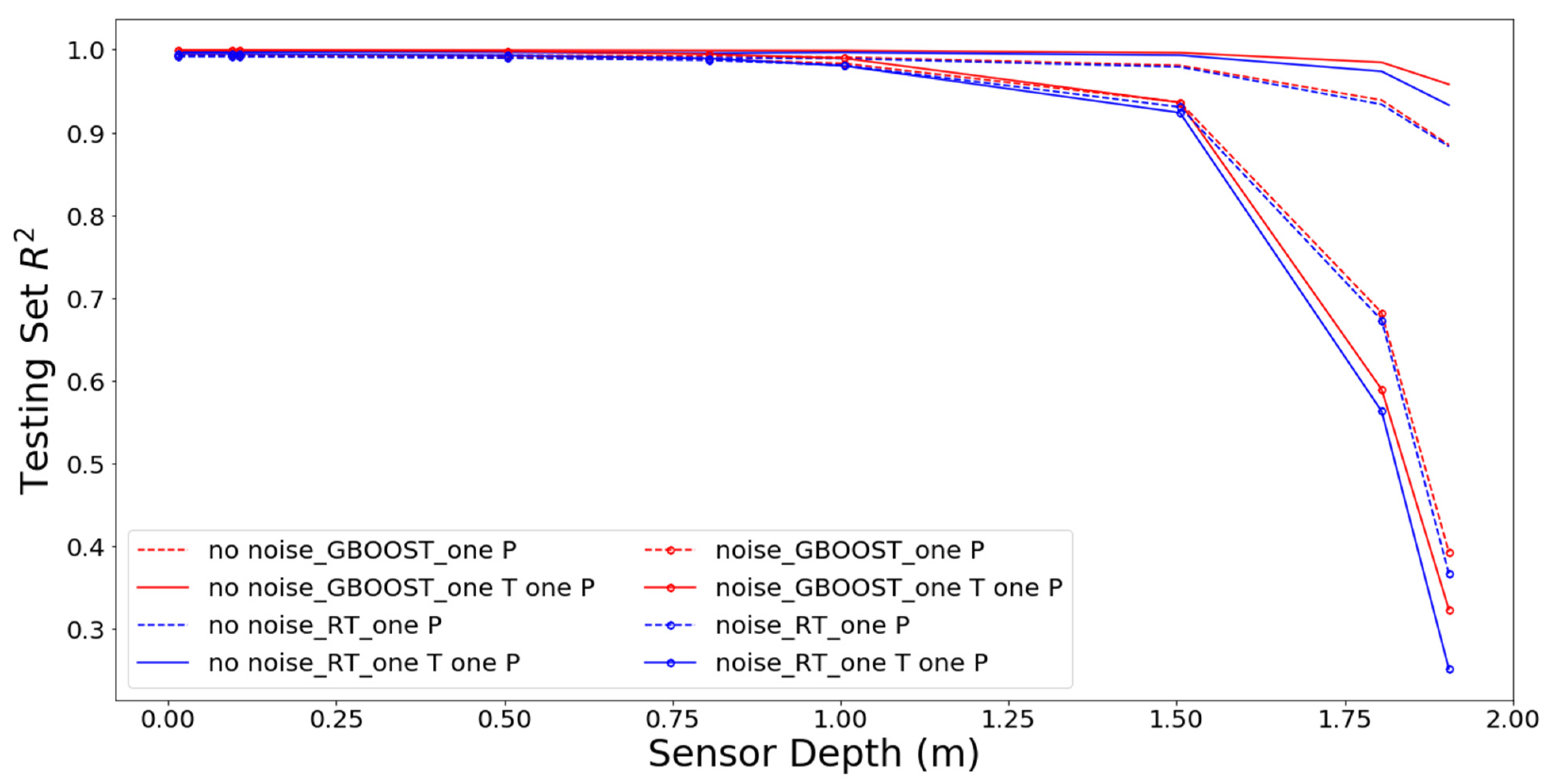
The results of our investigation show clearly that RT and GB showed a strong preference for pressure measurements as the basis for inferring surface exchange flux. The impetus for developing temperature-based methods was largely practical, based on the difficulties of using pressure sensors under field conditions. Therefore, we decided to examine whether ML methods could be used to design a compromise solution based on a single sensor that measures pressure or both pressure and temperature. The performance is shown on Figure 8 as a function of the sensor depth, the type of sensor (P or combined P and T), and whether GB is used. In all cases, GB improved the performance (red versus blue lines). The presence of measurement noise (series with symbols) dramatically decreased performance for deeper sensors but had little impact on shallower sensors. Adding temperature data (solid versus dashed lines) improved the performance when error was not considered, but it significantly degraded the performance of deep sensors with measurement error included. Of greatest practical significance, sensors placed within the shallowest 50 cm performed very well; yet, they showed relatively little improvement with the addition of GB or temperature measurements. This application demonstrates a way in which perfect-model experiments can be used to streamline the measurement network design process. In this case, if RT or GB is to be used to infer the exchange flux, there appears to be little value in collecting temperature data, and pressure data should be collected within the shallowest 50 cm of the streambed. The next step in network design would be to repeat this analysis with more advanced ML algorithms before testing the findings in the field.
4. Conclusions
We demonstrated the use of a perfect-model experiment as a first test of the possible use of regression trees (with and without gradient boosting) to infer the exchange flux between a stream and the subsurface with high temporal resolution based on subsurface pressure and temperature observations. Specifically, we used a numerical model to generate paired water pressure and temperature values through time at several depths beneath a river. We then examined whether ML can be trained to recover the times series of flux between the river and the subsurface. Such a perfect-model examination, which does not consider possible model structural errors, cannot be used to validate an approach. Rather, only two conclusions can be drawn: either that a proposed method does not work under these idealized conditions, so it is unlikely to work in the field, or, that the proposed approach meets the first test of effectiveness and is worth examining under more challenging conditions. We simultaneously conducted a value-of-information analysis to determine which observations are most valuable for inferring this flux. The results showed that pressure observations were far more informative than temperature observations. In fact, with any realistic level of added noise, RT or GB was not able to infer streambed exchange flux accurately from subsurface temperature time series alone. Analysis of flux estimation based on observations at a single, shallow depth are promising, warranting further examination. However, these results also suggest that adding temperature information has little or no value. The primary finding from this investigation was that a perfect-model experiment approach, combined with the inherent feature importance measures of RT or GB, offers an efficient initial assessment of proposed measurement network designs. This efficiency was due to the built-in feature importance analyses of these tree-based methods, which provide valuable insight into the flow of information from observations to predictions with essentially no added computational cost beyond training the ML. Clearly, a successful result from a perfect-model experiment does not validate a proposed measurement network. However, failure constitutes strong evidence that the network is not likely to be successful under less ideal conditions. Future work should extend these analyses to more sophisticated ML methods and to other hydrologic monitoring network design challenges.
Author Contributions
All authors developed the idea for this paper, accomplished the analysis and wrote the manuscript together. All authors have read and agreed to the published version of the manuscript.
Funding
This research was supported by the U.S. Department of Energy (DOE) (Washington, DC, USA), Office of Biological and Environmental Research (BER), as part of BER’s Subsurface Biogeochemical Research Program (SBR). This contribution originates from the SBR Scientific Focus Area (SFA) at the Pacific Northwest National Laboratory (PNNL) (Washington, DC, USA). PNNL is operated for the DOE by Battelle Memorial Institute under contract DE-AC05-76RL01830. Sandia National Laboratories is a multimission laboratory managed and operated by National Technology & Engineering Solutions of Sandia, LLC (Albuquerque, NM, USA), a wholly owned subsidiary of Honeywell International Inc., for the U.S. Department of Energy’s National Nuclear Security Administration under contract DE-NA0003525. This research used resources of the National Energy Research Scientific Computing Center, a DOE Office of Science User Facility supported by the Office of Science of the U.S. Department of Energy under contract DE-AC02-05CH11231. This article describes objective technical results and analysis. Any subjective views or opinions that might be expressed in the article do not necessarily represent the views of the U.S. Department of Energy or the United States Government.
Institutional Review Board Statement
Not applicable.
Informed Consent Statement
Not applicable.
Data Availability Statement
The data that supports the findings of this study are openly available in Center for Research Data at https://doi.org/10.4121/uuid:c874327b-9d70-4fd4-b96c-478eebd8ba21 (accessed on 20 July 2021). This material was prepared as an account of work sponsored by an agency of the United States Government. Neither the United States Government nor the United States Department of Energy, nor Battelle, nor any of their employees, nor any jurisdiction or organization that has cooperated in the development of these materials, makes any warranty, express or implied, or assumes any legal liability or responsibility for the accuracy, completeness, or usefulness or any information, apparatus, product, software, or process disclosed, or represents that its use would not infringe privately owned rights. Reference herein to any specific commercial product, process, or service by trade name, trademark, manufacturer, or otherwise does not necessarily constitute or imply its endorsement, recommendation, or favoring by the United States Government or any agency thereof, or Battelle Memorial Institute. The views and opinions of authors expressed herein do not necessarily state or reflect those of the United States Government or any agency thereof.
Acknowledgments
The authors appreciate the efforts of the Water editors and publication team at MDPI and the anonymous reviewers for their invaluable comments.
Conflicts of Interest
The authors declare no conflict of interest.
Appendix A

Table A1.
Tuned hyperparameter values for each ML application.
| ML Model | n_Estimators | Max_Depth | Learning_Rate | Min_Samples to Split | Min_Var Reduction to Split | Dataset | Noisy | RMSE |
|---|---|---|---|---|---|---|---|---|
| RT | - | 7 | - | 30 | 0.001 | P and T | TRUE | 7.43 × 10⁻⁷ |
| RT | - | 7 | - | 30 | 0.001 | P and T | FALSE | 8.51 × 10⁻⁷ |
| RT | - | 20 | - | 30 | 0.001 | only T | FALSE | 3.41 × 10⁻⁶ |
| RT | - | 12 | - | 30 | 0.001 | only T | TRUE | 8.41 × 10⁻⁶ |
| RT | - | 7 | - | 30 | 0.001 | one P | TRUE | 1.15 × 10⁻⁶ |
| RT | - | 7 | - | 30 | 0.001 | one P | FALSE | 1.13 × 10⁻⁶ |
| RT | - | 12 | - | 30 | 0.001 | one P one T | FALSE | 7.24 × 10⁻⁷ |
| RT | - | 7 | - | 30 | 0.001 | one P one T | TRUE | 7.17 × 10⁻⁷ |
| GB | 1000 | 5 | 0.05 | 40 | - | P and T | FALSE | 3.13 × 10⁻⁷ |
| GB | 1000 | 5 | 0.1 | 20 | - | P and T | TRUE | 3.85 × 10⁻⁷ |
| GB | 1000 | 5 | 0.05 | 40 | - | one P one T | FALSE | 2.60 × 10⁻⁶ |
| GB | 1000 | 5 | 0.05 | 100 | - | one P one T | TRUE | 8.12 × 10⁻⁶ |
| GB | 1000 | 10 | 0.1 | 20 | - | only T | FALSE | 9.79 × 10⁻⁷ |
| GB | 200 | 10 | 0.008 | 40 | - | only T | TRUE | 1.01 × 10⁻⁶ |
| GB | 1000 | 3 | 0.008 | 500 | - | one P | FALSE | 4.56 × 10⁻⁷ |
| GB | 1000 | 3 | 0.008 | 500 | - | one P | FALSE | 4.02 × 10⁻⁷ |
References
- Genereux, D.P.; Leahy, S.; Mitasova, H.; Kennedy, C.D.; Corbett, D.R. Spatial and Temporal Variability of Streambed Hydraulic Conductivity in West Bear Creek, North Carolina, USA. J. Hydrol. 2008, 358, 332–353. [Google Scholar] [CrossRef]
- Keery, J.; Binley, A.; Crook, N.; Smith, J.W.N. Temporal and Spatial Variability of Groundwater-Surface Water Fluxes: Development and Application of an Analytical Method Using Temperature Time Series. J. Hydrol. 2007, 336, 1–16. [Google Scholar] [CrossRef]
- Xu, W.; Su, X.; Dai, Z.; Yang, F.; Zhu, P.; Huang, Y. Multi-Tracer Investigation of River and Groundwater Interactions: A Case Study in Nalenggele River Basin, Northwest China. Hydrogeol. J. 2017, 25, 2015–2029. [Google Scholar] [CrossRef]
- Anibas, C.; Fleckenstein, J.H.; Volze, N.; Buis, K.; Verhoeven, R.; Meire, P.; Batelaan, O. Transient or Steady-State? Using Vertical Temperature Profiles to Quantify Groundwater-Surface Water Exchange. Hydrol. Process. 2009, 23, 2165–2177. [Google Scholar] [CrossRef]
- Voytek, E.B.; Drenkelfuss, A.; Day-Lewis, F.D.; Healy, R.; Lane, J.W.; Werkema, D. 1DTempPro: Analyzing Temperature Profiles for Groundwater/Surface-Water Exchange. Groundwater 2014, 52, 298–302. [Google Scholar] [CrossRef] [Green Version]
- Koch, F.W.; Voytek, E.B.; Day-Lewis, F.D.; Healy, R.; Briggs, M.A.; Lane, J.W.; Werkema, D. 1DTempPro V2: New Features for Inferring Groundwater/Surface-Water Exchange. Groundwater 2016, 54, 434–439. [Google Scholar] [CrossRef] [PubMed]
- Lee, D.R.; Cherry, J.A. A Field Exercise on Groundwater Flow Using Seepage Meters and Mini-Piezometers. J. Geol. Educ. 1979, 27, 6–10. [Google Scholar] [CrossRef]
- Rosenberry, D.O.; Morin, R.H. Use of an Electromagnetic Seepage Meter to Investigate Temporal Variability in Lake Seepage. Ground Water 2004, 42, 68–77. [Google Scholar] [CrossRef]
- Bencala, K.E.; McKnight, D.M.; Zellweger, G.W. Characterization of Transport in an Acidic and Metal-Rich Mountain Stream Based on a Lithium Tracer Injection and Simulations of Transient Storage. Water Resour. Res. 1990, 26, 989–1000. [Google Scholar] [CrossRef]
- Constantz, J.; Cox, M.H.; Su, G.W. Comparison of Heat and Bromide as Ground Water Tracers Near Streams. Groundwater 2003, 41, 647–656. [Google Scholar] [CrossRef] [PubMed]
- Hatch, C.E.; Fisher, A.T.; Revenaugh, J.S.; Constantz, J.; Ruehl, C. Quantifying Surface Water-Groundwater Interactions Using Time Series Analysis of Streambed Thermal Records: Method Development. Water Resour. Res. 2006, 42. [Google Scholar] [CrossRef] [Green Version]
- Stallman, R.W. Steady One-Dimensional Fluid Flow in a Semi-Infinite Porous Medium with Sinusoidal Surface Temperature. J. Geophys. Res. 1965, 70, 2821–2827. [Google Scholar] [CrossRef]
- Suzuki, S. Percolation Measurements Based on Heat Flow through Soil with Special Reference to Paddy Fields. J. Geophys. Res. 1960, 65, 2883–2885. [Google Scholar] [CrossRef]
- Constantz, J.; Stewart, A.E.; Niswonger, R.; Sarma, L. Analysis of Temperature Profiles for Investigating Stream Losses beneath Ephemeral Channels. Water Resour. Res. 2002, 38, 52-1–52-13. [Google Scholar] [CrossRef]
- Anderson, M.P. Heat as a Ground Water Tracer. In Ground Water; John Wiley & Sons, Ltd: Hoboken, NJ, USA, 2005; pp. 951–968. [Google Scholar] [CrossRef]
- Constantz, J. Heat as a Tracer to Determine Streambed Water Exchanges. Water Resour. Res. 2008, 46. [Google Scholar] [CrossRef]
- Shanafield, M.; Hatch, C.; Pohll, G. Uncertainty in Thermal Time Series Analysis Estimates of Streambed Water Flux. Water Resour. Res. 2011, 47. [Google Scholar] [CrossRef]
- Rau, G.C.; Cuthbert, M.O.; McCallum, A.M.; Halloran, L.J.S.; Andersen, M.S. Assessing the Accuracy of 1-D Analytical Heat Tracing for Estimating near-Surface Sediment Thermal Diffusivity and Water Flux under Transient Conditions. J. Geophys. Res. Earth Surf. 2015, 120, 1551–1573. [Google Scholar] [CrossRef] [Green Version]
- Rau, G.C.; Andersen, M.S.; McCallum, A.M.; Roshan, H.; Acworth, R.I. Heat as a Tracer to Quantify Water Flow in Near-Surface Sediments. Earth-Sci. Rev. 2014, 129, 40–58. [Google Scholar] [CrossRef] [Green Version]
- Lu, D.; Ricciuto, D. Efficient Surrogate Modeling Methods for Large-Scale Earth System Models Based on Machine-Learning Techniques. Geosci. Model Dev. 2019, 12, 1791–1807. [Google Scholar] [CrossRef] [Green Version]
- Rohmat, F.I.W.; Labadie, J.W.; Gates, T.K. Deep Learning for Compute-Efficient Modeling of BMP Impacts on Stream- Aquifer Exchange and Water Law Compliance in an Irrigated River Basin. Environ. Model. Softw. 2019, 122, 104529. [Google Scholar] [CrossRef]
- Anirudh, R.; Thiagarajan, J.J.; Bremer, P.-T.; Spears, B.K. Improved Surrogates in Inertial Confinement Fusion with Manifold and Cycle Consistencies. Proc. Natl. Acad. Sci. USA 2019, 117, 9741–9746. [Google Scholar] [CrossRef] [PubMed] [Green Version]
- Moghaddam, M.A.; Ferre, P.A.T.; Ehsani, M.R.; Klakovich, J.; Gupta, H.V. Can Deep Learning Extract Useful Information about Energy Dissipation and Effective Hydraulic Conductivity from Gridded Conductivity Fields? Water 2021, 13, 1668. [Google Scholar] [CrossRef]
- Bisht, G.; Huang, M.; Zhou, T.; Chen, X.; Dai, H.; Hammond, G.E.; Riley, W.J.; Downs, J.L.; Liu, Y.; Zachara, J.M. Coupling a Three-Dimensional Subsurface Flow and Transport Model with a Land Surface Model to Simulate Stream-Aquifer-Land Interactions (CP v1.0). Geosci. Model Dev. 2017, 10, 4539–4562. [Google Scholar] [CrossRef] [Green Version]
- Hammond, G.E.; Lichtner, P.C.; Mills, R.T. Evaluating the Performance of Parallel Subsurface Simulators: An Illustrative Example with PFLOTRAN. Wiley Online Libr. 2014, 50, 208–228. [Google Scholar] [CrossRef] [PubMed] [Green Version]
- Meyer, C. Thermodynamics and Transport Properties of Steam: Comprising Tables and Charts for Steam and Water; American Society of Mechanical Engineers: New York, NY, USA, 1968. [Google Scholar]
- Arlot, S.; Celisse, A. A Survey of Cross-Validation Procedures for Model Selection. Stat. Surv. 2010, 4, 40–79. [Google Scholar] [CrossRef]
- Friedman, J.H. The Elements of Statistical Learning: Data Mining, Inference and Prediction; Springer: Berlin/Heidelberg, Germany, 2005. [Google Scholar]
- Prasad, A.M.; Iverson, L.R.; Liaw, A. Newer Classification and Regression Tree Techniques: Bagging and Random Forests for Ecological Prediction. Ecosystems 2006, 9, 181–199. [Google Scholar] [CrossRef]
- Schapire, R.E. The Strength of Weak Learnability; Springer: Berlin/Heidelberg, Germany, 1990; Volume 5. [Google Scholar]
- Touzani, S.; Granderson, J.; Fernandes, S. Gradient Boosting Machine for Modeling the Energy Consumption of Commercial Buildings. Energy Build. 2018, 158, 1533–1543. [Google Scholar] [CrossRef] [Green Version]
- Wei, Z.; Meng, Y.; Zhang, W.; Peng, J.; Meng, L. Downscaling SMAP Soil Moisture Estimation with Gradient Boosting Decision Tree Regression over the Tibetan Plateau. Remote Sens. Environ. 2019, 225, 30–44. [Google Scholar] [CrossRef]
- Ransom, K.M.; Nolan, B.T.; Traum, J.A.; Faunt, C.C.; Bell, A.M.; Gronberg, J.A.M.; Wheeler, D.C.; Rosecrans, C.Z.; Jurgens, B.; Schwarz, G.E.; et al. A Hybrid Machine Learning Model to Predict and Visualize Nitrate Concentration throughout the Central Valley Aquifer, California, USA. Sci. Total Environ. 2017, 601–602, 1160–1172. [Google Scholar] [CrossRef]
- Huang, G.; Wu, L.; Ma, X.; Zhang, W.; Fan, J.; Yu, X.; Zeng, W.; Zhou, H. Evaluation of CatBoost Method for Prediction of Reference Evapotranspiration in Humid Regions. J. Hydrol. 2019, 574, 1029–1041. [Google Scholar] [CrossRef]
- Ehsani, M.R.; Behrangi, A.; Adhikari, A.; Song, Y.; Huffman, G.J.; Adler, R.F.; Bolvin, D.T.; Nelkin, E.J. Assessment of the Advanced Very High-Resolution Radiometer (AVHRR) for Snowfall Retrieval in High Latitudes Using CloudSat and Machine Learning. J. Hydrometeorol. 2021, 22, 1591–1608. [Google Scholar] [CrossRef]
- Zhu, X.; Vondrick, C.; Fowlkes, C.C.; Ramanan, D. Do We Need More Training Data? Int. J. Comput. Vis. 2016, 119, 76–92. [Google Scholar] [CrossRef] [Green Version]
Figure 1.
Depths of the temperature and pressure observations.

Figure 2.
Time series of (a) surface/ground water exchange flux across the streambed, (b) pressure at three depths, and (c) temperature at three depths.
Figure 2.
Time series of (a) surface/ground water exchange flux across the streambed, (b) pressure at three depths, and (c) temperature at three depths.

Figure 3.
Illustrative example of a two-level regression tree to segregate streambed exchange flux based on subsurface temperature observations at ten depths T(0), T(1) … T(10).
Figure 3.
Illustrative example of a two-level regression tree to segregate streambed exchange flux based on subsurface temperature observations at ten depths T(0), T(1) … T(10).

Figure 4.
Time series of training (blue) and testing (red) sets illustrated using data from 0.005 m depth. (a) upward flux, (b) pressure, and (c) temperature.
Figure 4.
Time series of training (blue) and testing (red) sets illustrated using data from 0.005 m depth. (a) upward flux, (b) pressure, and (c) temperature.

Figure 5.
Testing results using temperature and pressure sensors, which are located at, 0.015, 0.105, and 0.195 m. (a) Noise-free data using RT. (b) Noise-free data using GB. (c) SNR = 100 noisy data using RT. (d) SNR = 100 noisy data using GB.
Figure 5.
Testing results using temperature and pressure sensors, which are located at, 0.015, 0.105, and 0.195 m. (a) Noise-free data using RT. (b) Noise-free data using GB. (c) SNR = 100 noisy data using RT. (d) SNR = 100 noisy data using GB.

Figure 6.
Figures (a) through (c) show results for RT; (d) through (f) relate to GB. (a,d) Feature importance for pressure and temperature observations (P and T) and spatial (dz) and temporal (dt) gradients for sensors at 0.015, 0.105, and 0.195 m depths with (orange) and without (blue) measurement error. The time delay after the flux estimation is shown in parentheses, and features with less than 0.001 importance value are not shown in the x axis. (b,e) Summary of feature importance by type–observed value, temporal gradient (dt), and spatial gradient (dz). (c,f) Summary of feature importance by depth.

Figure 7.
Testing results using temperature sensors only, which are located at 0.015, 0.105, and 0.195 m. (a) Noise-free data using RT. (b) Noise-free data using GB. (c) SNR = 100 noisy data using RT. (d) SNR = 100 noisy data using GB.
Figure 7.
Testing results using temperature sensors only, which are located at 0.015, 0.105, and 0.195 m. (a) Noise-free data using RT. (b) Noise-free data using GB. (c) SNR = 100 noisy data using RT. (d) SNR = 100 noisy data using GB.

Figure 8.
Performance of one pressure sensor and a combined pressure and temperature observation set with respect to the depth of installation considering the influence of measurement error and whether GB was used for the analysis.
Figure 8.
Performance of one pressure sensor and a combined pressure and temperature observation set with respect to the depth of installation considering the influence of measurement error and whether GB was used for the analysis.

Publisher’s Note: MDPI stays neutral with regard to jurisdictional claims in published maps and institutional affiliations. |
© 2021 by the authors. Licensee MDPI, Basel, Switzerland. This article is an open access article distributed under the terms and conditions of the Creative Commons Attribution (CC BY) license (https://creativecommons.org/licenses/by/4.0/).
Share and Cite
MDPI and ACS Style
Moghaddam, M.A.; Ferré, T.P.A.; Chen, X.; Chen, K.; Song, X.; Hammond, G. Can Simple Machine Learning Tools Extend and Improve Temperature-Based Methods to Infer Streambed Flux? Water 2021, 13, 2837. https://doi.org/10.3390/w13202837
AMA Style
Moghaddam MA, Ferré TPA, Chen X, Chen K, Song X, Hammond G. Can Simple Machine Learning Tools Extend and Improve Temperature-Based Methods to Infer Streambed Flux? Water. 2021; 13(20):2837. https://doi.org/10.3390/w13202837
Chicago/Turabian StyleMoghaddam, Mohammad A., Ty P. A. Ferré, Xingyuan Chen, Kewei Chen, Xuehang Song, and Glenn Hammond. 2021. "Can Simple Machine Learning Tools Extend and Improve Temperature-Based Methods to Infer Streambed Flux?" Water 13, no. 20: 2837. https://doi.org/10.3390/w13202837
Note that from the first issue of 2016, this journal uses article numbers instead of page numbers. See further details here.