
Ocean Response to Super-Typhoon Haiyan


1
Ocean College, Zhejiang University, Zhoushan 316021, China
2
State Key Laboratory of Satellite Ocean Environment Dynamics, Second Institute of Oceanography, Ministry of Natural Resources, Hangzhou 310012, China
3
College of Mathematics and Systems Science, Shandong University of Science and Technology, Qingdao 266590, China
4
Laboratory for Coastal Ocean Variation and Disaster Prediction, College of Ocean and Meteorology, Guangdong Ocean University, Zhanjiang 524088, China
*
Authors to whom correspondence should be addressed.
Water 2021, 13(20), 2841; https://doi.org/10.3390/w13202841
Submission received: 25 August 2021
/
Revised: 25 September 2021
/
Accepted: 1 October 2021
/
Published: 12 October 2021
Abstract
:Present paper studies the ocean response to super-typhoon Haiyan based on satellite and Argo float data. First, we show the satellite-based surface wind and sea surface temperature during super-typhoon Haiyan, and evaluate the widely-used atmospheric and oceanic analysis-or-reanalysis datasets. Second, we investigate the signals of Argo float, and find the daily-sampling Argo floats capture the phenomena of both vertical-mixing-induced mixed-layer extension and nonlocal subsurface upwelling. Accordingly, the comparisons between Argo float and ocean reanalysis reveal that, the typhoon-induced upwelling in the ocean reanalysis needs to be further improved, meanwhile, the salinity profiles prior to typhoon arrival are significantly biased.
1. Introduction
Super-typhoon Haiyan is always marked as “pinnacle” record of tropical cyclone. Haiyan generated in November 2003 at 160 E over the tropical ocean, and then moved westward and strike Philippine Island. Haiyan changes history on at-least two aspects: (1) The central pressure and maximum wind speed of super-typhoon Haiyan extend the top intensity of typhoon in Western North Pacific basin (WNP). The central pressure decreased as lower as 900 hPa. Considering the damage of tropical cyclone, the hit of Haiyan to Philippine Island took charge of more than 6000 death [1]. (2) The unprecedented event was identified as not happen in the typical typhoon season. Commonly, the possibility of tropical cyclone genesis in November is approximately 10% during 1959–2018, while the corresponding possibility is about 20% in August (month in typhoon season) [2]. The forecast of this kind extremely typhoon is vital for human self-protection.
Warm ocean is an indispensable energy source for typhoon genesis and intensification. Specifically, the latent heat flux on air-sea interface, which depends on the sea surface temperature (SST), is the main energy source for typhoon development [3,4]. As a typical ocean response to typhoon, SST decreases mainly due to ocean vertical mixing [5]. The corresponding SST cooling inhibits the latent and sensible heat fluxes from ocean to typhoon, and thus releases negative feedback to typhoon development [6]. Understanding the SST response to typhoon is essentially important in typhoon dynamics [7,8,9,10].
The genesis and development of super-typhoon Haiyan call for multi-scale investigations. The occurrence of super-typhoon Haiyan was related to climate change. The global warming hiatus leads to the warming of western tropical Pacific [11]. The inter-annual variations of ocean environment provided advantageous conditions for conceiving super-typhoon [12]. Furthermore, Haiyan genesis was not happen in typical typhoon season, whether the mechanics behind Haiyan is different with typical typhoon event is in-doubt. As a weather event, Haiyan was analyzed on synoptical scale [13,14,15,16].
For the Haiyan case study, the atmospheric modelling studies revealed the sensitivity of horizontal resolution, cumulus scheme, and surface fluxes scheme [17,18,19,20]. Li et al. [17] and Li et al. [18] used an atmospheric model to study the influences of surface momentum exchange and cumulus activities, respectively. Wada et al. [19] compared the performances of the atmosphere-only and coupled atmosphere-wave-ocean model, and the results suggested considerably fine grid resolutions were required (2-km-mesh) for modelling Haiyan intensity, meanwhile, the air-sea surface exchange of momentum and turbulent heat played considerable roles in typhoon intensity simulation.
However, the numerical tests concentrated on the atmospheric modelling, the ocean dynamics other than sea surface cooling have not been sufficiently addressed [14,15]. Specifically, the differences of SST among multiplatform need to be clarified. The profiling ocean response to super-typhoon Haiyan is not well documented. The insufficiency of oceanic reanalysis on ocean response to Haiyan leaves unknown. Therefore, the present paper aims to compare the satellite surface wind and SST with widely-used atmospheric and oceanic reanalysis products, meanwhile, the present paper is motivated by describing the in-situ ocean response to super-typhoon Haiyan, and finding the corresponding differences in ocean reanalysis.
2. Material and Method
2.1. Material
We list the datasets in Table 1 and briefly introduce them respectively. Best track data provide best estimates of positions, intensities and horizontal scales of tropical cyclones based on multiplatform reconnaissance data [21]. Here we use the best track of Joint Typhoon Warning Center (JTWC), which are compiled in the International Best Track Achieve for Climate Stewardship (IBTrACS; [21]). The intensity of super-typhoon Haiyan in JTWC is noted as stronger than that in Japan Meteorology Agency best track [18].
Sea Surface Height (SSH) reflects the surface elevation as well as the upper ocean dynamics. We use the gridded data from the Archiving Validation and Interpretation of Satellite data in Oceanography (AVISO; [22]). For a high-resolution surface wind, satellite-based Cross-Calibrated Multi-Platform (CCMP; [23]) wind was used. The mean bias of wind speed (wind direction) of CCMP is −0.3 m·s (0.6) as compared with in-situ ship observation [23]. The daily averaged SST of typhoon Haiyan is acquired from Remote Sensing System (RSS) data, which was Optimally Interpolated (OI) SST from Microwave and Infrared (MW_IR) merged product. As a background, the error of satellite SST is roughly 0.77 C for bias, and 1.76 C for root-mean-square-error (RMSE) [24]. The ocean profiles of temperature and salinity are complemented from Argo floats near the track of typhoon Haiyan [25]. The accuracy of Argo float is roughly 0.005 C for temperature, 0.01 psu for salinity and 2.5 m for depth [25].
NCEP-FNL analysis dataset is the operational dataset aiming at weather forecast. NCEP-FNL is frequently used as initial and boundary conditions in tropical cyclone forecast [17,18]. ERA5 is a state-of-the-art reanalysis dataset from ECMWF. ERA5 reanalysis is evaluated as one of the most powerful datasets on weather event. HYCOM ocean reanalysis is a high-resolution ocean product [26,27]. HYCOM was widely used in ocean circulation study and model configuration.
2.2. Method
Due to insufficient observations, the reliable wind product is still missing. For the purpose of ocean surface wave and general circulation modelling, idealized wind vortex is always used to build up surface wind [28,29]. Similarly, an idealized wind vortex model is required in the initial bogus tropical cyclone setting in atmospheric model [30]. An idealized wind vortex therefore provides a reference for surface wind field. Here we adopted the idealized axis-symmetric wind vortex model [31], as,
where is the geostrophic wind speed, r is the radius of distance to typhoon center, and are ambient and central pressures respectively, is the air density, A and B are shape parameters, and and are the maximum sustain speed and corresponding radius respectively. was transferred to surface wind with a constant coefficient (0.8). Later, the wind stress was estimated using a parameterization scheme of drag coefficient [32].
In the comparisons of multiple wind fields, the evolutions of surface winds are visualized, and the time series of maximum winds are analyzed. For the SST study, we set the initial time as 4_12Z (time format with day_hourZ), when the typhoon Haiyan was well generated, and the SST change is computed as referred to this initial time. Three statistical indices, which include bias, RMSE, and correlation coefficient (CC) are used for validation of different datasets.
3. Result
3.1. Best Track
The track and the intensity of the super-typhoon Haiyan are shown in Figure 1. Typhoon Haiyan was initially a tropical disturbance at 2 November 2013 around the WNP, and the tropical disturbance lasted till November 4 before developing to a tropical storm. At 5 November it upgraded into typhoon category, and at the late hour of 6 November, it started further developing into a super-typhoon. Later Haiyan passed over the Philippine Island at 8 November and entered the South China Sea (SCS) at 8_18Z. Finally, Haiyan approached Hainan Island and landed around 107 E.
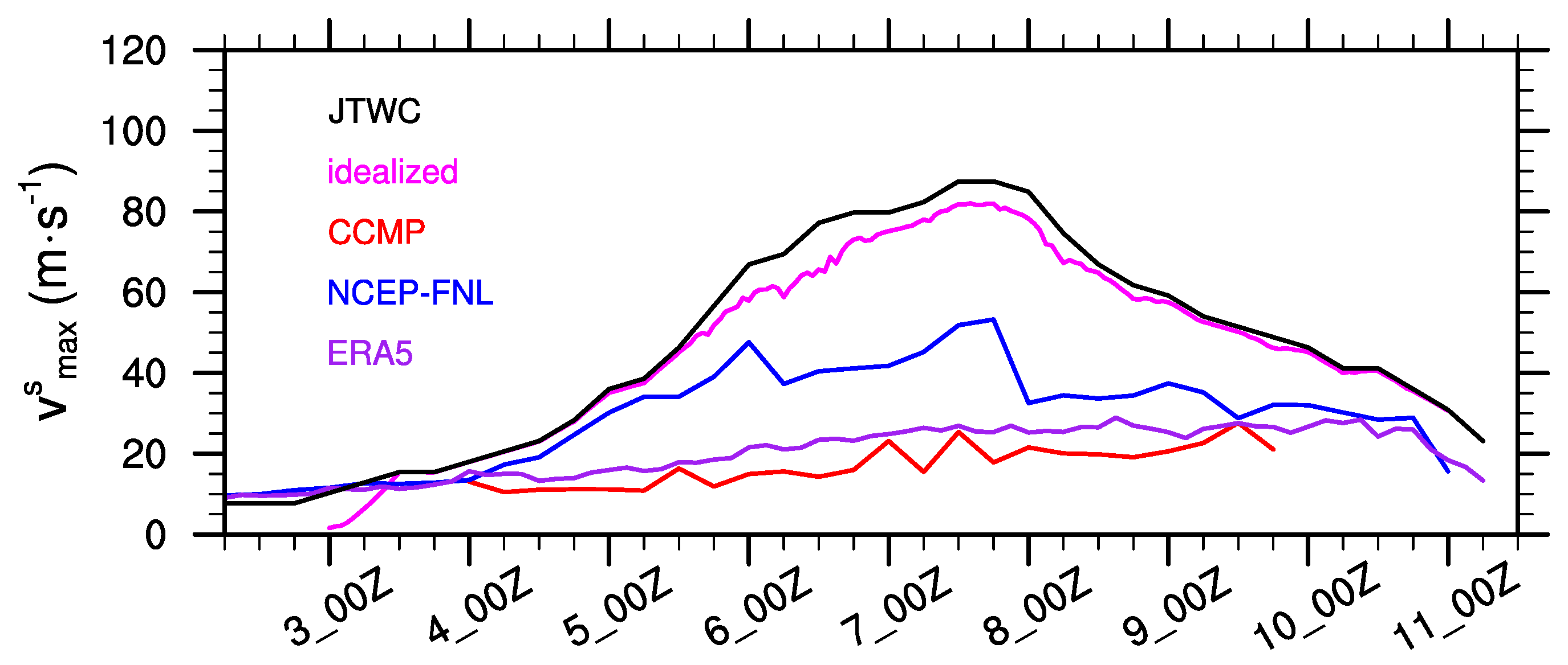
Based on the time series of JTWC best track (Figure 2), the central pressure of Haiyan began with 1010 hPa, and gradually dropped to 900 hPa. The corresponding maximum 10-min sustain wind speed increased from 7.72 to 87.45 m·s. Based on the Saffir-Simpson wind scale, Haiyan intensified to typhoon category at 5_00Z and further grew up to super-typhoon category at 6_12Z. The time period of super-typhoon intensity was 1.75 days. Later, Haiyan downgraded to typhoon category and still maintained at typhoon category for 2.5 days. On the total, Haiyan sustained typhoon category for more than 5.75 days. For the horizontal scale, the radius of typhoon eye () was roughly 10 km in typhoon category. Later, after the intensity increased to a super-typhoon category, increase to 45 km. The translation speed () was about 7 m·s at the beginning and increased to 9 m·s in the first typhoon category, and further increased to 11 m·s in the super-typhoon category. In the following second typhoon category, attained its maximum value as 11.86 m·s, and then slowed down to 7 m·s. On the maximum wind stress, the evolution of maximum wind stress generally followed the maximum wind speed, and the peak of maximum wind stress was estimated as 13.82 N·m.
3.2. SSH
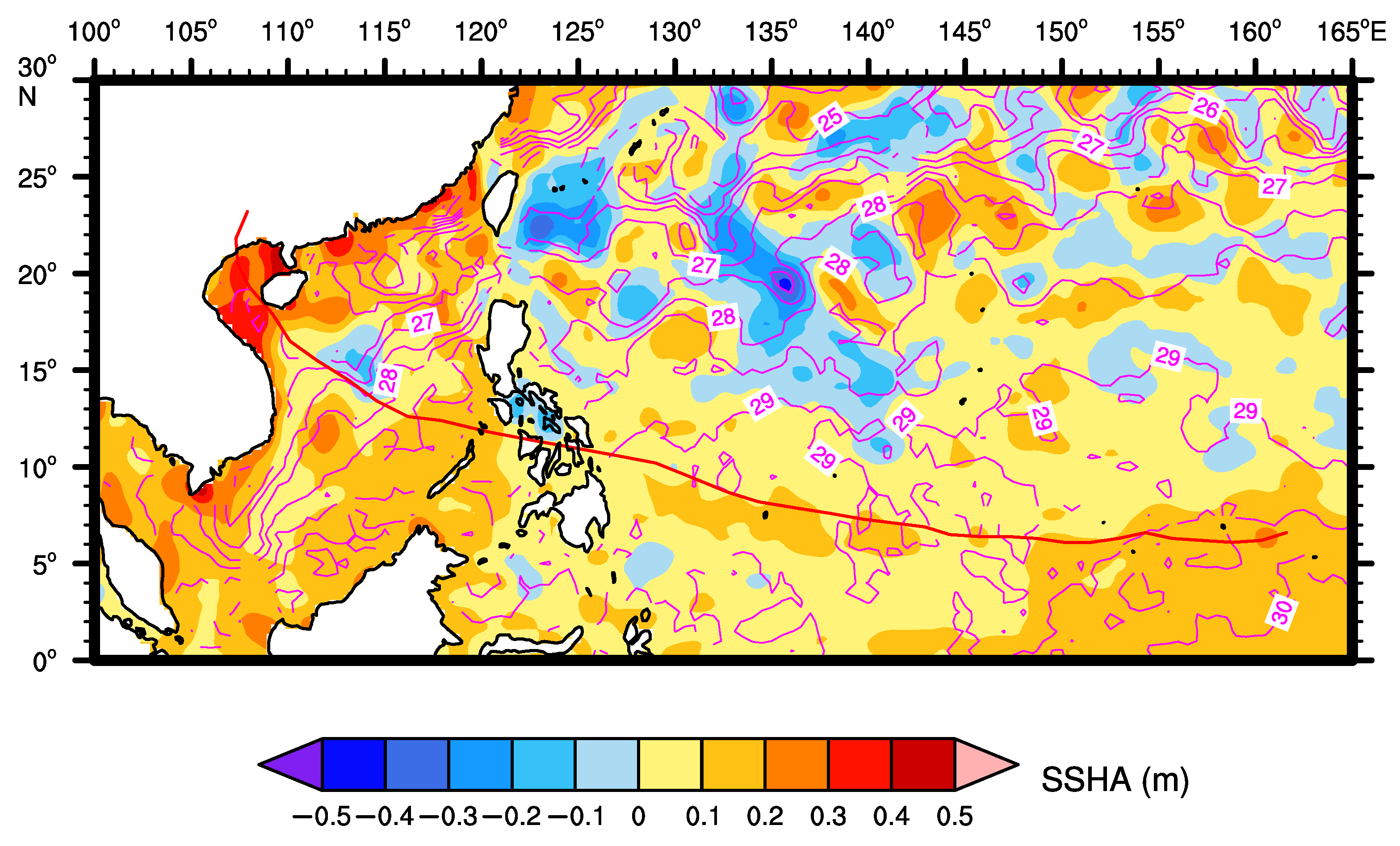
There was a positive SSH anomaly around the genesis of Haiyan (155 E, Figure 3). Later, when Haiyan moved westward to 140 E, it occurred weak meso-scale positive SSH anomaly. After entering SCS, it passed by a pair of meso-scale eddy in the central SCS (around 112 E, 13 N), as positive SSH anomaly in the left side and negative SSH anomaly in right side.
3.3. Surface Wind
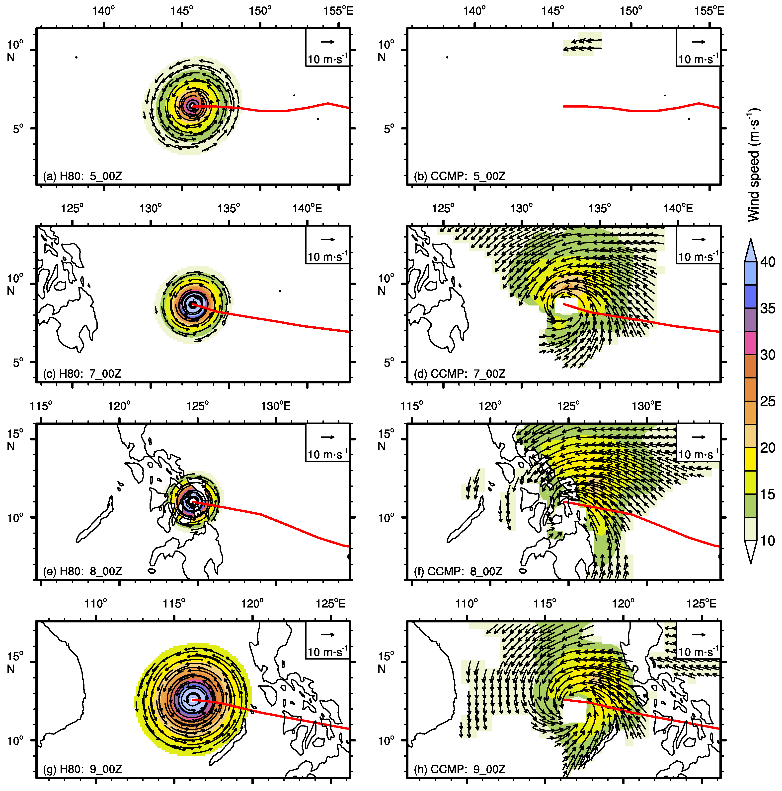
The evolution and structure of surface wind are shown in Figure 4. The idealized wind vortex reflects the best-track data in terms of the typhoon eye position, the maximum wind, and the horizontal scale of typhoon (radius of maximum wind). Satellite wind shows an alternative structure of the wind field as compared with the idealized wind vortex. Here, the core structure of the super typhoon Haiyan was described by the idealized wind vortex, which is in contrast with the satellite wind product from CCMP. Idealized wind characterized the high wind speed around the typhoon center, however, the wind speed in CCMP is relatively weak (Figure 5). At the beginning of typhoon (5_00Z), the idealized wind vortex shows an organized structure, while the wind vortex in CCMP does not exist. Later, the radius of high wind (greater than 10 m·s) decreases as in idealized wind (7_00Z and 8_00Z), and the pattern of wind vortex are identified in CCMP wind. Accordingly, the maximum winds in idealized wind vortex (CCMP) are 75 (20) and 80 (20) m·s at 7_00Z and 8_00Z respectively. After entering the SCS, the intensity of Haiyan decreases (9_00Z), while the intensity of typhoon in CCMP is still too weak (20 m·s) as compared with idealized wind vortex (60 m·s). Otherwise, CCMP shows the asymmetry structure of Haiyan. At time of 7_00Z and 8_00Z, the phenomena of right bias of surface wind is identified in CCMP, while the idealized wind vortex does not take account the asymmetric wind distribution.
Obviously, standalone satellite wind is not sufficient to provide the surface wind forcing for ocean modelling, regarding not only the horizontal coverage but also the time interval of products. Because of the clouds, time interval of repeat track orbit, space resolution, and saturated reflection problem of high wind speed, CCMP satellite products are not enough to completely describing the typhoon core, and the data quality is not high near typhoon core. In some operational occasions, it is suggested to merge the satellite wind field with other wind field like idealized vortex model.
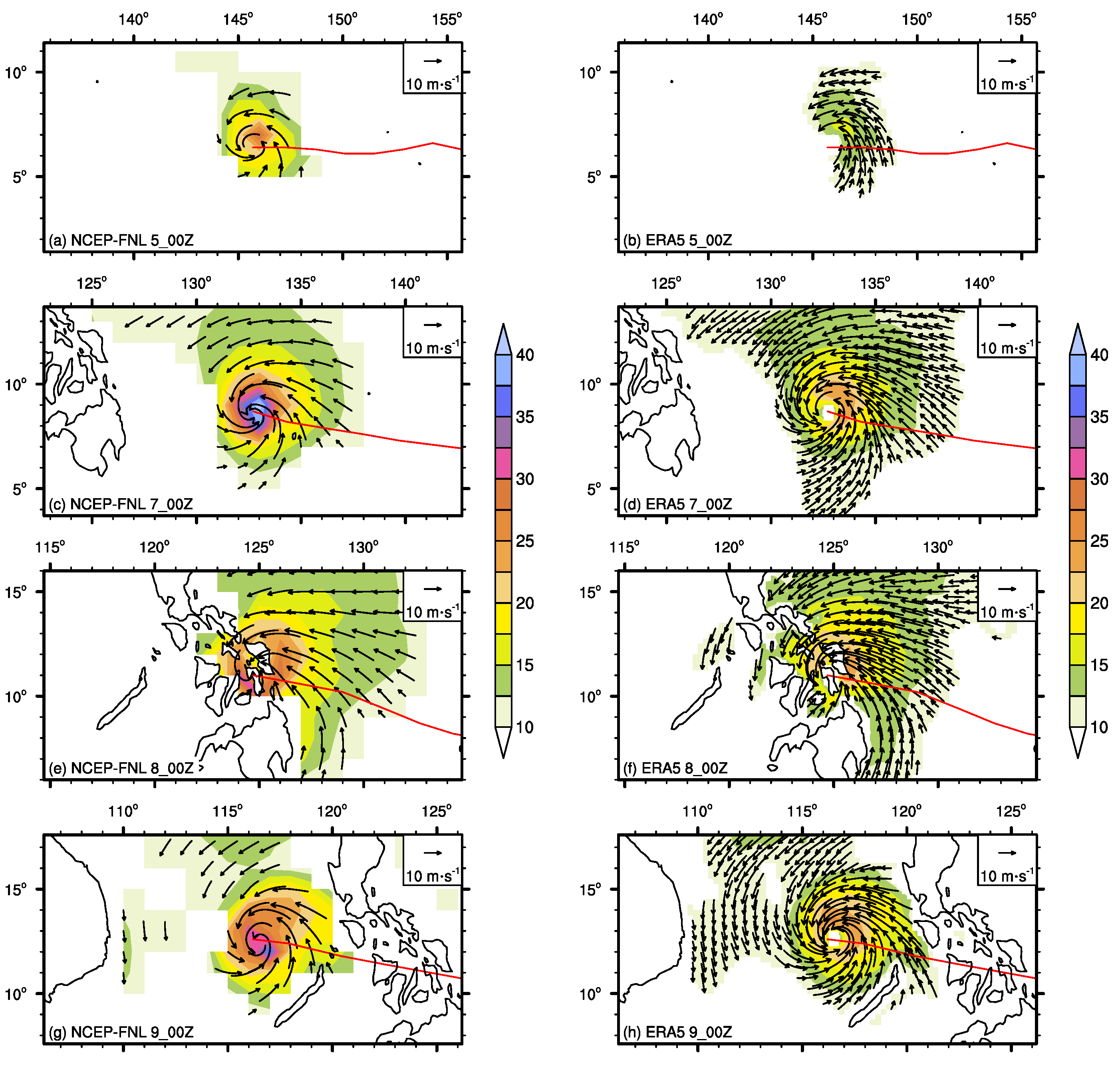
Two atmospheric analysis/reanalysis give correct central position of tropical cyclone (Figure 6). However, the intensities are different (Figure 5). The maximum wind speed of NCEP-FNL is 50 m·s, although still weaker than the idealized wind vortex (80 m·s), obviously stronger than those of CCMP and ERA5. On the spatial patterns, both NCEP-FNL and ERA5 suggest the right-bias distribution, which is consistent with the satellite wind product. The results indicate that the atmospheric analysis/reanalysis data assimilate the spatial pattern of satellite wind field.
The statistics show the bias of CCMP is −43.379 m·s, which is the highest negative bias compared with other two datasets (NCEP-FNL and ERA5; Table 2). The RMSE of CCMP attained 44.977 m·s. Therefore the wind speeds are substantially underestimated in CCMP. The performance of NCEP-FNL is relatively good, nevertheless, the bias shows −21.373 m·s and the RMSE is as high as 23.776 m·s. The CC of NCEP-FNL is 0.770. It is worthy noted that the CC of ERA5 is as lower as 0.317, and the result shows the evolution of typhoon wind is not well characterized by ERA5.
3.4. SST
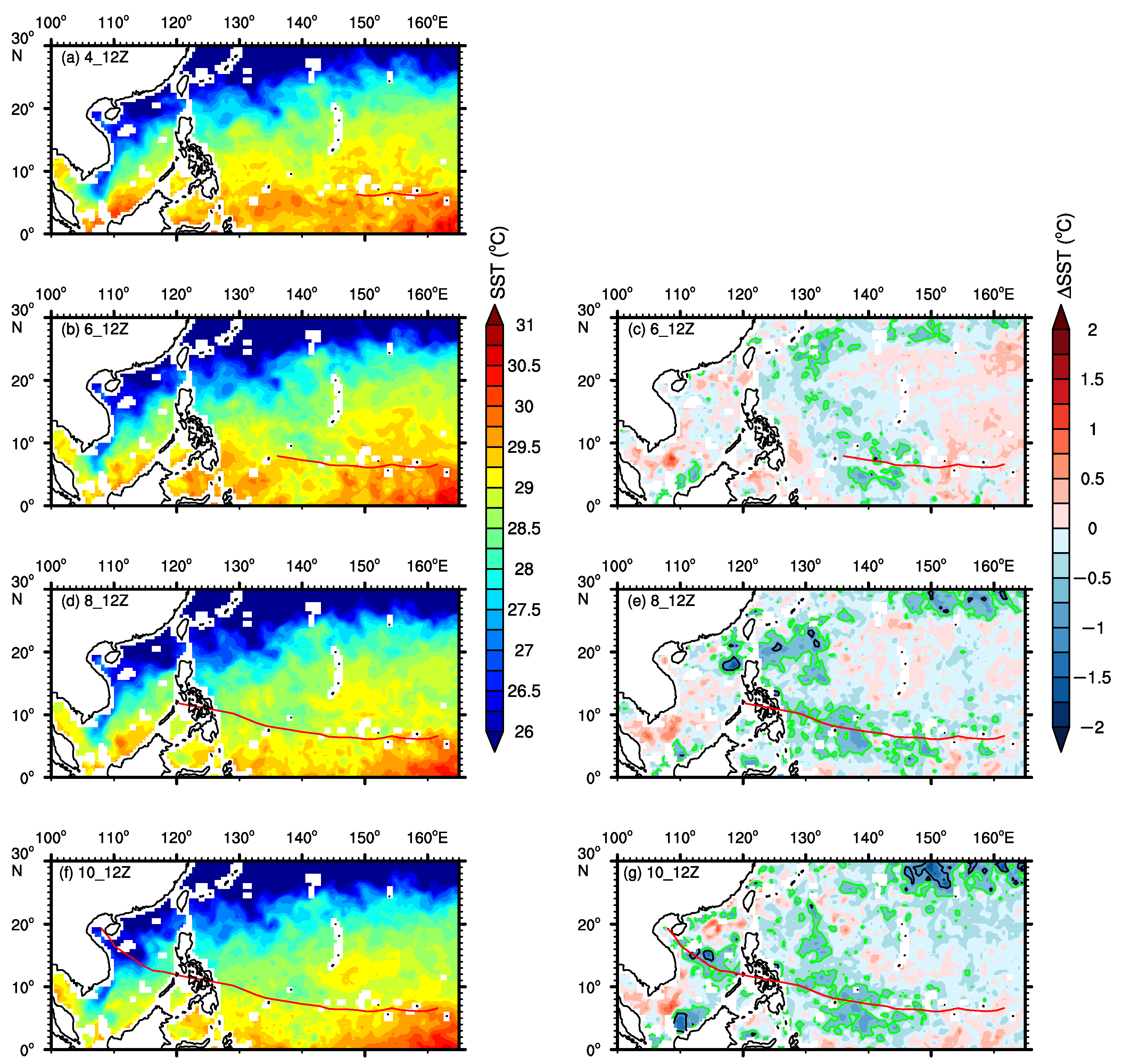
At the genesis of Haiyan, the SST along the best track was as high as 31 C as shown in satellite product (Figure 7). The SST field indicates that the track of Haiyan was along the warm water. SST was cooled by approximately 0.5 C after the typhoon passage. In the SCS, when Haiyan arrived at Hainai Island (Figure 7g), the SST cooling in the central SCS attained 1.0 C at the right side of typhoon track.
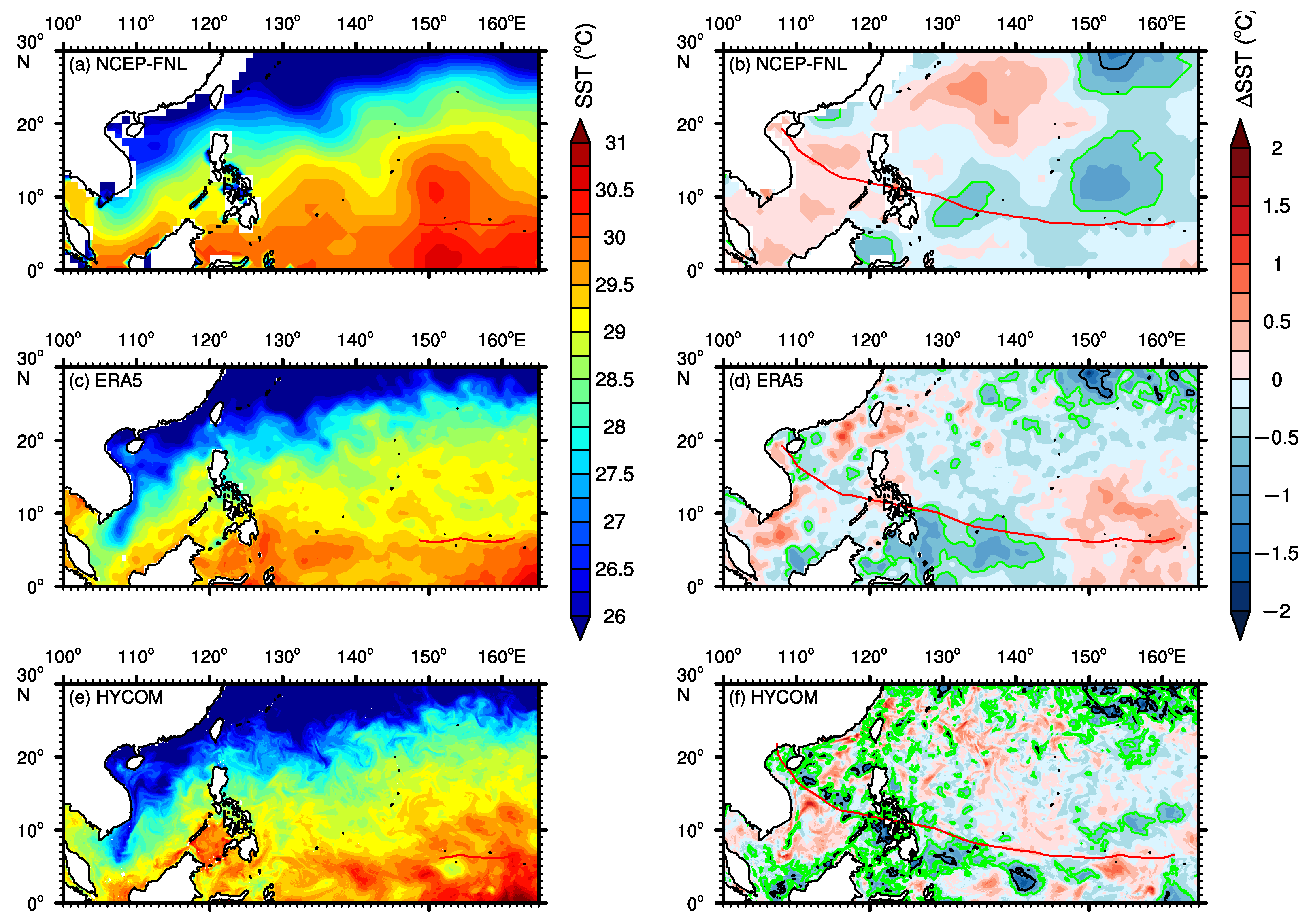
For the atmospheric and oceanic analysis/reanalysis product, Figure 8 displays the initial SST (4_12Z) and final SST change (10_12Z) in NCEP-FNL, ERA5 and HYCOM. An obvious difference is observed between NCEP-FNL and ERA5 (Figure 8a–d), that the surface water is warmer in NCEP-FNL (30.0 C) than in ERA5 (29.0 C) around the tropical cyclone genesis. Benefiting from finer horizontal resolution, ERA5 exhibits a finer horizontal structure of SST. The warmer water at the south of Mindanao Island is evident in ERA5 but not significant in NCEP-FNL. For the SST change, both NCEP-FNL and ERA5 suggest the cooling signals under typhoon track near 130 E, nonetheless, NCEP-FNL does not display the cooling at the west of Philippine Island. In addition, at the area of typhoon genesis, the SST changes are inversely different (at 150 E, 10 N), as cooling in NCEP-FNL but warming in ERA5.
In HYCOM (Figure 8e,f), the SST fields contain more information than those in atmospheric analysis/reanalysis (NCEP-FNL and ERA5). The submesoscale filaments are better represented in HYCOM due to the horizontal resolution. Besides, as compared with ERA5, HYCOM suggests: (1) Eastern shift of warm water patch from 130 E to 140 E around typhoon track, (2) cooler SST at south of Mindanao Island, (3) warmer SST in the Sulu Sea, and (4) intensified SST cooling under the tropical cyclone center at the beginning of typhoon Haiyan. Otherwise, the SST changes are roughly consistent between NCEP-FNL and ERA5. NCEP-FNL, ERA5 and HYCOM describe significantly SST cooling along tropical cyclone track at west of 140 E in WNP. The patterns of SST change in ERA5 and HYCOM are both left warming and right cooling near 113 E in SCS.
The SST of typhoon eye are highly related to ocean heat release to typhoon. As compared with satellite SST product, HYCOM shows lowest positive bias than NCEP-FNL and ERA5 for typhoon eye SST (Table 3). The bias between HYCOM and satellite product is 0.172 C, and the RMSE is 0.464 C. The bias of NCEP-FNL attained 0.481 C. The CCs of three datasets (NCEP-FNL, ERA5, and HYCOM) are all greater than 0.96, which shows the essential SST changes under typhoon eye are presented in three datasets.
Thus, remote sensing data could depict SST response to super-typhoon, and SST variation shows significant cooling in the typhoon center and surrounding areas (especially on the right side). At the same time, because the remote sensing SST product has the daily resolution, it can provide a good initial field for numerical models of typhoon and ocean. In contrast, the use of reanalysis data to give an initial SST is the need to select product. The results here show that there is a certain difference between the NCEP-FNL SST and the remote sensing data. Initial SST around typhoon eye at 4_12Z is 30.0 C for NCEP-FNL, but 29.25 C in remote sensing data. After the typhoon enters the SCS, the SST cooling, which is evident in remote sensing, is not shown in NCEP-FNL but shown as warming. As an atmospheric reanalysis product, ERA5 gives a relatively reasonable SST cooling process in the SCS. The ocean model HYCOM assimilates the satellite SST product, and its spatial pattern remains consistent with satellite product, although brings high resolution process like submesoscale activity. The statistics (bias and RMSE) on typhoon eye SST also reveal HYCOM is better than NCEP-FNL and ERA5.
3.5. Ocean Profiling
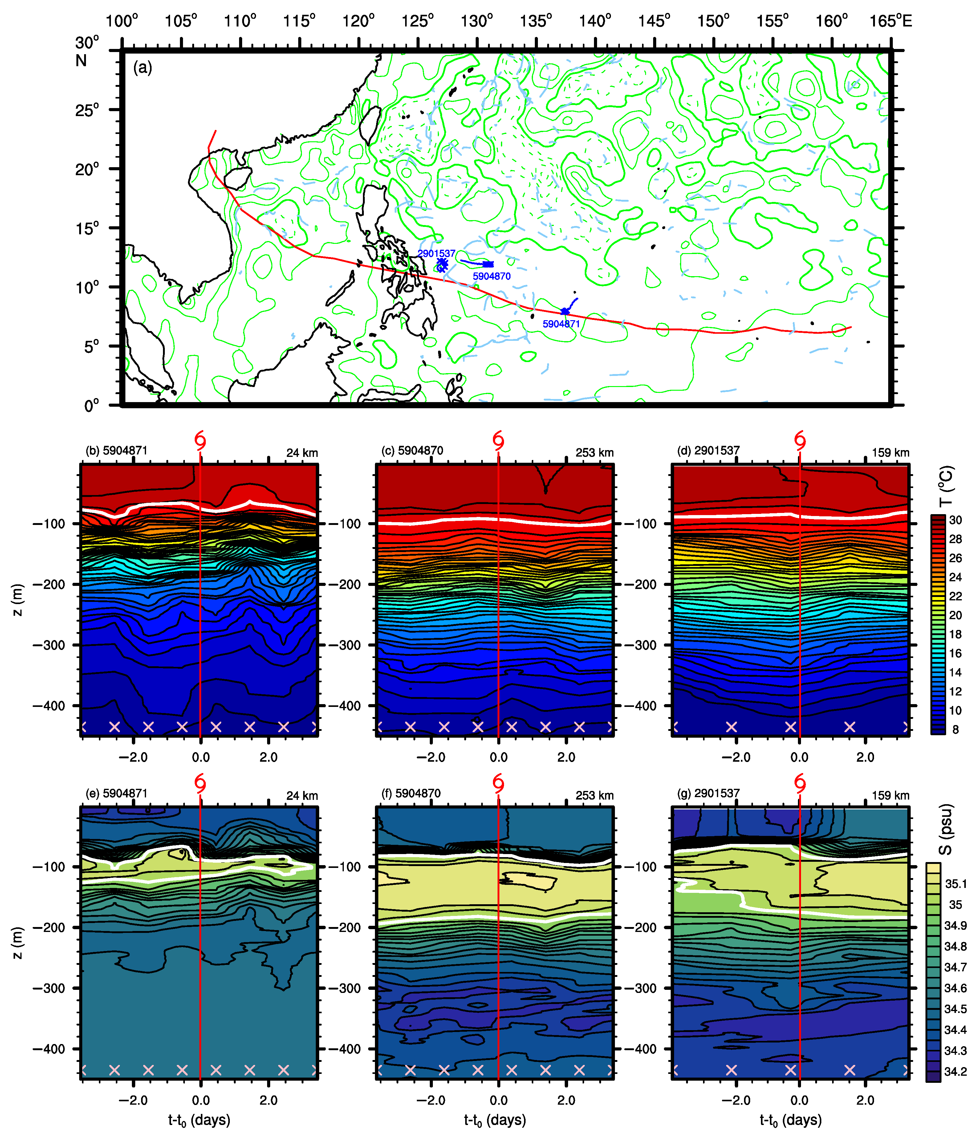
The Argo floats affected by super-typhoon Haiyan are shown in Figure 9. We also extract the SST, Sea Surface Salinity (SSS), mixed-layer depth (MLD) and isothermal depth (ITD) of Argo floats, as shown in Figure 10, and the definitions of MLD and ITD follow Wada et al. [3].
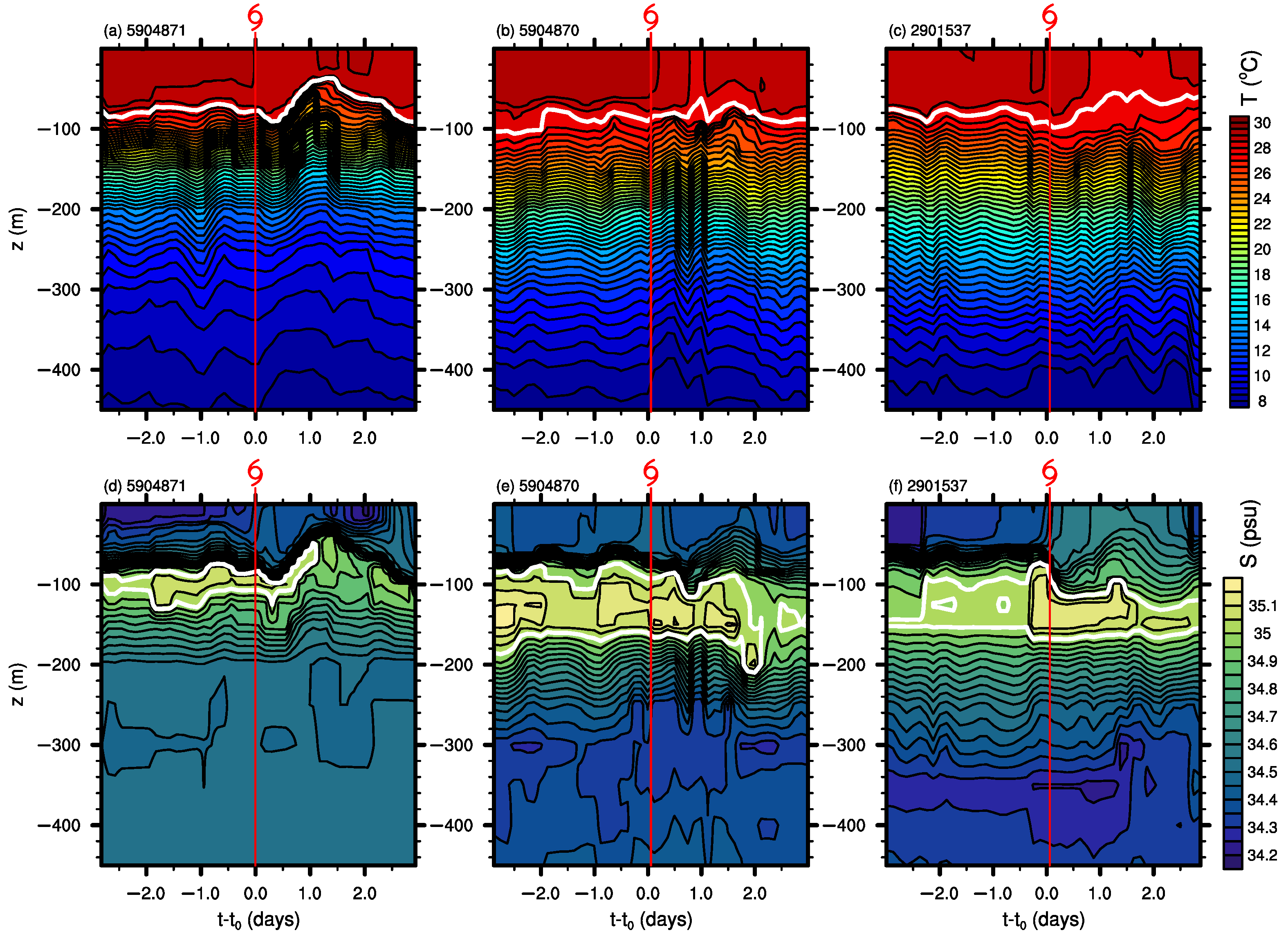
The trajectory of Argo 5904871 was very close to the typhoon track, and the minimum distance was 24 km (Figure 9a). The isotherm line of 28.5 C lifted from −80 to −40 m. The results indicate a clear upwelling occurred in the top of the thermocline and below the thermocline in the upper 300 m (Figure 9b). Under the strong wind forcing, the SST decreased roughly 0.4 C at the typhoon arrival time (Figure 10a). In the salinity evolution, the upwelling signal was also significant. Saline water was pumped up nearly 30 m at the top of thermocline. Similarly, at the typhoon arrival time, the surface freshwater was mixed with the subsurface saline water due to the wind-induced vertical mixing (Figure 9e and Figure 10d).
For Argo ID 5904870, the trajectory in the entire November was nearly parallel with typhoon track (Figure 9a). The minimum distance between Argo and typhoon was 253 km, which is relatively far compared with the radius of typhoon eye (roughly 30 km, Figure 2c). Therefore, the temperature field was not obviously changed (Figure 9c). A relatively weak downwelling was observed at 200 m in temperature evolution (1 day after typhoon arrival time). The surface salinity turned more saline due to the vertical mixing (Figure 9f and Figure 10e). Meanwhile, the downwelling at 1 day after typhoon arrival time also existed in salinity profiles at 200 m depth (Figure 9f).
For Argo ID 2901537, the trajectory was circular (Figure 9a). The minimum distance to typhoon track was 159 km. At the typhoon arrival time, the SST was slightly cooling and then recovered in one day (Figure 9d and Figure 10c). The vertical mixing induced the deeper saline water to be mixed with the surface freshwater (Figure 9g and Figure 10f).
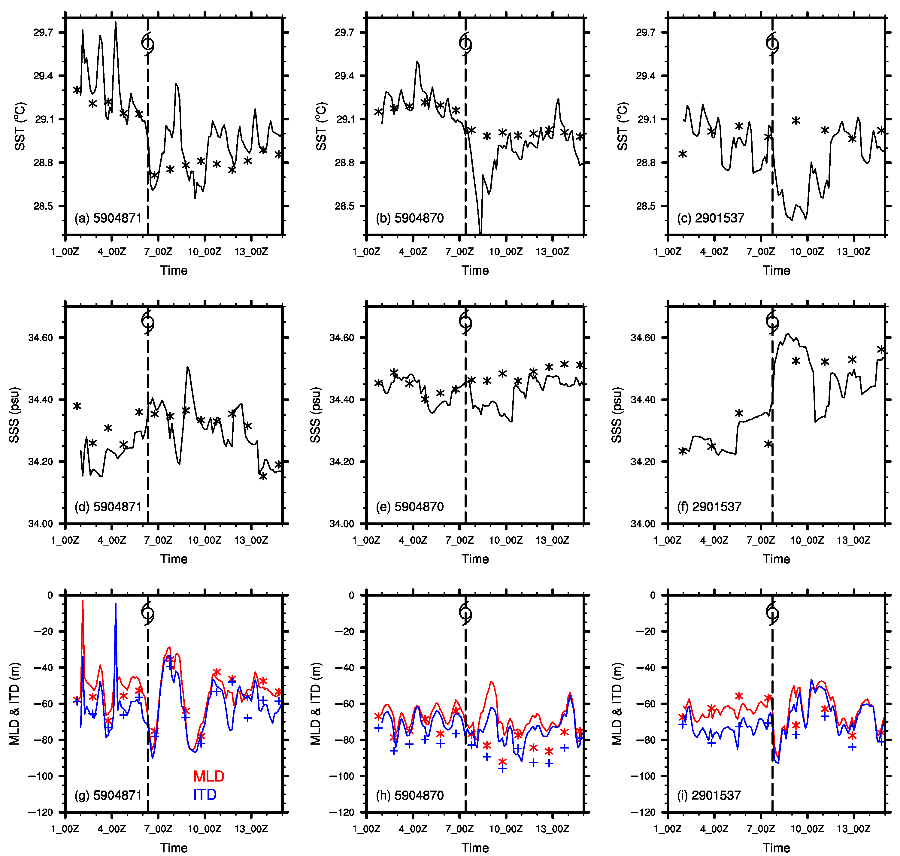
Overall, there were two Argo floats work with high sampling frequency (5904871 and 5904870), providing us with in-situ observations related to super-typhoon Haiyan [3]. The SST of 5904871 decreased from 29.1 to 28.7 C, and the depth of the mixed layer deepened from 50 to 75 m (Figure 10g). However, there was a significant oscillation in the MLD time series. This MLD oscillation was related to subsurface upwelling. When the typhoon center arrived at the observation position, near-surface Ekman transport reduced the near-surface water volume at the observation position, while subsurface water was upwelling. When the typhoon continued to move away from the observation area, the near-surface water near the typhoon center was flow out by Ekman transport, which made the near-surface water at the observation position gather, thus forced the subsurface water to downwelling to balance the pressure due to the extra surface water volume. Therefore, oscillation signals could be seen on the MLD time series. The SST cooling in these three Argo floats was not strong (Figure 10a–c; the SST cooling is lower than 0.5 C), partly due to the relatively deep MLD (Figure 10g–i; MLDs were roughly 60 m in three floats at tropical cyclone arrival time). Nevertheless, the obvious upwelling measured by Argo 5904871 provided new evidence on the upper ocean response to the typhoon.
How the ocean response to Haiyan in HYCOM? Figure 11 depicts the evolutions of temperature and salinity in HYCOM with Argo-following locations, and we compare the results with the in-situ observation directly (Figure 9). For Argo 5904871, the temperature response exhibits the subsurface upwelling, however, the upwelling signal is highly coupled in the water below the mixed-layer, which is not support in the in-situ observations, especially in the thermocline (Figure 11a). On the salinity evolution (Figure 11d), the upwelling signal is misinterpreted by HYCOM at 1 day after typhoon arrival time, that the top halocline has an intense vertical gradient, and the halocline uplifted from −100 m to −40 m. While in the observation, the vertical gradient is relatively weak, and the coupling of isohaline movement is relatively loose. Meanwhile, at 2.5 days after typhoon arrival time, there was a downwelling signal in the water depth in the range of −200 to −300 m according to Argo floats, which is also not represented in HYCOM reanalysis. There is a warming signal in SST soon after typhoon passage in HYCOM (Figure 10a and Figure 11a), while the cooling wake persists at-least 4 days in the Argo observations. The RMSE of HYCOM SST is 0.131 C (Table 4), which indicates the error of HYCOM SST is not negligible. Besides, in the HYCOM, the SSS and near-surface salinity become fresher at 2 days after typhoon arrival time, which is not evident in the Argo record. The bias of SSS is −0.026 psu, and the RMSE is 0.058 psu. The bias of MLD is as small as −0.617 m, while the bias of ITD is 1.82 m. The RMSE and CC of MLD are also better than those of ITD.
For 5904870, HYCOM overestimates the SST cooling (Figure 10b and Figure 11b). The SST cooling in HYCOM (Argo float) is 0.9 C (0.2 C). The thermocline entrainment is evident in HYCOM however almost not exist in in-situ observation. Meanwhile, high-frequency (two peaks in one day) variation as shown in HYCOM in thermocline and subsurface waters, and the signal are not resolved in the daily Argo observation. The salinity field is misinterpreted by HYCOM. The initial subsurface salinity maximum is considerable weaken in HYCOM. At 1.5 days before the typhoon arrival time, the maximum salinity at depth 130 m is 35.1 psu (Figure 9f), while 35.05 psu in HYCOM (Figure 11e). Subsequently, the high-frequency variation in halocline and subsurface water in HYCOM is not support in in-situ observation. Meanwhile, just after the typhoon pass-by, the surface salinity turned fresher in HYCOM, while the observations remain nearly unchanged (Figure 10e). Correspondingly, the top halocline uplifted considerable distance in HYCOM (Figure 11e), while the top halocline keeps steady in in-situ observation (Figure 9f). The bias of SST is roughly −0.1 C, and the RMSE is 0.148 C. The CC of SSS is as lower as 0.233, which suggests the time series of SSS in HYCOM needs to be further improved. The biases of both MLD and ITD are close to −10 m, and the CCs of MLD and ITD are lower than 0.2.
In Argo 2901537, HYCOM slightly overestimates the SST cooling (Figure 9d, Figure 10c and Figure 11c). The overestimation of SST cooling leads to −0.166 C SST bias. The RMSE of SST reaches 0.294 C. The salinity profile at typhoon arrival time is different between Argo and HYCOM, that the subsurface salinity maximum in HYCOM is higher than that in Argo observation. Subsequently, in the salinity field, a subsurface upwelling is suggested in HYCOM at 1.3 days after typhoon arrival time, but not significant in in-situ observation. For the statistics of SSS, the bias is not significant (−0.016 psu), although the RMSE is as high as 0.091 psu. The CC of SSS is 0.768, where the increase of SSS after typhoon passage keeps consistent with in-situ observations. HYCOM underestimates the MLD and ITD just after typhoon passage, which leads to the negative MLD and ITD biases. CCs of MLD and ITD are 0.438 and 0.639 respectively.
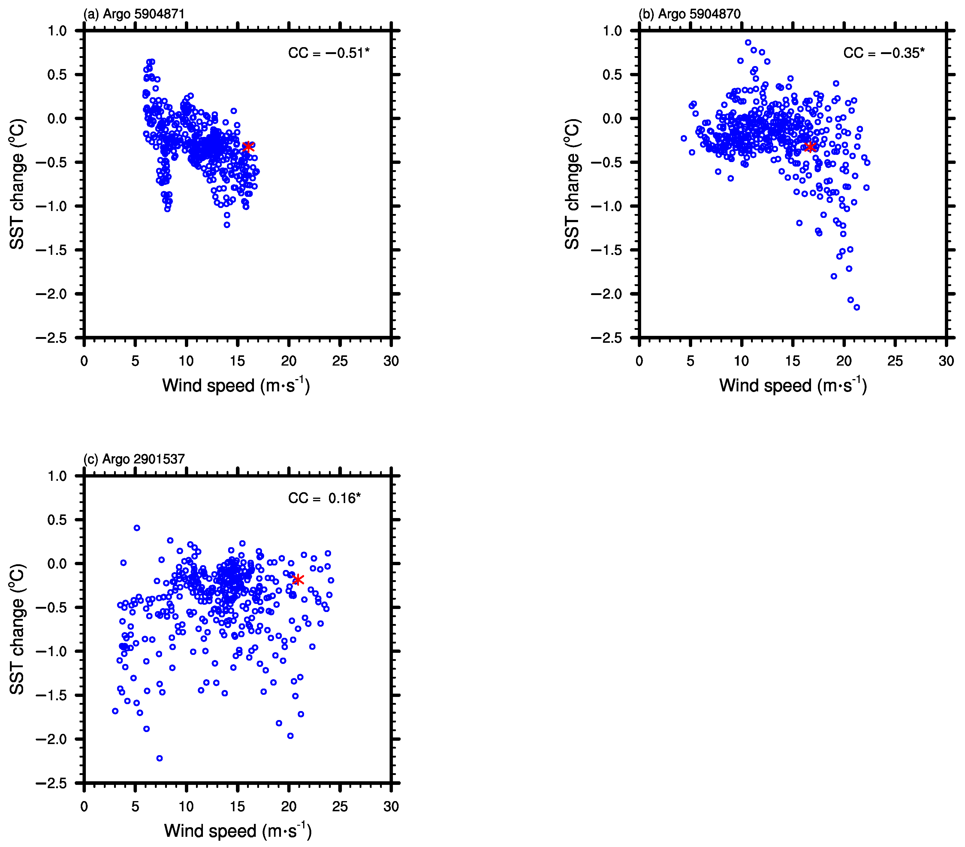
Nevertheless, as an ocean reanalysis which incorporates Argo data, HYCOM shows consistent with Argo on following aspects: (1) The time of thermocline and subsurface upwelling is close to the observation for Argo 5904871. (2) The mixed layer extension due to the wind forcing is capture by HYCOM, on temperature and salinity for Argo 5904871, as well as the salinity of Argo 2901537. (3) The dependence of SST change on surface wind are characterized in HYCOM (Figure 12). The higher wind speed indicates stronger wind stress, leads to more intensified vertical mixing. The subsurface cooler waters are more easily mixed to surface and decrease the SST. The dependence relationship is significant on Argo 5904871 and 5904870, however, the Argo close to Philippine Island (Argo 2901537) show scatter distribution, which is probably due to the influence of water depth (seafloor forcing).
Finally the performance of HYCOM is twofold. As an estimate of the ocean state, HYCOM gives a good evolution of the mixed layer due to the assimilation of satellite SST and Argo data. The CC of MLD in Argo 5904871 attains 0.915. However, due to the small amount of Argo, the initial conditions of subsurface temperature and salt profile exhibit considerable errors. Subsurface salinity maximum is 35.1 psu in Argo float, but 35.05 psu in HYCOM. The mechanics of the subsurface temperature and salt profile in HYCOM is still not sufficient. The upwelling signal in HYCOM is too strong for Argo 5904871, the vertical distance of upwelling is much higher than that of Argo, and the lifting of the subsurface isotherm and isohaline is highly coupled, while the phenomenon is not evident in the Argo float.
4. Discussion
The occurrence of super-typhoon Haiyan was partly contributed by the warm pool in WNP. The track of Haiyan kept in the low latitude helped Haiyan gained more heat flux from the ocean. The warm pool is featured by extremely warm water, and sufficiently deeper mix-layer depth. In other words, the heat content in the warm pool is considerably higher than that in the north-side ocean.
The satellite SST cooling was roughly 0.5 C in the WNP. The SST cooling was less than 0.5 C in three Argo floats. Because SST change directly influences the oceanic feedback to typhoon, negative feedback of ocean to typhoon is probably not strong in the WNP. The viewpoint is therefore consistent with existed coupled model experiment [1]. On the other hand, compared with other typhoon, SST cooling of Haiyan was relatively weak in the WNP. For instance, the composite maximum SST cooling induced by typhoon is roughly −1.4 C in the WNP [33]. The possible reasons include at-least two aspects. First, the track of typhoon Haiyan approaches the equatorial ocean, where the MLD is larger than that in the northern WNP [34]. Second, the seasonal variation of MLD in WNP is not negligible. The MLD in November is lower than those in typical typhoon season (August-to-October; [34]).
Super-typhoon Haiyan was in the decaying stage after entering the SCS, meanwhile SST response to super-typhoon Haiyan was significant in the SCS. Therefore, the oceanic negative feedback probably played roles in the fasten of typhoon decaying. Considering the SST cooling is nearly absent in NCEP-FNL, the numerical modelling of super-typhoon Haiyan with NCEP-FNL SST forcing has a risk of overestimating the air-sea heat and water vapor exchange [17,18] therefore the feedback of SST cooling to super-typhoon Haiyan would not be accounted in this kind numerical modeling.
Which wind field is suitable to drive the ocean model? Here, for the individual case of Haiyan, NCEP-FNL wind has certain rationality. The NCEP-FNL gives good eye position and relatively good typhoon intensity. NCEP-FNL is closer to best track than CCMP and ERA5 on the sense of typhoon intensity (maximum wind speed). The bias and RMSE of maximum wind speed of NCEP-FNL are −21.373 and 23.776 m·s, respectively.
The bias of salinity field is significant. The subsurface salinity maximum in HYCOM is roughly 0.05 psu lower than that in the Argo float 5904870. The corresponding SSS bias is −0.036 psu. Considering salinity plays an important role in the density stratification and the vertical mode of internal wave, the reasons of salinity bias call for further studies.
5. Conclusions
Super-typhoon Haiyan was a historical weather event. The maximum sustains wind speed attained 87.45 m·s. The corresponding peak wind stress was estimated as 13.82 N·m. Simultaneously, the SSH and SST fields reveal the super-typhoon passed over the warming region, which supplied sufficient heat and water vapor from ocean to typhoon.
The paper aims to describe the ocean response to super-typhoon Haiyan in terms of surface wind, SST and ocean profiling. The surface wind had clear right-bias at satellite product. CCMP wind suggests the high wind (greater than 10 m·s) mainly distributed at right-side of typhoon track. However, satellite wind is too weak as compared with best-track suggestions. The bias of CCMP wind is −43.379 m·s. Meanwhile, the insufficient horizontal resolution of CCMP impedes the satellite data resolve the typhoon core. Regarding the atmospheric reanalysis, For NCEP-FNL, the surface wind was better described on horizontal pattern and intensity. The bias and RMSE of NCEP-FNL wind are −21.373 and 23.776 m·s respectively. As far as the ERA5 was concerned, the typhoon intensity in ERA5 is lower than that in NCEP-FNL.
SST response to super-typhoon Haiyan is essentially described in the satellite product. The SST cooling attained 0.5 C in WNP and 1 C in SCS. In the atmospheric analysis/reanalysis, NCEP-FNL merely describes the SST cooling in SCS, while ERA5 keeps consistent with satellite product. On the other hand, in the oceanic reanalysis, SST in HYCOM follows the satellite product, and the SST in HYCOM is attributed with a finer horizontal resolution.
The results give suggestions on atmospheric modeling. Present results suggest NCEP-FNL supplies warmer SST change in the SCS. The SST differences among atmospheric analysis/reanalysis call for further investigation on the result of typhoon modelling, which are setup by different initial and boundary SST from atmospheric analysis/reanalysis.
Ocean profiling observations were achieved by Argo floats. There were two high-frequency Argo floats affected by super-typhoon Haiyan (daily sampling). One of the floats located very close to the tropical cyclone track when the tropical cyclone attained typhoon category (Argo 5904871). The ocean response was characterized by weak mixed-layer extension and strong sub-surface upwelling. Meanwhile, the second high-frequency Argo floats leaved typhoon track as 253 km (Argo 5904870), and the ocean response to typhoon Haiyan was relatively weak in both temperature and salinity evolutions. A third float with 2 days as the sampling interval was selected in the ocean response study (Argo 2901537). The mixed-layer extension as well as the halocline erosion were not negligible in this float.
The results pave road on the ocean modeling study. In the Argo-following description, HYCOM displays the mixed-layer extension and upwelling, which are roughly consistent with in-situ observations. However, the inconsistencies on the ocean response to super-typhoon Haiyan emerged as: (1) HYCOM misinterprets the thermocline and subsurface upwelling induced by typhoon Haiyan. The isohaline response in HYCOM is highly coupled at the top of isohaline, but not supported by observation. (2) There is some high-frequency variation in HYCOM after typhoon passage, the signals are not contained in the Argo records and need to be further checked. Furthermore, HYCOM has a risk of setting wrong initial condition, the subsurface salinity maximum is considerably weaker (roughly 0.05 psu lower) than that in in-situ observation of Argo 5904870.
Author Contributions
Conceptualization, S.L. and H.H.; methodology, H.H., H.Y. and Z.L.; software, H.H. and Z.L.; validation, S.L. and H.H.; formal analysis, T.E.O.; investigation, H.H.; resources, S.L. and Z.L.; data curation, T.E.O. and S.L.; writing—original draft preparation, T.E.O. and H.H.; writing—review and editing, H.H., S.L., H.Y.and Z.L.; visualization, T.E.O. and H.H.; supervision, S.L.; project administration, S.L.; funding acquisition, S.L. and H.H. All authors have read and agreed to the published version of the manuscript.
Funding
The study is funded by the Oceanic Interdisciplinary Program of Shanghai Jiao Tong University (project number SL2020MS030), and the National Natural Science Foundation of China (Nos. 41730535, 41830533).
Data Availability Statement
Best track data were downloaded from https://www.ncdc.noaa.gov/ibtracs/ (last access: 9 July 2019). The Ssalto/Duacs altimeter products (AVISO sea surface height) was produced and distributed by the Copernicus Marine and Environment Monitoring Service (CMEMS, http://www.marine.copernicus.eu; last access: 11 January 2018). CCMP winds were provided by Remote Sensing Systems (www.remss.com; last access 29 June 2017). MW_IR OI SST data were produced by Remote Sensing Systems and sponsored by National Oceanographic Partnership Program (NOPP) and the NASA Earth Science Physical Oceanography Program (www.remss.com; last access: 25 August 2019). Argo data were collected and made freely available by the International Argo Program and the national programs that contribute to it (http://www.argo.ucsd.edu, http://argo.jcommops.org), and the Argo Program is part of the Global Ocean Observing System (last access: 12 July 2019). NCEP-FNL data are available at https://rda.ucar.edu/datasets/ds083.2/ (last access: 21 July 2019). ERA5 reanalysis was generated using Copernicus Climate Change Service Information [2019]. The website is https://www.ecmwf.int/en/forecasts/datasets/reanalysis-datasets/era5 (last access 11 December 2018). HYCOM data are publicly available at http://hycom.org (last access: 27 August 2019).
Conflicts of Interest
The authors declare no conflict of interest.
References
- Mogensen, K.S.; Magnusson, L.; Bidlot, J.R. Tropical cyclone sensitivity to ocean coupling in the ECMWF coupled model. J. Geophys. Res. Ocean. 2017, 122, 4392–4412. [Google Scholar] [CrossRef]
- Bushnell, J.M.; Cherrett, R.C.; Falvey, R.J. Joint Typhoon Warning Center Annual Tropical Cyclone Report 2018; Report; Joint Typhoon Warning Center: Honolulu, HI, USA, 2018. [Google Scholar]
- Wada, A.; Uehara, T.; Ishizaki, S. Typhoon-induced sea surface cooling during the 2011 and 2012 typhoon seasons: Observational evidence and numerical investigations of the sea surface cooling effect using typhoon simulations. Prog. Earth Planet. Sci. 2014, 1. [Google Scholar] [CrossRef] [Green Version]
- Sun, J.; He, H.; Hu, X.; Wang, D.; Gao, C.; Song, J. Numerical Simulations of Typhoon Hagupit (2008) Using WRF. Weather Forecast. 2019, 34, 999–1015. [Google Scholar] [CrossRef]
- Price, J.F. Upper Ocean Response to a Hurricane. J. Phys. Oceanogr. 1981, 11, 153–175. [Google Scholar] [CrossRef] [Green Version]
- Emanuel, K. Tropical Cyclones. Annu. Rev. Earth Planet. Sci. 2003, 31, 75–104. [Google Scholar] [CrossRef]
- Chan, J.C.L.; Duan, Y.; Shay, L.K. Tropical Cyclone Intensity Change from a Simple Ocean–Atmosphere Coupled Model. J. Atmos. Sci. 2001, 58, 154–172. [Google Scholar] [CrossRef]
- Liu, B.; Liu, H.; Xie, L.; Guan, C.; Zhao, D. A Coupled Atmosphere–Wave–Ocean Modeling System: Simulation of the Intensity of an Idealized Tropical Cyclone. Mon. Weather Rev. 2011, 139, 132–152. [Google Scholar] [CrossRef]
- Ning, J.; Xu, Q.; Feng, T.; Zhang, H.; Wang, T. Upper Ocean Response to Two Sequential Tropical Cyclones over the Northwestern Pacific Ocean. Remote Sens. 2019, 11, 2431. [Google Scholar] [CrossRef] [Green Version]
- Ning, J.; Xu, Q.; Zhang, H.; Wang, T.; Fan, K. Impact of Cyclonic Ocean Eddies on Upper Ocean Thermodynamic Response to Typhoon Soudelor. Remote Sens. 2019, 11, 938. [Google Scholar] [CrossRef] [Green Version]
- Lin, I.I.; Pun, I.F.; Lien, C.C. “Category-6” supertyphoon Haiyan in global warming hiatus: Contribution from subsurface ocean warming. Geophys. Res. Lett. 2014, 41, 8547–8553. [Google Scholar] [CrossRef]
- Huang, H.C.; Boucharel, J.; Lin, I.I.; Jin, F.F.; Lien, C.C.; Pun, I.F. Air-sea fluxes for Hurricane Patricia (2015): Comparison with supertyphoon Haiyan (2013) and under different ENSO conditions. J. Geophys. Res. Ocean. 2017, 122, 6076–6089. [Google Scholar] [CrossRef]
- Liu, Z.; Hou, Y.; Xie, Q.; Hu, P.; Liu, Y. The upper-ocean response to typhoons as measured at a moored acoustic Doppler current profiler. Chin. J. Ocean. Limnol. 2015, 33, 1256–1264. [Google Scholar] [CrossRef]
- Guan, S.; Liu, Z.; Song, J.; Hou, Y.; Feng, L. Upper ocean response to Super Typhoon Tembin (2012) explored using multiplatform satellites and Argo float observations. Int. J. Remote Sens. 2017, 38, 5150–5167. [Google Scholar] [CrossRef]
- Yue, X.; Zhang, B.; Liu, G.; Li, X.; Zhang, H.; He, Y. Upper Ocean Response to Typhoon Kalmaegi and Sarika in the South China Sea from Multiple-Satellite Observations and Numerical Simulations. Remote Sens. 2018, 10, 348. [Google Scholar] [CrossRef] [Green Version]
- Chen, H.; Li, S.; He, H.L.; Song, J.B.; Ling, Z.; Cao, A.Z.; Zou, Z.S.; Qiao, W.L. Observational study of the coupled atmosphere-ocean system for super-typhoon Meranti using satellite, surface drifter, Argo float, and reanalysis data. Acta Oceanol. Sin. 2021, 40, 70–84. [Google Scholar] [CrossRef]
- Li, F.N.; Song, J.B.; He, H.L.; Li, S.; Li, X.; Guan, S.D. Assessment of surface drag coefficient parametrizations based on observations and simulations using the Weather Research and Forecasting model. Atmos. Ocean. Sci. Lett. 2016, 9, 327–336. [Google Scholar] [CrossRef] [Green Version]
- Li, F.; Song, J.; Li, X. A preliminary evaluation of the necessity of using a cumulus parameterization scheme in high-resolution simulations of Typhoon Haiyan (2013). Nat. Hazards 2018, 92, 647–671. [Google Scholar] [CrossRef]
- Wada, A.; Kanada, S.; Yamada, H. Effect of Air-Sea Environmental Conditions and Interfacial Processes on Extremely Intense Typhoon Haiyan (2013). J. Geophys. Res. Atmos. 2018, 123, 10379–10405. [Google Scholar] [CrossRef]
- Kueh, M.T.; Chen, W.M.; Sheng, Y.F.; Lin, S.C.; Wu, T.R.; Yen, E.; Tsai, Y.L.; Lin, C.Y. Effects of horizontal resolution and air–sea flux parameterization on the intensity and structure of simulated Typhoon Haiyan (2013). Nat. Hazards Earth Syst. Sci. 2019, 19, 1509–1539. [Google Scholar] [CrossRef] [Green Version]
- Knapp, K.R.; Kruk, M.C.; Levinson, D.H.; Diamond, H.J.; Neumann, C.J. The International Best Track Archive for Climate Stewardship (IBTrACS): Unifying Tropical Cyclone Data. Bull. Am. Meteorol. Soc. 2010, 91, 363–376. [Google Scholar] [CrossRef]
- Ubelmann, C.; Klein, P.; Fu, L.L. Dynamic Interpolation of Sea Surface Height and Potential Applications for Future High-Resolution Altimetry Mapping. J. Atmos. Ocean. Technol. 2015, 32, 177–184. [Google Scholar] [CrossRef] [Green Version]
- Atlas, R.; Hoffman, R.N.; Ardizzone, J.; Leidner, S.M.; Jusem, J.C.; Smith, D.K.; Gombos, D. A cross-calibrated, multiplatform ocean surface wind velocity product for meteorological and oceanographic applications. Bull. Am. Meteorol. Soc. 2011, 92, 157–174. [Google Scholar] [CrossRef]
- Woo, H.J.; Park, K.A. Inter-Comparisons of Daily Sea Surface Temperatures and In-Situ Temperatures in the Coastal Regions. Remote Sens. 2020, 12, 1592. [Google Scholar] [CrossRef]
- Riser, S.C.; Freeland, H.J.; Roemmich, D.; Wijffels, S.; Troisi, A.; Belbéoch, M.; Gilbert, D.; Xu, J.; Pouliquen, S.; Thresher, A.; et al. Fifteen years of ocean observations with the global Argo array. Nat. Clim. Chang. 2016, 6, 145–153. [Google Scholar] [CrossRef] [Green Version]
- Cummings, J.A. Operational multivariate ocean data assimilation. Q. J. R. Meteorol. Soc. 2005, 131, 3583–3604. [Google Scholar] [CrossRef] [Green Version]
- Cummings, J.A.; Smedstad, O.M. Variational Data Assimilation for the Global Ocean. In Data Assimilation for Atmospheric, Oceanic and Hydrologic Applications (Vol. II); Park, S.K., Xu, L., Eds.; Springer: Berlin/Heidelberg, Germany, 2013; pp. 303–343. [Google Scholar] [CrossRef]
- Xu, Y.; He, H.; Song, J.; Hou, Y.; Li, F. Observations and Modeling of Typhoon Waves in the South China Sea. J. Phys. Oceanogr. 2017, 47, 1307–1324. [Google Scholar] [CrossRef]
- Qiao, W.; Song, J.; He, H.; Li, F. Application of different wind field models and wave boundary layer model to typhoon waves numerical simulation in WAVEWATCH III model. Tellus A Dyn. Meteorol. Oceanogr. 2019, 71, 1657552. [Google Scholar] [CrossRef] [Green Version]
- Pu, Z.X.; Braun, S.A. Evaluation of Bogus Vortex Techniques with Four-Dimensional Variational Data Assimilation. Mon. Weather Rev. 2001, 129, 2023–2039. [Google Scholar] [CrossRef]
- Holland, G.J. An Analytic Model of the Wind and Pressure Profiles in Hurricanes. Mon. Weather Rev. 1980, 108, 1212–1218. [Google Scholar] [CrossRef]
- Moon, I.J.; Ginis, I.; Hara, T.; Thomas, B. A physics-based parameterization of air–sea momentum flux at high wind speeds and its impact on hurricane intensity predictions. Mon. Wea. Rev. 2007, 135, 2869–2878. [Google Scholar] [CrossRef] [Green Version]
- Wang, G.; Wu, L.; Johnson, N.C.; Ling, Z. Observed three-dimensional structure of ocean cooling induced by Pacific tropical cyclones. Geophys. Res. Lett. 2016, 43, 7632–7638. [Google Scholar] [CrossRef]
- Clement, B.M.; Gurvan, M.; Albert, F.S.; Alban, L.; Daniele, L. Mixed layer depth over the global ocean: An examination of profile data and a profile-based climatology. J. Geophys. Res. Ocean. 2004, 109. [Google Scholar] [CrossRef]
Figure 1.
Best track of super-typhoon Haiyan showing the trajectory and the intensity.

Figure 2.
Time series of best-track information of super-typhoon Haiyan, (a) central pressure, (b) maximum sustain wind speed, (c) radius of eye, (d) translation speed, and (e) wind stress. The light gray shade indicates the time period of typhoon (TY) stage and the deep gray shade represents super-typhoon (STY) stage.

Figure 3.
Sea surface height anomaly during super-typhoon Haiyan (color shading), the sea surface temperature (contour), and the best track data (thick red line).
Figure 3.
Sea surface height anomaly during super-typhoon Haiyan (color shading), the sea surface temperature (contour), and the best track data (thick red line).

Figure 4.
Wind fields of super-typhoon Haiyan with the red line indicating the best track of Haiyan. Left panels (a,c,e,g) are built from idealized wind vortex, while the right panels (b,d,f,h) are provided by satellite CCMP wind.
Figure 4.
Wind fields of super-typhoon Haiyan with the red line indicating the best track of Haiyan. Left panels (a,c,e,g) are built from idealized wind vortex, while the right panels (b,d,f,h) are provided by satellite CCMP wind.

Figure 5.
Time series of maximum surface wind during super-typhoon Haiyan. The data sources include the best-track data of JTWC (the maximum sustained wind is used), idealized wind vortex, satellite wind of CCMP, analysis wind of NCEP-FNL, and reanalysis wind provided by ERA5.
Figure 5.
Time series of maximum surface wind during super-typhoon Haiyan. The data sources include the best-track data of JTWC (the maximum sustained wind is used), idealized wind vortex, satellite wind of CCMP, analysis wind of NCEP-FNL, and reanalysis wind provided by ERA5.

Figure 6.
Wind fields of super-typhoon Haiyan in atmospheric analysis/reanalysis. (a,c,e,g), NCEP-FNL, (b,d,f,h) ERA5.
Figure 6.
Wind fields of super-typhoon Haiyan in atmospheric analysis/reanalysis. (a,c,e,g), NCEP-FNL, (b,d,f,h) ERA5.

Figure 7.
Satellite-based sea surface temperature during super-typhoon Haiyan. Left panels (a,b,d,f) show the sea surface temperature at 4_12Z, 6_12Z, 8_12Z and 10_12Z respectively. Right panels (c,e,g) are the sea surface temperature change for 6_12Z, 8_12Z and 10_12Z respectively, where the initial time is set as 4_12Z. The contours represent 0.5 C (green) and 1.0 C (black) cooling.

Figure 8.
Sea surface temperature during super-typhoon Haiyan in atmospheric and oceanic analysis/reanalysis. (a,b) NCEP-FNL, (c,d) ERA5, (e,f) HYCOM. Left panels (a,c,e) are the initial SST for typhoon Haiyan (4_12Z), and right panels (b,d,f) are the SST change after the passage of typhoon Haiyan (10_12Z). The contours represent 0.5 C (green) and 1.0 C (black) cooling.

Figure 9.
Argo floats affected by super-typhoon Haiyan. (a) Trajectories of all Argo float in November 2013 (light blue lines), and the three selected Argo floats for detailed analysis (blue lines). The blue crosses denote the records within 4 days before and after typhoon arrival time. The red solid line is the best-track of Haiyan (JTWC). (b–d) Profiling observations of temperature from Argo ID 5904871, 5904870 and 2901537, respectively. The x coordinates are the relative time referred to the arrival time of typhoon (), the pink crosses represent the Argo sampling time. The minimum distances between Argo and typhoon are given at the top-right of subfigures. The isothermal line of 28 C is highlighted as thick white line. (e–g) as in (b–d) but for salinity. The isohaline of 35.0 psu is highlighted as thick white line.

Figure 10.
Time series of sea surface temperature (SST; (a–c)), sea surface salinity (SSS; (d–f)), mixed-layer depth (MLD; (g–i)), and isothermal depth (ITD; (g–i)) in Argo record during super-typhoon Haiyan. Left panels (a,d,g) Argo float 5904871. Middle panels (b,e,h) Argo float 5904870. Right panels (c,f,i) Argo float 2901537. The markers are from Argo in-situ observation, and the solid lines represent HYCOM results. In (g–i), the red asterisks and blue pluses are the MLDs and ITDs in Argo floats, respectively.

Figure 11.
Ocean response to super-typhoon Haiyan in oceanic reanalysis HYCOM. The data are interpolated to Argo-following grids, as in Figure 9. (a–c) Profiling observations of temperature in HYCOM for Argo ID 5904871, 5904870 and 2901537, respectively. (d–f) The corresponding salinity profiles in HYCOM.

Figure 12.
Dependence of SST change on surface wind speed around Argo float. (a–c) are for Argo float 5904871, 5904870, 2901537 respectively. SST change is adopted from HYCOM dataset, and surface wind speed is based on NCEP-FNL. The blue dots are the results within 5 around typhoon eye. The red asterisk are the Argo observations on SST change. The SST change is defined as SST difference between the times after and prior to typhoon arrival time by quarter inertial period. The surface wind speed is the mean wind speed during the correspond time period. CC is the correlation coefficient. The asterisk in CC represents the CC passing 0.05 significant test.


Table 1.
Multiplatform datasets used in present study. CTD represents conductivity (or salinity), temperature and depth.
Table 1.
Multiplatform datasets used in present study. CTD represents conductivity (or salinity), temperature and depth.
| Variable | Dataset | Version | Resolution |
|---|---|---|---|
| Best track | JTWC in IBTrACS | V03r10 | 6 hourly |
| SSH | AVISO | V5.1 | 1/4 × 1/4, daily |
| wind | CCMP | V2.0 | daily |
| wind, SST | NCEP-FNL | 1 × 1, 6-hourly | |
| wind, SST | ERA5 | 1/4 × 1/4, 3-hourly | |
| SST | MW_IR OISST | V02.0 | 9 km, 6-hourly |
| CTD field | HYCOM | GOFS3.1:GLBv0.08 | 1/12 × 1/12, 3-hourly |
| CTD profile | Argo | float-dependent |
Table 2.
Statistics on surface wind evaluation (unit: m·s). The base dataset is idealized wind vortex. The comparisons are performed during typhoon period. The asterisk in CC represents the CC passing 0.05 significant test.
Table 2.
Statistics on surface wind evaluation (unit: m·s). The base dataset is idealized wind vortex. The comparisons are performed during typhoon period. The asterisk in CC represents the CC passing 0.05 significant test.
| Dataset | Bias | RMSE | CC |
|---|---|---|---|
| CCMP | −43.379 | 44.977 | 0.621 * |
| NCEP-FNL | −21.373 | 23.776 | 0.770 * |
| ERA5 | −34.392 | 37.116 | 0.317 |
Table 3.
Statistics on SST evaluation (unit: C). The base dataset is satellite MW_IR OISST product. The comparisons are performed during 2 November to 10 November. The SST of typhoon eye is considered. The asterisk in CC represents the CC passing 0.05 significant test.
Table 3.
Statistics on SST evaluation (unit: C). The base dataset is satellite MW_IR OISST product. The comparisons are performed during 2 November to 10 November. The SST of typhoon eye is considered. The asterisk in CC represents the CC passing 0.05 significant test.
| Dataset | Bias | RMSE | CC |
|---|---|---|---|
| NCEP-FNL | 0.481 | 0.584 | 0.975 * |
| ERA5 | 0.222 | 0.425 | 0.971 * |
| HYCOM | 0.172 | 0.464 | 0.967 * |
Table 4.
Statistics on SST (unit: C), SSS (unit: psu), MLD (unit: m) and ITD (unit: m) between Argo float and HYCOM.The comparisons are performed during 2 November to 15 November. The negative (positive) bias in MLD or ITD indicates the depth in HYCOM is shallower (deeper) than that in Argo. The asterisk in CC represents the CC passing 0.05 significant test.
| Argo ID | Variable | Bias | RMSE | CC |
|---|---|---|---|---|
| 5904871 | SST | 0.033 | 0.131 | 0.787 * |
| SSS | −0.026 | 0.058 | 0.776 * | |
| MLD | −0.617 | 5.320 | 0.915 * | |
| ITD | 1.820 | 9.116 | 0.751 * | |
| 5904870 | SST | −0.095 | 0.148 | 0.873 * |
| SSS | −0.036 | 0.060 | 0.233 | |
| MLD | −9.620 | 13.506 | 0.186 | |
| ITD | −10.714 | 13.717 | 0.194 | |
| 2901537 | SST | −0.166 | 0.294 | 0.675 * |
| SSS | −0.016 | 0.091 | 0.768 * | |
| MLD | −4.331 | 10.413 | 0.438 | |
| ITD | −7.224 | 10.357 | 0.639 |
Publisher’s Note: MDPI stays neutral with regard to jurisdictional claims in published maps and institutional affiliations. |
© 2021 by the authors. Licensee MDPI, Basel, Switzerland. This article is an open access article distributed under the terms and conditions of the Creative Commons Attribution (CC BY) license (https://creativecommons.org/licenses/by/4.0/).
Share and Cite
MDPI and ACS Style
Oginni, T.E.; Li, S.; He, H.; Yang, H.; Ling, Z. Ocean Response to Super-Typhoon Haiyan. Water 2021, 13, 2841. https://doi.org/10.3390/w13202841
AMA Style
Oginni TE, Li S, He H, Yang H, Ling Z. Ocean Response to Super-Typhoon Haiyan. Water. 2021; 13(20):2841. https://doi.org/10.3390/w13202841
Chicago/Turabian StyleOginni, Tolulope Emmanuel, Shuang Li, Hailun He, Hongwei Yang, and Zheng Ling. 2021. "Ocean Response to Super-Typhoon Haiyan" Water 13, no. 20: 2841. https://doi.org/10.3390/w13202841
Note that from the first issue of 2016, this journal uses article numbers instead of page numbers. See further details here.