
Determining Stress State of Source Media with Identified Difference between Groundwater Level during Loading and Unloading Induced by Earth Tides

Abstract
:1. Introduction
2. Methods
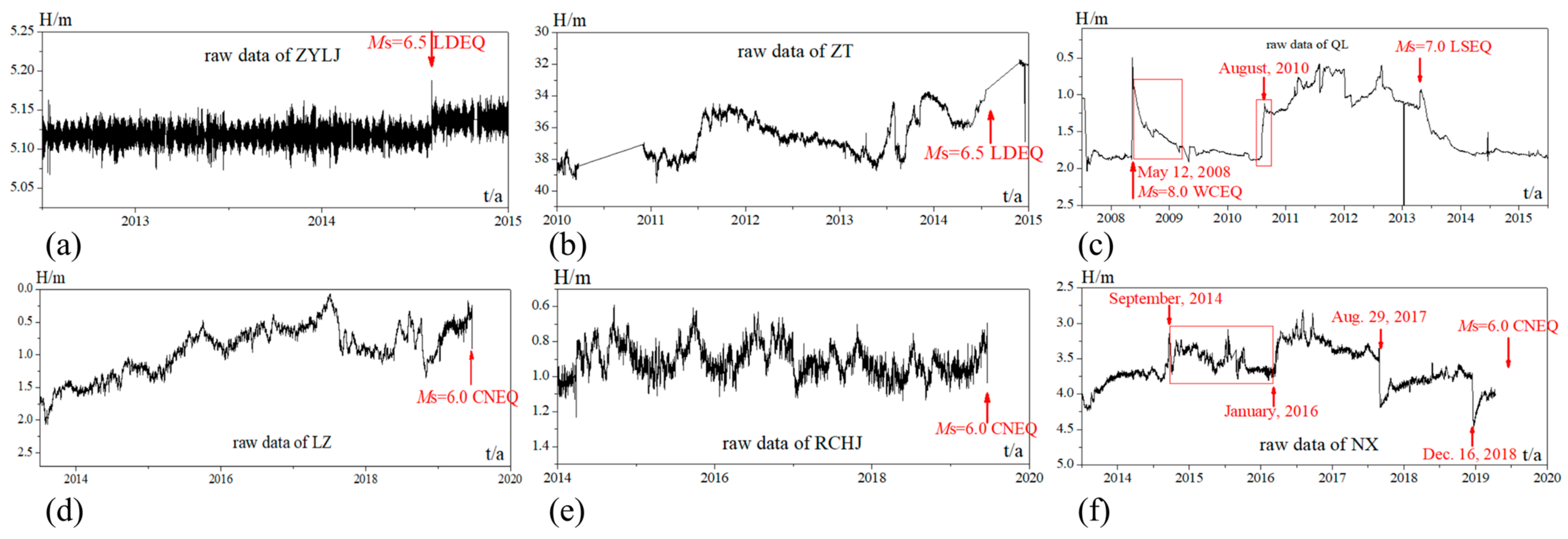
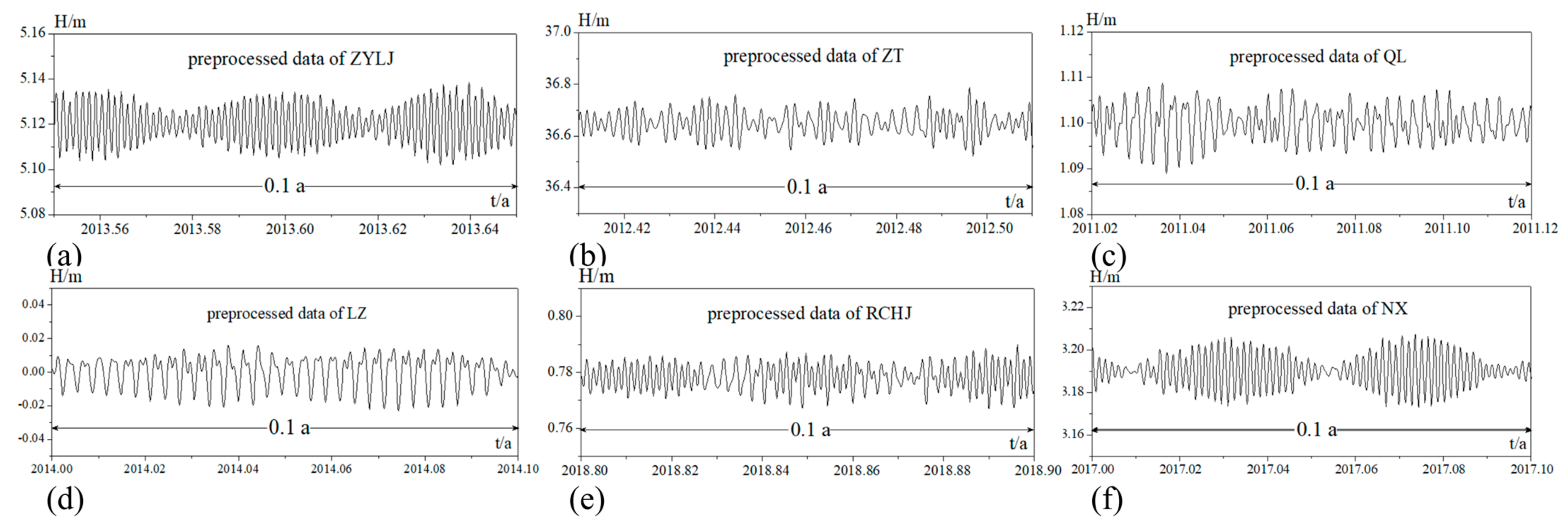
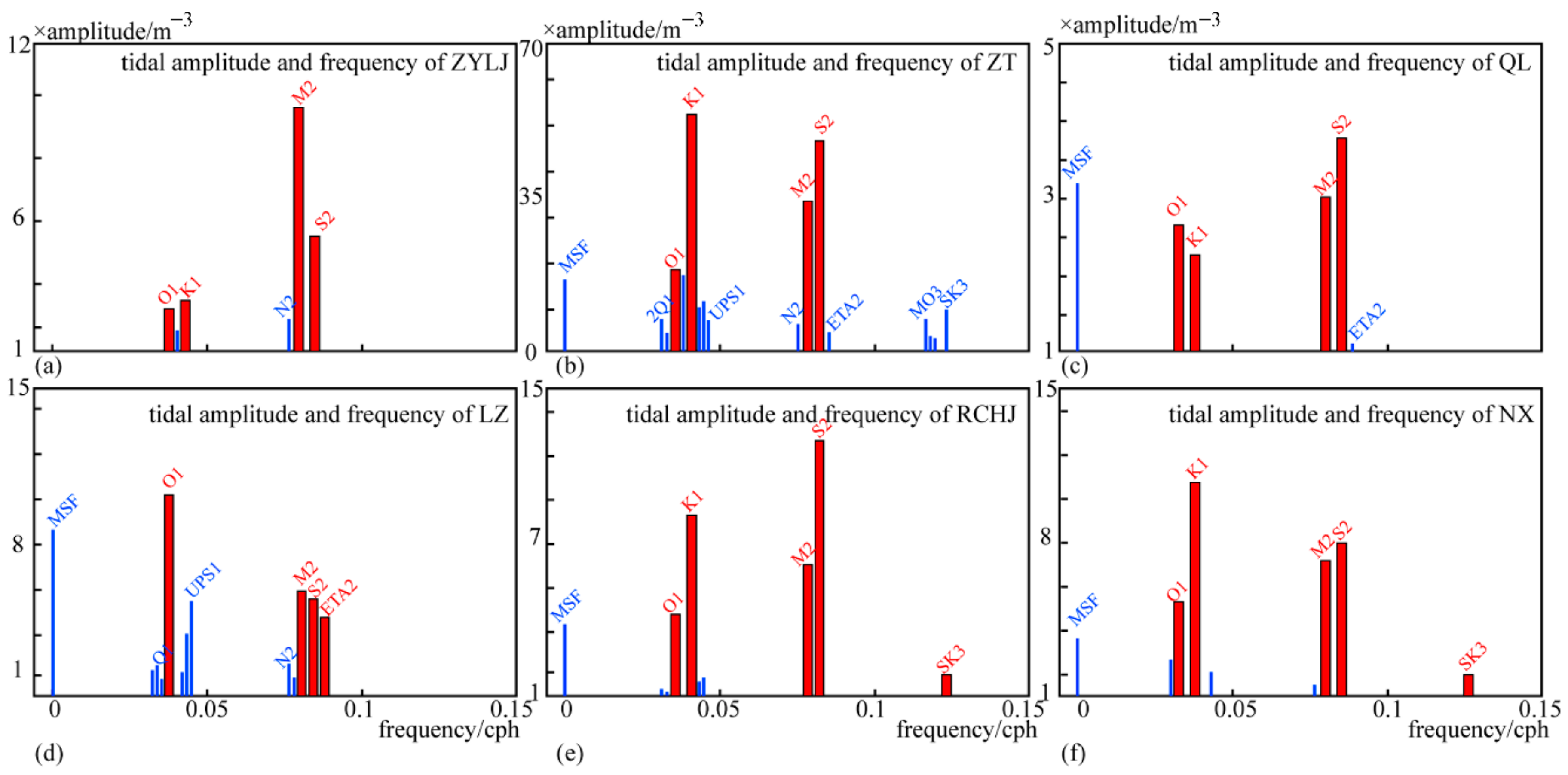
3. Data Preparation
- To remove data extrema from the water level sequences. For the rock media, the magnitude of increased volume result from the cracks, in terms of the studies of Brace et al. [25], is no more than 2.0 times the elastic volume variations. Thus, the data points whose values exceed twice the average amplitude of the water level sequence are removed.
- To linearly interpolate values to the missing data in the water level sequences.
- To perform 12.4~26 h (mainly including the M2 and O1 tidal data) Butterworth bandpass filtering on the data to remove signals unrelated to the tidal process.
4. Application to Seismic Data
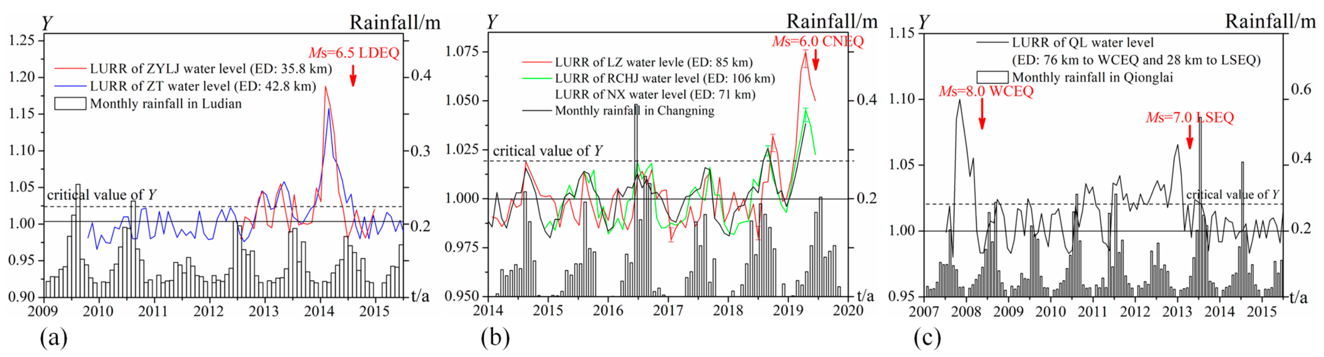
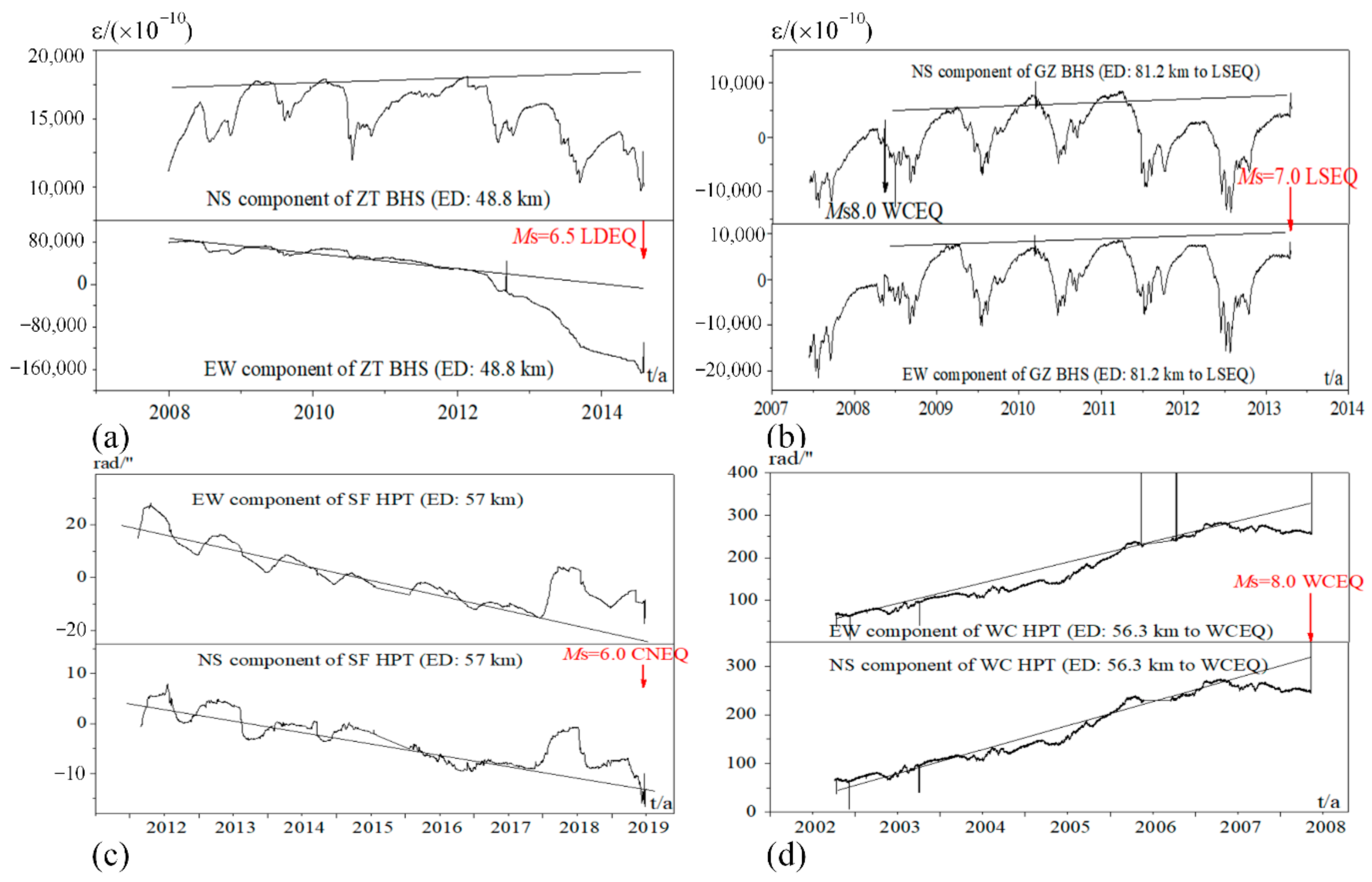
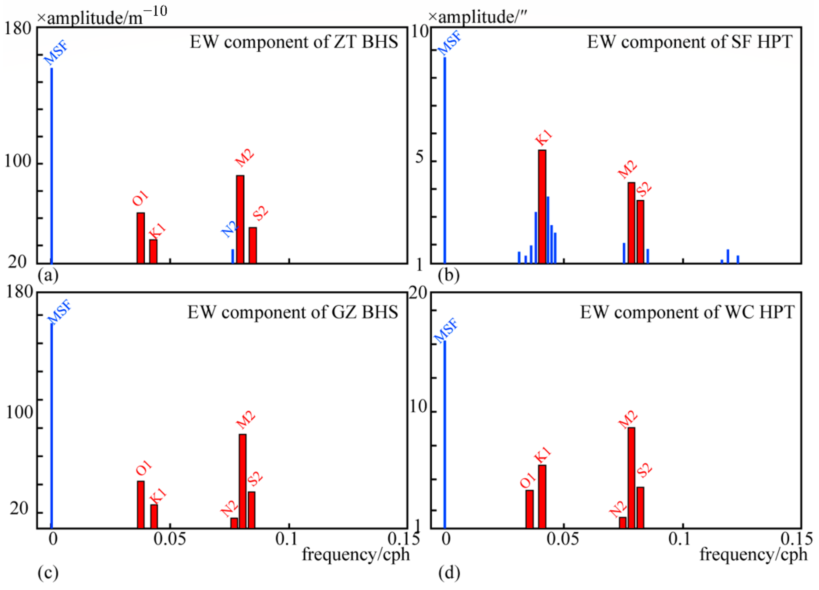
5. Results and Interpretation
6. Discussion
7. Conclusions
Author Contributions
Funding
Institutional Review Board Statement
Informed Consent Statement
Data Availability Statement
Acknowledgments
Conflicts of Interest
References
- Koizumi, N.; Kitagawa, Y.; Matsumoto, N.; Takahashi, M.; Sato, T.; Kamigaichi, O.; Nakamura, K. Pre-seismic groundwater level changes induced by crustal deformations related to earthquake swarms off the east coast of Izu Peninsula, Japan. Geophys. Res. Lett. 2004, 31, L10606. [Google Scholar] [CrossRef]
- Wang, C.; Manga, M. Earthquakes and Water; Springer: Berlin/Heidelberg, Germany, 2010. [Google Scholar]
- Yuce, G.; Ugurluoglu, D.Y.; Adar, N.; Yalcin, T.; Yaltirak, C.; Streil, T.; Oeser, V. Monitoring of earthquake precursors by multi-parameter stations in Eskisehir region (Turkey). Appl. Geochem. 2010, 25, 572–580. [Google Scholar] [CrossRef]
- Roeloffs, E.A. Persistent water level changes in a well near Parkfield, California, due to local and distant earthquakes. J. Geophys. Res. 1998, 103, 869–889. [Google Scholar] [CrossRef]
- King, C.Y.; Azuma, S.; Igarashi, G.; Ohno, M.; Saito, H.; Wakita, H. Earthquake related water level changes at 16 closely clustered wells in Tono, central Japan. J. Geophys. Res. 1999, 104, 13073–13082. [Google Scholar] [CrossRef] [Green Version]
- Brodsky, E.E.; Roeloffs, E.; Woodcock, D.; Gall, I.; Manga, M. A mechanism for sustained groundwater pressure changes induced by distant earthquakes. J. Geophys. Res. 2003, 108, 2390. [Google Scholar] [CrossRef] [Green Version]
- Montgomery, D.R.; Manga, M. Streamflow and water well response to earthquake. Science 2003, 300, 2047–2049. [Google Scholar] [CrossRef] [PubMed] [Green Version]
- Cicerone, R.D.; Ebel, J.E.; Britton, J. A systematic compilation of earthquake precursors. Tectonophysics 2009, 476, 371–396. [Google Scholar] [CrossRef]
- Roeloffs, E.A. Hydrologic precursors to earthquakes: A review. Pure Appl. Geophys. 1988, 126, 177–209. [Google Scholar] [CrossRef]
- Kissin, I.G.; Belikov, V.M.; Ishankuliev, G.A. Short-term groundwater level variations in a seismic region as an indicator of the geodynamic regime. Tectonophysics 1996, 265, 313–326. [Google Scholar] [CrossRef]
- King, C.Y.; Azuma, S.; Ohno, M.; Wakita, H. In search of earthquake precursors in the water-level data of 16 closely clustered wells at Tono, Japan. Geophys. J. Int. 2008, 143, 469–477. [Google Scholar] [CrossRef] [Green Version]
- Liu, Y.W.; Chen, T.; Xie, F.R.; Du, F.; Yang, D.X.; Zhang, L.; Xu, L.Q. Analysis of fluid induced aftershocks following the 2008 WenchuanMs8.0 earthquake. Tectonophysics 2014, 149, 619–620. [Google Scholar]
- Skelton, A.; Andrén, M.; Kristmannsdóttir, H.; Stockmann, G.; Mörth, C.M.; Sveinbjörnsdóttir, Á. Changes in groundwater chemistry before two consecutive earthquakes in Iceland. Nat. Geosci. 2014, 7, 752–756. [Google Scholar] [CrossRef] [Green Version]
- Ma, Z.; Yu, C.; Zhang, X.T.; Yu, H.Z. Evolutions of LURR Anomaly based on Seismicity and Groundwater Level Data before the 17 June 2019 M6.0 Changning Earthquake. Earthq. Res. China 2020, 36, 550–560, (In Chinese with English abstract). [Google Scholar]
- Yin, X.C.; Chen, X.Z.; Song, Z.P.; Yin, C. A New Approach to Earthquake Prediction–The Load/Unload Response Ratio (LURR) Theory. Pure Appl. Geophys. 1995, 145, 701–715. [Google Scholar] [CrossRef]
- Zhang, Y.X.; Yin, X.C.; Peng, K.Y. Spatial and Temporal Variation of LURR and its Implication for the Tendency of Earthquake Occurrence in Southern California. Pure Appl. Geophys. 2004, 161, 2359–2367. [Google Scholar] [CrossRef] [Green Version]
- Yu, H.Z.; Zhou, F.R.; Cheng, J.; Wan, Y.G. The sensitivity of loa/unload response ratio and critical region selection before large earthquakes. Pure Appl. Geophys. 2015, 172, 173–183. [Google Scholar] [CrossRef]
- Yu, H.Z.; Shen, Z.K.; Wan, Y.G.; Zhu, Q.Y.; Yin, X.C. Increasing critical sensitivity of the Load/Unload Response Ratio before large earthquakes with identified stress accumulation pattern. Tectonophysics 2006, 428, 87–94. [Google Scholar] [CrossRef]
- Yu, H.Z.; Zhu, Q.Y. A Probabilistic Approach for Earthquake Potential Evaluation Based on the Load/Unload Response Ratio Method. Concurr. Comput. Pract. Exp. 2010, 22, 1520–1533. [Google Scholar] [CrossRef]
- Liu, Y.; Yin, X.C. A dimensional analysis method for improved load-unload response ratio. Pure Appl. Geophys. 2018, 175, 633–645. [Google Scholar] [CrossRef] [Green Version]
- Jaeger, J.C.; Cook, N.G.W. Fundamentals of Rock Mechanics; Chapman and Hall: London, UK, 1976; pp. 78–99. [Google Scholar]
- Igarashi, G.; Wakita, H. Tidal responses and earthquake-related changes in the water level of deep wells. J. Geophys. Res. 1991, 96, 4269–4278. [Google Scholar] [CrossRef]
- Elkhoury, J.E.; Brodsky, E.E.; Agnew, D.C. Seismic waves increase permeability. Nature 2006, 441, 1135–1138. [Google Scholar] [CrossRef] [PubMed]
- Zhang, H.; Shi, Z.; Wang, G.; Sun, X.; Yan, R.; Liu, C. Large earthquake reshapes the groundwater flow system: Insight from the water-level response to earth tides and atmospheric pressure in a deep well. Water Resour. Res. 2019, 55, 4207–4219. [Google Scholar] [CrossRef] [Green Version]
- Vittecoq, B.; Fortin, J.; Maury, J.; Violette, S. Earthquakes and extreme rainfall induce long term permeability enhancement of volcanic island hydrogeological systems. Sci. Rep. 2020, 10, 20231. [Google Scholar] [CrossRef] [PubMed]
- Muir-Wood, R.; King, G. Hydrological signatures associated with earthquakes train. J. Geophys. Res. 1993, 98, 22035–22068. [Google Scholar] [CrossRef]
- Gudmundsson, A.; Berg, S.; LysloK, B. Fracture networks and fluid transport in active fault zone. J. Struct. Geol. 2001, 23, 343–353. [Google Scholar] [CrossRef]
- Brace, W.B.; Paulding, J.R.; Scholz, C. Dilatancy in the fracture of crystalline rocks. J. Geophys. Res. 1966, 71, 3939–3953. [Google Scholar] [CrossRef]
- Yin, X.C.; Zhang, L.P.; Zhang, Y.X.; Peng, K.Y.; Wang, H.T.; Song, Z.P.; Yu, H.Z. The newest developments of load-unload response ratio (LURR). Pure Appl. Geophys. 2008, 165, 711–722. [Google Scholar] [CrossRef] [Green Version]
- Scholz, C.H.; Sykes, L.R.; Aggarwal, Y.P. Earthquake prediction: A physical basis. Science 1973, 181, 803–809. [Google Scholar] [CrossRef]
- Li, C.; Nordlund, E. Experimental verification of the Kaiser effect in rocks. Rock Mech. Rock Eng. 1993, 26, 333–351. [Google Scholar] [CrossRef]
- Kurita, K.; Fujii, N. Stress memory of crystalline rocks in acoustic emission. Geophys. Res. Lett. 1979, 6, 9–12. [Google Scholar] [CrossRef]
- Byerlee, J.D. Friction of rocks. Pure Appl. Geophys. 1978, 116, 615–626. [Google Scholar] [CrossRef]
- Yin, X.C.; Wang, Y.C.; Peng, K.; Bai, Y.L.; Wang, H.; Yin, X.F. Development of a New Approach to Earthquake Prediction: Load/Unload Response Ratio (LURR) Theory. Pure Appl. Geophys. 2000, 157, 2365–2383. [Google Scholar] [CrossRef] [Green Version]
- Harris, R.A. Earthquake stress trigger, stress shadows, and seismic hazard. J. Geophys. Res. 1998, 103, 24347–24358. [Google Scholar] [CrossRef]
- Zoback, M.D.; Zoback, M.L.; Mount, V.; Wentworth, C.M. New evidence on state of stress of the San Andreas fault system. Science 1987, 238, 1105–1111. [Google Scholar] [CrossRef]
- Wilhelm, H.; Zürn, W.; Wenzel, H.G. (Eds.) Tidal Triggering of Earthquakes and Volcanic Events; Tidal Phenomena; Springer: Berlin/Heidelberg, Germany, 1997; pp. 293–309. [Google Scholar]
- Hardebeck, J.L.; Hauksson, E. Crustal stress field in southern California and its implications for fault mechanics. J. Geophys. Res. 2001, 106, 21859–21882. [Google Scholar] [CrossRef]
- Vidali, J.E.; Agnew, D.C.; Johnston, M.J.S.; Oppenheimer, D.H. Absence of earthquake correlation with earth tides: An indication of high preseismic fault stress rate. J. Geophys. Res. 1998, 103, 24567–24572. [Google Scholar] [CrossRef]
- Yu, H.Z.; Yu, C.; Ma, Z.; Zhang, X.T.; Zhang, H.; Yao, Q.; Zhu, Q.Y. Temporal and spatial evolution of load/unload response ratio before the M7.0 Jiuzhaigou earthquake occurred on 8 August 2017 in Sichuan Province. Pure Appl. Geophys. 2020, 177, 321–331. [Google Scholar] [CrossRef]
- Dziewonski, A.M.; Anderson, D.L. Preliminary reference earth model. Phys. Earth Planet. Inter. 1981, 25, 297–356. [Google Scholar] [CrossRef]
- Melchior, P. The Tide of the Planet Earth; Pergamon Press: New York, NY, USA, 1978. [Google Scholar]
- Pawlowicz, R.; Beardsley, B.; Lentz, S. Classical tidal harmonic analysis including error estimates in MATLAB using T_TIDE. Comput. Geosci. 2002, 28, 929–937. [Google Scholar] [CrossRef]
- Zhao, Y.C.; Liu, X.W. A data processing method for eliminating annual variation. North China Earthq. Sci. 1984, 2, 65–69. [Google Scholar]
- Pei, S.P.; Niu, F.L.; Ben-zion, Y.; Sun, Q.; Liu, Y.B.; Xue, X.T.; Su, J.R.; Shao, Z.G. Seismic velocity reduction and accelerated recovery due to earthquakes on the Longmenshan fault. Nat. Geosci. 2019, 12, 680. [Google Scholar] [CrossRef]
- Wawersik, W.R.; Brace, W.F. Post-failure behavior of a granite and diabase. Rock Mech. 1971, 3, 61–85. [Google Scholar] [CrossRef]
- Hauksson, E.L.; Jones, M.; Hutton, K. The 1999 Mw7.1 Hector Mine, California, earthquake sequence: Complex conjugate strike-slip faulting. Bull. Seismol. Soc. Am. 2002, 92, 1154–1170. [Google Scholar] [CrossRef] [Green Version]


| Event | Well Name | Epicentral Distance (km) | Well Location (Lat/Lon) | Start Time | Depth (m) | Sampling Frequency |
|---|---|---|---|---|---|---|
| LDEQ | ZYLJ | 35.8 | 27.38/103.58 | 20120524 | 114 | 1-h |
| ZT | 42.8 | 27.45/103.58 | 20100101 | 350 | 1-h | |
| CNEQ | LZ | 85 | 27.38/103.58 | 20130524 | 300 | 1-h |
| RCHJ | 106 | 27.45/103.58 | 20140101 | 251 | 1-h | |
| NX | 71 | 28.98/104.93 | 20120601 | 105 | 1-h | |
| WCEQ | QL | 76 | 30.32/103.28 | 20070630 | 175 | 1-h |
| No. | Name of Station | Observation Type | Instrument | Resolution |
|---|---|---|---|---|
| 1 | Zhaoyangleju | Groundwater level | TDL-15 | 0.001 m |
| 2 | Zhaotong | Groundwater level | LN-3A | 0.001 m |
| 3 | Luzhou | Groundwater level | SWY-Ⅱ | 0.001 m |
| 4 | Rongchanghuajiang | Groundwater level | SWY-Ⅱ | 0.001 m |
| 5 | Nanxi | Groundwater level | LN-3A | 0.001 m |
| 6 | Qionglai | Groundwater level | SWY-Ⅱ | 0.001 m |
| 7 | Shuifu | Horizontal pendulum tiltmeter | SSQ-2 | 0.0005″ |
| 8 | Zhaotong | borehole strain | RZB-2 | 5 × 10⁻⁹ |
| 9 | Wenchuan | Horizontal pendulum tiltmeter | JB-1 | 0.002″ |
| 10 | Guza | borehole strain | YRY-4 | 1 × 10⁻¹⁰ |
Publisher’s Note: MDPI stays neutral with regard to jurisdictional claims in published maps and institutional affiliations. |
© 2021 by the authors. Licensee MDPI, Basel, Switzerland. This article is an open access article distributed under the terms and conditions of the Creative Commons Attribution (CC BY) license (https://creativecommons.org/licenses/by/4.0/).
Share and Cite
Yu, H.; Yu, C.; Ma, Y.; Zhao, B.; Yue, C.; Gao, R.; Chang, Y. Determining Stress State of Source Media with Identified Difference between Groundwater Level during Loading and Unloading Induced by Earth Tides. Water 2021, 13, 2843. https://doi.org/10.3390/w13202843
Yu H, Yu C, Ma Y, Zhao B, Yue C, Gao R, Chang Y. Determining Stress State of Source Media with Identified Difference between Groundwater Level during Loading and Unloading Induced by Earth Tides. Water. 2021; 13(20):2843. https://doi.org/10.3390/w13202843
Chicago/Turabian StyleYu, Huaizhong, Chen Yu, Yuchuan Ma, Binbin Zhao, Chong Yue, Rong Gao, and Yulong Chang. 2021. "Determining Stress State of Source Media with Identified Difference between Groundwater Level during Loading and Unloading Induced by Earth Tides" Water 13, no. 20: 2843. https://doi.org/10.3390/w13202843