Inland Reservoir Water Quality Inversion and Eutrophication Evaluation Using BP Neural Network and Remote Sensing Imagery: A Case Study of Dashahe Reservoir

Abstract

In this study, an inland reservoir water quality parameters’ inversion model was developed using a back propagation (BP) neural network to conduct reservoir eutrophication evaluation, according to multi-temporal remote sensing images and field observations. The inversion model based on the BP neural network (the BP inversion model) was applied to a large inland reservoir in Jiangmen city, South China, according to the field observations of five water quality parameters, namely, Chlorophyl-a (Chl-a), Secchi Depth (SD), total phosphorus (TP), total nitrogen (TN), and Permanganate of Chemical Oxygen Demand (CODMn), and twelve periods of Landsat8 satellite remote sensing images. The reservoir eutrophication was evaluated. The accuracy of the BP inversion model for each water parameter was compared with that of the linear inversion model, and the BP inversion models of two parameters (i.e., Chl-a and CODMn) with larger fluctuation range were superior to the two multiple linear inversion models due to the ability of improving the generalization of the BP neural network. The Dashahe Reservoir was basically in the state of mesotrophication and light eutrophication. The area of light eutrophication accounted for larger proportions in spring and autumn, and the reservoir inflow was the main source of nutrient salts.

1. Introduction

Reservoirs play an important role in the supply of inland fresh water resources [1,2]. However, in recent decades, as a result of the growing population and the rapidly developing economy, the problem of reservoir eutrophication has become increasingly serious, resulting in the reduction in biodiversity and degradation of freshwater, and posing a significant threat to water supplies [3,4]. It thus is necessary to strengthen the monitoring and supervision of water quality conditions in reservoirs [5,6]. Traditional water quality monitoring at cross sections is difficult and time and labor consuming, and it is hard to quickly reflect the overall water quality of reservoirs [7]. By comparison, remote sensing technology can be used to rapidly and continuously present the water quality condition of the entire water body in a global spatial and multi-temporal manner, with the characteristics of a wide range of monitoring, low cost, and long-term dynamic monitoring [8,9]. Therefore, when applied to the monitoring of reservoir water quality parameters, this approach can fully and effectively reflect reservoir water quality conditions combined with field observations.

Remote sensing techniques, which were initially used for the analysis of ocean color and surface temperature in the 1970s [10,11], have long been applied to water quality monitoring [12,13]. A large number of scholars have completely and intensively explored the hydrological, biological, and chemical characteristics of water. Thus, it is practicable for remote sensing techniques to be used in the field of water quality monitoring and assessment [14,15,16,17]. Because remote sensing techniques enable effective and efficient monitoring of waterbodies at a large spatiotemporal scale, many researchers have obtained correlations between remote sensing data and water quality parameters using three main types of model, namely, empirical, semi-analytical, or machine learning models [18,19,20]. Empirical models consist of a standard linear regression between spectral bands or band ratio values from remote sensing and in situ water quality measurements. This is a simple and minimal computational approach at a local scale, but suffers from a shortage of optically non-homogenous waterbodies at a large spatiotemporal scale [21,22,23]. In contrast, the semi-analytical model combines a physics-based approach with parameters relating to water’s inherent optical properties, and then incorporates in situ measurements to parameterize the inverse equation to estimate water quality parameters [19]. Some scholars attained sound estimates of multiple water quality parameters based on the semi-analytical model at large spatiotemporal scales [24,25]. However, the semi-analytical model requires a large amount of in situ data for model validation [26]. In addition, it is challenging to obtain several important water quality parameters, such as pH, ammonia nitrogen (NH₃-N), and dissolved phosphorus (DP), in water quality monitoring and assessment using remote sensing techniques due to the weak optical characteristics and low signal noise ratio [27]. Water bodies can be divided into Case-1 water and Case-2 water according to their different optical properties [1,2]. The optical properties of Case-1 water are mainly determined by phytoplankton and associated organisms, whereas the optical properties of Case-2 water are mainly determined by the suspended matter and colored dissolved organic matter (CDOM). Case-1 water (stratified shelf seas and the deep ocean) is colored by biogenic materials alone [28]. Case-2 water is usually located near shores, estuaries, and other places which are seriously affected by terrigenous matter discharge [29]. Compared with Case-1 water, Case-2 water is more closely related to humans and is most strongly affected by human activities. Because inland Case-2 waters are seriously impacted by humans, the optical properties are complex and changeable [30]. Thus, the linear model incompletely represents the relationship between the complex water constituents and remote sensing data [31]. Furthermore, publications have mainly focused on eutrophic inversion of a single parameter rather than multiple water parameters [32,33,34].

In recent years, as a result of the development of machine learning in the field of remote sensing, intelligent algorithms have been introduced to address the complex linear or non-linear relationships between remote sensing data and multiple water quality parameters [35,36]. Moreover, some water parameters, such as phosphorus, COD, or BOD, are not optically active and therefore do not modify the water response to the electromagnetic spectrum. In addition, their relationships with the spectral characteristics of images are still poorly understood, and the study of these parameters using machine learning is therefore valuable [27]. Machine learning algorithms, which mainly include artificial neural networks, genetic algorithms, support vector machines, and random forest, are relatively promising in improving the accuracy of water quality monitoring at large spatiotemporal scales [37,38,39,40]. Unlike empirical and semi-analytical models, the machine learning algorithms can reduce overall error and obtain the best fitting model with iterative learning. Furthermore, the machine learning algorithms can be normally operated under different assumptions during their training stage when in situ measurements are lacking [41,42]. As a result, the integration of the remote sensing technique, auxiliary in situ measurements, and extensive computer modelling capacity has a promising future in water quality monitoring. The back propagation (BP) neural network, proposed by a team led by Rumelhart, D.E. and McCelland, J.L. [43] in 1987, is one of the most widely used neural network models, and is a multilayer feedforward network trained by the error back propagation algorithm. The development of the BP neural network is relatively mature and the model is easy to implement compared to the numerous machine learning algorithms [44,45]. BP neural networks have been shown to be capable of simulating complex nonlinear relationships with a hyperbolic tangent function hidden layer and a linear output layer [46]. Therefore, they have been increasingly adopted in the inversion of water quality parameters for inland Case-2 waters, combined with the remote sensing technique [32,33,34,47,48]. However, previous research has mainly focused on eutrophic inversion of a single parameter rather than multiple parameters. For example, total phosphorus (TP) is an essential element of algae growth and also an important factor in eutrophication [48]; chemical oxygen demand (COD) is the quantity of matter, particularly organic contamination, that needs to be oxidized in water, and is measured with a chemical method [27]; and total nitrogen (TN) is one of the major factors that probably results in eutrophication and algal blooms in rivers, lakes, and reservoirs [49]. Analyses of these water quality parameters are essential for eutrophication evaluation. For the inland Case-2 waters, such as reservoirs, it is necessary to incorporate multiple water quality parameters for eutrophication evaluation. This can be done by integrating remote sensing technology and a BP neural network in an inversion model, which has been rarely considered in the existing literature.

Given the above, the objective of this study was to develop an inversion model of multi-temporal remote sensing image data and reservoir water quality parameters using a BP neural network, with the main aims of monitoring multiple water quality parameters of inland Case-2 waters and evaluating reservoir eutrophication. The current study took the Dashahe Reservoir, a typical inland Case-2 water body located in the coastal area of Guangdong province, South China, as an example. An inversion model based on a BP neural network (the BP inversion model) was built based on Landsat8 satellite remote sensing images and field observations of five water quality parameters (i.e., Chl-a, SD, TP, TN, and CODMn). The Landsat8 satellite is equipped with two main sensors [50]: the Operational Land Image (OLI) and Thermal Infrared Sensor (TIRS). The OLI consists of nine wavebands, covering wavelengths from infrared to visible light [51]; the spatial resolution of the multi-temporal image is 30 m, and the spatial resolution of the panchromatic band is 15 m. The TIRS includes two separate thermal infrared bands with a resolution of 100 m, which can be used to monitor surface temperature [52]. In addition, the eutrophication degree of the reservoir was evaluated, according to the inversion value of the five water quality parameters. This study can provide technical support for water quality monitoring and reservoir eutrophication evaluation at an extensive scale and in continuous space.

2. Materials and Methods

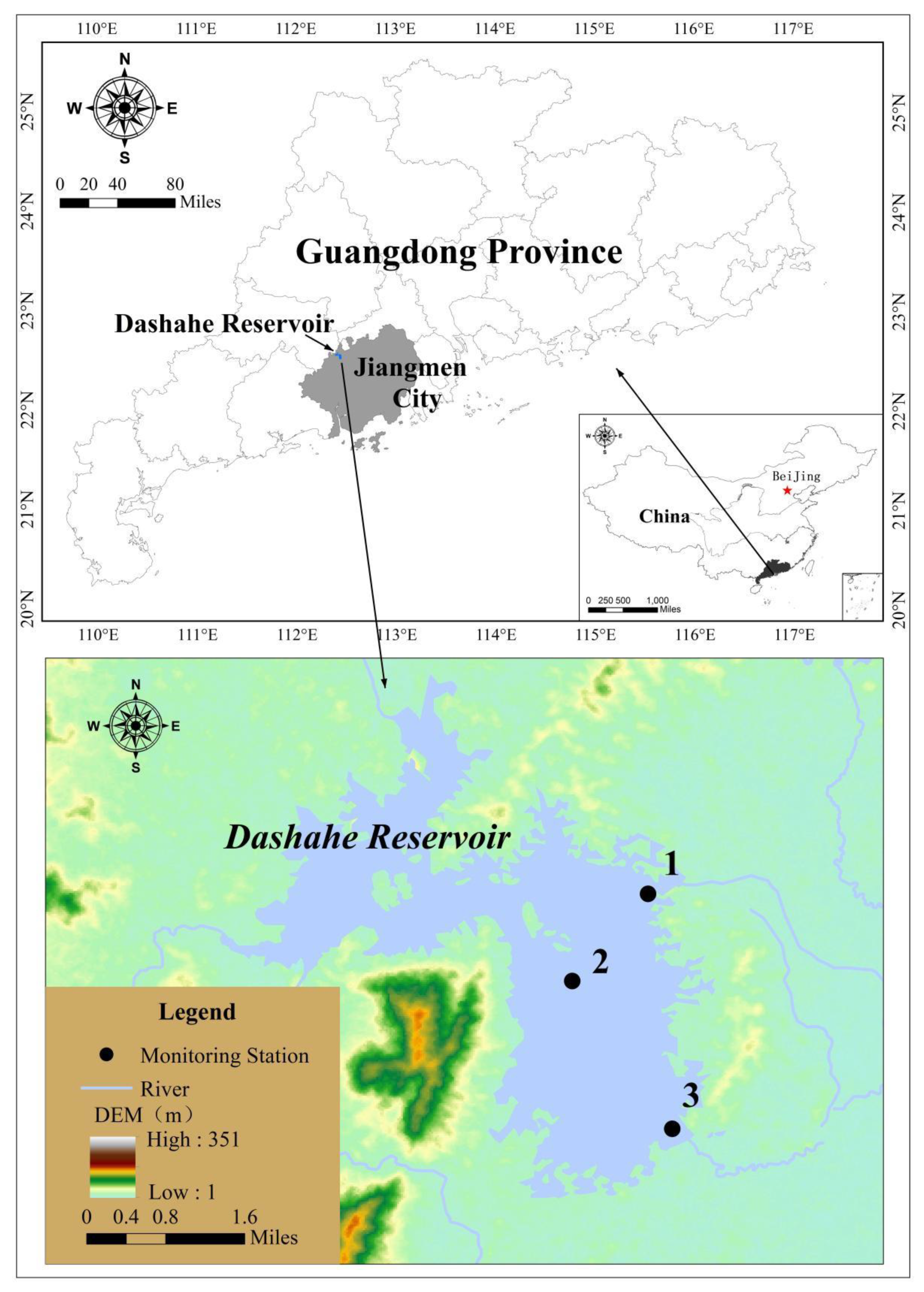
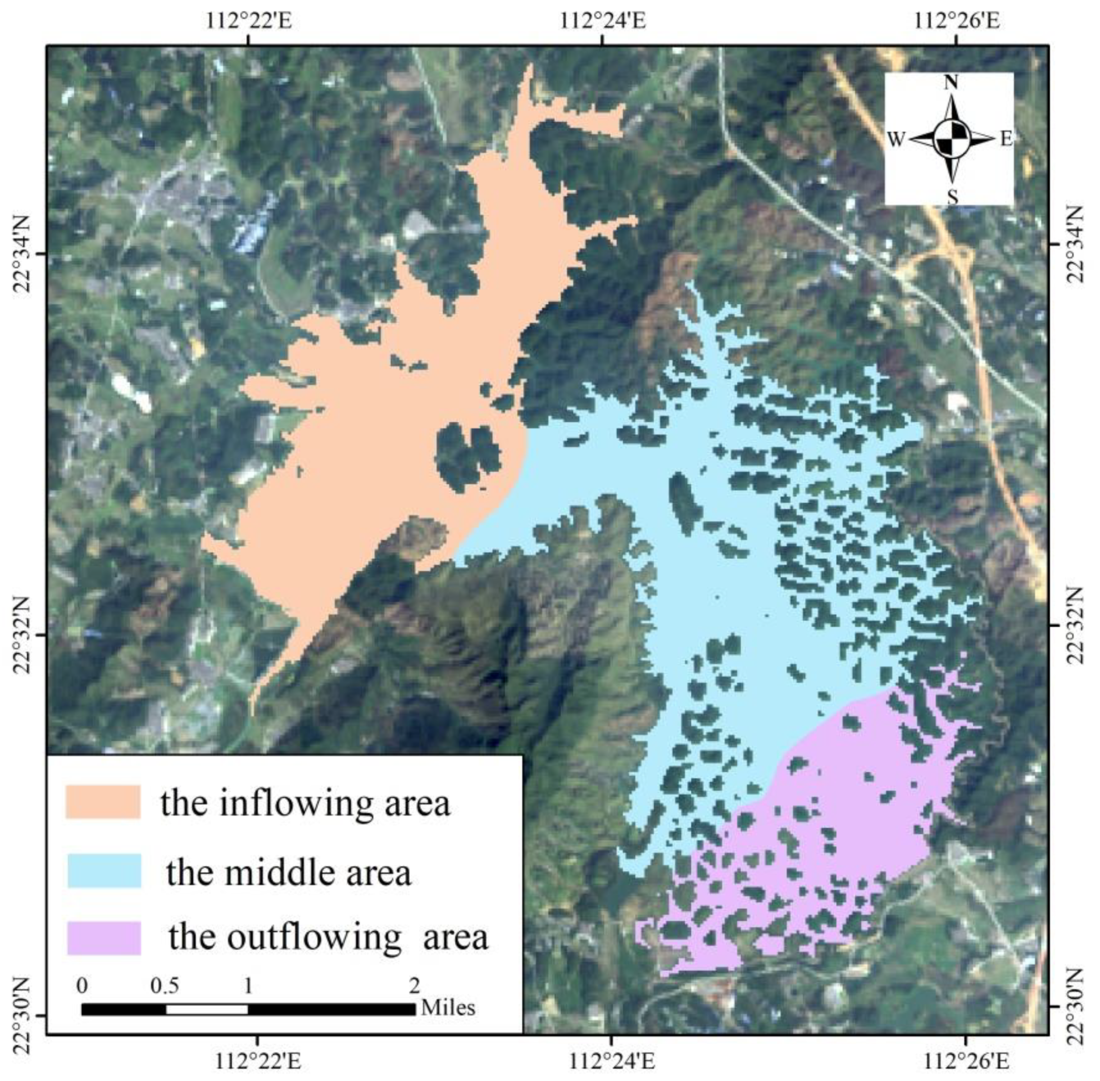
2.1. Study Area

Dashahe Reservoir is located to the northwest of Jiangmen city, Guangdong province, South China, and has a catchment area of 217 km² and water area of 16.3 km² (Figure 1). The reservoir has 152 uninhabited islands covered in green vegetation and three main inflow tributaries (i.e., Dasha River, Wojiang River, and Fushi River). The watershed has a subtropical ocean monsoon climate with a yearly average air temperature of approximately 22 °C, precipitation of nearly 2000 mm, and surface water resources volume of 10⁴ m³ [53]. Summer rainy events (May to July) contribute more than 50% of the total precipitation because of typhoons and tropical depressions [54]. As the largest reservoir in Kaiping city, Dashahe Reservoir is the main drinking water source and plays an important role in the city’s water supply, flood control, power generation, and fish breeding. The water quality of the reservoir reached the surface water Class II water standard in 2017. The reservoir has experienced blooms of cyanobacteria due to a large amount of agricultural wastewater and municipal sewage discharged into the tributaries, which may cause water and public health risks due to waterborne pathogens [53,55].

2.2. Materials

2.2.1. Field Observations of Water Quality Parameters

Since 2003, monthly monitoring of water quality parameters has been conducted in Dashahe Reservoir; the water quality parameters include Chl-a concentration, CODMn, TN, TP, SD, temperature, and heavy metal content. Three monitoring stations are evenly distributed in the reservoir (Figure 1).

The samples were collected by the Hydrology Sub-bureau of Jiangmen city, which is responsible for monitoring the hydrology and water quality of rivers, lakes, and reservoirs in Jiangmen. The determination of total phosphorus, total nitrogen, chlorophyll a, and the permanganate index was undertaken, respectively, according to Water quality-Determination of total phosphorus-Ammonium moly date spectrophotometric method (GB 11893-89), Water quality-Determination of total nitrogen-Alkaline potassium persulfate digestion-UV spectrophotometric method (GB 11894-89), Water quality-Determination of chlorophyll a-Spectrophotometric method (HJ 897-2017), and Water quality-Determination of permanganate index (GB11892-1989). In the current study, the water measurements were collected at the surface.

2.2.2. Satellite Image Data

The Landsat8 satellite was launched on 11 February 2013, and has an altitude of 705 km and a period of 16 days around the Earth. It can provide seasonal coverage of the global landmass at a spatial resolution of 30 m (visible, NIR, SWIR); 100 m (thermal); and 15 m (panchromatic). The visible bands’ data were applied to this study.

Thirty-five original Landsat8 satellite images (WRS_PATH = 123, WRS_ROW = 44) that meet the requirement of simultaneous observation on sky–ground at Dashahe Reservoir were obtained from National Science & Technology Infrastructure (http://www.nsdata.cn/, accessed on 1 March 2019). In addition, 12 images with a cloudless sky over Dashahe Reservoir (

Table 1. The date of water measurements and the acquisition date of the Landsat 8 images.

No.	Date of Water Measurements	Date of the Landsat 8 Images
1	9 October 2013	3 October 2013
2	9 December 2013	6 December 2013
3	5 August 2014	3 August 2014
4	5 August 2014	3 August 2014
5	2 December 2014	9 December 2014
6	8 April 2015	16 April 2015
7	1 March 2016	1 March 2016
8	6 December 2016	28 November 2016
9	6 September 2017	12 September 2017
10	7 November 2017	30 October 2017
11	6 December 2017	1 December 2017
12	2 February 2018	3 February 2018

), having high definition and fine visibility, were identified from all the images according to the image characteristics of cloud coverage, visibility, etc.

2.3. Methods

2.3.1. Radiation Calibration

The Digital Number (DN), an integer value without a unit, is the brightness value of each pixel in the remote sensing image, and records gray information of the ground object carried by the pixel. Its value is related to the radiative resolution of the sensor, ground object emittance, atmospheric transmittance, and scattering rate. The purpose of radiation calibration is to eliminate the sensor error and identify the accurate radiation value at the sensor entrance via converting the original DN into the surface reflectance of the outer atmosphere [56]. The radiation calibration was as follows:

L = DN × Gain + Offset

(1)

where L is the brightness of radiation, and Gain represents absolute gain for the radiation calibration coefficient. The Environment for Visualizing Images (ENVI) (Ver.5.3.1, Harris Geospatial Solutions, Inc. VBroomfield, CO, USA) software can automatically acquire these parameters from an image file when choosing the type of sensor for radiometric calibration. In the current study, ENVI software was used for radiation calibration, Fast Line-of-sight Atmospheric Analysis of Spectral Hypercubes (FLAASH,) atmospheric correction, and water body extraction.

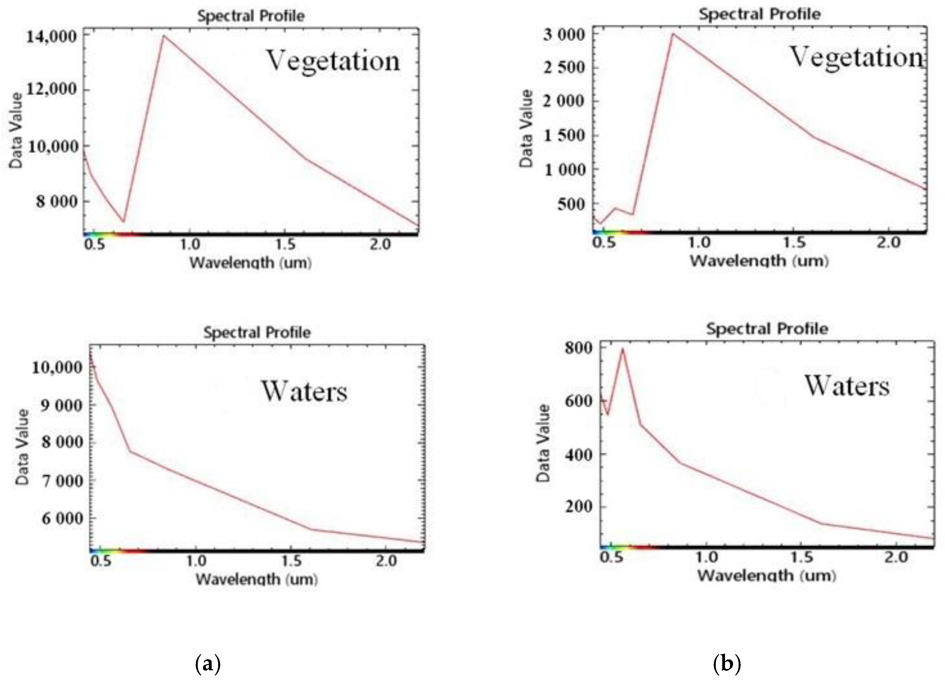
2.3.2. FLAASH Atmospheric Correction

Satellites are affected by cloud ions, atmospheric molecules and aerosols, etc., resulting in low accuracy of remote sensing analysis. This is because the images contain some redundant target information. It is necessary to conduct atmospheric correction, namely, by translating the radiation brightness or surface reflectance into the real reflectance of the ground and eliminating the error caused by atmospheric scattering, absorption, and reflection. The FLAASH, a kind of code with MODTRAN4+ as the transmission model, can not only adjust the classification images containing opaque layers and cirrus clouds, but also adjust spectrum smoothing caused by human factors, and quickly rectify and analyze the hyper-spectral and multi-temporal images of SPOC and Landsat [57]. FLAASH was originally applied to land atmospheric correction, and it now has been used in water color remote sensing with OLI data, achieving satisfactory results [51,58,59,60]. Moreover, FLAASH can achieve high accuracy via a simple operation, and does not require auxiliary information on field measurements [61].

As shown in Figure 2, the spectral curves of vegetation and waters after atmospheric correction are close to the standard spectral curves. There are two obvious valleys of chlorophyll reflection in the visible band and one obvious reflection peak in the near-infrared band. The reflectivity of clean water in each waveband gradually decreases. Dashahe Reservoir belongs to the inland Case-2 waters with complex water composition. Field sampling found that the water of Dashahe Reservoir contains a large number of algae, all of which contain chlorophyll. When the density of algae in the water body is too high, the spectral curve has a peak in the green light band. FLAASH has been previously implemented for the atmospheric correction of high-resolution imagery and has achieved excellent results [51,62]. The error caused by atmospheric absorption and scattering can be effectively eliminated after atmospheric correction using FLAASH. As a result of the improvement in image quality, the corrected image accurately reflects the real characteristics of the surface spectrum.

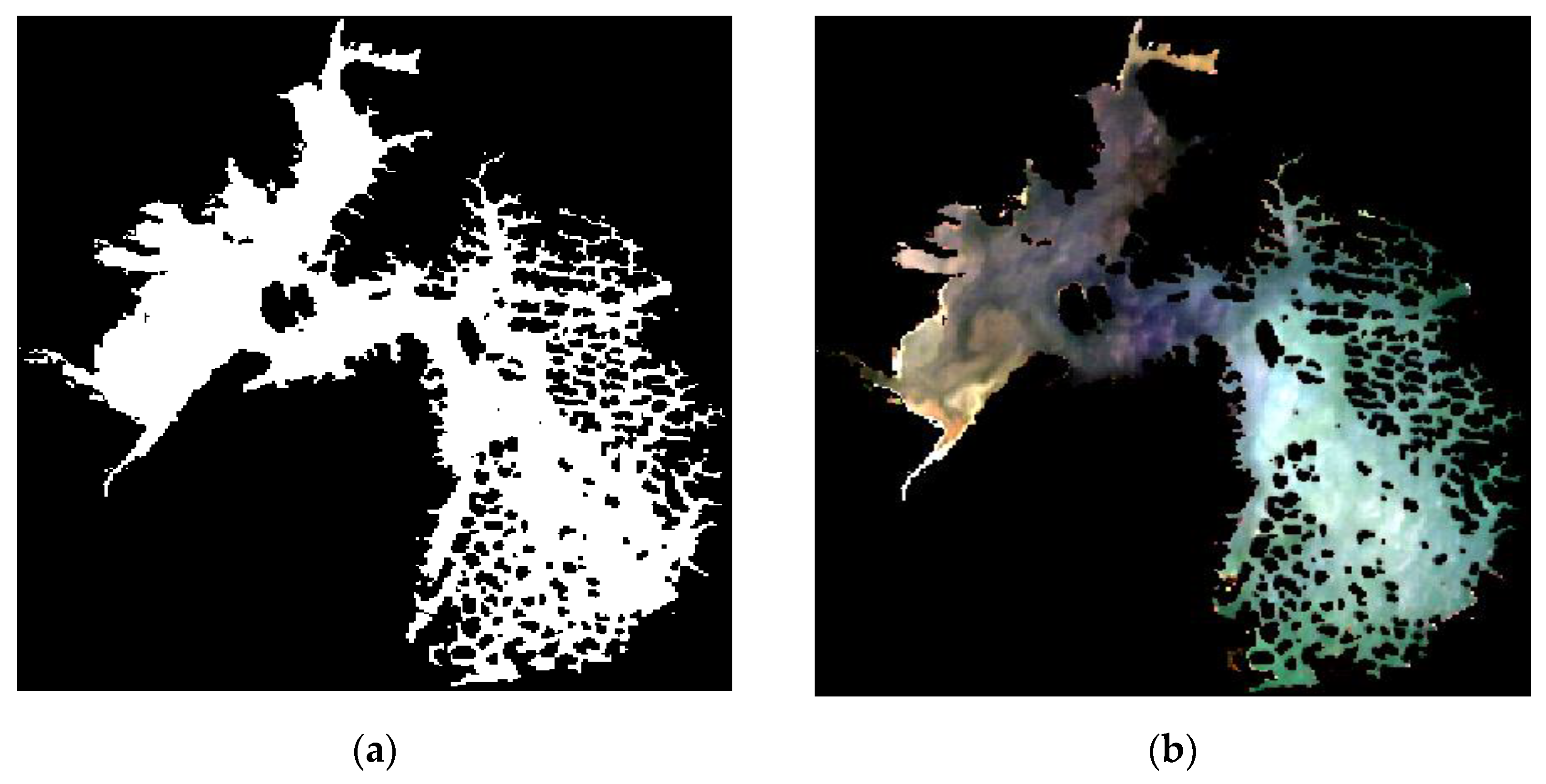
2.3.3. Water Body Extraction

The accuracy of the inversion results of the reservoir can be easily disturbed due to various scales of land areas covered with vegetation on their surface. Therefore, it is necessary to extract the water body from Dashahe Reservoir and remove the land located in the water area.

The ratio of wavebands can be used to reduce the impact of terrain slope, slope direction, and shadow, and therefore improve the accuracy of water body identification. The normalized difference water index (NDWI) model was built to filter vegetation information and enhance water information as much as possible, according to the green and near-infrared bands [63]. Therefore, the current study extracted water body information of Dashahe Reservoir using a water mask constructed using the NDWI [64]. Figure 3 shows the procedure of water body extraction.

NDWI = (Green − NIR)/(Green + NIR)

(2)

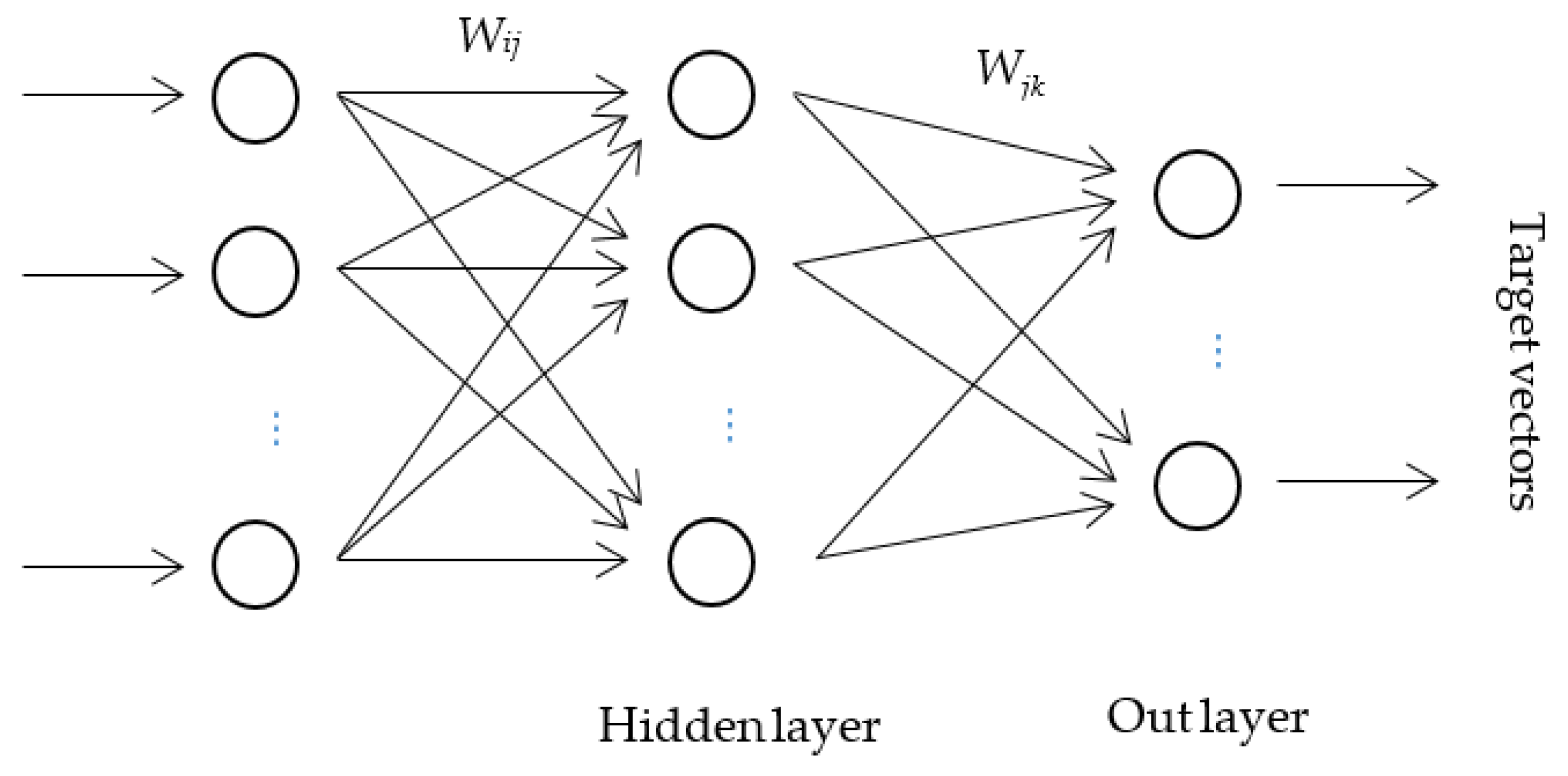
2.3.4. BP Neural Network

The BP neural network is the simplest and most commonly used neural network, and is composed of nonlinear transformed units; it is a multilayer feed-forward neural network and adopts the error back propagation learning algorithm, consisting of an input layer, a hidden layer, and an output layer (Figure 4). Neurons between adjacent layers are connected by weights, whereas neurons in the same layer have no connection, and the transmission function of neurons is a nonlinear function. As a supervised learning network, the logic of the BP neural network is that, for the input learning samples ${\mathrm{P}}_i \left(i=1,2,\dots ,\mathrm{q}\right)$, and their corresponding output samples ${\mathrm{T}}_i \left(i=1,2,\dots ,\mathrm{q}\right)$, the purpose of learning is to correct the weights via the errors between the network output ${\mathrm{A}}_i \left(i=1,2,\dots ,\mathrm{q}\right)$ and the target vectors ${\mathrm{T}}_i \left(i=1,2,\dots ,\mathrm{q}\right)$, rendering the network output as close as possible to the target output and minimizing the sum of the squared errors from the output layer. In order to gradually approximate the target output, it is desirable to continuously calculate the change in the network weight and the deviation in the direction of the decreasing slope relative to the function error, among which the change in the weight and deviation forms the positive correlation with the network error and transmits to each layer with the form of back propagation [65]. In the current study, the BP neural network was implemented using the newff function of the MATLAB software(Ver. R2012a, MathWorks, Inc., Natick, MA, USA).

In the current study, we used 12 satellite images and the 3 monitoring stations in the reservoir; hence, there were a total of 36 groups of in situ ground spectrum measurements. Among the 36 groups of data, the measured TP of monitoring stations 1 and 3 on 30 October 2017 were missing; therefore, these two groups of data were removed, and finally, 34 groups of data were obtained for the training and validation of the BP neural network.

2.3.5. Index Method for Reservoir Eutrophication Evaluation

The trophic state index to determine eutrophication was proposed in 1977 [66]. The current study used five evaluation indexes of Chl-a, CODMn, TN, TP, and SD to classify the trophic condition of Dashahe Reservoir, namely, the “index method”. The formula was as follows:

$$EI=\frac{{{\displaystyle \sum }}_{n=1}^N{E}_n}{N}$$

(3)

where $EI$ is the index of trophic condition (

Table 2. Lakes (reservoirs) eutrophication assessment methods and classification technology requirements.

EI	En	TP (mg/L)	TN (mg/L)	Chl-a (μg/L)	CODMn (mg/L)	SD (m)
Oligotrophic 0 ≤ EI ≤ 20	10	0.001	0.020	0.0005	0.15	10
	20	0.004	0.050	0.0010	0.4	5.0
Mesotrophic 20 < EI ≤ 50	30	0.010	0.10	0.0020	1.0	3.0
	40	0.025	0.30	0.0040	2.0	1.5
	50	0.050	0.50	0.010	4.0	1.0
Meso-eutrophic 50 < EI ≤ 60	60	0.10	1.0	0.026	8.0	0.5
Eutrophic 70 ≤ EI ≤ 80	70	0.20	2.0	0.064	10	0.4
	80	0.60	6.0	0.16	25	0.3
Hype- eutrophic 80 < EI ≤ 100	90	0.90	9.0	0.40	40	0.2
	100	1.3	16.0	1.0	60	0.12

), $E_n$ denotes an assignment score for the $n_{th}$ water quality parameter, and $N$ indicates the number of the water quality parameter used for evaluation. Data in Table 2 are from the technological regulations for surface water resources quality assessment, water conservancy industry standard of the People’s Republic of China (SL395-2007).

3. Results and Discussion

3.1. Model Construction and Verification

Seven wavebands’ (Band1 Coastal, Band2 Blue, Band3 Green, Band4 Red, Band5 NIR, Band6 SWIR1, and Band7 SWIR2) [33,67] reflectance values of remote sensing images and water quality parameters were selected as the input layer and output layer, respectively, and the number of nodes in the hidden layer varied with each inversion model. Therefore, a three-layer BP neural network with the structure of 7 − $i$ − 1, namely, seven nodes (wavebands) in the input layer, $i$ nodes in the hidden layer, and one node (each water quality parameter) in the output layer, was constructed. Because the number of neuron nodes in the hidden layer directly affects the mapping ability of the network, the selection of the number of neuron nodes was the most important step in the design of the BP neural network. However, there is no generally accepted method for the node number selection. If the number of nodes in the hidden layer is too small, the convergence speed of the network is too slow to meet the requirements of accuracy; if the number of nodes is too large, the calculation size will be increased, which also leads to over-fitting and reduces the generalization ability of the network. In the current study, the optimal number of nodes was determined through repeated experiments, namely, an approach of “trial and error”. Twenty-eight groups and the remaining six groups of data were randomly selected for model training and verification, respectively, and finally, the optimal node number ($i$) of each inversion model was identified through multiple trainings (

Table 3. The optimal number nodes in the hidden layer of the BP inversion model.

Model	Chl-a	CODMn	TN	TP	SD
$i$	8	4	10	6	12

). A formal procedure including cross validation in different k-folds, or even the leave one out cross validation (LOOCV), could be further studied for the general design, selection, and validation of the nodes in a BP neural network.

The accuracy of each inversion model was evaluated by the correlation coefficient ($r$), mean relative error ($e$), determination coefficient ($r^2$) [33], and root mean square error ($RMSE$) [68], according to the six groups of inversion value and field observation.

In

Table 4. Evaluation index of accuracy for the BP inversion model.

Model	$\mathit{r}$	$\mathit{e} (\%)$	${\mathit{r}}^2$	$\mathit{R}\mathit{M}\mathit{S}\mathit{E}$
Chl-a	0.94	20.90	0.88	4.81
CODMn	0.81	11.40	0.65	0.42
TN	0.94	17.90	0.87	0.17
TP	0.98	39.80	0.96	0.01
SD	0.93	24.00	0.87	0.41

, $r$ represents the correlation between the inversion value and the field observation, and a larger value of $r$ corresponds to greater correlation. $r^2$ represents the degree of fitting between the inversion value and the field observation, and the closer the $r^2$ to 1, the better the fitting. $RMSE$ indicates the degree of deviation between the inversion value and the field observation, and the closer $RMSE$ to 0, the higher the inversion accuracy. As shown in Table 4, $r^2$ values of the inversion models were above 0.85, except for the inversion model for CODMn. $RMSE$ values of the inversion models for CODMn, TN, TP, and SD were smaller. Although $RMSE$ of the inversion model for Chl-a was larger, the Chl-a inversion model had the minimum relative error (i.e., 6.9%) of the six verified points, and the relative errors of five verified points were less than the average relative error of 20.9%; these points accounted for 82.3%. Overall, the five inversion models performed well and had acceptable accuracy.

In the current study, the inversion model based on the BP neural network was trained and validated according to the field observations of five water quality parameters of three monitoring stations in Dashahe Reservoir and twelve periods of Landsat8 satellite remote sensing images. Overall, the five inversion models performed well and had acceptable accuracy (Table 4). However, the inversion model based on the BP neural network is a data-driven model and its performance largely depends on sample size. In addition, the relative error and RMSE of the five water quality parameters varies when more in situ water measurements and Landsat8 samples are available. However, more data is not always better, and there may be cases of over-fitting [69,70].

3.2. Comparison between the BP Inversion Model and the Multiple Linear Inversion Model

The correlation was calculated between the single band reflectance and thirty-four groups of field observations (

Table 5. The correlation matrix between band reflectance and water quality parameter.

Band/Parameters	lnChl-a	lnCODMn	lnTN	lnTP	lnSD
lnB1	0.35	0.19	−0.11	0.28	−0.02
lnB2	0.17	0.22	0.07	0.30	−0.00
lnB3	−0.17	0.43	0.29	0.38	−0.02
lnB4	−0.11	0.22	0.37	0.46	−0.31
lnB5	0.60	0.11	−0.37	0.34	−0.37
lnB6	0.28	0.08	−0.31	0.50	−0.31
lnB7	0.11	0.02	−0.26	0.46	−0.22

). Then, a multiple linear inversion model was built for each water quality parameter (Equations (4)–(8)) according to 28 groups of field observations. In the multiple linear inversion model, the band reflectance was selected as the independent variable and the water quality parameter was the dependent variable.

Chl-a = 0.001 × B1 + 0.0926 × B2 + 0.009 × B3 − 0.111 × B4 + 0.081 × B5 − 0.075 × B6 + 0.039 × B7 + 6.624 r = 0.65

(4)

CODMn = 0.001 × B1 − 0.002 × B2 + 0.006 × B3 − 0.005 × B4 − 0.002 × B5 + 0.007 × B6 − 0.004 × B7 + 1.465 r = 0.69

(5)

TN = −0.002 × B1 + 0.001 × B2 − 0.001 × B3 + 0.003 × B4 − 0.002 × B5 + 0.009 × B6 − 0.013 × B7 + 1.473 r = −0.80

(6)

TP = −0.00003 × B2 + 0.00003 × B3 + 0.00005 × B4 − 0.00004 × B5 + 0.0005 × B6 − 0.0005 × B7 + 0.002 r = 0.68

(7)

SD = 0.0050 × B2 + 0.0009 × B3 − 0.0058 × B4 + 0.0006 × B5 − 0.0111 × B6 + 0.0125 × B7 + 1.193 r = 0.91

(8)

The remaining six groups of field observations were applied to the multiple linear inversion model and the BP inversion model. The accuracy of the two kinds of inversion model was compared in terms of $e$ and $RMSE$ (

Table 6. Comparison of the evaluation index for the two kinds of inversion model.

Model	$\mathit{e}$ (%)		$\mathit{R}\mathit{M}\mathit{S}\mathit{E}$
	BP Inversion Model	Linear Inversion Model	BP Inversion Model	Linear Inversion Model
Chl-a	20.6	32.6	4.81	10.38
CODMn	11.4	14.0	0.42	0.47
TN	17.9	16.1	0.17	0.14
TP	39.8	48.0	0.01	0.01
SD	24.0	22.7	0.41	0.40

).

As Table 6 shows, the accuracies of the BP inversion models of Chl-a and CODMn were superior to those of the linear inversion models in terms of $e$ and $RMSE$. The accuracies of the two kinds of inversion model for TN, TP, and SD were very close. This is because the fluctuation range of water quality parameters (e.g., TN, TP, and SD) was not obvious, and the samples were concentrated and the number of effective field observation was small. Thus, the inversion value of the multiple linear model approaches a constant value, whereas the BP neural network can adjust the range of learning samples in the input layer to the interval of [−1,1] through normalization. This improves the generalization ability of the model, and ensures the inversion value has the same magnitude and trend as those of the field observations. Taking TP for instance, Isenstein and Park [21] created a multivariate linear regression model ($r^2=0.81 \mathrm{for} \mathrm{TP}$) based on the correlation of the band combinations of imagery and the field observations, and Wu et al. built a regression model ($r^2=0.77$) to characterize the spatial variability of TP, according to the correlation of spectral reflectance with TP concentration. These linear regression models have satisfactory accuracies and help to understand the spatial distribution of TP concentration [71]. However, the linear regression models assume the spectral reflectance has a linear relationship with the TP concentration. In addition, there is a larger fluctuation in the simulated TP concentration when using the linear regression equations, which may be not consistent with the in situ ground spectrum measurement. In general, the BP inversion model performs better for the inversion of the water quality parameters of Dashahe Reservoir than the linear inversion model.

3.3. Change in Water Quality Parameters and Reservoir Eutrophication Evaluation

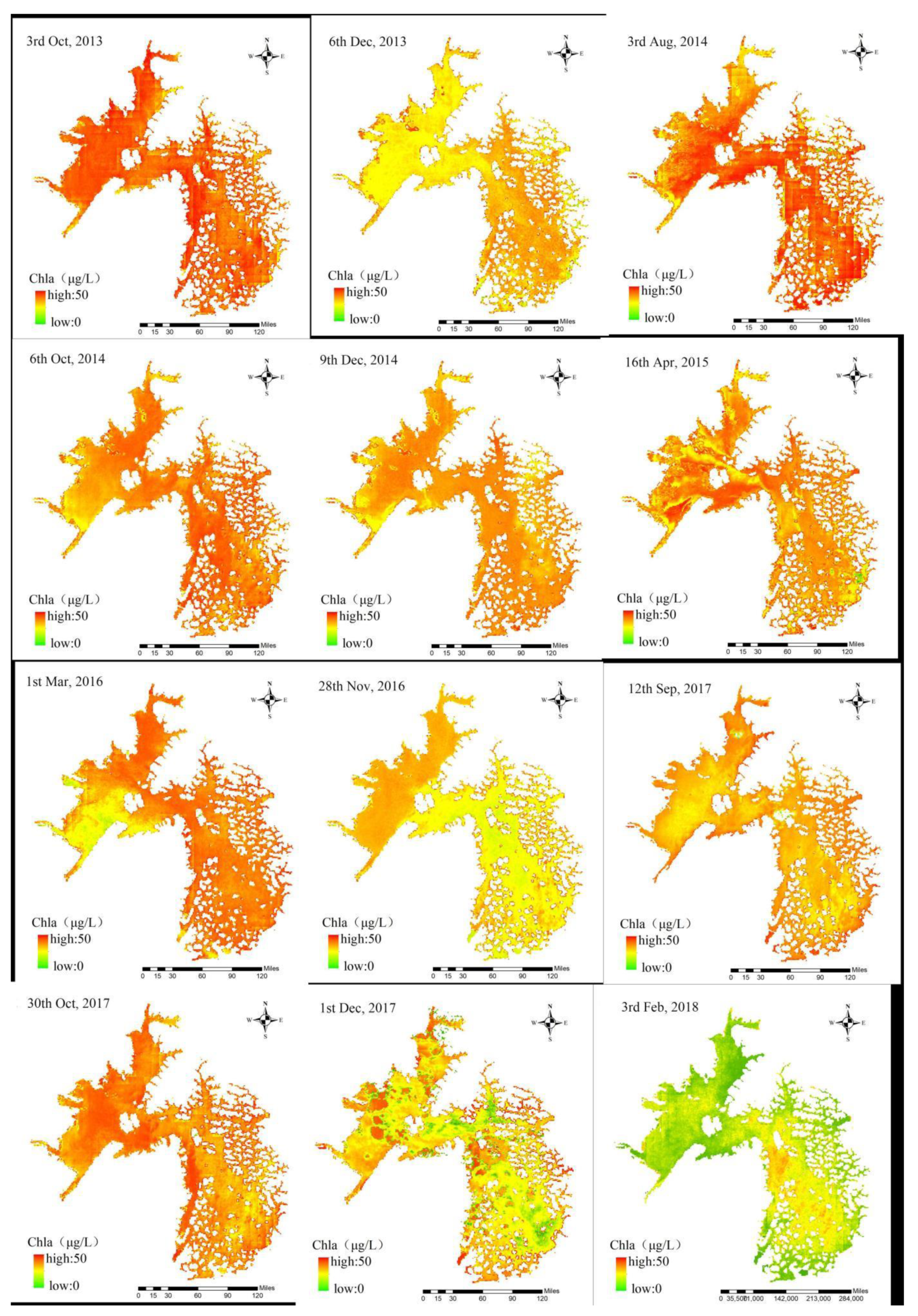
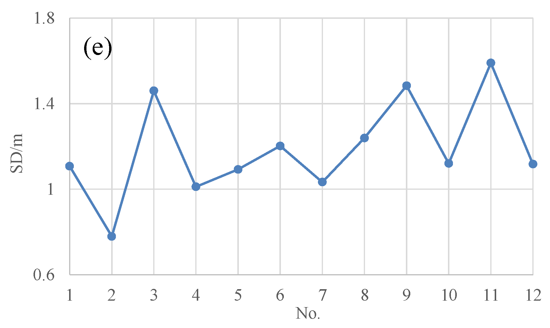
3.3.1. Change in Water Quality Parameters in Dashahe Reservoir

The concentrations of water quality parameters in each pixel were obtained by the BP inversion models according to the multi-temporal remote sensing images of Dashahe Reservoir, and continuous water quality parameter monitoring was conducted across the whole reservoir. The concentration of water quality parameters obtained by the inversion model in different pixels were output in different colors to show the spatial distributions of the concentrations of the water quality parameters of Dashahe reservoir. Taking Chl-a for instance (Figure 5), the concentrations of Chl-a in the five periods (i.e., 3 October 2013, 3 August 2014, 6 October 2014, 1 March 2016, and 30 October 2017) were higher than those in other periods and showed an obvious seasonal variation. The temperature of Dashahe Reservoir in spring and autumn encourages aquatic algae to multiply rapidly with high density, resulting in an increase in the concentration of Chl-a, whereas the concentration of Chl-a decreases in winter, mainly due to low temperature and low density of algae. In general, the concentration of Chl-a was evenly distributed in the three periods (i.e., 3 October 2013, 3 August 2014, and 12 September 2017) across the reservoir and showed a spatial difference in other periods. For example, in the period of 3 February 2018, the concentration of Chl-a was higher in the central and southern part of Dashahe Reservoir, and lower in the northwest region, and the maximum and mean values were 46.02 and 18.32 μg/L, respectively. Figure 6a also illustrates that the concentration of Chl-a was higher in spring and autumn, and the average concentration of CODMn exceeded the surface water Class Ⅱ water standard on 16 April 2015 and 1 December 2017 (Figure 6b); the concentration of TN exceeded the surface water Class Ⅱ water standard during the twelve periods (Figure 6c); and the concentration of TP also exceeded the surface water Class Ⅱ water standard on 6 October 2014, 16 April 2015, and 1 March 2016 (Figure 6d). In addition, the mean SD was the worst on 6 December 2013, with visibility of 0.799 m, due to significant suspended solids in water, and the best SD occurred on 1 December 2017, with visibility of 1.59 m (Figure 6e).

3.3.2. Evaluation of Trophic Condition at Dashahe Reservoir

As shown in

Table 7. Area proportion of trophic condition in different periods at Dashahe Reservoir.

Date	Proportion
	Mesotrophy	Meso-Eutrophy	Eutrophy
3 October 2013	79.84%	20.11%	0.05%
6 December 2013	53.01%	46.95%	0.04%
3 August 2014	74.10%	25.86%	0.05%
6 October 2014	45.68%	52.94%	1.38%
9 December 2014	39.69%	60.15%	0.15%
16 April 2015	48.39%	50.68%	0.93%
1 March 2016	28.78%	71.18%	0.04%
28 November 2016	93.70%	6.25%	0.06%
12 September 2017	90.89%	9.11%	0.00%
30 October 2017	63.86%	35.83%	0.31%
1 December 2017	89.30%	10.69%	0.01%
3 February 2018	95.66%	4.33%	0.00%

, overall, Dashahe Reservoir was in the state of mesotrophication and light eutrophication, among which light eutrophication accounted for the largest proportions in March, April, October, and December, and mid-eutrophication had the largest proportion on 6 October 2014.

The area of light eutrophication accounted for larger proportions in March, April, October, and December. In addition, the concentration of Chl-a was higher in spring and autumn, and TP at Dashahe Reservoir exceeded the surface water Class Ⅱ water standard on 6 October 2014, 9 December 2015, and 1 March 2016. Large amounts of untreated domestic sewage within the watershed are discharged via open ditches into the tributaries, and livestock production mainly occurs around the reservoir in small fenced areas with high stocking densities. Ducks and geese are occasionally housed in enclosures, but also inhabit streams and rivers. Chicken farms typically discharge directly into streams and pig production is also typically close to fish ponds where excreta are discharged directly into waterways. In addition, the water quality of the watershed is also affected by the excessive use of fertilizers and pesticides for agricultural production in the surrounding areas. Point and non-point sources of pollution within the watershed have resulted in nutrient loading in Dashahe Reservoir [53]. Appropriate temperatures in spring and autumn contribute to algae blooms [72], in addition to the polluted inflow of the reservoir. These may contribute to the light eutrophication status of Dashahe Reservoir. From April to September, Dashahe Reservoir was in a state of mesotrophication. This is because the water body of the reservoir is rapidly updated by the frequent rainfall that occurs in the rainy season.

The reservoir was divided into three evaluation areas (Figure 7), namely, the inflowing area, the middle area, and the outflowing area, and $EI$ for each area was calculated. Taking the remote sensing image of 6 October 2014 as an example, $EI$ values for the inflowing, middle, and outflowing areas were 53.9, 50.2, and 49.5, respectively, thus showing a decreasing $EI$ from the inflowing area to the outflowing area of the reservoir. The inflowing area was in the state of light eutrophication and had the largest $EI$, indicating that the inflow of Dashahe Reservoir was the main source of nutrient salts. The inflowing areas of the reservoir are surrounded by fish ponds and scattered fenced areas, and livestock production and domestic sewage around this area result in a large nutrient loading in the inflow, which exacerbates the eutrophication condition of the reservoir. Therefore, it is necessary to implement buffer zones around the reservoir and remove sewage discharges to achieve a marked improvement in the reservoir water quality.

4. Conclusions

In the current study, a remote sensing inversion model based on a BP neural network was constructed to simulate the water quality parameters of inland Case-2 water bodies, such as reservoirs, and provide a basis for reservoir eutrophication evaluation. The BP inversion model was applied to simulate five water quality parameters (Chl-a, CODMn, SD, TP, and TN) of Dashahe Reservoir, a typical inland Case-2 water body in South China, using twelve periods of remote sensing images and field observations. The accuracy of the BP inversion model was compared with that of the multiple linear inversion model. This study provides technical support for the monitoring of reservoir water quality parameters and reservoir eutrophication evaluation at an extensive scale and in continuous space. The main findings were as follows:

(1)

The preprocessing of remote sensing images helps to highlight spectral information by eliminating the influence of reflectance on objects caused by atmospheric aerosols and removing noise. This effectively restores the real reflectance after radiation calibration and atmospheric correction.

(2)

The BP inversion model was built for each of the five water quality parameters of Dashahe Reservoir and the optimal node number of each inversion model was identified through multiple trainings. The accuracy of the BP inversion models of Chl-a and CODMn was superior to that of the multiple linear inversion models, due to the improved generalization of the BP neural network. The performance of the BP inversion model was better than that of the multiple linear inversion model when the water quality parameters had a larger fluctuation range.

(3)

Overall, Dashahe Reservoir was in the state of mesotrophication and light eutrophication. The area of light eutrophication accounted for larger proportions in spring and autumn due to algae blooms driven by appropriate temperatures and polluted reservoir inflows around the reservoir. The reservoir inflow was the main source of nutrient salts in Dashahe Reservoir.

It can be concluded that, combined with field observations, remote sensing technology has the potential to comprehensively and dynamically reflect the distribution of the concentration of reservoir water quality parameters and overcome the disadvantages of conventional water quality monitoring methods. The local water resource department can identify the trend in the water quality of Dashahe Reservoir using the long-term and dynamic remote sensing monitoring based on the multi-temporal remote sensing images with high spatial and temporal resolution, and implement water pollution prevention and control strategies according to the real-time change in reservoir water quality.

The BP inversion model performs better in simulating the water quality parameters of inland Case-2 water bodies, such as Dashahe Reservoir, if there are rich field observations. In the current study, the eutrophication evaluation results are only applicable to the Dashahe Reservoir. However, the inversion model based on the BP neural network may be applied to other reservoirs when samples between in situ water measurements and satellite remote sensing images are available. The current study examined the data of three monitoring stations, and some field observations of water quality parameters (e.g., TP, TN, and SD) were not available. Therefore, the accuracy of the BP inversion model can be further improved if new monitoring stations and field observations are available.

References

1. Shourian, M.; Moridi, A.; Kaveh, M. Modeling of eutrophication and strategies for improvement of water quality in reservoirs. Water Sci. Technol. 2016, 74, 1376–1385. [Google Scholar] [CrossRef]
2. Li, Z.; Ma, J.R.; Guo, J.S.; Paerl, H.W.; Brookes, J.D.; Xiao, Y.; Fang, F.; Ouyang, W.J.; Lu, L.H. Water quality trends in the Three Gorges Reservoir region before and after impoundment (1992–2016). Ecohydrol. Hydrobiol. 2019, 19, 317–327. [Google Scholar] [CrossRef]
3. Yang, W.; Yao, J.M.; He, Y.Z.; Huang, Y.Y.; Liu, H.Z.; Zhi, Y.; Qian, S.H.; Yan, X.M.; Jian, S.; Li, W. Nitrogen removal enhanced by benthic bioturbation coupled with biofilm formation: A new strategy to alleviate freshwater eutrophication. J. Environ. Manag. 2021, 292, 112814. [Google Scholar] [CrossRef]
4. Smith, V.H.; Tilman, G.D.; Nekola, J.C. Eutrophication: Impacts of excess nutrient inputs on freshwater, marine, and terrestrial ecosystems. Environ. Pollut. 1999, 100, 179–196. [Google Scholar] [CrossRef]
5. Vieira, J.M.P.; Pinho, J.L.S.; Dias, N.; Schwanenberg, D.; Van den Boogaard, H.F.P. Parameter estimation for eutrophication models in reservoirs. Water Sci. Technol. 2013, 68, 319–327. [Google Scholar] [CrossRef] [PubMed]
6. Smith, V.H.; Schindler, D.W. Eutrophication science: Where do we go from here? Trends Ecol. Evol. 2009, 24, 201–207. [Google Scholar] [CrossRef] [PubMed]
7. Sayers, M.J.; Bosse, K.R.; Shuchman, R.A.; Ruberg, S.A.; Fahnenstiel, G.L.; Leshkevich, G.A.; Stuart, D.G.; Johengen, T.H.; Burtner, A.M.; Palladino, D. Spatial and temporal variability of inherent and apparent optical properties in western Lake Erie: Implications for water quality remote sensing. J. Great Lakes Res. 2019, 45, 490–507. [Google Scholar] [CrossRef]
8. Schaeffer, B.; Schaeffer, K.G.; Keith, D.; Lunetta, R.S.; Conmy, R.; Gould, R.W. Barriers to adopting satellite remote sensing for water quality management. Int. J. Remote Sens. 2013, 34, 7534–7544. [Google Scholar] [CrossRef]
9. Kim, H.C.; Son, S.; Kim, Y.H.; Khim, J.S.; Nam, J.; Chang, W.K.; Lee, J.H.; Lee, C.H.; Ryu, J. Remote sensing and water quality indicators in the Korean West coast: Spatio-temporal structures of MODIS-derived chlorophyll-a and total suspended solids. Mar. Pollut. Bull. 2017, 121, 425–434. [Google Scholar] [CrossRef]
10. Anding, D.; Kauth, R. Estimation of sea surface temperature from space. Remote Sens. Environ. 1970, 1, 217–220. [Google Scholar] [CrossRef] [Green Version]
11. Morel, A.; Prieur, L. Analysis of variations in ocean color1. Limnol. Oceanogr. 1977, 22, 709–722. [Google Scholar] [CrossRef]
12. Dlamini, S.; Nhapi, I.; Gumindoga, W.; Nhiwatiwa, T.; Dube, T. Assessing the feasibility of integrating remote sensing and in-situ measurements in monitoring water quality status of Lake Chivero, Zimbabwe. Phys. Chem. Earth Parts A/B/C 2016, 93, 2–11. [Google Scholar] [CrossRef]
13. Alikas, K.; Kratzer, S. Improved retrieval of Secchi depth for optically-complex waters using remote sensing data. Ecol. Indic. 2017, 77, 218–227. [Google Scholar] [CrossRef]
14. Seyhan, E.; Dekker, A. Application of remote sensing techniques for water quality monitoring. Hydrobiol. Bull. 1986, 20, 41–50. [Google Scholar] [CrossRef]
15. Kondratyev, K.Y.; Pozdnyakov, D.V.; Pettersson, L.H. Water quality remote sensing in the visible spectrum. Int. J. Remote Sens. 1998, 19, 957–979. [Google Scholar] [CrossRef]
16. Wang, X.J.; Ma, T. Application of remote sensing techniques in monitoring and assessing the water quality of Taihu Lake. Bull. Environ. Contam. Toxicol. 2001, 67, 863–870. [Google Scholar] [CrossRef]
17. Koponen, S.; Pulliainen, J.; Kallio, K.; Hallikainen, M. Lake water quality classification with airborne hyperspectral spectrometer and simulated MERIS data. Remote Sens. Environ. 2002, 79, 51–59. [Google Scholar] [CrossRef]
18. Gower, J.; King, S.; Borstad, G.; Brown, L. Detection of intense plankton blooms using the 709 nm band of the MERIS imaging spectrometer. Int. J. Remote Sens. 2005, 26, 2005–2012. [Google Scholar] [CrossRef]
19. Matthews, M.W. A current review of empirical procedures of remote sensing in inland and near-coastal transitional waters. Int. J. Remote Sens. 2011, 32, 6855–6899. [Google Scholar] [CrossRef]
20. Imen, S.; Chang, N.-B.; Yang, Y.J. Developing the remote sensing-based early warning system for monitoring TSS concentrations in Lake Mead. J. Environ. Manag. 2015, 160, 73–89. [Google Scholar] [CrossRef]
21. Isenstein, E.M.; Park, M.H. Assessment of nutrient distributions in Lake Champlain using satellite remote sensing. J. Environ. Sci. 2014, 26, 1831–1836. [Google Scholar] [CrossRef]
22. Politi, E.; Cutler, M.E.J.; Rowan, J.S. Evaluating the spatial transferability and temporal repeatability of remote-sensing-based lake water quality retrieval algorithms at the European scale: A meta-analysis approach. Int. J. Remote Sens. 2015, 36, 2995–3023. [Google Scholar] [CrossRef] [Green Version]
23. Wu, J.; Li, Z.B.; Zhu, L.; Li, G.Y.; Niu, B.S.; Peng, F. Optimized BP neural network for dissolved oxygen prediction. IFAC-PapersOnLine 2018, 51, 596–601. [Google Scholar] [CrossRef]
24. Heege, T.; Kiselev, V.; Wettle, M.; Hung, N.N. Operational multi-sensor monitoring of turbidity for the entire Mekong delta. Int. J. Remote Sens. 2014, 35, 2910–2926. [Google Scholar] [CrossRef]
25. Lymburner, L.; Botha, E.; Hestir, E.; Anstee, J.; Sagar, S.; Dekker, A.; Malthus, T. Landsat 8: Providing continuity and increased precision for measuring multi-decadal time series of total suspended matter. Remote Sens. Environ. 2016, 185, 108–118. [Google Scholar] [CrossRef]
26. Malthus, T.J.; Hestir, E.L.; Dekker, A.G.; Brando, V.E. The case for a global inland water quality product. In Proceedings of the 2012 IEEE International Geoscience and Remote Sensing Symposium, Munich, Germany, 22–27 July 2012; pp. 5234–5237. [Google Scholar]
27. Gholizadeh, M.H.; Melesse, A.M.; Reddi, L. A comprehensive review on water quality parameters estimation using remote sensing techniques. Sensors 2016, 16, 1298. [Google Scholar] [CrossRef] [Green Version]
28. Tanaka, A.; Kishino, M.; Oishi, T.; Doerffer, R.; Schiller, H. Application of neural network method to case II water. In Proceedings of the Remote Sensing of the Ocean and Sea Ice, Barcelona, Spain, 28–29 September 2000; Volume 4172, pp. 144–153. [Google Scholar] [CrossRef]
29. Moore, G.F.; Aiken, J.; Lavender, S.J. The atmospheric correction of water colour and the quantitative retrieval of suspended particulate matter in Case II waters: Application to MERIS. Int. J. Remote Sens. 1999, 20, 1713–1733. [Google Scholar] [CrossRef]
30. Qin, B. Lake eutrophication: Control countermeasures and recycling exploitation. Ecol. Eng. 2009, 35, 1569–1573. [Google Scholar] [CrossRef]
31. Mamun, M.; Kim, J.J.; Alam, M.A.; An, K.G. Prediction of algal chlorophyll-a and water clarity in monsoon-region reservoir using machine learning approaches. Water 2019, 12, 30. [Google Scholar] [CrossRef] [Green Version]
32. Jiang, Y.P.; Xu, Z.X.; Yin, H.L. Study on improved BP artificial neural networks in eutrophication assessment of China eastern lakes. J. Hydrodyn. 2006, 18, 528–532. [Google Scholar] [CrossRef]
33. Lu, F.; Chen, Z.; Liu, W.Q.; Shao, H.B. Modeling chlorophyll-a concentrations using an artificial neural network for precisely eco-restoring lake basin. Ecol. Eng. 2016, 95, 422–429. [Google Scholar] [CrossRef]
34. Kuo, J.T.; Hsieh, M.H.; Lung, W.S.; She, N. Using artificial neural network for reservoir eutrophication prediction. Ecol. Model. 2007, 200, 171–177. [Google Scholar] [CrossRef]
35. Chang, N.B.; Xuan, Z.M.; Yang, Y.J. Exploring spatiotemporal patterns of phosphorus concentrations in a coastal bay with MODIS images and machine learning models. Remote Sens. Environ. 2013, 134, 100–110. [Google Scholar] [CrossRef]
36. Zheng, Z.B.; Li, Y.M.; Guo, Y.L.; Xu, Y.F.; Liu, G.; Du, C.G. Landsat-based long-term monitoring of total suspended matter concentration pattern change in the wet season for Dongting Lake, China. Remote Sens. 2015, 7, 13975–13999. [Google Scholar] [CrossRef] [Green Version]
37. Song, K.S.; Wang, Z.M.; Blackwell, J.; Zhang, B.; Li, F.; Zhang, Y.Z.; Jiang, G.J. Water quality monitoring using Landsat Themate Mapper data with empirical algorithms in Chagan Lake, China. J. Appl. Remote Sens. 2011, 5, 53506. [Google Scholar] [CrossRef]
38. Chang, N.-B.; Vannah, B.W.; Yang, Y.J.; Elovitz, M. Integrated data fusion and mining techniques for monitoring total organic carbon concentrations in a lake. Int. J. Remote Sens. 2014, 35, 1064–1093. [Google Scholar] [CrossRef]
39. Sun, D.; Qiu, Z.; Li, Y.; Shi, K.; Gong, S. Detection of total phosphorus concentrations of turbid inland waters using a remote sensing method. Water Air Soil Pollut. 2014, 225, 1953. [Google Scholar] [CrossRef]
40. Lin, S.; Novitski, L.N.; Qi, J.; Stevenson, R.J. Landsat TM/ETM+ and machine-learning algorithms for limnological studies and algal bloom management of inland lakes. J. Appl. Remote Sens. 2018, 12, 026003. [Google Scholar] [CrossRef]
41. Topp, S.N.; Pavelsky, T.M.; Jensen, D.; Simard, M.; Ross, M.R.V. Research trends in the use of remote sensing for inland water quality science: Moving towards multidisciplinary applications. Water 2020, 12, 169. [Google Scholar] [CrossRef] [Green Version]
42. Arias-Rodriguez, L.F.; Duan, Z.; Sepúlveda, R.; Martinez-Martinez, S.I.; Disse, M. Monitoring water quality of valle de bravo reservoir, Mexico, using entire lifespan of MERIS data and machine learning approaches. Remote Sens. 2020, 12, 1586. [Google Scholar] [CrossRef]
43. Holyoak, K.J. A Connectionist view of cognition: Parallel distributed processing. Science 1987, 236, 992–996. [Google Scholar] [CrossRef]
44. Keiner, L.E.; Yan, X.-H. A Neural network model for estimating sea surface chlorophyll and sediments from thematic mapper imagery. Remote Sens. Environ. 1998, 66, 153–165. [Google Scholar] [CrossRef]
45. Schiller, H.; Doerffer, R. Neural network for emulation of an inverse model operational derivation of Case II water properties from MERIS data. Int. J. Remote Sens. 1999, 20, 1735–1746. [Google Scholar] [CrossRef]
46. Liu, J.; Zhang, Y.; Yuan, D.; Song, X. Empirical estimation of total nitrogen and total phosphorus concentration of urban water bodies in China using high resolution IKONOS multispectral imagery. Water 2015, 7, 6551–6573. [Google Scholar] [CrossRef] [Green Version]
47. Ioannou, I.; Gilerson, A.; Gross, B.; Moshary, F.; Ahmed, S. Deriving ocean color products using neural networks. Remote Sens. Environ. 2013, 134, 78–91. [Google Scholar] [CrossRef]
48. Du, C.; Wang, Q.; Li, Y.; Lyu, H.; Zhu, L.; Zheng, Z.; Wen, S.; Liu, G.; Guo, Y. Estimation of total phosphorus concentration using a water classification method in inland water. Int. J. Appl. Earth Obs. Geoinf. 2018, 71, 29–42. [Google Scholar] [CrossRef]
49. Bai, Y.; Gao, J.; Zhang, Y. Research on wind-induced nutrient release in Yangshapao Reservoir, China. Water Supply 2020, 20, 469–477. [Google Scholar] [CrossRef]
50. Khan, M.S.; Suhail, M.; Alharbi, T. Evaluation of urban growth and land use transformation in Riyadh using Landsat satellite data. Arab. J. Geosci. 2018, 11, 1–13. [Google Scholar] [CrossRef]
51. Wang, D.; Ma, R.; Xue, K.; Loiselle, S.A. The assessment of landsat-8 OLI atmospheric correction algorithms for inland waters. Remote Sens. 2019, 11, 169. [Google Scholar] [CrossRef] [Green Version]
52. Sahana, M.; Dutta, S.; Sajjad, H. Assessing land transformation and its relation with land surface temperature in Mumbai city, India using geospatial techniques. Int. J. Urban Sci. 2019, 23, 205–225. [Google Scholar] [CrossRef]
53. Nielsen, A.; Trolle, D.; Me, W.; Luo, L.; Han, B.-P.; Liu, Z.; Olesen, J.E.; Jeppesen, E. Assessing ways to combat eutrophication in a Chinese drinking water reservoir using SWAT. Mar. Freshw. Res. 2013, 64, 475–492. [Google Scholar] [CrossRef] [Green Version]
54. Woo, M.-K.; Huang, L.; Zhang, S.; Li, Y. Rainfall in Guangdong province, South China. Catena 1997, 29, 115–129. [Google Scholar] [CrossRef]
55. Tiwari, A.; Oliver, D.; Bivins, A.; Sherchan, S.; Pitkänen, T. Bathing water quality monitoring practices in Europe and the United States. Int. J. Environ. Res. Public Health 2021, 18, 5513. [Google Scholar] [CrossRef] [PubMed]
56. Wang, K.; Jiang, Q.-G.; Yu, D.-H.; Yang, Q.-L.; Wang, L.; Han, T.-C.; Xu, X.-Y. Detecting daytime and nighttime land surface temperature anomalies using thermal infrared remote sensing in Dandong geothermal prospect. Int. J. Appl. Earth Obs. Geoinf. 2019, 80, 196–205. [Google Scholar] [CrossRef]
57. Rani, N.; Mandla, V.R.; Singh, T. Evaluation of atmospheric corrections on hyperspectral data with special reference to mineral mapping. Geosci. Front. 2017, 8, 797–808. [Google Scholar] [CrossRef] [Green Version]
58. Zeng, Q.; Zhao, Y.; Tian, L.Q.; Chen, X.L. Evaluation on the atmospheric correction methods for water color remote sensing by using HJ-1A/1B CCD image-taking Poyang Lake in China as a case. Spectrosc. Spectr. Anal. 2013, 33, 1320–1326. [Google Scholar]
59. Bernardo, N.; Watanabe, F.; Rodrigues, T.; Alcântara, E. Atmospheric correction issues for retrieving total suspended matter concentrations in inland waters using OLI/Landsat-8 image. Adv. Space Res. 2017, 59, 2335–2348. [Google Scholar] [CrossRef] [Green Version]
60. Cao, Y.; Ye, Y.; Zhao, H.; Jiang, Y.; Wang, H.; Shang, Y.; Wang, J. Remote sensing of water quality based on HJ-1A HSI imagery with modified discrete binary particle swarm optimization-partial least squares (MDBPSO-PLS) in inland waters: A case in Weishan Lake. Ecol. Inform. 2018, 44, 21–32. [Google Scholar] [CrossRef]
61. Moses, W.; Gitelson, A.A.; Perk, R.L.; Gurlin, D.; Rundquist, D.C.; Leavitt, B.C.; Barrow, T.M.; Brakhage, P. Estimation of chlorophyll-a concentration in turbid productive waters using airborne hyperspectral data. Water Res. 2012, 46, 993–1004. [Google Scholar] [CrossRef] [Green Version]
62. Eugenio, F.; Marcello, J.; Martin, J.; Rodríguez-Esparragón, D. Benthic habitat mapping using multispectral high-resolution imagery: Evaluation of shallow water atmospheric correction techniques. Sensors 2017, 17, 2639. [Google Scholar] [CrossRef] [Green Version]
63. Lu, S.; Wu, B.; Yan, N.; Wang, H. Water body mapping method with HJ-1A/B satellite imagery. Int. J. Appl. Earth Obs. Geoinf. 2011, 13, 428–434. [Google Scholar] [CrossRef]
64. McFeeters, S.K. The use of the normalized difference water index (NDWI) in the delineation of open water features. Int. J. Remote Sens. 1996, 17, 1425–1432. [Google Scholar] [CrossRef]
65. He, Y.; Chen, S.; Huang, R.; Chen, X.; Cong, P. Impact of upstream runoff and tidal level on the chlorinity of an estuary in a river network: A case study of Modaomen estuary in the Pearl River Delta, China. J. Hydroinform. 2019, 21, 359–370. [Google Scholar] [CrossRef]
66. Carlson, R.E. A trophic state index for lakes1 Limnology and oceanography. Limnol. Oceanogr. 1977, 22, 361–369. [Google Scholar] [CrossRef] [Green Version]
67. Nazeer, M.; Nichol, J.E. Development and application of a remote sensing-based Chlorophyll-a concentration prediction model for complex coastal waters of Hong Kong. J. Hydrol. 2016, 532, 80–89. [Google Scholar] [CrossRef]
68. Wu, Z.; Wang, X.; Chen, Y.; Cai, Y.; Deng, J. Assessing river water quality using water quality index in Lake Taihu Basin, China. Sci. Total Environ. 2018, 612, 914–922. [Google Scholar] [CrossRef] [PubMed]
69. Deng, Q. A BP neural network optimisation method based on dynamical regularization. J. Control. Decis. 2017, 6, 111–121. [Google Scholar] [CrossRef]
70. Zhang, H.Q. BP neural network and its improved algorithm in the power system transformer fault diagnosis. Appl. Mech. Mater. 2013, 418, 200–204. [Google Scholar] [CrossRef]
71. Wu, C.; Wu, J.; Qi, J.; Zhang, L.; Huang, H.; Lou, L.; Chen, Y. Empirical estimation of total phosphorus concentration in the mainstream of the Qiantang River in China using Landsat TM data. Int. J. Remote Sens. 2010, 31, 2309–2324. [Google Scholar] [CrossRef]
72. Hao, C.; Wei, P.; Pei, L.; Du, Z.; Zhang, Y.; Lu, Y.; Dong, H. Significant seasonal variations of microbial community in an acid mine drainage lake in Anhui Province, China. Environ. Pollut. 2017, 223, 507–516. [Google Scholar] [CrossRef]
Figure 1. Location of the Dashahe Reservoir.
Water 13 02844 g001
Figure 2. Spectral curves of waters and vegetation: (a) before atmospheric correction and (b) after atmospheric correction.
Water 13 02844 g002
Figure 3. Water extraction by the NDWI method: (a) water mask and (b) after water extraction.
Water 13 02844 g003
Figure 4. Three layers of the BP neural network.
Water 13 02844 g004
Figure 5. Distribution of the concentration of Chl-a across the Dashahe Reservoir.
Water 13 02844 g005
Figure 6. The trend of the concentration of water quality parameters in Dashahe Reservoir: (a) Chl-a, (b) CODMn, (c) TN, (d) TP, and (e) SD.
Water 13 02844 g006aWater 13 02844 g006b
Figure 7. Evaluation area of the trophic condition in the Dashahe Reservoir.
Water 13 02844 g007