
Smoothed Particle Hydrodynamics Simulation of a Mariculture Platform under Waves


1
College of Ocean & Earth Sciences, Xiamen University, Xiamen 361005, China
2
Fujian Provincial Academy of Environmental Science, Fuzhou 350003, China
3
Fujian Engineering and Research Center of Safety Control for Ship Intelligent Navigation, Minjiang University, Fuzhou 350108, China
*
Authors to whom correspondence should be addressed.
Water 2021, 13(20), 2847; https://doi.org/10.3390/w13202847
Submission received: 16 August 2021
/
Revised: 29 September 2021
/
Accepted: 9 October 2021
/
Published: 13 October 2021
(This article belongs to the Section Biodiversity and Functionality of Aquatic Ecosystems)
Abstract
:This work investigates the dynamic behaviors of floating structures with moorings using open-source software for smoothed particle hydrodynamics. DualSPHysics permits us to use graphics processing units to recreate designs that include complex calculations at high resolution with reasonable computational time. A free damped oscillation was simulated, and its results were compared with theoretical data to validate the numerical model developed. The simulated three degrees of freedom (3-DoF) (surge, heave, and pitch) of a rectangular floating box have excellent consistency with experimental data. MoorDyn was coupled with DualSPHysics to include a mooring simulation. Finally, we modelled and simulated a real mariculture platform on the coast of China. We simulated the 3-DoF of this mariculture platform under a typical annual wave and a Typhoon Dujuan wave. The motion was light and gentle under the typical annual wave but vigorous under the Typhoon Dujuan wave. Experiments at different tidal water levels revealed an earlier motion response and smaller motion range during the high tide. The results reveal that DualSPHysics combined with MoorDyn is an adaptive scheme to simulate a coupled fluid–solid–mooring system. This work provides support to disaster warning, emergency evacuation, and proper engineering design.
1. Introduction
In the ocean, the interactions between water and boats, bridge piers, wharves, and offshore engineering platforms are of great concern. The dynamic behavior of floating structures is considered a fluid–solid interaction. Gabl [1] presents the experimental results of a simplified geometry floating in a wave tank under regular wave conditions, and expands the previous experimental investigation and focuses on the mooring system to identify the potential influences on modelling assumptions [2] Numerically simulating fluid–solid interaction is difficult owing to the complex geometries and violent hydrodynamics involved. In recent work, Palm et al. [3] coupled a CFD model, the OpenFOAM solver, and the Moody high-order finite element model of mooring cables to study fluid–solid interaction. Fernandes et al. [4] studied the fluid–solid interaction between particles and Newtonian fluids. Galuppo et al. [5] studied the fluid–solid interaction of complex viscoelastic fluids. Gu H, Peter S., Tim S., et al. used the advanced CFD software STAR-CCM+ to simulate forced heave and surge motion of axisymmetric vertical cylindrical bodies with flat and rounded [6].
Smoothed particle hydrodynamics (SPH) is a meshless method with a simple mathematical formulation and high computational efficiency that overcomes the limitations of mesh-based methods. Domínguez et al. [7] first coupled SPH with a dynamic mooring model and achieved good validation of the structural motions and mooring forces.
DualSPHysics is a numerical modelling code based on SPH. DualSPHysics is efficient and user-friendly, and has been widely used in hydraulic, naval, and coastal engineering. Engineering problems with high resolution can be simulated by DualSPHysics in a reasonable time owing to the power of graphics processing units (GPUs), which are graphics cards with powerful parallel computing. The advantages of using GPUs to simulate the Navier–Stokes equations can be found in [8]. DualSPHysics has been demonstrated to accurately predict flows in coastal engineering [9,10,11,12]. It has reproduced wave propagation, wave transformation, and interaction between waves and structures. The code of DualSPHysics is used to mimic experimental facilities like a wave flume and wave basin. DualSPHysics includes automatic wave generation and wave absorption. The moving boundaries in DualSPHysics are used to mimic a piston-type wavemaker to generate regular waves with the desired height and period. Passive and active wave absorption can both be configured in DualSPHysics. In passive absorption, sponge layers or a dissipative beach are used to absorb the waves reflected there, while active wave absorption is used to avoid the effect of backward-travelling waves on the numerical piston. The author of [13] describes passive and active absorption techniques and wave generation algorithms in detail.
MoorDyn [14], the multi-segmented and lumped-mass mooring dynamics model, represents the behavior of a mooring line. MoorDyn computes common offshore mooring scenarios efficiently and accurately [15,16]. Lee et al. coupled the open-source libraries MoorDyn and OpenFOAM bi-directionally [17]. Quartier et al. [18] coupled DualSPHysics and Project Chrono to investigate power take-off (PTO) systems of a wave energy converter (WEC). Pribadi et al. [19] used the lumped-mass open-source code MoorDyn to simulate the behavior of a mussel longline system subjected to waves and current loads.
MoorDyn is open source, and it is coupled with DualSPHysics here to model fluid–solid interaction with moorings to enable a more accurate analysis for a moored platform.
This paper is organized into five sections. Section 1 is the introduction. Section 2 describes the SPH model. Section 3 shows the validations for the decay structure and the freely floating and moored floating structures under regular waves. Section 4 applies the SPH model to one of China’s coastal mariculture platforms. Section 5 presents the main conclusions of this work.
The aim of this paper is to model the hydrodynamic fluid–solid interaction under waves and to compute mariculture platform movements under actual incident wave conditions on the Chinese coast.
2. SPH Model
DualSPHysics [20] is an open-source program developed at Universidade de Vigo (Spain) and University of Manchester (UK). DualSPHysics uses SPH for actual engineering issues. It can be run on either CPUs or GPU cards. GPUs currently offer higher processing power than CPUs and are a reasonable alternative for accelerating SPH at low financial cost. Consequently, DualSPHysics can run on a PC into which a GPU card is introduced. In addition, there are some cases where high resolution in time and space is needed when relevant modes of interaction are not generally clear. This requires advanced codes and executions for some large-domain simulations, which makes DualSPHysics ideal because it is the most proficient SPH code overall [21].
The DualSPHysics code can be downloaded freely from www.dual.sphysics.org (accessed on 10 August 2021). Details and information about it can be found in [20,22]. DualSPHysics has been applied to beach front design issues, such as assessing the collection of real waterfront obstructions [23] and evaluating the effect of waves on seaside structures [24].
2.1. SPH Method
The meshless Lagrangian SPH method uses a set of material points or particles to discretize a continuum. These particles are associated with their own individual properties (mass, density, velocity, and pressure). The governing equations are integrated at the particle locations using an interpolation function called a kernel function (W).
A function can be defined in as:
where is the kernel function, is the smoothed length, and represents the position vector of the particle.
A discrete approximation of the vector function in Equation (1) at particle is:
where is summed over all the particles within the domain in which the smoothing length is defined, is the mass of particle b, and is the density of particle b.
The performance of an SPH model is determined by the choice of the kernel function. A kernel function can be expressed in terms of the non-dimensional distance , which is defined as , where is the distance of any given particle to particle .
The weight function plays a key role in SPH. Several conditions should be adopted, such as positive solution, integrated support, normalization, unilateral attenuation, and delta-function behavior [25]. In our simulations, the following quantic kernel function developed in [26] was used:
This normalized kernel can be used to express the basic conservation equations in SPH notation following [27].
The Lagrangian forms of the Navier–Stokes equations are:
where is the velocity, is the pressure, is dissipative terms, is the gravitational acceleration, is the position, is the density, and is the kinematic viscosity.
We apply the discrete approximation to the Navier–Stokes equations to obtain the momentum as:
The effects of viscous diffusion are captured [27] by adding the viscosity :
where is the kernel function depending on the normalized distance between particles a and b, is the speed of sound at the density of particle a, is the speed of sound at the density of particle b, is the mean of the speeds and , is the velocity difference between particles a and b, and are the position vectors of particles a and b, and is the distance between a and b. The values and have been shown to yield the best results for wave propagation and wave loading onto coastal structures [20,24].
The SPH form of the continuity equation is:
In DualSPHysics, the SPH fluid is weakly compressible. Then, the equation of state [28] can be written as:
where = 7, is the reference density of 1000 kg/m3, and is the speed of sound at the reference density.
DualSPHysics provides two time-stepping schemes, a Verlet-based [29] scheme and a two-stage symplectic method that is more numerically stable and computationally intensive [30]. In this study, we chose the symplectic method to integrate the Navier–Stokes equations and continuity equation. Considering compressible fluid permits the use of conditions of state to determine fluid pressure. Notwithstanding, the compression is given to hinder the speed of sound with the goal of having a sensible computational time step, which depends on the sound speed. The fluid density changes are determined by the differential condition given by [27] instead of a weighted number of mass terms that prompts an artificial density decrease close to fluid interfaces. The connection between pressure and density is assumed to follow the condition of state given by [31]. The symplectic algorithm [32] is used to integrate time variables in practical work. Changes in time are calculated according to the Courant–Friedrichs–Lewy condition (CFL) conditions, the force, and the viscosity terms.
2.2. Boundary Conditions
The boundary is portrayed by a set of boundary particles, which are viewed as a different set from the fluid particles in DualSPHysics. The dynamic boundary condition (DBC) is the default strategy for DualSPHysics [33]. This technique uses limit particles in similar conditions to those of fluid particles, but the particles do not move, as indicated by the forces they are exposed to. However, they are either located at their positions or move according to a prescribed movement function, such as a piston-type wave maker. As the liquid particles approach, the distance between the boundary particles and the fluid particles is smaller than double the smoothing length (h), which leads to an increase in the density of the affected boundary particles and an increase in pressure. The stability of this strategy relies on the time step, which should be reasonably short to deal with the most significant velocities of any fluid particles currently associating with boundary particles. This is the major factor when thinking about how to compute the variable time step. The results in [33] were validated with dam-break flows and sloshing tanks. These boundary conditions have also been compared across different methods [34]. Furthermore, DBCs have been proven suitable for reproducing complex geometries [23].
2.3. Wave Generation
Moving boundaries are implemented in DualSPHysics to make waves to simulate the movement of a wavemaker in an actual facility. This kind of wave generation consists of piston-type and flap-type wavemakers.
Both regular and irregular waves can be created in DualSPHysics [20]. Assuming the fluid is irrotational and incompressible with steady pressure at the free surface, one can describe the connection between the wave amplitude and the wavemaker displacement using Biesel transfer functions [35].
For monochromatic sinusoidal waves in a single measurement along the x-axis, the water surface height for a first-order wave is:
where represents the wave height, represents the angular frequency, represents the wave number, is the wave period, is the wavelength, is the initial phase, is the distance, and is the water depth.
The far-field solution with a piston wavemaker is derived as:
where is the piston stroke. Then, the piston can be described with:
A second-order wave is treated with simple second-order wavemaker theory in [36]. Waves created in this framework are long second-order Stokes waves that do not change shape when propagating.
To generate a second-order wave, a term is added to Equation (17):
where:
This approximate second-order wavemaker theory is only applied under the condition .
Most natural sea waves are random and irregular. DualSPHysics uses second-order theory to generate irregular waves. The Pierson–Moskowitz spectrum and the JONSWAP spectrum have been used to generate irregular waves. More details about generating second-order irregular waves can be found in [13].
2.4. Wave Absorption
In DualSPHysics, a passive absorption framework is actualized using a damping zone. The actualized damping framework consists of a quadratically decreasing velocity for every particle at each time indicated by its area. Thus, the velocity and the reduction function f are altered as follows:
where is the final velocity of the particle, is its initial velocity, is the duration of the last time step, is the position of the particle, is the initial position of the damping zone, is the final position of the damping zone, and β is a coefficient that controls the reduction rate of the velocity. The length of the damping zone is set to one wavelength L.
The active wave absorption system corrects the wavemaker displacement, which is modified using the free-surface elevation at the wavemaker position through time domain filtering. The absorbed wave induces the velocity to match the wavemaker velocity. A linear long-wave theory [37,38] is used for active wave absorption with a piston wavemaker.
The target wavemaker position at is expressed as follows:
where is the corrected wavemaker velocity, which is the difference between the free-surface elevation of and ; is the reflected wave; is the theoretical wavemaker velocity; d is the water depth; g is the gravitational acceleration; is the reflected-wave free-surface elevation, which is calculated by comparing with at distance from the wavemaker; is the target incident free-surface elevation; and is the measured free-surface elevation.
2.5. Fluid-Driven Objects
The movement of an object can be determined by DualSPHysics. This is done by considering the connection of an object with fluid particles, and then using the cooperation of forces to drive the movement.
This can be accomplished by adding the forces for a whole body. Assuming a rigid body, the net force on every boundary particle is calculated from the actions of all fluid particles using the assigned kernel function and smoothing length. Every boundary particle j accordingly encounters a force per unit mass defined as:
According to Newton’s third law, the force applied on boundary particle j by fluid particle a is:
The basic rigid-body dynamic equations can be expressed as:
where M is the mass of the body, I is the inertia moment, V is the velocity, Ω is the rotational velocity, and R0 is the mass center.
The velocity of each boundary particle j can be calculated as:
2.6. Moorings
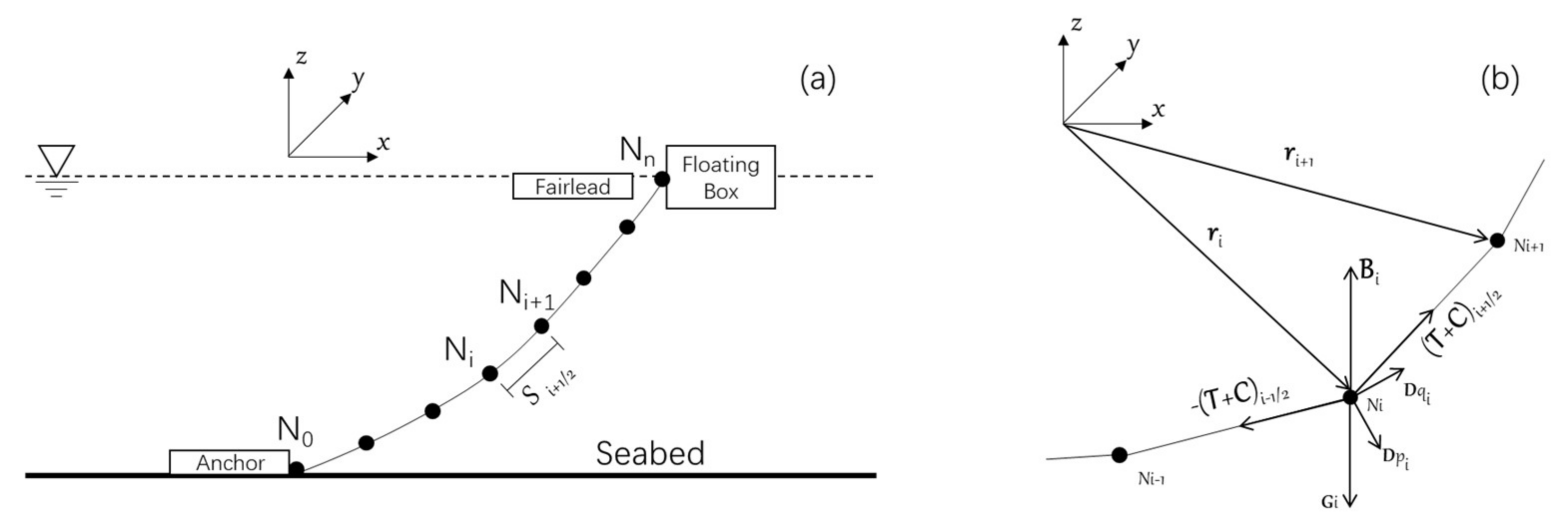
MoorDyn coupled with DualSPHysics was designed to use only the features needed to predict the dynamics of typical mooring systems. A floating box is moored using chains with an anchor and fairlead. The lumped-mass approach to cable dynamics is illustrated in Figure 1. The mooring cables are divided into N equally sized segments with N+1 nodes, as shown in Figure 1a. The anchor is set as node 0, and the fairlead as node Nn. The cable segment is numbered as Si + 1/2, which is between nodes i and i+1. Meanwhile, the forces on the node include the internal axial stiffness (T), damping forces (C), weight (G), buoyancy forces (B), hydrodynamic forces from Morison’s equation (D), and vertical spring–damper forces from contact with the seabed, as shown in Figure 1b. The acceleration of each node can be calculated by solving the equation as shown below. Finally, we can derive the resultant force (Fm) and torque (Tm) of the mooring system acting on the floating box. The complete motion equation for node i is:
Hall and Goupee [14] describe in detail MoorDyn’s capabilities for interconnected lines and elements in a mooring system.
3. Validation and Simulation
First, a 1-DoF decay case was simulated. Hence, numerical results for decay were validated against theoretical results, and numerical results for three-dimensional motion of a floating body were validated against the physical model data for tests carried out in [39]. Finally, SPH simulations of a floating body with moorings and without moorings were compared to examine the SPH-MoorDyn system.
3.1. Decay Test: Theory vs. SPH
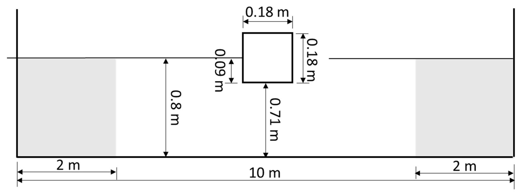
A decay test was carried out to validate the one-degree-of-freedom (1-DoF) simulation capacity of DualSPHysics. The theoretical results were the reference for the initial configuration of the SPH simulation, so the numerical tank was 10 m long and 1 m tall. The initial water level was 0.8 m. Damping areas that were 2 m long were set on both the left and right ends of the flume. In the middle of the flume, a floating box with an average density of 500 kg/m3 was half-immersed, and each side of the floating box was assumed to be 0.18 m. Figure 2 illustrates the numerical flume in the static equilibrium position. In this case, the initial particle spacing dp was 0.0025 m, leading to a smoothing length of 0.004243 m and 1,283,256 particles in 2-D.
Newton’s second law for a damped harmonic oscillator can be expressed as:
which can be rewritten in the form:
where is the angular frequency of the oscillator given by:
where is the displacement with respect to the equilibrium position; is the damping ratio, which critically determines the behaviors of the system; is the density of water; is the gravitational acceleration (9.81 m/s2); B is the dimension; is the added mass coefficient in the heave motion, which is equal to 0.9 according to experiments conducted on a half-immersed square floating box [39]; and M is the mass.
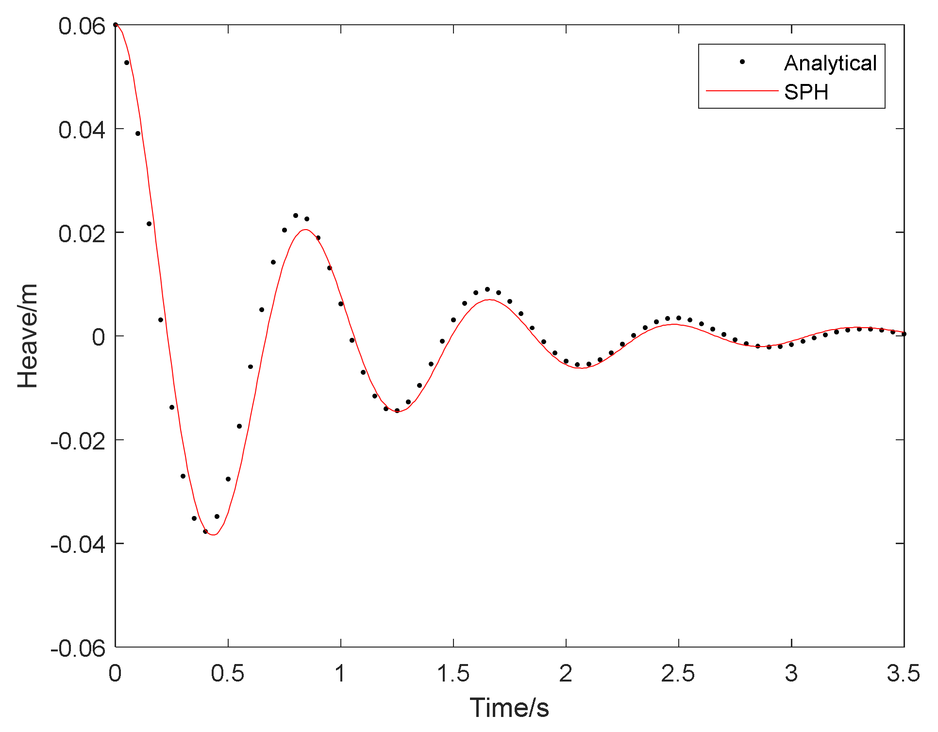
A decay test was then conducted. The initial displacement of the floating box was 0.06 m above the static equilibrium position. The damping ratio was 0.16. Figure 3 shows that DualSPHysics predicts the unique features of the theoretical model. The oscillation amplitude decreases following an exponentially underdamped system. We also observe that the oscillation frequencies of the SPH results gradually approach the analytic results, which indicates that DualSPHysics can be used to simulate the motions of a floating box.
The SPH heave amplitude is slightly overestimated compared with the analytical results. The choice of damping ratio and the complex fluid–solid interaction caused by the dynamic boundary conditions might have led to this discrepancy.
3.2. Floating Body Test: Experiment vs. SPH
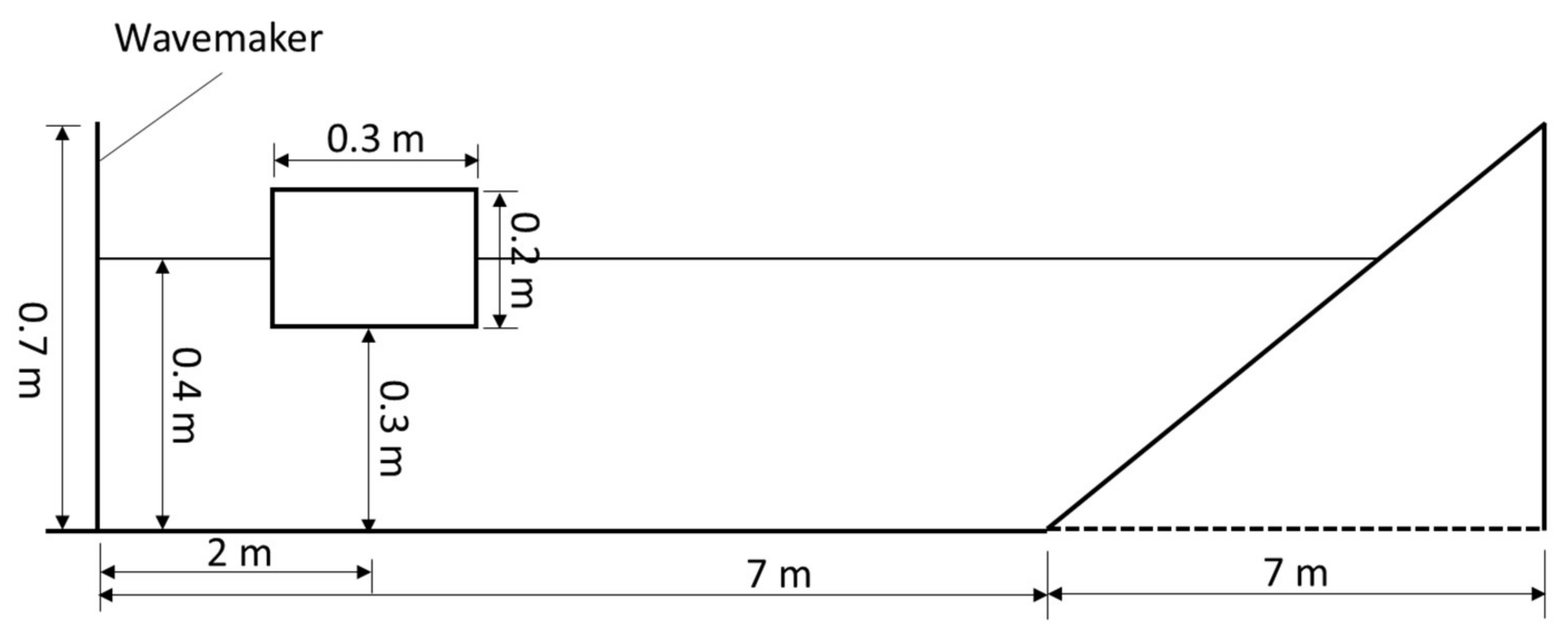
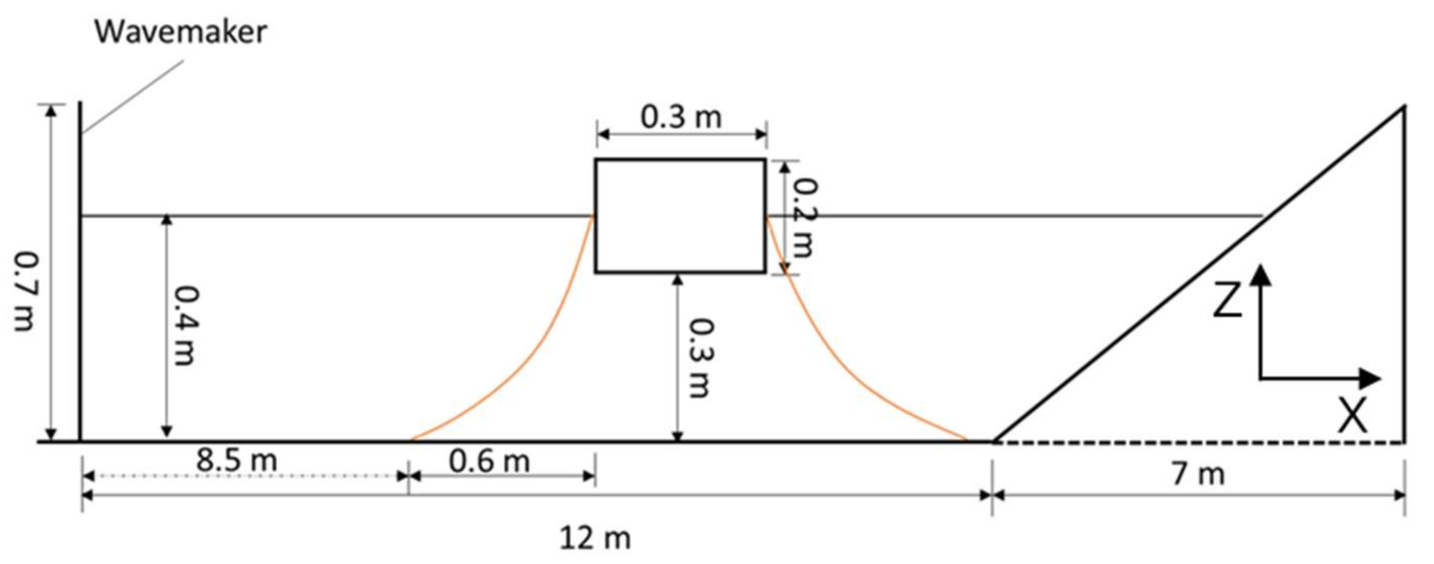
The numerical results for three-dimensional motion of a floating body were validated against the physical model test data in [40]. The experimental results are the reference for the initial configuration of the SPH simulation, so the numerical tank was 16 m long and 0.7 m tall. The initial water level was 0.4 m. A beach area that was 7 m long was set on the end of the numerical flume, while a piston-type wave generator was set on its left side. A rectangular body that was 0.3 m long and 0.2 m wide was located 2 m away from the wavemaker at the static equilibrium position. Figure 4 shows the initial state of the wave tank used to simulate the fluid–floating-box interaction. The experimental data (heave, surge, and pitch) included the time series of a freely floating box with three degrees of freedom (3-DoF). The box was 0.3 m long, 0.2 m high, and 0.42 m wide with a density of 500 kg/m3, resulting in a mass of 12.6 kg.
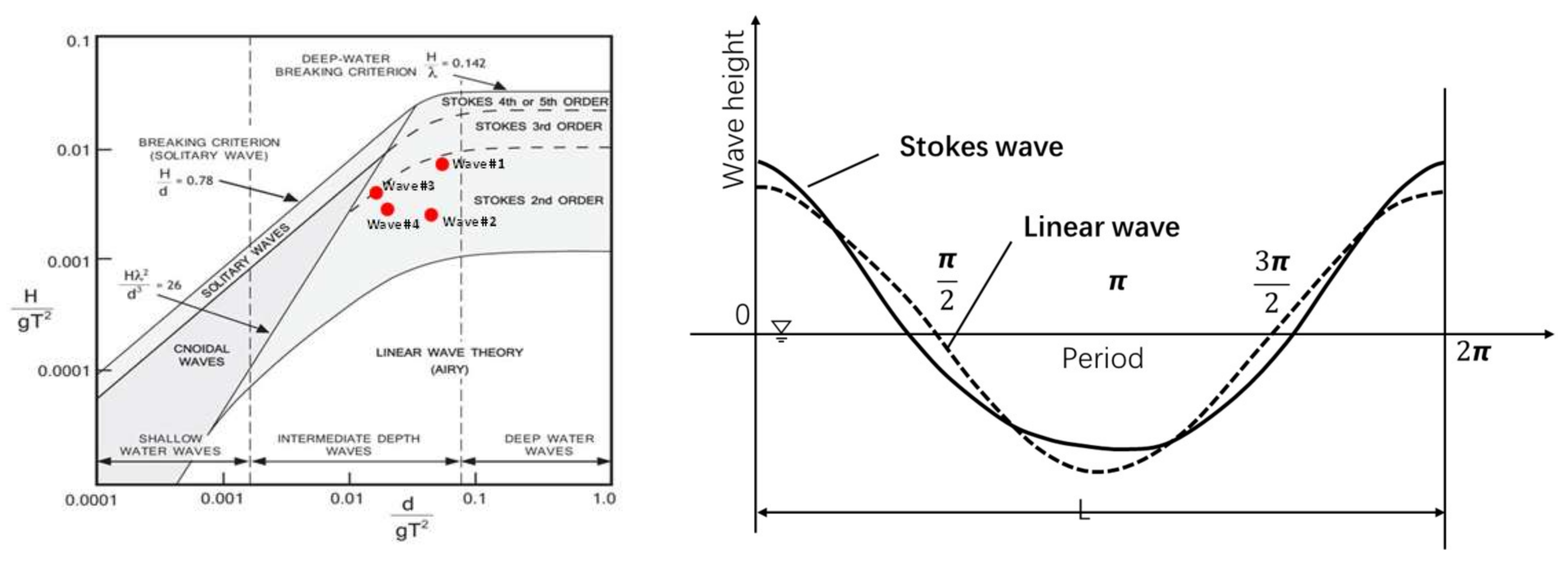
A regular wave with 0.1 m height and 1.2 s period was simulated according to Stokes second-order wave theory, because the wave had intermediate depths according to the values of the relative depth (d/L) (Figure 5).
An initial particle spacing (dp) of 0.005 m was selected, leading to a smoothing length equal to 0.00845 m in 2-D. The simulation was performed in 2-D to check this case. The 0.005 m initial particle distance leads to a total particle number of 124,544 in 2-D. The 2-D simulations took 53 min to simulate a 24 s physical process using a GeForce GTX 1070 Ti GPU card.
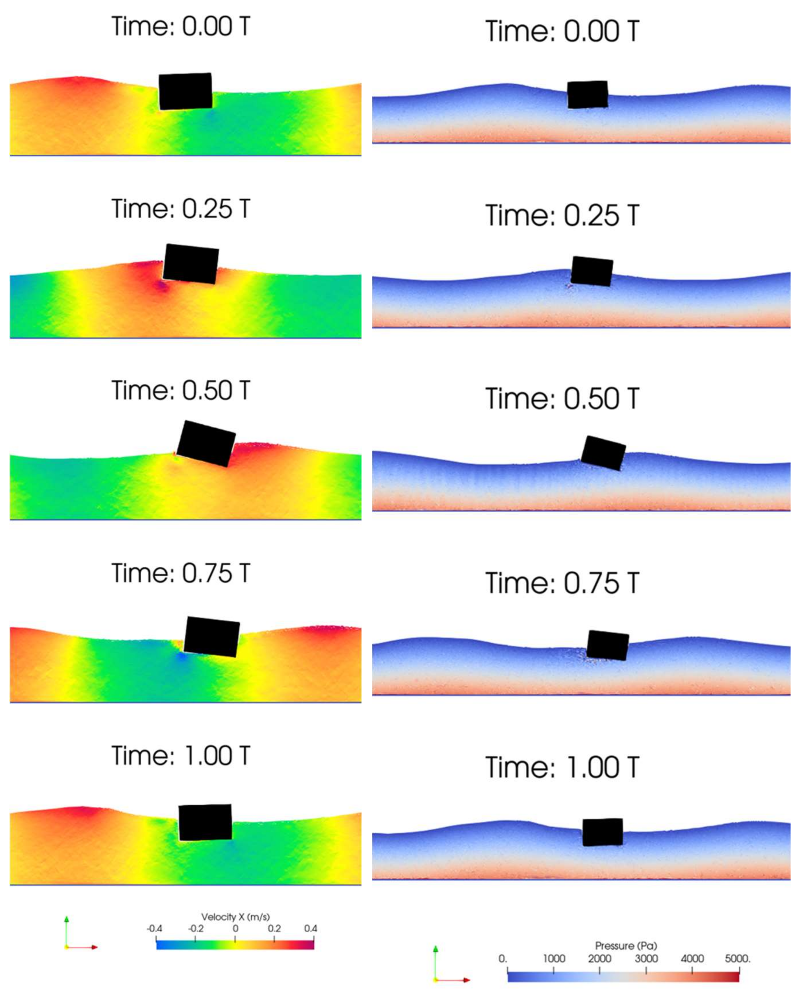
The picture on the left of Figure 6 shows snapshots of the horizontal flow velocity of the freely floating box under the regular wave, while the picture on the right of Figure 6 shows pressure snapshots of the freely floating box under the regular wave. The pitch angle can be observed over one full wave period. The first snapshot at time 0.00 T and the last snapshot at time 1.00 T show the same horizontal flow velocity field, the same pressure field, and the same pitch angle.
The picture on the left of Figure 6 shows snapshots of the horizontal flow velocity of the freely floating box under the regular wave, while the picture on the right of Figure 6 shows pressure snapshots of the freely floating box under the regular wave. The pitch angle can be observed over one full wave period. The first snapshot at time 0.00 T and the last snapshot at time 1.00 T show the same horizontal flow velocity field, the same pressure field, and the same pitch angle.
Figure 7 shows the comparison of the experimental and numerical time series of the 3-DoF motions under a regular wave with H = 0.1 m and T = 1.2 s. The experimental data [40] are compared with the DualSPHysics simulation results for dp = 0.005 m.
As we can see from Figure 7, the SPH motion trajectories agree well with the experimental data. The surge results present oscillations combined with drifting motions in the wave propagation direction due to the Stokes drift. The displacement of the drift was 0.1 m during this simulation. The drifting motions are driven by the mean drift force, which is proportional to the square of the sum of the reflected wave height and the scattered wave height [41], which obviously correlates with the incident wave height. The heave results show the floating box has been slightly elevated from the static equilibrium position and oscillates with the same period as the incident wave. The pitch results present oscillations too, and the floating box tilts forward at the beginning and then tilts backward, while the forward tilt angles are larger than the backward. The floating box is in a small forward tilt position compared with the static equilibrium position owing to the wave action. The rise of the centroid of the floating box and the forward tendency of the pitch angle could be explained by Stokes second-order wave theory (Figure 5). The intermediate-depth wave, which is the Stokes second-order wave here, has elevated sharp crests and elevated flat troughs. Furthermore, the crests and troughs are no longer symmetrical on the still-water surface owing to the nonlinear action, which leads to the rise of the centroid and a larger forward tilt angle.
All the results indicate that DualSPHysics can be used to simulate a fluid-driven object.
3.3. Floating Body Test: Mooring vs. without Mooring
Once the DualSPHysics fluid-driven object simulation was well checked to solve a comparable 2-D application (according to the good agreement in Figure 3 and Figure 7), MoorDyn was coupled with DualSPHysics to simulate the floating-body movements with mooring.
In this set of simulations, a floating body with mooring was investigated. Figure 8 shows the initial setup of the experiment with moorings. This experiment used the same configuration as in Figure 4 but with the rectangular center located 9.25 m away from the wavemaker. Moorings were set on both the left and right sides of the rectangular body; the mooring setup details are shown in Table 1. Experiments with and without moorings were conducted under a regular wave with H = 0.10 m, T = 1.2 s, and d = 0.4 m. The cables in the mooring system were divided into 20 equal segments, each with diameter D = 0.01 m and mass per unit length ml = 12 kg/m. A high cable stiffness, kcable = 4 × 10⁵ N/m, was used to avoid stretching of the mooring lines. The time step was Δtm = 1 × 10⁻⁴ s. To improve the computational efficiency, [1,20,41] developed codes for DualSPHysics with a CUDA toolkit using the GPU acceleration technique. The GPU card was an NVIDIA GeForce RTX 1070 Ti. The initial particle distance dp was 0.01, leading to a total particle number of 56,160. Simulating a 25 s physical process took 71,015 s.
Table 2 lists the locations of the fairleads on the floating box and anchors on the wave flume base. Here, x and z coordinate the distance from the wavemaker and depth. The initial position of the wavemaker is x = 0 while the initial water level presents z = 0. Mooring Line 1 (connecting Anchor 1 with Fairlead 1) is the front line with respect to the wave incidence direction, and Mooring Line 2 (connecting Anchor 2 with Fairlead 2) is the leeward-side rear line. In MoorDyn, the internal damping coefficient of the lines was selected automatically, leading to a damping ratio of 0.80 for each segment. Mass was added to the transverse direction with a coefficient set as 1.0. The coefficients for the transverse and axial directions were set as 1.6 and 0.05, respectively.
Because the floating box model was validated by the results in [40], a floating box with mooring was also simulated to correspond with the reference results. This simulation also had dp = 0.01 and 56,160 particles but took 1618 s to simulate a physical process of 25 s using the NVIDIA GeForce GTX 1070 Ti GPU card.
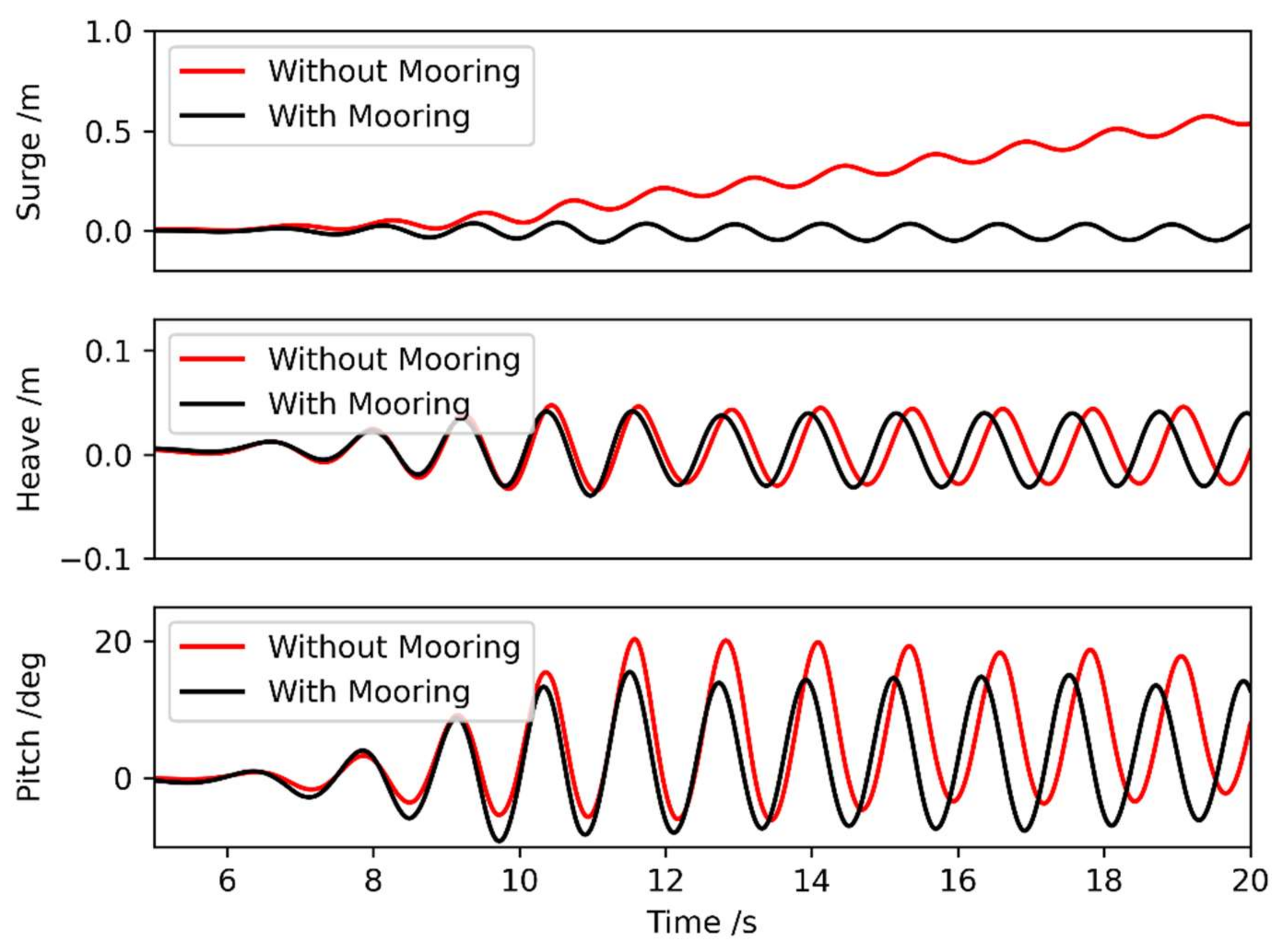
Figure 9 shows the simulation results for the surge, heave, and pitch of the floating box with and without mooring. The surge results show that the floating box drifted back and forth in the wave propagation direction with a displacement of 0.1 m, the freely floating box moved persistently along the wave propagation direction, and the box with mooring was not taken away by the wave motion because of the restriction from the mooring. The heave and pitch results show that, within a wave period, the floating box was lifted up and down with an amplitude of 0.04 m and pitched periodically with a range of 30°. The 3-DoF results show that the floating box with mooring had an advanced phase of motion compared with the freely floating box. Because the freely floating box was carried away by the waves, the waves acting on it propagated from the original position, which caused the motion of the floating box to be later than that of the moored one.
4. Application
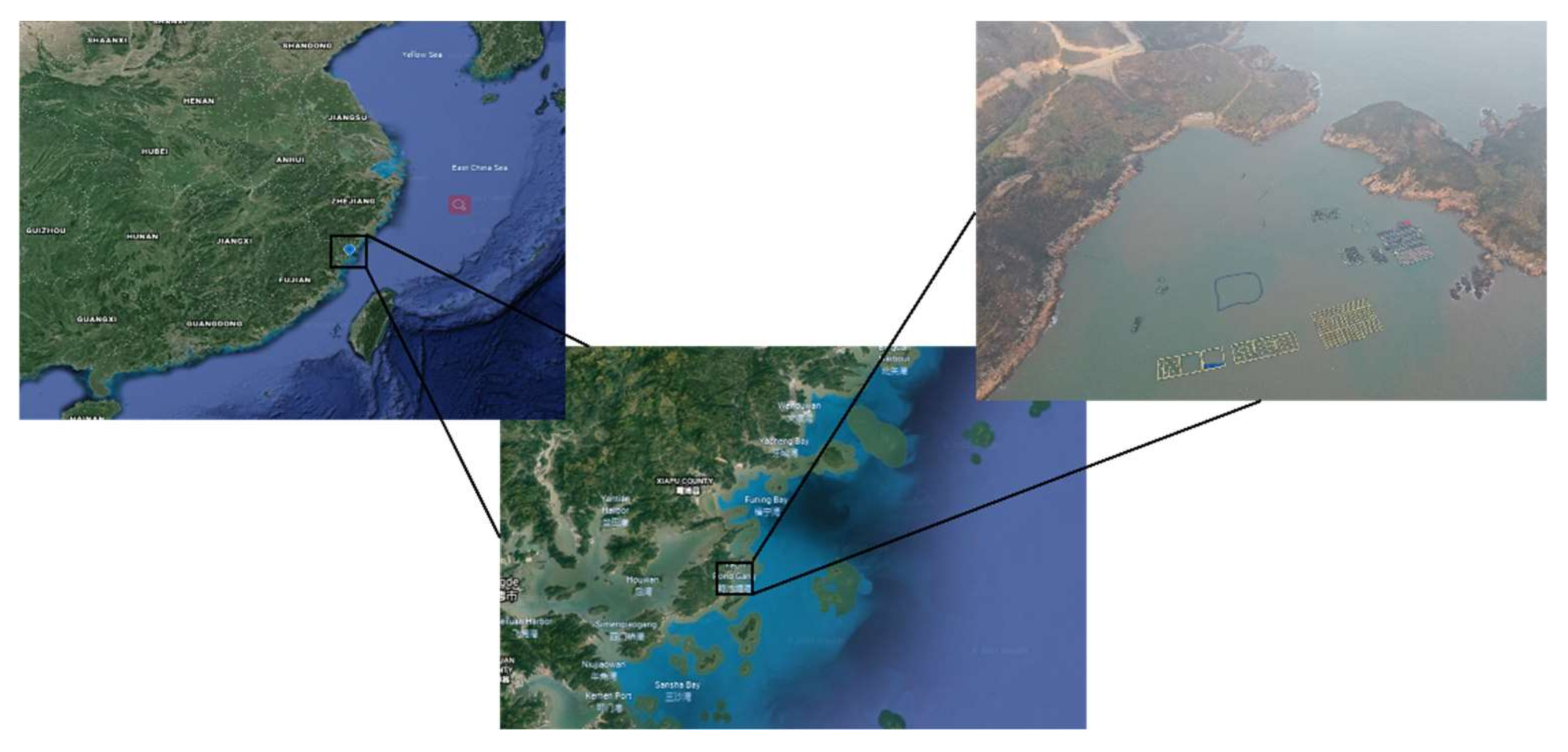
After a check that the solver is appropriate to solve a comparable 2-D application on solid–fluid interaction, it was used to study a real situation on the Chinese coast. A mariculture platform on the coast of Xiapu in China was studied here (Figure 10). The mariculture platform rears marine fish, large yellow croaker mostly, in cages suspended by floating rafts in coastal areas. The dimension of the cages ranges from a few meters to tens of meters, and the fishermen can walk and work on the floating frame. In this study, the 3-DoF motion of a large-scale mariculture platform with dimension of 20 m was simulated with realistic wave conditions by DualSPHysics.
The safety of fishermen and fish products should be highly valued in the mariculture platform. Regarding the safety of fishermen, according to the “Shallow Sea Mobile Platform Towing and Mooring Safety Regulations” [42] issued by the Chinese National Energy Administration, operations offshore need to be carried out when the wave height is less than 1 m. With reference to the safety guidelines for offshore floating platforms defined by Xie Guangci [43], the surge of the platform should not exceed 20% of the water depth, heave should not exceed 10% of the water depth, and the pitch angle under operating conditions should be less than 5°. Regarding the safety of fish products, we only consider the fish escape risks that may occur when the platform is submerged, tilted, and reversed in this work.
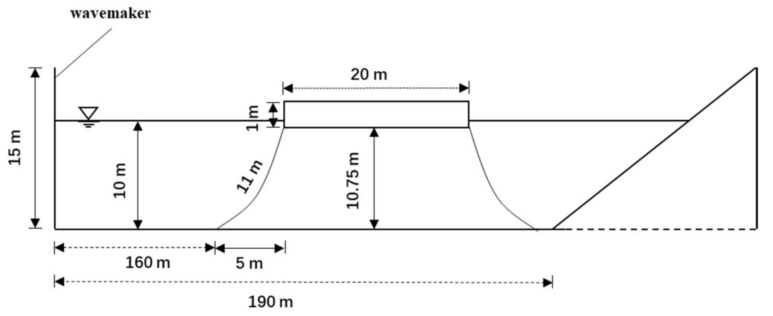
The following were the conditions of the initial setup of the numerical tank: (i) the simulation was 2-D for a section of the mariculture platform; (ii) proper wave generation and propagation was guaranteed because the tank was long enough; (iii) the dimensions used for the mariculture platform were the real ones; (iv) the regular waves were generated by a piston wavemaker using the measured wave heights and periods in that area. Figure 11 shows the numerical tank setup: the tank was 190 m in length, the piston wavemaker sat on the left side, the beach sat on the right side, the water depth was set as a realistic depth of this area, and the still-water depth was 10 m at the piston location.
The goal of this simulation was to mimic the 3-DoF motions of a simplified mariculture platform with two realistic wave conditions: a typical wave and a typhoon wave.
4.1. 3-DoF under a Typical Annual Wave
The typical annual wave was analyzed using the in situ buoy data, which show the real sea state of this area. The buoy is 18 km away from the mariculture platform and has been used to collect one year of wave data. The typical annual wave, which is the observed one-year significant wave height with a cumulative frequency of 75%, has a height of 0.6 m and period of 5 s. The regular and irregular waves were numerically reproduced. The waves had intermediate depths according to the values of the relative depth (d/L). Then, Stokes second-order wave theory was used to determine the wave kinematics of the test (Figure 5).
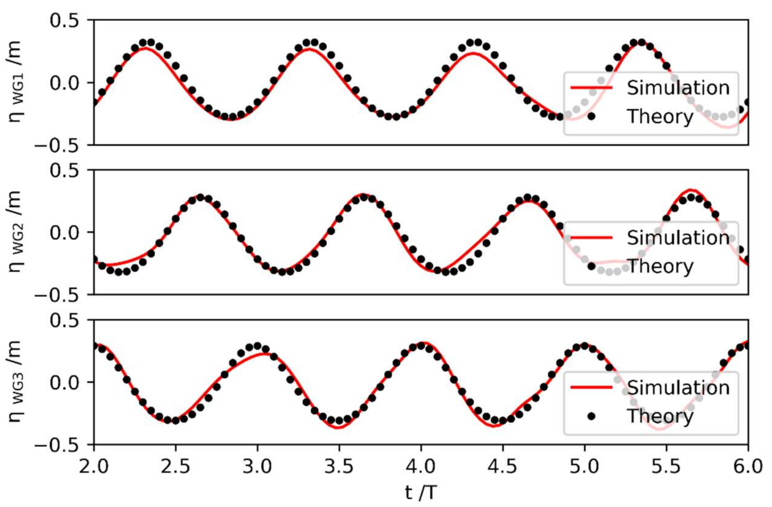
First, we validated the wave propagation obtained by comparing the numerical and theoretical values. The theoretical values were calculated using Stokes second-order wave theory. Figure 12 compares the theoretical and simulated surface elevations for a regular wave at WG1, WG2, and WG3 which is 10, 20, and 30 m from the wavemaker. The simulated SPH surface elevations follow Stokes second-order wave theory, demonstrating that waves are generated and propagated properly.
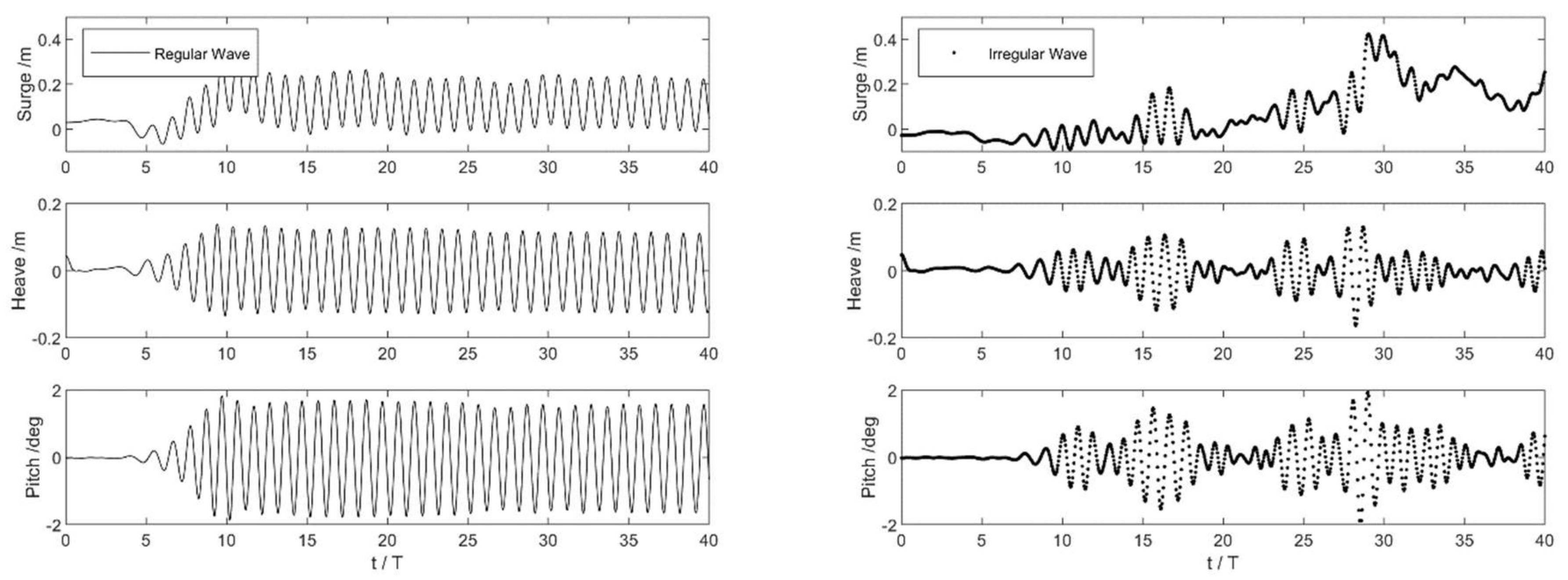
The waves generated and propagated by DualSPHysics have been proven accurate. The behavior of an open sea can be reproduced by a piston wavemaker in DualSPHysics, and the real sea state can also be mimicked. DualSPHysics can also be used to study the interaction between the waves and the mariculture platform on the coast of Xiapu. Therefore, DualSPHysics can be used to compute the 3-DoF motions of the mariculture platform. Figure 13 shows the simulated surge, heave, and pitch of the mariculture platform under the regular and irregular waves with H = 0.6 m and T = 5 s.
The experimental results for the regular wave reveal that the surge, heave, and pitch were steadily periodic after 15 wave periods. The surge results under the regular wave show that, within a wave period, the mariculture platform drifted back and forth in the wave propagation direction with a displacement of 0.22 m. The platform was not taken away by the wave with the restriction from moorings. The heave and pitch results for the regular wave show that, within a wave period, the mariculture platform was lifted up and down with an amplitude of 0.11 m and pitched periodically with a range of 3.4°.
The experimental results for the irregular wave show that the mariculture platform can be carried up to 0.42 m away from the original position, lifted up and down with an amplitude of 0.14 m, and pitched periodically with a range of 3.9°.
In this typical annual sea wave condition, the mariculture platform will not be rushed away or overturned. The fishermen are relatively safe if they stay and work on it, and the impact on fish activities in the cage is small. The design of the mariculture platform is appropriate.
4.2. 3-DoF under Typhoon Dujuan Waves
The coast of Xiapu in China endures high-frequency typhoon disasters. Typhoon Dujuan in 2015 landed 200 km away from this mariculture platform and caused extreme waves here. The maximum significant wave height recorded by the buoy, which is 18 km away from the mariculture platform, was 3.7 m with a period of 9.9 s. When the maximum significant wave height was present, the water level observed at the tidal gauge located 24 km away from the mariculture platform was 1.88 m. As we can see from Figure 14, the waves had intermediate depths, and the regular and irregular waves followed Stokes second-order wave theory. Therefore, the experiments were conducted under a regular wave and irregular wave with H = 3.7 m, T = 9.9 s, and a still-water depth set as d = 11.88 m. These experiments duplicated the most dangerous situations of the mariculture platform during Typhoon Dujuan.
Figure 14 shows the simulated surge, heave, and pitch of the mariculture platform under the regular and irregular waves with H = 3.7 m, T = 9.9 s, and a water level of 1.88 m.
The experimental results for the regular wave reveal that the heave and pitch have steady periodic motion after four wave periods. The mariculture platform drifted 2.5 m away from the original position even with the restriction from mooring, and drifted back and forth in the wave propagation direction with a displacement of 5.1 m. The mariculture platform was lifted up and down with an amplitude of 1.5 m and pitched periodically with a range of 14°.
The irregular-wave experimental results show that the mariculture platform can be carried up to 8.9 m away from the original position, lifted up and down with an amplitude of 1.6 m, and pitched periodically with a range of 20°.
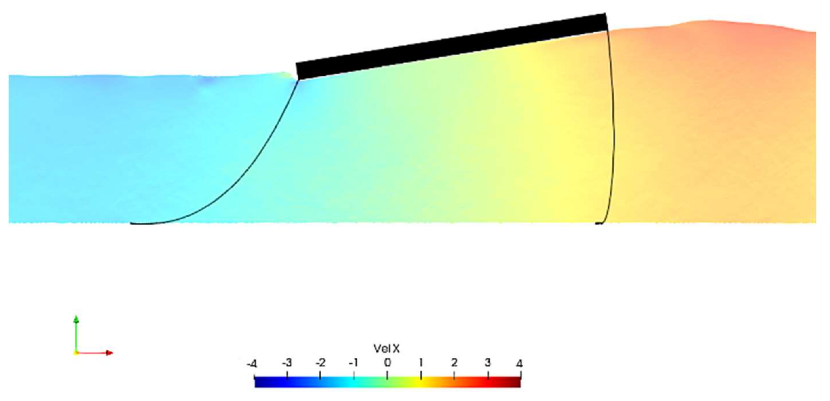
Figure 15 shows the snapshot of the mariculture platform with the largest pitch angle (9.18°) under the regular wave with H = 3.7 m and T = 9.9 s. The fish escape is likely occurring because of the platform tilts. Further, the escape might result in large property loss.
In this dangerous situation of extreme wave action, the mariculture platform experiences vigorous movement. It is not safe for the fishermen to stay and work, injuries from collision with fish and cages, and fish escapes may also occur.
To evaluate the impact of tidal water level variation on the hydrodynamic behavior of the mariculture platform, we conducted three experiments with different water levels. The experiments were designed on the basis of the wave and tidal level observations of the area adjacent to the mariculture platform. The mean high-tide level, mean tide level, and mean low-tide level were 3.64, 0.78, and −2.07 m, which were the levels observed at the nearest tidal gauge during the two days before Typhoon Dujuan landed. The average significant wave height, which was observed at the nearest buoy during the two days before Typhoon Dujuan landed, was 1.5 m.
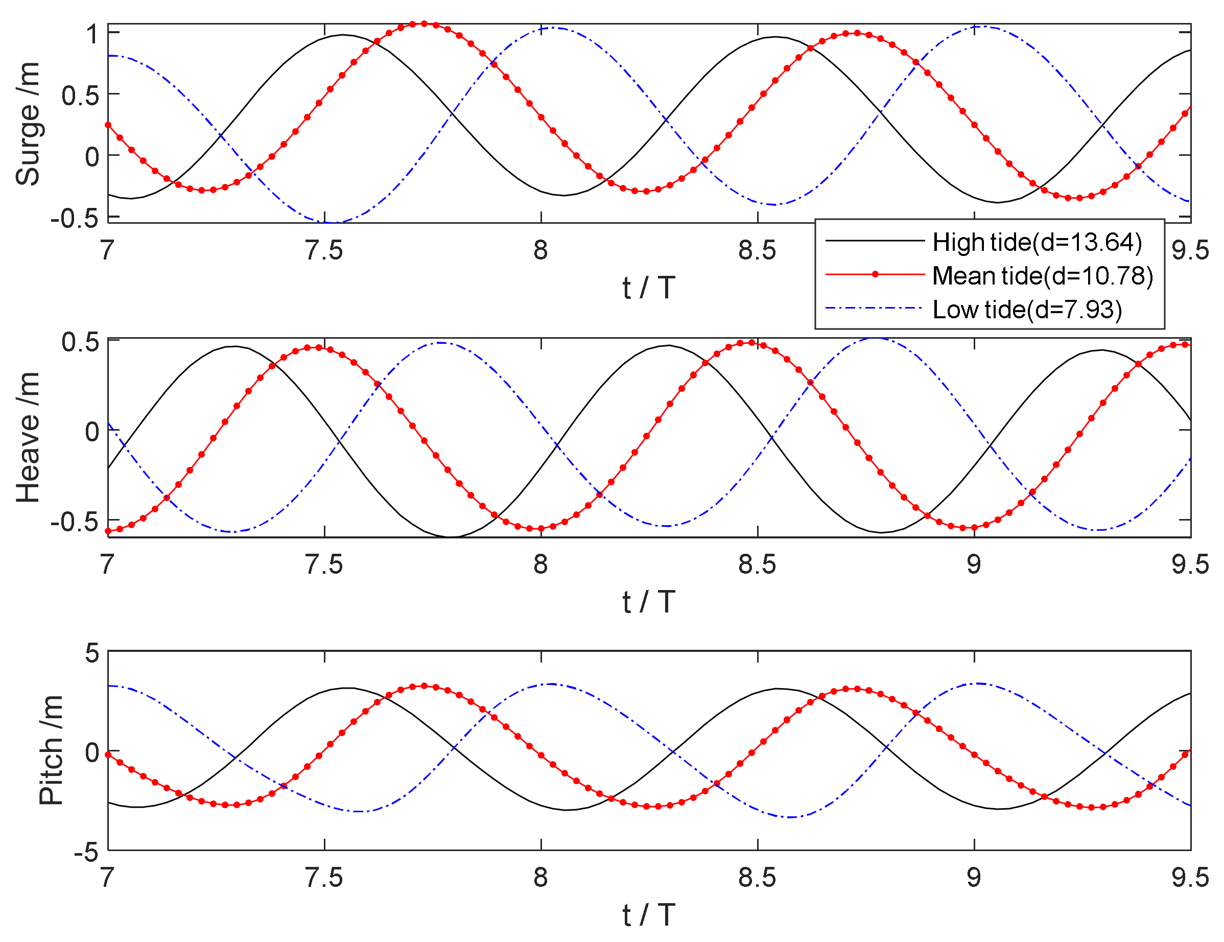
Then, the experiments were conducted under regular waves with H = 1.5 m and T = 7.4 s, and the still-water depth was set as d = 13.64 m, 10.78 m, and 7.93 m. The wave had intermediate depths, and the regular wave was determined by Stokes second-order wave theory (Figure 5). Figure 15 shows the simulated surge, heave, and pitch of the mariculture platform under the regular wave with H = 1.5 m and T = 7.4 s when the water level was 3.64, 0.78, and −2.07 m.
As we can see from Figure 16, the mariculture platform moved in advance, about half a period, with the increasing water depth under the same wave condition. The surge shrunk and the pitch angle decreased as the water depth grew. Ocean waves propagated in the intermediate-depth water, and the increasing water depth increased the wave propagation speed. This led the wave to be elongated and deformed, and the wave height decreased. As a result, there was an earlier motion response and smaller motion range.
In the average wave action of Typhoon Dujuan, the mariculture platform experiences vigorous movement. It is not safe for fishermen to stay and work, and injuries from collision with fish and cages may also occur. The analysis above reminds us that the fishermen should be evacuated, and the fish should be harvested or transferred before the typhoon arrives.
5. Conclusions
First, the DualSPHysics code was validated with a free decay test. The numerical results were compared with theoretical decay results. After that, a rectangular floating-structure test was performed with surge, heave, and pitch motions. The numerical results and experimental data were compared for a floating box, and good overall accuracy was achieved for the time series of surge, heave, and pitch. For the mooring simulation, MoorDyn was coupled with DualSPHysics. A 3-DoF comparison was made between a floating structure with moorings and one without moorings. The comparison shows that with the restriction from mooring, a floating box will not be taken away by the wave motion. The results reveal that DualSPHysics coupled with MoorDyn is an adaptive scheme that can simulate a fluid–solid–mooring system.
After the validation, the SPH code was used to study a Chinese coastal engineering case. The actual dimensions, bathymetry, and wave conditions of a mariculture platform were used in this study. The wave conditions were based on the nearest in situ buoy wave data, and the water level was based on the nearest tidal gauge observation. The 3-DoF behavior of the mariculture platform was simulated under a typical annual wave and a Typhoon Dujuan wave. The motion was light and gentle under the typical annual wave but vigorous under the Typhoon Dujuan wave. The results show that the design of this mariculture platform is appropriate for a typical annual wave, but the worker and aquaculture products should be well transferred before a typhoon arrives because of the vigorous movement under a typhoon wave. The motion response is earlier and the motion range smaller for a mariculture platform during a high tide. This work provides support to disaster warning, emergency evacuation, and engineering design.
Author Contributions
Conceptualization, S.S. and Y.X.; methodology, L.Z.; software, Z.W.; validation, F.Z., L.Z. and Z.W.; formal analysis, F.Z.; investigation, F.Z.; resources, Y.X.; data curation, Y.X.; writing—original draft preparation, F.Z.; writing—review and editing, L.Z.; visualization, S.S.; supervision, S.S.; project administration, S.S.; funding acquisition, S.S. and Y.X. All authors have read and agreed to the published version of the manuscript.
Funding
This work was jointly supported by the National Key R&D Program of China (Grant Nos. 2017YFC1404801 and 2016YFC1401104) Marine Economic Development Subsidy Project of Fujian, China (Grant No. ZHHY-2019-2) and Natural Science Project of Fujian Province, China (Grant No.2020J01860).
Acknowledgments
This work was jointly supported by the National Key R&D Program of China (Grant Nos. 2017YFC1404801 and 2016YFC1401104) Marine Economic Development Subsidy Project of Fujian, China (Grant No. ZHHY-2019-2) and Natural Science Project of Fujian Province, China (Grant No.2020J01860).
Conflicts of Interest
The authors declare no conflict of interest.
References
- Gabl, R.; Davey, T.; Nixon, E.; Steynor, J.; Ingram, D.M. Comparison of a floating cylinder with solid and water ballast. Water 2019, 11, 2487. [Google Scholar] [CrossRef] [Green Version]
- Gabl, R.; Davey, T.; Ingram, D.M. Roll motion of a water filled floating cylinder—Additional experimental verification. Water 2020, 12, 2219. [Google Scholar] [CrossRef]
- Palm, J.; Eskilsson, C.; Paredes, G.M. Coupled mooring analysis for floating wave energy converters using CFD: Formulation and validation. Int. J. Mar. Energy 2016, 16, 83–99. [Google Scholar] [CrossRef] [Green Version]
- Fernandes, C.; Semyonov, D.; Ferrás, L.L.; Nóbrega, J.M. Validation of the CFD-DPM solver DPMFoam in OpenFOAM® through analytical, numerical and experimental comparisons. Granul. Matter 2018, 20, 64. [Google Scholar] [CrossRef]
- Galuppo, W.; Magalhães, A.; Ferrás, L.L.; Nóbrega, J.M.; Fernandes, C. New boundary conditions for simulating the filling stage of the injection molding process. Eng. Comput. 2020, 38, 762–778. [Google Scholar] [CrossRef]
- Gu, H.; Peter, S.; Tim, S. Drag, added mass and radiation damping of oscillating vertical cylindrical bodies in heave and surge in still water. J. Fluids Struct. 2018, 82, 343–356. [Google Scholar] [CrossRef]
- Domínguez, J.M.; Crespo, A.J.C.; Hall, M.; Altomare, C.; Wu, M.; Stratigaki, V.; Troch, P.; Cappietti, L.; Gómez-Gesteira, M. SPH simulation of floating structures with moorings. Coast. Eng. 2019, 153, 103560. [Google Scholar] [CrossRef]
- Gonçalves, N.D.; Ferrás, L.L.; Carneiro, O.S.; Nóbrega, J.M. Using the GPU to design complex profile extrusion dies. Int. Polym. Process. 2015, 30, 442–450. [Google Scholar] [CrossRef] [Green Version]
- Domínguez, J.M.; Crespo, A.J.C.; Gómez-Gesteira, M. Optimization strategies for CPU and GPU implementations of a smoothed particle hydrodynamics method. Comput. Phys. Commun. 2013, 184, 617–627. [Google Scholar] [CrossRef]
- St-Germain, P.; Nistor, L.; Townsend, R. Smoothed-particle hydrodynamics numerical modeling of structures impacted by tsunami bores. J. Waterw. Port Coast. Ocean. Eng. 2014, 140, 66–81. [Google Scholar] [CrossRef]
- Zhang, F.; Crespo, A.; Altomare, C. DuaISPHysics: A numerical tool to simulate real breakwaters. J. Hydrodyn. 2018, 30, 95–105. [Google Scholar] [CrossRef]
- Canelas, R.B.; Domínguez, J.M.; Crespo, A.J.C. A smooth particle hydrodynamics discretization for the modelling of free surface flows and rigid body dynamics. Int. J. Numer. Methods Fluids 2015, 78, 581–593. [Google Scholar] [CrossRef]
- Altomare, C.; Domínguez, J.M.; Crespo, A.J.C.; González-Cao, J.; Suzuki, T.; Gómez-Gesteira, M.; Troch, P. Long-crested wave generation and absorption for SPH-based DualSPHysics model. Coast. Eng. 2017, 127, 37–54. [Google Scholar] [CrossRef]
- Hall, M.; Goupee, A. Validation of a lumped-mass mooring line model with DeepCwind semisubmersible model test data. Ocean. Eng. 2015, 104, 590–603. [Google Scholar] [CrossRef] [Green Version]
- Vissio, G.; Passione, B.; Hall, M. Expanding ISWEC modelling with a lumped-mass mooring line model. In Proceedings of the European Wave and Tidal Energy Conference, Nantes, France, 6–11 September 2015. [Google Scholar]
- Hall, M. Efficient modelling of seabed friction and multi-floater mooring systems in MoorDyn. In Proceedings of the 12th European Wave and Tidal Energy Conference, Cork, Ireland, 27 August–1 September 2017. [Google Scholar]
- Lee, S.C.; Song, S.; Park, S. Platform motions and mooring system coupled solver for a moored floating platform in a wave. Processes 2021, 9, 1393. [Google Scholar] [CrossRef]
- Quartier, N.; Ropero-Giralda, P.; Domínguez, M.J.; Stratigaki, V.; Troch, P. Influence of the drag force on the average absorbed power of heaving wave energy converters using smoothed particle hydrodynamics. Water 2021, 13, 384. [Google Scholar] [CrossRef]
- Pribadi, A.B.K.; Donatini, L.; Lataire, E. Numerical modelling of a mussel line system by means of lumped-mass approach. J. Mar. Sci. Eng. 2019, 7, 309. [Google Scholar] [CrossRef] [Green Version]
- Crespo, A.J.C.; Domínguez, J.M.; Rogers, B.D.; Gómez-Gesteira, M.; Longshaw, S.; Canelas, R.; Vacondio, R.; Barreiro, A.; García-Feal, O. DualSPHysics: Open-source parallel CFD solver on SPH. Comput. Phys. Commun. 2015, 187, 204–216. [Google Scholar] [CrossRef]
- Domínguez, J.M.; Crespo, A.J.C.; Valdez-Balderas, D.; Rogers, B.D.; Gómez-Gesteira, M. New multi-GPU implementation for smoothed particle hydrodynamics on heterogeneous clusters. Comput. Phys. Commun. 2013, 184, 1848–1860. [Google Scholar] [CrossRef]
- Crespo, A.J.C.; Domínguez, J.M.; Barreiro, A.; Gómez-Gesteira, M.; Rogers, B.D. GPUs, a new tool of acceleration in CFD: Efficiency and reliability on Smoothed Particle Hydrodynamics methods. PLoS ONE 2011, 6, e20685. [Google Scholar] [CrossRef]
- Altomare, C.; Crespo, A.J.C.; Rogers, B.D.; Dominguez, J.M.; Gironella, X.; Gómez-Gesteira, M. Numerical modelling of armour block sea breakwater with smoothed particle hydrodynamics. Comput. Struct. 2014, 130, 34–45. [Google Scholar] [CrossRef]
- Altomare, C.; Crespo, A.J.C.; Domínguez, J.M.; Gómez-Gesteira, M.; Suzuki, T.; Verwaest, T. Applicability of smoothed particle hydrodynamics for estimation of sea wave impact on coastal structures. Coast. Eng. 2015, 96, 1–12. [Google Scholar] [CrossRef]
- Liu, G.R.; Liu, M.B. Smoothed Particle Hydrodynamics: A Meshfree Particle Method; World Scientific: Singapore, 2003. [Google Scholar]
- Wendland, H. Piecewiese polynomial, positive definite and compactly supported radial functions of minimal degree. Adv. Comput. Math. 1995, 4, 389–396. [Google Scholar] [CrossRef]
- Monaghan, J.J. Smoothed particle hydrodynamics. Annu. Rev. Astron. Astrophys. 1992, 30, 543–574. [Google Scholar] [CrossRef]
- Monaghan, J.J.; Cas, R.A.F.; Kos, A.M.; Hallworth, M. Gravity currents descending a ramp in a stratified tank. J. Fluid Mech. 1999, 379, 39–70. [Google Scholar] [CrossRef]
- Verlet, L. Computer experiments on classical fluids. I. Thermodynamical properties of Lennard-Jones molecules. Phys. Rev. 1967, 159, 98–103. [Google Scholar] [CrossRef]
- Leimkuhler, B.J.; Reich, S.; Skeel, R.D. Integration methods for molecular dynamics. In Mathematical Approaches to Biomolecular Structure and Dynamics; The IMA Volumes in Mathematics and Its Applications; Mesirov, J.P., Schulten, K., Sumners, D.W., Eds.; Springer: New York, NY, USA, 1996; Volume 82. [Google Scholar]
- Batchelor, G.K. Introduction to Fluid Dynamics; Cambridge University Press: Cambridge, UK, 1974. [Google Scholar]
- Leimkuhler, B.J.; Reich, S.; Skeel, R.D. Integration methods for molecular dynamic. In the IMA Volume in Mathematics and Its Application; Springer: New York, USA, 1996. [Google Scholar]
- Crespo, A.J.C.; Gómez-Gesteira, M.; Dalrymple, R. Boundary conditions generated by dynamic particles in SPH Methods. Comput. Mater. Contin. 2007, 5, 173–184. [Google Scholar]
- Domínguez, J.M.; Crespo, A.J.C.; Cercós-Pita, J.L.; Fourtakas, G.; Rogers, B.D.; Vacondio, R. Evaluation of reliability and efficiency of different boundary conditions in an SPH code. In Proceedings of the 10th SPHERIC International Workshop, Parma, Italy, 9 June 2015. [Google Scholar]
- Biesel, F.; Suquet, F. Etude theorique d’un type d’appareil a la houle. LaHouille Blanche 1951, 2, 157–160. [Google Scholar]
- Madsen, O.S. On the generation of long waves. J. Geophys. Res. 1971, 76, 8672–8683. [Google Scholar] [CrossRef]
- Schäffer, H.A.; Klopman, G. Review of multidirectional active wave absorption methods. J. Waterw. Port Coast. Ocean. Eng. 2000, 126, 88–97. [Google Scholar] [CrossRef]
- Dalrymple, R.A.; Dean, R.G. Water Wave Mechanics for Engineers and Scientists; World Scientific Publishing Company: Singapore, 1991. [Google Scholar]
- Cen, Y. Study on Operating Characteristics of Oscillating-Buoy Wave Energy Converter. Ph.D. Thesis, Tsinghua University, Beijing, China, 2015. [Google Scholar]
- Ren, B.; He, M.; Dong, P.; Wen, H. Nonlinear simulations of wave-induced motions of a freely floating body using WCSPH method. Appl. Ocean Res 2015, 50, 1–12. [Google Scholar] [CrossRef]
- Mauro, H. The drift of a body floating on waves. J. Ship Res. 1960, 4, 1–10. [Google Scholar]
- National Energy Administration of China. Shallow Sea Mobile Platform Towing and Mooring Safety Specification[S]; National Energy Administration of China: Beijing, China, 2016.
- Xie, G. Conceptual Design of Offshore Wind-Wave Combined Power Generation Platform. Ph.D. Thesis, Harbin Engineering University, Harbin, China, 2020. [Google Scholar]
Figure 1.
Illustration of the lumped-mass approach: (a) mooring line discretization; (b) internal and external forces on a cable.
Figure 1.
Illustration of the lumped-mass approach: (a) mooring line discretization; (b) internal and external forces on a cable.

Figure 2.
Illustration of the wave tank used in the decay test.

Figure 3.
Comparison of the analytical and numerical heaves for the decay test.

Figure 4.
Wave tank used to simulate the fluid–floating-box interaction.

Figure 5.
Scope of wave theory. (Floating Body Test Wave #1 with H = 0.1 m T = 1.2 s; Typical annual wave simulation Wave#2 with H = 0.6m T = 5 s; Typhoon Dujuan simulation Wave#3 with H = 3.7 m T = 9.9 s; Typhoon experiments Wave#4 with H = 1.5 m, T = 7.4 s).
Figure 5.
Scope of wave theory. (Floating Body Test Wave #1 with H = 0.1 m T = 1.2 s; Typical annual wave simulation Wave#2 with H = 0.6m T = 5 s; Typhoon Dujuan simulation Wave#3 with H = 3.7 m T = 9.9 s; Typhoon experiments Wave#4 with H = 1.5 m, T = 7.4 s).

Figure 6.
Different snapshots of the freely floating box under regular waves. Particle colors correspond to the horizontal flow velocity (left) and pressure (right) values.
Figure 6.
Different snapshots of the freely floating box under regular waves. Particle colors correspond to the horizontal flow velocity (left) and pressure (right) values.

Figure 7.
Comparison between experimental and numerical time series of the 3-DoF motions under a regular wave with H = 0.1 m and T = 1.2 s.
Figure 7.
Comparison between experimental and numerical time series of the 3-DoF motions under a regular wave with H = 0.1 m and T = 1.2 s.

Figure 8.
Initial setup of the floating-body experiment with mooring.

Figure 9.
Comparison of the 3-DoF motions for wave #1 with and without mooring.

Figure 10.
Picture of the mariculture platform on the coast of Xiapu.

Figure 11.
Initial setup of the application case.

Figure 12.
Comparison between theoretical and numerical surface elevations under a regular wave with H = 0.6 m and T = 5 s.
Figure 12.
Comparison between theoretical and numerical surface elevations under a regular wave with H = 0.6 m and T = 5 s.

Figure 13.
Time series of 3-DoF motions of the mariculture platform under the regular and irregular waves with H = 0.6 m and T = 5 s simulated with SPH.
Figure 13.
Time series of 3-DoF motions of the mariculture platform under the regular and irregular waves with H = 0.6 m and T = 5 s simulated with SPH.

Figure 14.
Time series of 3-DoF motions of the mariculture platform under the regular and irregular waves with H = 3.7 m, T = 9.9 s, and d = 11.88 m simulated with SPH.
Figure 14.
Time series of 3-DoF motions of the mariculture platform under the regular and irregular waves with H = 3.7 m, T = 9.9 s, and d = 11.88 m simulated with SPH.

Figure 15.
Snapshot of the mariculture platform with H = 3.7 m, T = 9.9 s, and d = 11.88 m simulated with SPH. Particle colors correspond to the horizontal flow velocity.
Figure 15.
Snapshot of the mariculture platform with H = 3.7 m, T = 9.9 s, and d = 11.88 m simulated with SPH. Particle colors correspond to the horizontal flow velocity.

Figure 16.
Time series of 3-DoF motions of the mariculture platform under the regular wave with H = 1.5 m, T = 7.4 s, and d = 13.64 m, 10.78 m, and 7.93 m simulated with SPH.
Figure 16.
Time series of 3-DoF motions of the mariculture platform under the regular wave with H = 1.5 m, T = 7.4 s, and d = 13.64 m, 10.78 m, and 7.93 m simulated with SPH.


Table 1.
Moordyn setup.
| Time step size | 1 × 10⁻⁴ s |
| Segments | 20 |
| Diameter | 0.01 m |
| Mass per unit length | 12 kg/m |
| Cable stiffness | 4 × 10⁵ N/m |
Table 2.
Locations of the fairleads and anchor points.
| Points | Coordinates (x, z) |
|---|---|
| Anchor 1 | (8.5, −0.4) |
| Fairlead 1 | (9.1, 0.0) |
| Anchor 2 | (10, −0.4) |
| Fairlead 2 | (9.4, 0.0) |
Publisher’s Note: MDPI stays neutral with regard to jurisdictional claims in published maps and institutional affiliations. |
© 2021 by the authors. Licensee MDPI, Basel, Switzerland. This article is an open access article distributed under the terms and conditions of the Creative Commons Attribution (CC BY) license (https://creativecommons.org/licenses/by/4.0/).
Share and Cite
MDPI and ACS Style
Zhang, F.; Zhang, L.; Xie, Y.; Wang, Z.; Shang, S. Smoothed Particle Hydrodynamics Simulation of a Mariculture Platform under Waves. Water 2021, 13, 2847. https://doi.org/10.3390/w13202847
AMA Style
Zhang F, Zhang L, Xie Y, Wang Z, Shang S. Smoothed Particle Hydrodynamics Simulation of a Mariculture Platform under Waves. Water. 2021; 13(20):2847. https://doi.org/10.3390/w13202847
Chicago/Turabian StyleZhang, Feng, Li Zhang, Yanshuang Xie, Zhiyuan Wang, and Shaoping Shang. 2021. "Smoothed Particle Hydrodynamics Simulation of a Mariculture Platform under Waves" Water 13, no. 20: 2847. https://doi.org/10.3390/w13202847
Note that from the first issue of 2016, this journal uses article numbers instead of page numbers. See further details here.