The Use of High-Speed Cameras as a Tool for the Characterization of Raindrops in Splash Laboratory Studies

Abstract

Measuring the characteristics of raindrops is essential for different processes studies. There have been many methods used throughout history to measure raindrops. In recent years, automatic image recognition and processing systems have been used with high-speed cameras to characterize rainfall by obtaining the spectrum of droplet sizes and their speeds and thus being able to use this technology to calibrate rainfall simulators. In this work, two phases were carried out: in the first one, individual drops with terminal speeds of different sizes were measured and processed both in speed and in shape with a high-speed camera; and in the second phase, a calibration procedure was designed but in multidrop images, determining the characteristics of the drops produced by a rain simulator. According to results, the real shape of each drop depending on the size was determined, from round to ovaloid shapes, and the terminal velocity of water drops with different sizes was measured. Based on the rain images used to calibrate a rainfall simulator, it was observed that, with a higher intensity of rain, the drops produced were smaller, which contrasts with real rain, in which just the opposite happens. This calibration evaluates their resemblance to reality, calculates the real kinetic energy of the rain they produce and see if they can be used to model events in nature.

1. Introduction

Measuring the characteristics of raindrops is essential for different processes and recently has attracted increased attention of meteorological research worldwide [1]. It is well known that the size of the raindrops is related to the capacity of the rainfall to clean the atmosphere of aerosols [2,3], and it also has an influence in the attenuation of radio waves [4,5,6], changing the propagating radio frequency. There are other important applications for the determination of drop-size distributions (DSD), some more related with human health, such as the influence in cancer of lung, allergies or other problems [7], and other more related with planet health, such as the influences in herbicides application [8,9] or the analysis of the splash erosion effects [10,11]. Indeed, this last topic is receiving a lot of scientific attention due to the great importance of water as a main erosive agent for the soil [12].

Splash erosion occurs at the initial stages of soil water erosion [13,14,15,16]. The first stage of water erosion is the splash phenomenon, when raindrops falling on the soil surface cause the loosening and ejection of soil particles, which are displaced over different distances [17,18]. Splash erosion is directly related to the breakdown of soil aggregates [8,9,19,20,21], the enhancement of aggregates dispersion and transport [22,23,24,25,26], and surface crusting [27], resulting in changes to soil infiltration parameters [28]. It should be noted that the effects of splash also contribute to the transportation of microorganisms [29,30] and pollutants [31], along with the ejected particles.

The capacity of splash effects, including the displaced mass [32,33] and analysis of distances over which particles are ejected [34,35,36], has been determined by the different drop-size distributions, which control the kinetic energy of the impacts of raindrops on soil [20,37]. The rainfall characteristics such as rainfall kinetic energy [38,39,40], intensity [41] and raindrop diameter [21,42,43] have been assessed. In fact, the determination of the size of the drops has been one of the parameters that has attracted the most attention of many researchers due to the errors that can originate in the estimates of the rest of the characteristics [20].

There have been many methods used throughout history to measure raindrops: from the most precarious, such as using containers with flour exposed for a short and defined time to rain [44] in which the drops fell and became small stones of dry flour with which they could know the size of these drops, or the use of absorbent papers or covered fabrics [45] with soluble paints on which the drops fell, thus being able to measure their sizes reflected in the spots on the paper. This last system can also be organized with dry invisible ink that reacts on contact with water, leaving with each drop a circular spot related to its size that can be measured later. To calculate the size of the drop the following formula is used: D = a × S × b, with D the diameter of the drop, S the diameter of the stained spot, and constants a and b that are established by calibrating the used paper in the laboratory [45].

More recently, more complex methodologies have been developed, such as using a wind tunnel to be able to measure the terminal velocity of the drops and see their behavior during their fall [46], or the use of disdrometers, which are specialized instruments for measuring drops. Two types of disdrometers exist: the optical disdrometers [47,48], which measure droplet sizes by measuring interruptions produced by water droplets in a wave emission, or impact disdrometers [49,50], which consist of a sensor that transforms the moment associated with the impact of the drop into an electrical pulse, whose amplitude is a function of the diameter of the drop.

Today, the most widely used are optical disdrometers [47,51], consisting of a transmitter and a laser receiver, which are exposed to the air. When it rains, the drops pass through the laser beam, and the instrument registers with each drop a decrease in the power of the transmitter, which is proportional to the size of these drops since they allow the use of different wavelengths to evaluate the distribution of the size of the drops, as well as their speed and shape. Besides that, they allow the kinetic energy of these drops to be determined—one of the most relevant parameters in water erosion studies.

However, in addition to the instruments named so far, in the age of the image, we cannot forget the possibilities of integrating photography and automatic image recognition and processing systems, which are ways to improve the possibilities of determining sizes of drops and their velocities. In fact, in recent years, some work has been carried out with high-speed cameras to characterize rainfall by obtaining the spectrum of droplet sizes and their speed and thus be able to use this technology to calibrate rainfall simulators. This method has new and high potential, such as the evaluation of the influence of the wind on the formation of the drops; the determination of animal pollen or other objects in the sampling area; or the determination of the influence of the oscillations of any drop. However, it also implies great difficulties when using this method for the determination of speed and size, such as the need to carry out preliminary calibrations of the devices because they are not specific for this purpose, the requirement of robust computer programs that allow performing the treatments of the photos, the need for correct lighting to avoid drops that are not detected, the shadows of the raindrops, and, of course, the need to control the background by using different focus planes. If these errors are not taken into account, there could be different depths in the image, leading to distant drops that are confused with smaller drops or nearby drops that appear larger than they really are. Therefore, it is necessary to calibrate, which means working with patterns that must be made from drops of known sizes that are launched from known heights, in order to determine both the speed they reach and what shape and how they are detected by the camera. Speed calibration has not been carried out up to now, due to its difficulty, and is usually solved by applying the theoretical model of Gunn and Kinzer [52], which only serves to work with very controlled situations and without the influence of wind currents. Therefore, the theoretical exponential and gamma relations of the Marshall and Palmer droplet size distributions [53] and Gunn and Kinzer terminal velocities models [52] cannot represent the situations of all the natural precipitations that take place, much less of the existing rainfall simulators. This is why it is necessary to establish a methodology that defines the complete calibration procedure for the use of a high-speed camera to determine the sizes of the water droplets and velocity. To be able to carry it out, in this work the tasks have been divided into two phases: in the first phase, individual drops were produced to reach terminal speeds of different sizes and were measured and processed both in speed and in shape with a high-speed camera. In the second phase, the knowledge determined in the first part was applied to design a calibration procedure for multidrop images, determining the characteristics of the drops produced by a rainfall simulator (the spectra of the number of drops per minute according to the different sizes, at different simulated rainfall intensities) through the systematic taking of photographs and the use of software for their characterization.

2. Materials and Methods

2.1. Materials

For the initial experiments, two high-speed cameras were used: a Smart High-Speed Camera ProcImage250 (Monochrome version) and a FASTCAM-APX RS model 250K that allowed taking pictures under water.

The Smart High-Speed Camera has a resolution of 640 × 480 pixels, 252 frames per second (fps) at full resolution and up to 54,000 fps, ROI configurable in size and position, and I/O connector: trigger input, sync input/output, strobe output. The camera was controlled by EyeMotion software.

The “FASTCAM-APX RS model 250K” camera which has the following specifications: Global electronic shutter up to 2 μs, camera control interface: High-Speed Gigabit Ethernet, National Instruments DAQ support, Photron FASTCAM Viewer: simple and easy-to-control software for Ultima camera, Photron FASTCAM Analysis (PFA): entry-level analysis software for displacement, velocity, and acceleration measurements. This camera configuration used was: definition 256 × 256, 563.4 fps, exposure 40.1 µs. After taking the average of the thirty measurements taken, the following equivalence was achieved: 10 mm = 30.6102 pixels SD.

A metal tripod was used to hold the cameras, with which the appropriate height for the camera was adjusted. In addition, a photography focus with a continuous light source was used, widely used when performing studies of this type: 800 W tungsten lamp, 3200 K color temperature with adjustable visors to direct the light (16 × 17 cm). A screen was added to the spotlight to achieve a homogeneous light background to facilitate measurements.

For the treatment of the images with a few drops (individual or with a maximum of 5 drops), the free program ImageJ was used, which is a digital image processing program, programmed in Java and developed at the National Institutes of Health [54]. It was designed with an open architecture that provides extensibility via plugins and macros that allow solving various image processing and analysis problems and developing a custom image scan, among other things.

For the treatment of the multidrop images, the MATLAB program is used to process and treat different files such as images; for this reason, it was decided upon to use this program to carry out the analysis of the images collected by the camera. MATLAB program is able to modify images pixel by pixel, which allows the process to be automated and thus treat thousands of images in a short time.

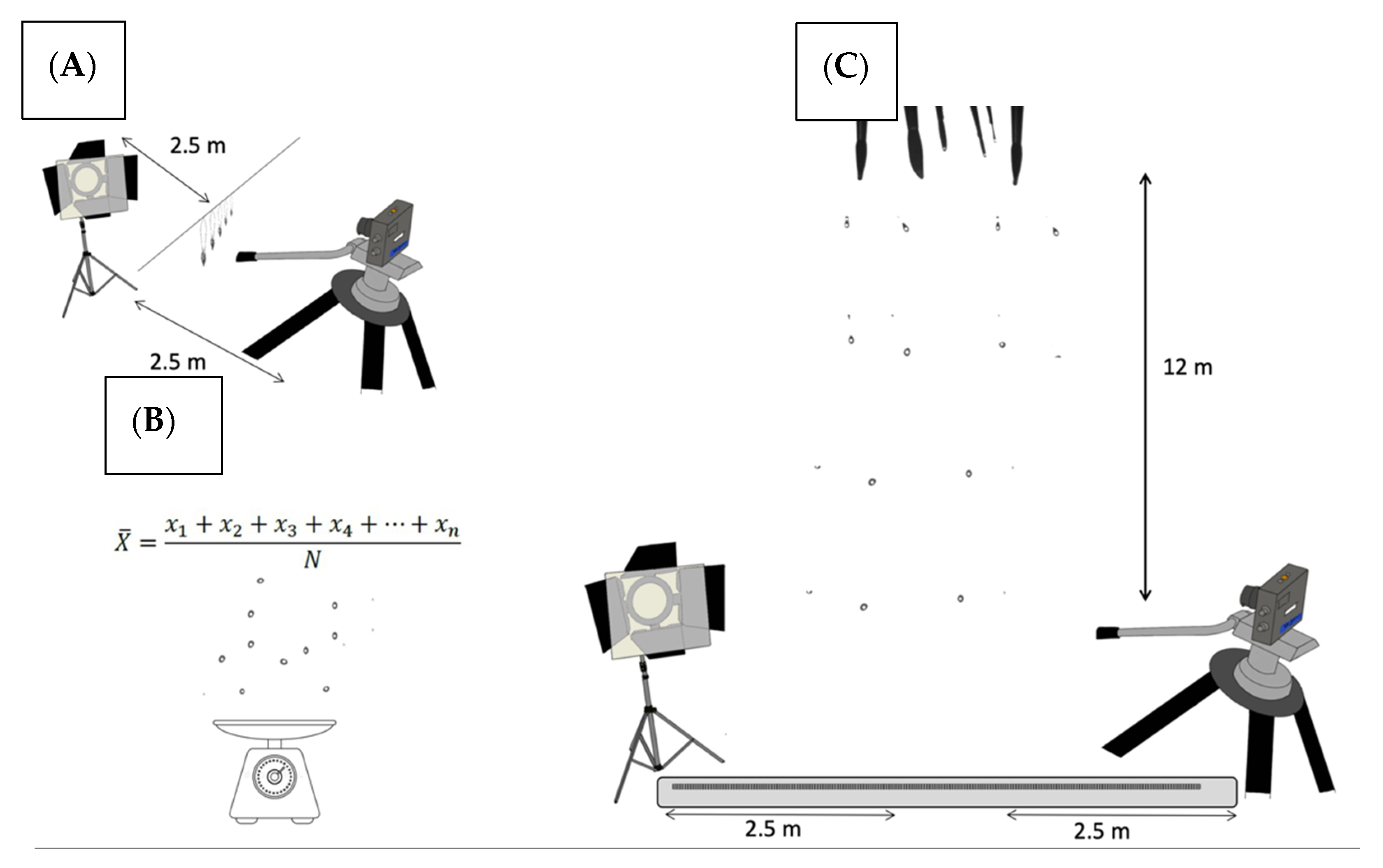
2.2. Experimental Design

2.2.1. First Phase: Calibration and Study of Individual Drops

Work began with the Smart High-Speed Camera. It is important to note that in the videos, the shadows of the drops generated by the light source are the most reflected marks; therefore, the optimal placement of the screen is important to capture these shadows, since they are easier to analyze. The first thing therefore is the calibration of the systems, producing drops of known sizes that fall along the sample area to evaluate if the size that is reflected in the image is adequate. That is why the distance adjustment is very important, and the installation of a ruler at the same distance where the drops are produced allowed for the focusing directly on the drops of the same plane at the same time as it allowed for the comparison of the sizes with a pattern in the form of rule.

To convert from pixels to mm, the ImageJ program was used, and the conversion factor from pixels to mm was obtained to measure the different sizes of the drops. To convert to mm, a known measurement was selected; a cm from the ruler, and that actual size was adjusted to the number of pixels it covered in the photograph. To make this value more accurate, this measurement was performed thirty times with each size, and the average was made.

At first, drops were generated by using several pipettes manually. The camera began to record and in a controlled way individual drops were released. Thus, the first drops could be studied separately, something important when starting with their automatic detection.

Different tests were carried out with the pipette, increasing the number of recorded drops and modifying the drop generation speed, which was performed manually. Tests were also made by increasing the number of frames per second since shape changes were detected in the drops and vibrations in the largest drops (Figure 1).

Subsequently, in order to be able to produce several drops of different sizes at the same time, the drop formation system was modified. Brushes of 5 different sizes began to be used as a means of generating drops with different diameters, to observe how the shape of the drop changed during the fall (Figure 2). The brushes were immersed in water to let them drip, and 10 of those drops per brush were collected on a plate to calculate the average mass of each of the drops produced with the different brushes. Subsequently, once the different sizes had been checked, the brushes were hung on a rope, the brushes were placed in water, and the recording began, with the camera and the light set on both sides to be able to record the drops (Figure 3). Despite the fact that the drops with this method took a long time to precipitate, since they did not fall until there was enough water accumulated on the tip of the brush, it was possible to measure drops of different sizes falling simultaneously.

Once the production of drops of different sizes controlled in a chain had been achieved, it was ensured that said drops could reach the terminal velocity. To perform this, these drops had to be produced at a height of more than 10 m above the camera. For this reason, the brush system was placed at a height of 12 m placing the camera in the lower part (Figure 3). Thus, it was possible to measure the time (in number of frames) a drop took to travel the space of the photo, from which the characteristic terminal velocity of each drop size produced was calculated. Terminal velocity is reached when there is balance between the forces: friction resistance of Stokes, the force of gravity and the forces of thrust.

As the measurements are made on the projected shadow of the generated drops, which have rounded shapes, the figure detection option was selected in the EyeMotion program, and the detection of color changes was used—in this specific case, we detected black (Figure 4). When the program was ready, it proceeded to detect the drops automatically. It was possible to detect during the entire video or by selecting the specific range of frames that one wants to analyze.

The use of the automatic markers generated by the program can cause errors, since the drop to which they are associated disappears from the screen, because it leaves the frame of the photographs in its fall; for example, it automatically searches for another drop, which would imply that the new drop to which it is associated is not recognized as a new individual drop. Therefore, to avoid these problems, this process should always be reviewed manually. In addition, there may be noise in the images, that is, backgrounds that are not perfectly smooth or drops that also suffer horizontal displacement or even insects; therefore, that it is necessary to perform a manual follow-up, adding the markers individually to each drop in each of the frames in which it appears. Otherwise, the marker jumps from the drop to the noisy area and vice versa, such that the resulting measurements are wrong.

Each of the markers used to track was assigned a number, making them unique for each drop, and in this way, it was possible to proceed to represent its acceleration and velocity graph, the data of which are exported to an Excel file, in which we have the data of time, position in the x and y axes, displacement speed and acceleration in these axes.

2.2.2. Second Phase: Calibration of Rain Events Formed by Sets of Drops

Once the parameters of the characteristic sizes and speeds of the drops were known, we were ready to carry out an analysis of several drops at the same time. To carry out this experiment, frames taken in a large rainfall simulator, called “The Wageningen Rainfall Simulator” [55], located in the Netherlands, were used. In it, tests were carried out under various rain intensities, 30, 60, 90 and 125 mm/h. These trials were conducted in 2017 and have not been studied to date. In this case, it is important to distinguish events according to different rainfall intensities, since they involve different numbers of drops. Therefore, the photographs are analyzed by dividing them into 4 different intensities, analyzing the different number of raindrops and their different sizes, and thus being able to make a spectrum of the number of drops per minute for each size.

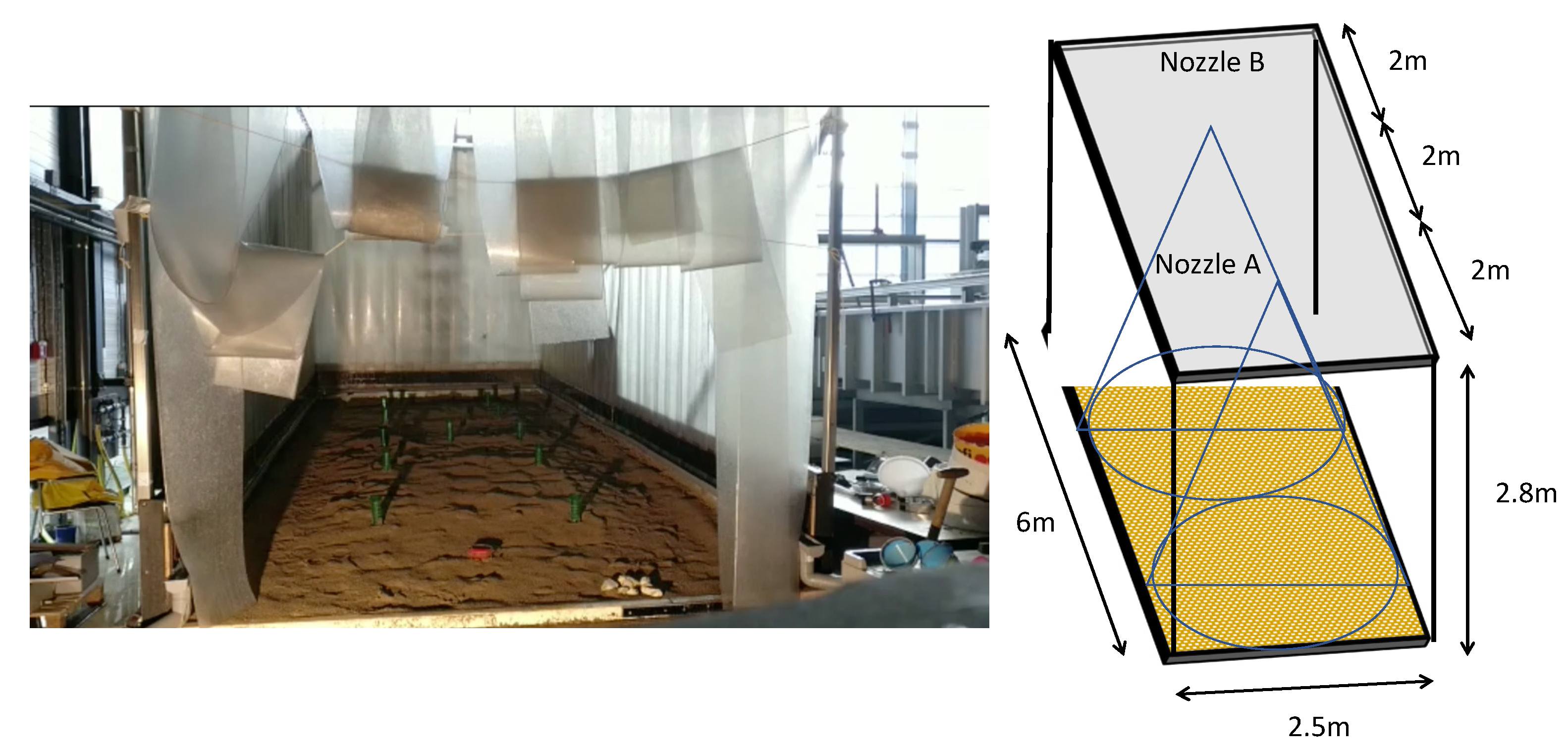
2.2.3. Rainfall Simulator

The rain simulator used is part of the Kraijenhoff van de Leur laboratory for water and sediment dynamics at Wageningen University in the Netherlands. The simulator (Figure 5) is 6 m long and 2.5 m wide, with a height of 2.8 m. The sides of the simulator are covered by a plastic curtain to prevent the surroundings from getting wet. In addition, the simulator plot can be tilted up to 15.5° with a hydraulic lift. There are four nozzles, as described in detail by Lassu [55].

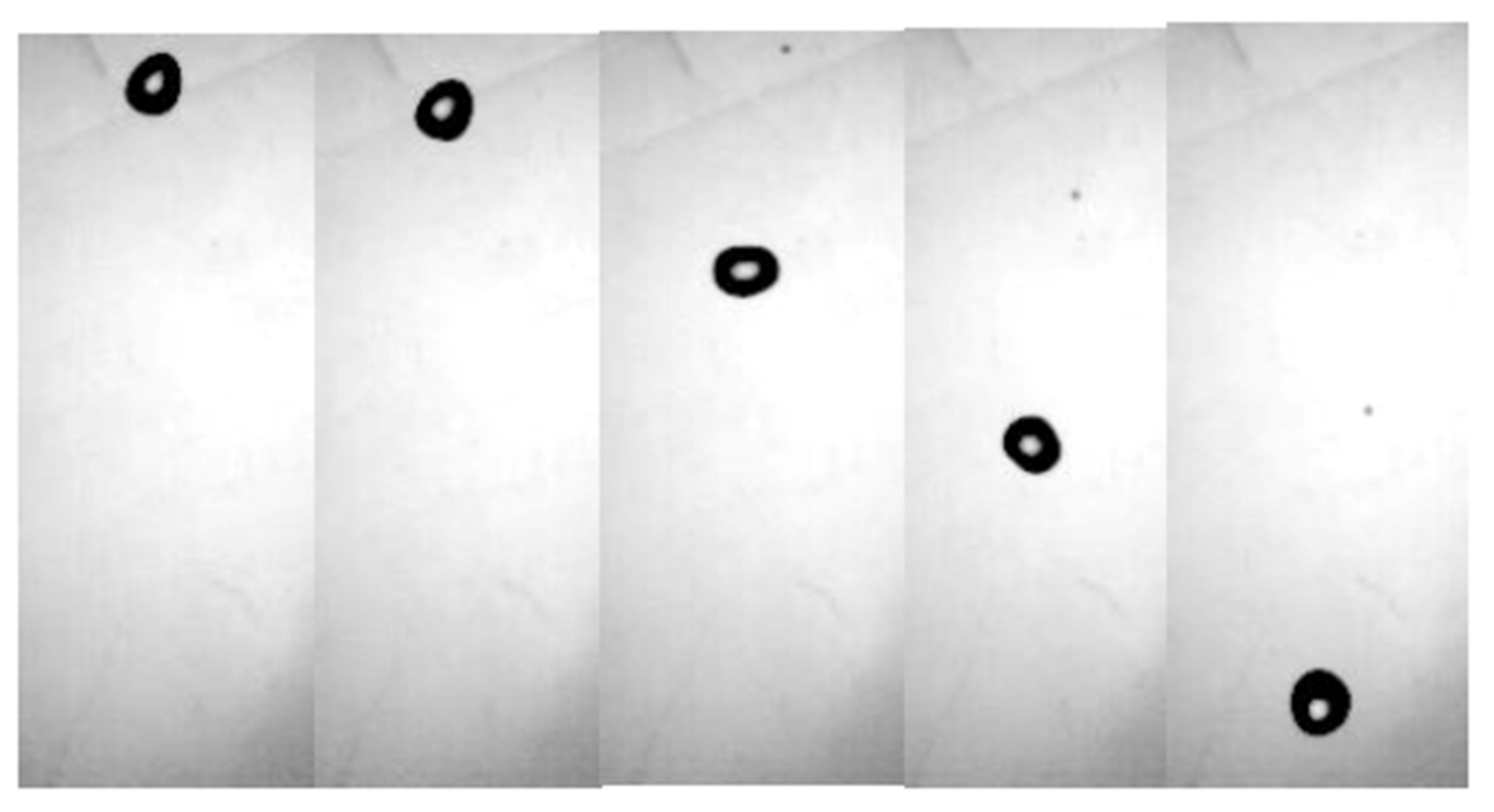
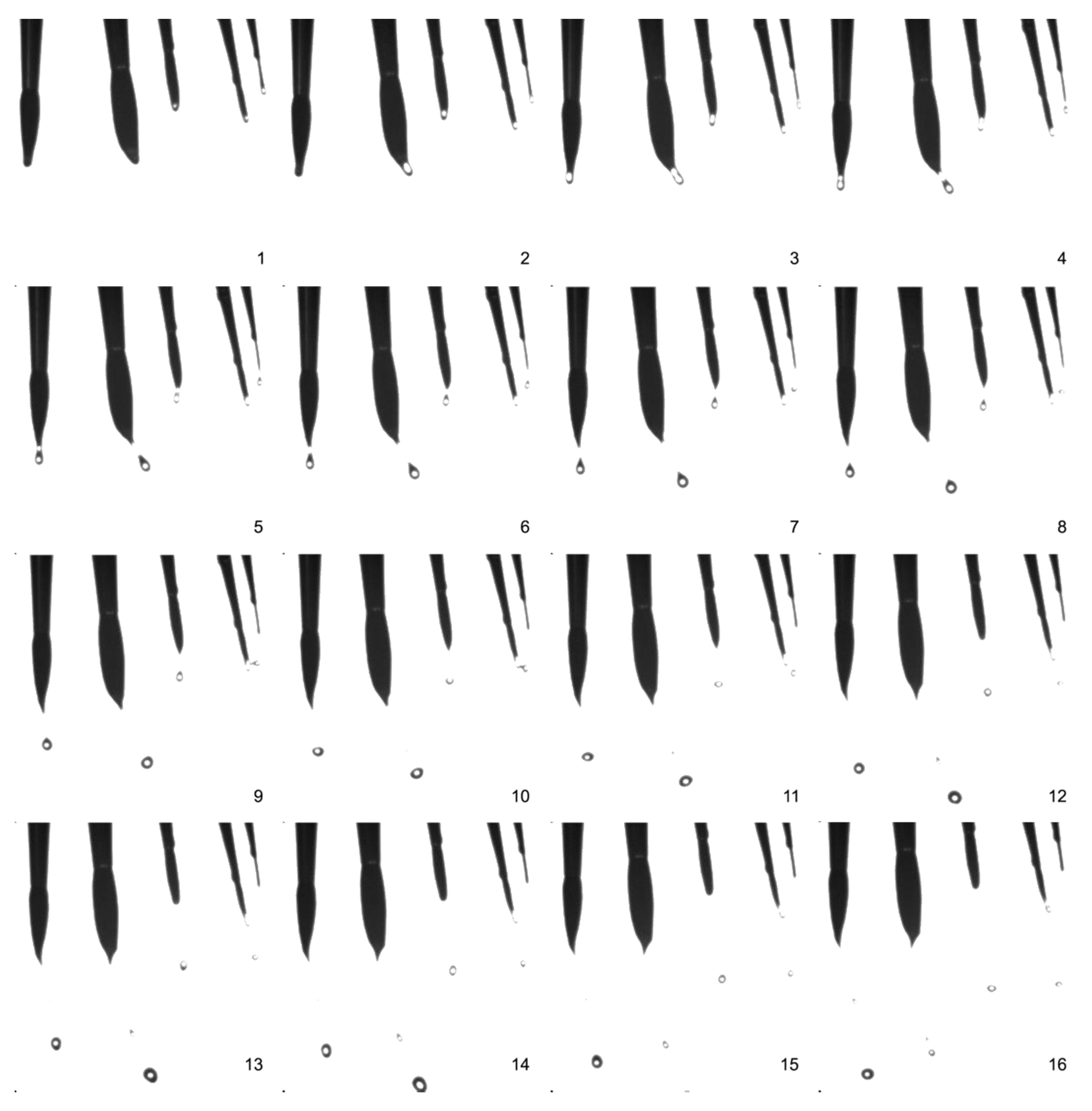
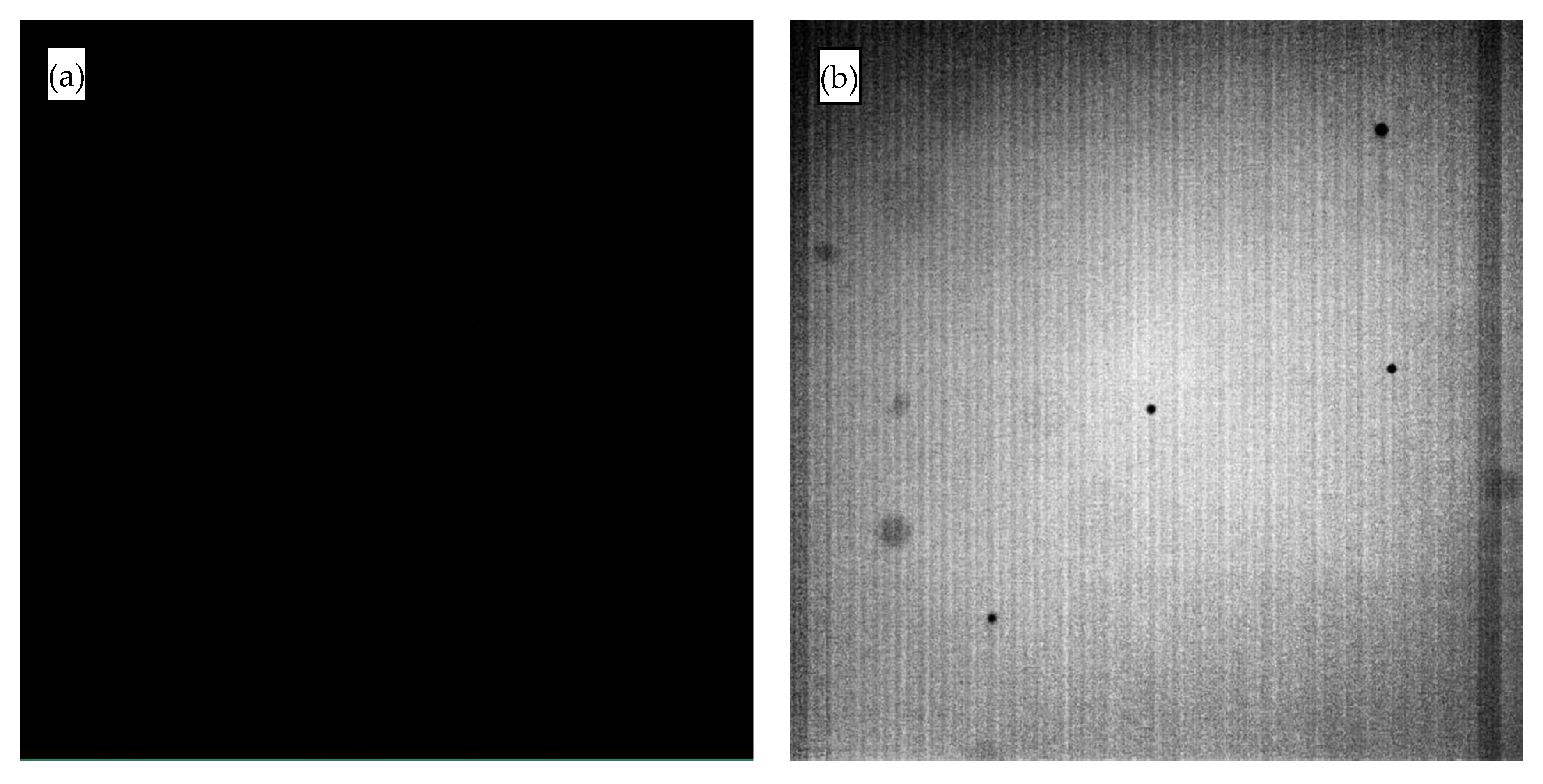
2.2.4. Recording of the Drops

To carry out the experiments, the high-speed camera FASTCAM-APX RS model 250K was used, with which different recordings were made at two points of the rain simulator, below nozzle A and B. Therefore, for each of the rainfall intensities at which the experiment was carried out, there are recordings of the drops at both points, so the results could also be compared between different areas of the simulator.

For each rain intensity, one camera calibration was carried out using, similarly to the first part of the work, a ruler; in this way, it was possible to know the different sizes of the drops, and the definition of the camera could also be adjusted to better distinguish the drops that were at the same distance as the ruler and could thus study them.

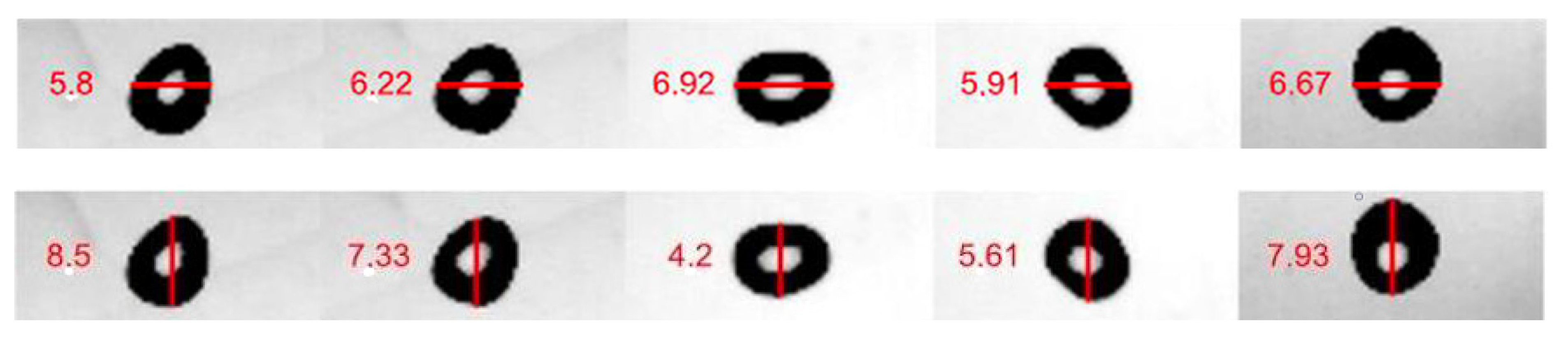
2.2.5. Analysis of Images

An important procedure in this phase of the work was to adjust the contrast of the images, since when compiling them, they were compressed so that they were apparently black, and they required the application of a code that adjusted the contrast with MATLAB (saturates the lower 1% and the top 1% of all pixel values), thereby increasing the contrast of the output image (Figure 6).

The first aspect to take into account was that now they were no longer individual drops, but rather that there were different drops falling at the same time in an area that included different distances from the camera and therefore different depths of field. The selection of the drops and the sample space was based on the sharpness and color of the drops in the image. In this way, an algorithm could be defined that selected only the darkest and most defined drops, which were those that occupy the sample space. The image was scanned with MATLAB, and an Excel file was created with the following variables: the position on the vertical and horizontal axes of the drop, its major and minor axis, and its area. The sizes of the area of the drops in the images were compared with previously chosen sizes, and finally, the number of drops of each size was counted. Although large drops were deformed during their fall and only the smallest retained their spherical shape [20], the measurements of the vertical and horizontal drops allowed for an approximate volume to be assigned to each drop located in the photo. Droplet size ranges were decided upon after considering that in natural rain it is very rare to see drops larger than 5 mm in diameter. Using the studies of other researchers [11,17,56], very large droplets are those that exceed 5.1 mm in diameter. Large drops are those that are between 3.6 and 5.1 mm in diameter; medians are those between 1.7 and 3.6 mm; small are those that are above 0.85 mm; and finally very small are those that did not reach 0.85 mm (

Table 1. Distribution of sizes chosen for the analysis and frames necessary to traverse the sample space.

Drop-Size Classes	Diameter, (x)	Surface (A)	Number of Frames in Frame Traversing
Units	mm	mm2	Frames
Very small	x < 0.85	A < 0.57	16
Small	0.85 < x < 1.7	0.57 < A < 2.27	14
Medium	1.7 < x < 3.6	2.27 < A < 10.18	11
Big	3.6 < x < 5.1	10.18 < A < 20.43	9
Very big	5.1 < x	20.43< A	8

). Furthermore, it was necessary to make a selection of frames to count the number of drops, since the same drop appeared in different positions in different numbers of photos, depending on its terminal velocity. For this reason, a specific study was conducted on the number of frames that each drop travels according to its size (Table 1).

3. Results and Discussion

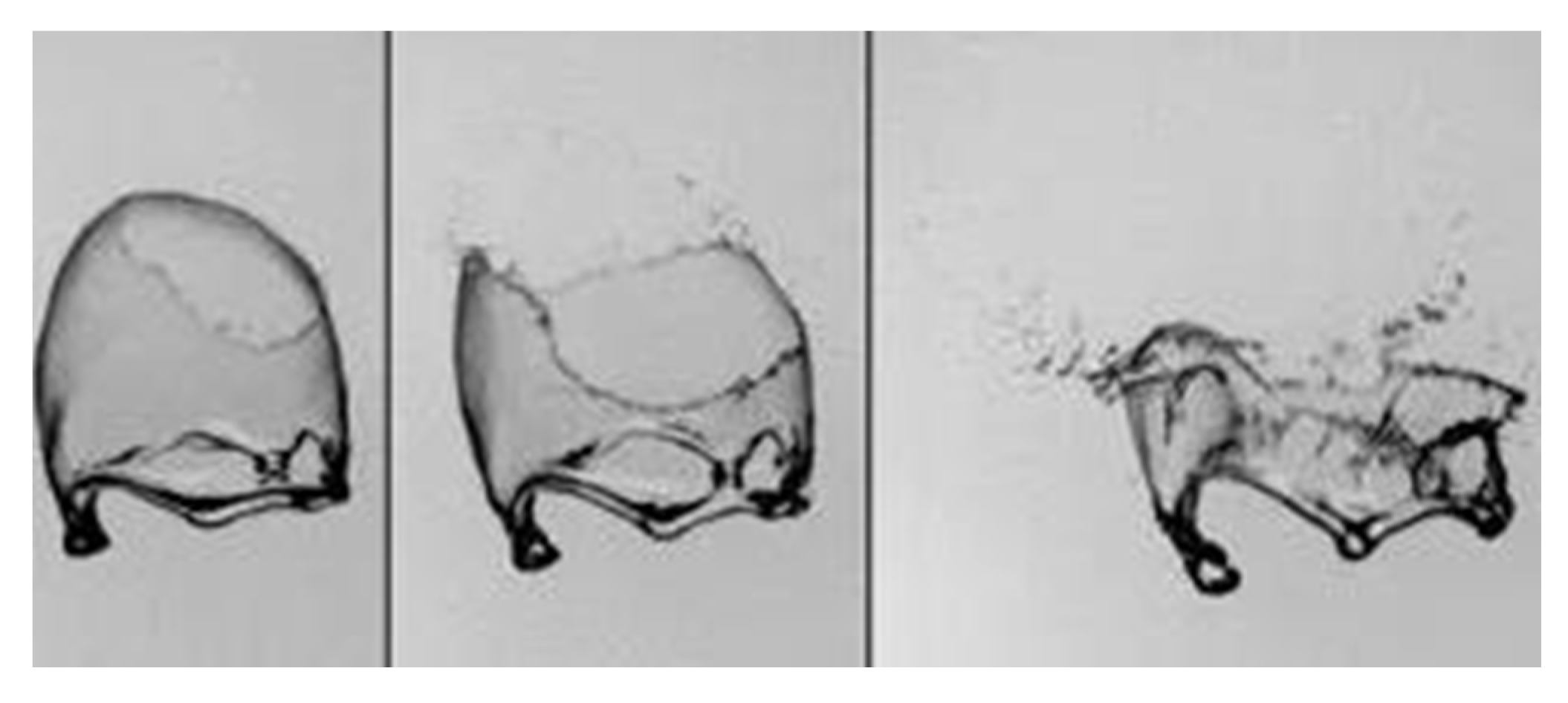
3.1. Measuring Accelerating Drops

With the markers correctly added to the drops, a table was obtained with the necessary values to make an analysis of the position, velocity, acceleration and trajectory of the drops. The most relevant for the study being carried out are time, position on the y-axis, velocity on that axis and acceleration. In the first moments, the speed increases until it reaches a more stable value, corresponding to its terminal velocity, while the acceleration remains stable.

Speed increases as time passes, and because the photographs were taken of drops which did not have enough distance to reach their terminal speeds, these drops were still in its acceleration phase. The last variable is acceleration, d²y/dt², which is expressed in pixels per millisecond squared. It is difficult to know the exact acceleration of the drops using this method as there can be small margins of error due to precision errors when using the markers.

Another relevant observation of this experiment was the study of the deformation of the drops during their fall. During their acceleration phase, the drops present deformations while they fall, which is due to the force exerted by the air on the drop and the force exerted by the particles of the drop to stay together. If the drops were too large, it would end up breaking (Figure 7) because of the air.

As a general rule, drops larger than 5 mm in diameter are very difficult to see in nature. This phenomenon can also be seen in the tests carried out with the brushes. The deformation of the drops can be seen in the Figure 1: the drop during its fall does not maintain the same shape but undergoes oscillations and breaks into several drops when it exceeds 5 mm. If drops are released from a height greater than 10 m, they can be produced in large sizes, and if the intention is to launch them from lower heights by gravity, it is recommended that the drops are generated using very fine brushes (less than 1 mm) so that drops are available of different sizes but similar in size to natural rain, since the drops generated are always greater than the size of the tips of the brushes.

3.2. Terminal Velocity

For drops falling at terminal velocity, the velocities of the drops were analyzed according to their size resulting in three different speeds for the three sizes of drops that were generated: 2, 3 and 4 mm. The drops generated by the 2 mm tube all had similar speeds of 15–16 px/ms (4.90 and 5.22 m/s); the 3 mm drops had a speed between 18 and 19 px/ms (between 5.88 and 6.20 m/s); and those of 4 mm, registered speeds between 21 and 22 px/ms (6.87 and 7.18 m/s). In this experiment, it was also possible to see the behavior of the drops with respect to their shape, and it was observed that the largest drops flattened, acquiring an “ovaloid” shape (the drop is not round but seems to be flattened at its upper and lower ends).

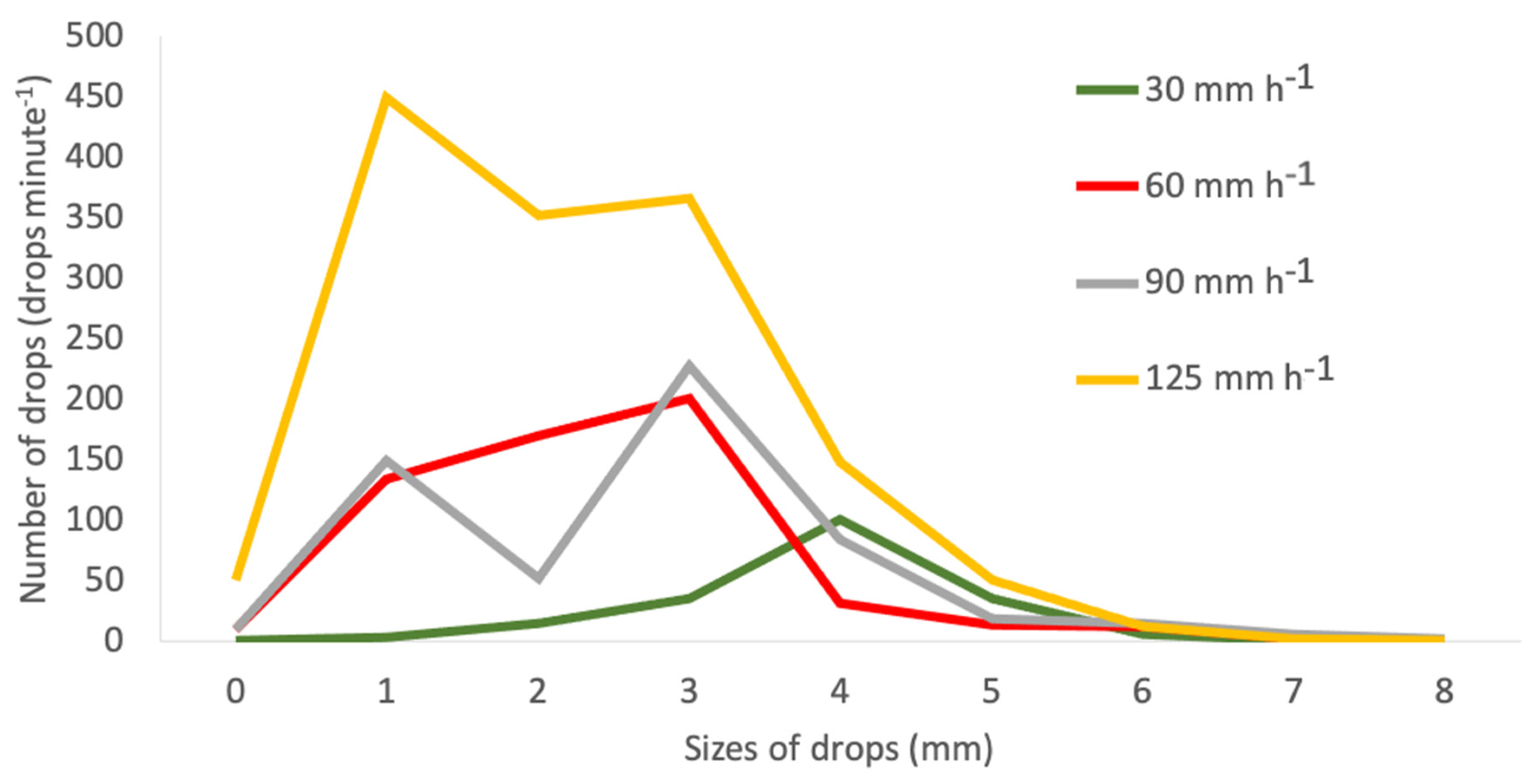
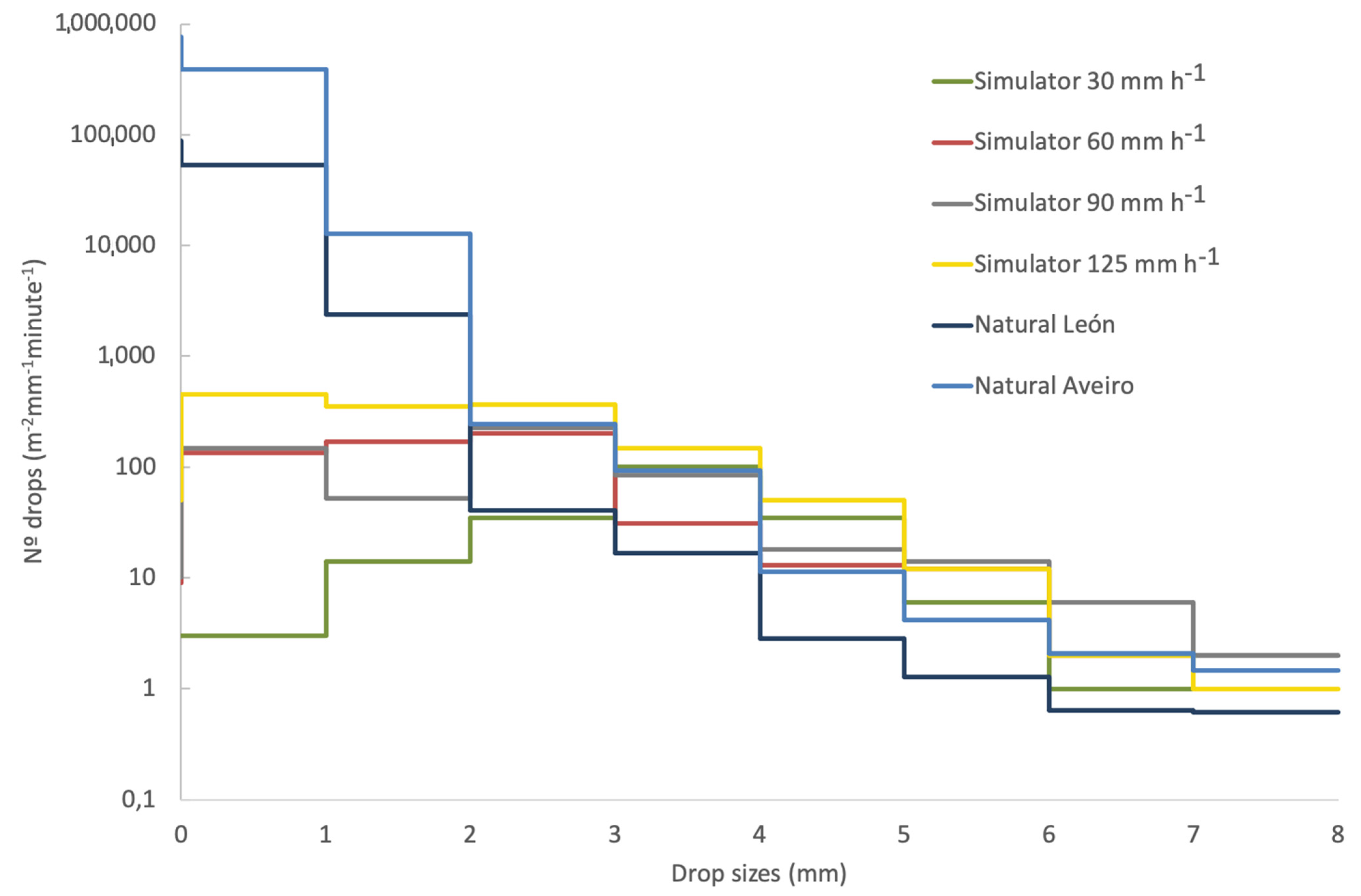
3.3. Calibration of Simulator Based on the Analysis of Pictures

In the first place, an attempt was made to make a measurement of the intensity of rain through the coefficient of uniformity of Christiansen [58], which has indicated that there is a precipitation uniformity of 71–82%. However, this method only indicates the amount of water collected per time, without specifying the sizes of raindrops or their velocities. That is why we are going to complement the calibration by studying with a high-speed camera, taking photos both under nozzle A and under nozzle B (Figure 5). Subsequently, an integration of the data was carried out in both nozzles, in order to conclude the distribution of droplet sizes throughout the entire area of the rain simulator. In addition, we repeated this study with four intensities (30, 60, 90 and 125 mm/h).

From the analysis of the drop-size distributions taken with both nozzles with the different intensities, it was observed that in all cases nozzle A presents a greater number of drops. Furthermore, an increase in the intensity of rain supposes a direct increase in the number of registered drops. Likewise, it can be observed that with an intensity of 30 mm/h, in nozzle A, a higher number of medium and large drops was detected than in the rest of the sizes, the majority concentrating around 4 mm in diameter (Figure 8). The integration of the two nozzles shows that the mean drop-size value is lower when the intensity of the rainfall simulator increases (Figure 9)

The number of drops registered by nozzle B is considerably less than in nozzle A, which is due to the fact that nozzle B is located in a position closer to the pump; therefore, there is less probability of blockages in the network due to impurities and also a lower pressure loss.

With an intensity of 60 mm/h, we have a considerable increase in the number of small drops in camera A, especially in drops with diameters of 1 mm, although there are still more medium drops (Figure 5). In the case of nozzle B, a general decrease in the number of drops is once again seen, especially the small ones. Once the data from nozzle A and B with the intensity of 60 mm/h are added, it can be seen that in this case there are far more drops than in the measurements with intensity of 30 mm/h, with a quite considerable increase in the drops of 1 mm in diameter.

With an intensity of 90 mm/h, there are many more drops of 1 mm diameter in nozzle A compared to the previous measurements, while in nozzle B, the number of medium drops is still much higher. When added together, two peaks are clearly visible: one at 1 mm and the other at 4 mm. In the recordings of nozzle A in the 125 mm/h experiment, a clear increase in the number of drops of all sizes is seen, considerably noticeable in the medium and small ones. The picture with nozzle B recorded a very different drop distribution compared to the rest of the intensities, with the number of small drops being very high and the spectrum of the number of drops per size completely changing. In the sum of the number of drops registered by each one of the nozzles in the rain intensity of 125 mm/h, it is seen how the number of drops is much greater than in the rest of intensities, especially the small drops of 1 mm, which undergo very large growth.

In the graphs, we can see how as the intensity of rain increases, there is a greater number of drops per minute, especially drops with sizes close to 1 mm in diameter. This may be because in the simulator, the drops are produced with a pump and increasing the pressure to produce greater intensity produces smaller drops.

It is very striking to observe the great difference in the drop-size distribution (DSD) of the simulated rainfall with the natural rain spectra obtained by Fernández-Raga [59] (Figure 10), which would adopt an exponential or gamma form [47,56,60]. Sizes smaller than 1 mm in diameter show a higher number of drops in the natural rainfall, but with drops bigger than 2 mm in diameter, the number of drops is much more comparable. This means that the simulator can be used to evaluate the erodibility of soils, despite the fact that in erosion processes, not all droplet sizes are equally important, since droplet sizes less than 1 mm hardly have an impact [11,17], as they are able to pull up very few aggregates from the natural terrain due to the fact that their terminal velocity is also related to their size, resulting in a very small kinetic energy [61]. This kinetic energy is truly responsible for the splashed particles (which is the total energy transferred to the particles in order to eject and displace them). In any case, the form of the DSD is very different under natural or simulated rainfall, and consequently, the kinetic energy associated to the natural or simulated events is also different. According to the available literature, the energy values of the ejected particles in relation to the falling drops are between 0.2% and 45%, which was demonstrated by diverse authors using various techniques and experimental conditions. However, it should be noted that previous research in this field has been based primarily on experiments in which the splashed material was treated only as water droplets when the impacting drop hit the surface of a liquid of different thicknesses [62,63,64] or solid-phase particles, mostly grains of sand [34].

4. Conclusions

A study was conducted on how the drops of water deform during their fall, in which it was seen that the drops do not have the same shape during the entire fall path and that only the smaller drops, when they have sufficient speed, present a round shape, while the larger ones are flattened and have an “ovaloid” shape. It was possible to successfully carry out an experiment in which the terminal velocity of water drops with different sizes, previously established, falling from more than 6 m in height was measured, finding that the drops in free fall of 2 mm in diameter have a speed of 5 m/s, drops of 3 mm have a speed of 6 m/s, and drops of 4 mm have a speed of 7 m/s.

Regarding the second phase, rain images were used made in a rain simulator in the Netherlands, and it was observed that, with a greater intensity of rain, there were more drops, and the peak of the graph moved toward the area where the drops were minor. This is due to the fact that because it is simulated rain, increasing the intensity leads to a higher nozzle pressure; therefore, the drops that are produced are smaller, which contrasts with real rain, in which just the opposite happens. This is why it is necessary to calibrate the rain simulators, to be able to evaluate their resemblance to reality, calculate the real kinetic energy of the rain they produce, and see if they can be used to model events in nature.

In addition, several aspects must be taken into account when selecting the drops at the indicated distance to be able to study them, with a controlled space to be able to give the values per unit area in the images since the camera records drops that pass too close or too far from the camera’s calibration point, making these droplets appear larger and smaller than they actually are. This was solved by eliminating those droplets that appear out of focus on the camera. On the other hand, the use of the camera is more comfortable and cheaper when performing this type of study, and results that are in line with reality are achieved.

References

1. Chang, W.-Y.; Lee, G.; Jou, B.J.-D.; Lee, W.-C.; Lin, P.-L.; Yu, C.-K. Uncertainty in Measured Raindrop Size Distributions from Four Types of Collocated Instruments. Remote Sens. 2020, 12, 1167. [Google Scholar] [CrossRef] [Green Version]
2. Altaratz, O.; Koren, I.; Reisin, T.; Kostinski, A.; Feingold, G.; Levin, Z.; Yin, Y. Aerosols’ Influence on the Interplay between Condensation, Evaporation and Rain in Warm Cumulus Cloud. Atmos. Chem. Phys. 2008, 8, 15–24. [Google Scholar] [CrossRef] [Green Version]
3. Yu, S. Water Spray Geoengineering to Clean Air Pollution for Mitigating Haze in China’s Cities. Environ. Chem. Lett. 2014, 12, 109–116. [Google Scholar] [CrossRef]
4. Han, C.; Feng, L.; Huo, J.; Deng, Z.; Zhang, G.; Ji, B.; Zhou, Y.; Bi, Y.; Duan, S.; Yuan, R. Characteristics of Rain-Induced Attenuation over Signal Links at Frequency Ranges of 25 and 38 GHz Observed in Beijing. Remote Sens. 2021, 13, 2156. [Google Scholar] [CrossRef]
5. Şeker, Ş.; Kunter, F. Simulation of Discrete Electromagnetic Propagation Model for Atmospheric Effects on Mobile Communication. Turk. J. Electr. Eng. Comput. Sci. 2013, 21, 1944–1955. [Google Scholar] [CrossRef]
6. Lam, H.Y.; Luini, L.; Din, J.; Alhilali, M.J.; Jong, S.L.; Cuervo, F. Impact of Rain Attenuation on 5G Millimeter Wave Communication Systems in Equatorial Malaysia Investigated through Disdrometer Data. In Proceedings of the 2017 11th European Conference on Antennas and Propagation (EUCAP), Paris, France, 19–24 March 2017; pp. 1793–1797. [Google Scholar]
7. Blanco-Alegre, C.; Castro, A.; Calvo, A.I.; Oduber, F.; Fernández-González, D.; Valencia-Barrera, R.M.; Vega-Maray, A.M.; Molnár, T.; Fraile, R. Towards a Model of Wet Deposition of Bioaerosols: The Raindrop Size Role. Sci. Total Environ. 2021, 767, 145426. [Google Scholar] [CrossRef] [PubMed]
8. Pérez-Rodríguez, P.; Paradelo, M.; Rodríguez-Salgado, I.; Fernández-Calviño, D.; López-Periago, J.E. Modeling the Influence of Raindrop Size on the Wash-off Losses of Copper-Based Fungicides Sprayed on Potato (Solanum tuberosum L.) Leaves. J. Environ. Sci. Health Part B 2013, 48, 737–746. [Google Scholar] [CrossRef]
9. Pérez-Rodríguez, P.; Paradelo, M.; Soto-Gómez, D.; Fernández-Calviño, D.; López-Periago, J.E. Modeling Losses of Copper-Based Fungicide Foliar Sprays in Wash-off under Simulated Rain. Int. J. Environ. Sci. Technol. 2015, 12, 661–672. [Google Scholar] [CrossRef] [Green Version]
10. Beczek, M.; Ryżak, M.; Sochan, A.; Mazur, R.; Polakowski, C.; Bieganowski, A. A New Approach to Kinetic Energy Calculation of Two-Phase Soil Splashed Material. Geoderma 2021, 396, 115087. [Google Scholar] [CrossRef]
11. Fernández-Raga, M.; Gutiérrez, E.G.; Keesstra, S.D.; Tárrega, R.; Nunes, J.P.; Marcos, E.; Rodrigo-Comino, J. Determining the Potential Impacts of Fire and Different Land Uses on Splash Erosion in the Margins of Drylands. J. Arid Environ. 2021, 186, 104419. [Google Scholar] [CrossRef]
12. Fernández-Raga, M.; García-Díez, I.; Campo, J.; Viejo, J.; Palencia, C. Effectiveness of a New Drainage System for Decreasing Erosion in Road Hillslopes. Air Soil Water Res. 2021, 14, 1178622120988722. [Google Scholar] [CrossRef]
13. Fernández-Raga, M.; Palencia, C.; Keesstra, S.; Jordán, A.; Fraile, R.; Angulo-Martínez, M.; Cerdà, A. Splash Erosion: A Review with Unanswered Questions. Earth-Sci. Rev. 2017, 171, 463–477. [Google Scholar] [CrossRef] [Green Version]
14. Kinnell, P.I.A. Raindrop-Impact-Induced Erosion Processes and Prediction: A Review. Hydrol. Process. 2005, 19, 2815–2844. [Google Scholar] [CrossRef]
15. Morgan, R.P.C. Field Studies of Rainsplash Erosion. Earth Surf. Process. 1978, 3, 295–299. [Google Scholar] [CrossRef]
16. Van Dijk, A.I.J.M.; Bruijnzeel, L.A.; Rosewell, C.J. Rainfall Intensity–Kinetic Energy Relationships: A Critical Literature Appraisal. J. Hydrol. 2002, 261, 1–23. [Google Scholar] [CrossRef]
17. Fernández-Raga, M.; Campo, J.; Rodrigo-Comino, J.; Keesstra, S.D. Comparative Analysis of Splash Erosion Devices for Rainfall Simulation Experiments: A Laboratory Study. Water 2019, 11, 1228. [Google Scholar] [CrossRef] [Green Version]
18. Grigar, J.; Duiker, S.W.; Flanagan, D.C. Understanding Soil Erosion by Water to Improve Soil Conservation. Crop. Soils 2020, 53, 47–55. [Google Scholar] [CrossRef]
19. Nie, X.; Li, Z.; Huang, J.; Liu, L.; Xiao, H.; Liu, C.; Zeng, G. Thermal Stability of Organic Carbon in Soil Aggregates as Affected by Soil Erosion and Deposition. Soil Tillage Res. 2018, 175, 82–90. [Google Scholar] [CrossRef]
20. Fernández-Raga, M.; Fraile, R.; Keizer, J.J.; Varela Teijeiro, M.E.; Castro, A.; Palencia, C.; Calvo, A.I.; Koenders, J.; Da Costa Marques, R.L. The Kinetic Energy of Rain Measured with an Optical Disdrometer: An Application to Splash Erosion. Atmos. Res. 2010, 96, 225–240. [Google Scholar] [CrossRef]
21. Fu, Y.; Li, G.; Zheng, T.; Zhao, Y.; Yang, M. Fragmentation of Soil Aggregates Induced by Secondary Raindrop Splash Erosion. CATENA 2020, 185, 104342. [Google Scholar] [CrossRef]
22. An, J.; Zheng, F.L.; Han, Y. Effects of Rainstorm Patterns on Runoff and Sediment Yield Processes. Soil Sci. 2014, 179, 293–303. [Google Scholar] [CrossRef]
23. Helming, K.; Auzet, A.-V.; Favis-Mortlock, D. Soil Erosion Patterns: Evolution, Spatio-Temporal Dynamics and Connectivity. Earth Surf. Process. Landf. 2005, 30, 131–132. [Google Scholar] [CrossRef]
24. Nearing, M.A. Why Soil Erosion Models Over-Predict Small Soil Losses and under-Predict Large Soil Losses. Catena 1998, 32, 15–22. [Google Scholar] [CrossRef]
25. Savat, J. Work Done by Splash: Laboratory Experiments. Earth Surf. Process. Landf. 1981, 6, 275–283. [Google Scholar] [CrossRef]
26. Wainwright, J.; Parsons, A.J.; Cooper, J.R.; Gao, P.; Gillies, J.A.; Mao, L.; Orford, J.D.; Knight, P.G. The Concept of Transport Capacity in Geomorphology. Rev. Geophys. 2015, 53, 1155–1202. [Google Scholar] [CrossRef]
27. Kukal, S.; Sarkar, M. Laboratory Simulation Studies on Splash Erosion and Crusting in Relation to Surface Roughness and Raindrop Size. J. Indian Soc. Soil Sci. 2011, 59, 87–93. [Google Scholar]
28. Zumr, D.; Mützenberg, D.V.; Neumann, M.; Jeřábek, J.; Laburda, T.; Kavka, P.; Johannsen, L.L.; Zambon, N.; Klik, A.; Strauss, P.; et al. Experimental Setup for Splash Erosion Monitoring—Study of Silty Loam Splash Characteristics. Sustainability 2020, 12, 157. [Google Scholar] [CrossRef] [Green Version]
29. Almeida, Á.M.R.; Sibaldelli, R.N.R.; de Oliveira Negrão Lopes, I.; de Oliveira, M.C.N.; Farias, J.R.B. Horizontal and Vertical Droplet Dispersion Mimicking Soybean—Septoria Glycines Pathosystem. Eur. J. Plant Pathol. 2019, 154, 437–443. [Google Scholar] [CrossRef]
30. Lee, D.; Tertuliano, M.; Harris, C.; Vellidis, G.; Levy, K.; Coolong, T. Salmonella Survival in Soil and Transfer Onto Produce via Splash Events. J. Food Prot. 2019, 82, 2023–2037. [Google Scholar] [CrossRef]
31. Ao, C.; Yang, P.; Zeng, W.; Jiang, Y.; Chen, H.; Xing, W.; Zha, Y.; Wu, J.; Huang, J. Development of an Ammonia Nitrogen Transport Model from Surface Soil to Runoff via Raindrop Splashing. CATENA 2020, 189, 104473. [Google Scholar] [CrossRef]
32. Hu, F.; Liu, J.; Xu, C.; Wang, Z.; Liu, G.; Li, H.; Zhao, S. Soil Internal Forces Initiate Aggregate Breakdown and Splash Erosion. Geoderma 2018, 320, 43–51. [Google Scholar] [CrossRef]
33. Beczek, M.; Ryzak, M.; Sochan, A.; Mazur, R.; Bieganowski, A. The Mass Ratio of Splashed Particles during Raindrop Splash Phenomenon on Soil Surface. Geoderma 2019, 347, 40–48. [Google Scholar] [CrossRef]
34. Long, E.J.; Hargrave, G.K.; Cooper, J.R.; Kitchener, B.G.B.; Parsons, A.J.; Hewett, C.J.M.; Wainwright, J. Experimental Investigation into the Impact of a Liquid Droplet onto a Granular Bed Using Three-Dimensional, Time-Resolved, Particle Tracking. Phys. Rev. E 2014, 89, 0322010. [Google Scholar] [CrossRef] [Green Version]
35. Marzen, M.; Iserloh, T.; de Lima, J.L.M.P.; Ries, J.B. The Effect of Rain, Wind-Driven Rain and Wind on Particle Transport under Controlled Laboratory Conditions. Catena 2016, 145, 47–55. [Google Scholar] [CrossRef]
36. Sochan, A.; Łagodowski, Z.A.; Nieznaj, E.; Beczek, M.; Ryzak, M.; Mazur, R.; Bobrowski, A.; Bieganowski, A. Splash of Solid Particles as a Stochastic Point Process. J. Geophys. Res. Earth Surf. 2019, 124, 2475–2490. [Google Scholar] [CrossRef]
37. Kathiravelu, G.; Lucke, T.; Nichols, P. Rain Drop Measurement Techniques: A Review. Water 2016, 8, 29. [Google Scholar] [CrossRef] [Green Version]
38. Xiao, H.; Liu, G.; Abd-Elbasit, M.A.M.; Zhang, X.C.; Liu, P.L.; Zheng, F.L.; Zhang, J.Q.; Hu, F.N. Effects of Slaking and Mechanical Breakdown on Disaggregation and Splash Erosion. Eur. J. Soil Sci. 2017, 68, 797–805. [Google Scholar] [CrossRef]
39. Vaezi, A.R.; Ahmadi, M.; Cerdà, A. Contribution of Raindrop Impact to the Change of Soil Physical Properties and Water Erosion under Semi-Arid Rainfalls. Sci. Total Environ. 2017, 583, 382–392. [Google Scholar] [CrossRef]
40. Xiao, H.; Liu, G.; Zhang, Q.; Fenli, Z.; Zhang, X.; Liu, P.; Zhang, J.; Hu, F.; Elbasit, M.A.M.A. Quantifying Contributions of Slaking and Mechanical Breakdown of Soil Aggregates to Splash Erosion for Different Soils from the Loess Plateau of China. Soil Tillage Res. 2018, 178, 150–158. [Google Scholar] [CrossRef]
41. Kinnell, P.I.A. The Influence of Time and Other Factors on Soil Loss Produced by Rain-Impacted Flow under Artificial Rainfall. J. Hydrol. 2020, 587, 125004. [Google Scholar] [CrossRef]
42. Fu, Y.; Li, G.; Zheng, T.; Li, B.; Zhang, T. Splash Detachment and Transport of Loess Aggregate Fragments by Raindrop Action. CATENA 2017, 150, 154–160. [Google Scholar] [CrossRef]
43. Li, G.; Fu, Y.; Li, B.; Zheng, T.; Wu, F.; Peng, G.; Xiao, T. Micro-Characteristics of Soil Aggregate Breakdown under Raindrop Action. CATENA 2018, 162, 354–359. [Google Scholar] [CrossRef]
44. Hudson, N. Raindrop Characteristics in South Central United States. Rhod. J. Agric. Res. 1963, 1, 6–11. [Google Scholar]
45. Hall, M.J. Use of Stain Method in Determining the Drop-Size Distributions of Coarse Liquid Sprays. Trans. ASAE 1970, 13, 33–41. [Google Scholar] [CrossRef]
46. Pruppacher, H.R.; Beard, K.V. A wind tunnel investigation of the internal circulation and shape of water drops falling at terminal velocity in air. Q. J. R. Meteorol. Soc. 1970, 96, 247–256. [Google Scholar] [CrossRef]
47. Angulo-Martínez, M.; Beguería, S.; Latorre, B.; Fernández-Raga, M. Comparison of Precipitation Measurements by OTT Parsivel2 and Thies LPM Optical Disdrometers. Hydrol. Earth Syst. Sci. 2018, 22, 2811–2837. [Google Scholar] [CrossRef] [Green Version]
48. Johannsen, L.L.; Zambon, N.; Strauss, P.; Dostal, T.; Neumann, M.; Zumr, D.; Cochrane, T.A.; Blöschl, G.; Klik, A. Comparison of Three Types of Laser Optical Disdrometers under Natural Rainfall Conditions. Hydrol. Sci. J. 2020, 65, 524–535. [Google Scholar] [CrossRef]
49. Bartholomew, M.J. Impact Disdrometers Instrument Handbook; DOE/SC-ARM-TR—111; Department of Energy, Office of Science, Office of Biological and Environmental Research: Brookhaven, NY, USA, 2016; p. 1251384. [Google Scholar]
50. Tokay, A.; Kruger, A.; Krajewski, W. Comparison of Drop Size Distribution Measurements by Impact and Optical Disdrometers. J. Appl. Meteorol. 2001, 40, 2083–2097. [Google Scholar] [CrossRef]
51. Testik, F.Y.; Rahman, M.K. High-Speed Optical Disdrometer for Rainfall Microphysical Observations. J. Atmos. Ocean. Technol. 2016, 33, 231–243. [Google Scholar] [CrossRef]
52. Gunn, R.; Kinzer, G.R. Terminal Velocity of Water Droplets in Stagnant Air. J. Meteorol. 1949, 6, 243–248. [Google Scholar] [CrossRef] [Green Version]
53. Marshall, J.S.; Palmer, W.M. Relation of Drop Size to Intensity. J. Meteorol. 1948, 5, 165–166. [Google Scholar] [CrossRef]
54. Schneider, C.A.; Rasband, W.S.; Eliceiri, K.W. NIH Image to ImageJ: 25 Years of Image Analysis. Nat Methods 2012, 9, 671–675. [Google Scholar] [CrossRef]
55. Lassu, T.; Seeger, M.; Peters, P.; Keesstra, S.D. The Wageningen Rainfall Simulator: Set-up and Calibration of an Indoor Nozzle-Type Rainfall Simulator for Soil Erosion Studies. Land Degrad. Dev. 2015, 26, 604–612. [Google Scholar] [CrossRef]
56. Seela, B.K.; Janapati, J.; Lin, P.-L.; Wang, P.K.; Lee, M.-T. Raindrop Size Distribution Characteristics of Summer and Winter Season Rainfall Over North Taiwan. J. Geophys. Res. Atmos. 2018, 123, 11,602–611,624. [Google Scholar] [CrossRef] [Green Version]
57. De la Goutte D’eau à la Pluie—Sciences et Avenir. Available online: https://www.sciencesetavenir.fr/fondamental/de-la-goutte-d-eau-a-la-pluie_22425 (accessed on 14 September 2021).
58. Christiansen, J.E. Irrigation by Sprinkling; Agricultural Experiment Station, University of California: Berkeley, CA, USA; p. 1942.
59. Fernández-Raga, M.; Fraile, R.; Palencia, C.; Marcos, E.; Castañón, A.M.; Castro, A. The Role of Weather Types in Assessing the Rainfall Key Factors for Erosion in Two Different Climatic Regions. Atmosphere 2020, 11, 443. [Google Scholar] [CrossRef]
60. Fernández-Raga, M.; Castro, A.; Palencia, C.; Calvo, A.; Fraile, R. Rain Events on 22 October 2006 in León (Spain): Drop Size Spectra. Atmos. Res. Atmos. Res. 2009, 93, 619–635. [Google Scholar] [CrossRef]
61. Roldán Soriano, M.; Fernandez Yuste, J.A. Sociedad Española de Ciencias Forestales. 2011, pp. 89–95. Available online: https://dialnet.unirioja.es/servlet/articulo?codigo=4244319 (accessed on 16 September 2021).
62. Mutchler, C.K.; Larson, C.L. Splash Amounts from Waterdrop Impact on a Smooth Surface. Water Resour. Res. 1971, 7, 195–200. [Google Scholar] [CrossRef]
63. Ferreira, A.G.; Singer, M.J. Energy Dissipation for Water Drop Impact into Shallow Pools1. Soil Sci. Soc. Am. J. 1985, 49, 1537. [Google Scholar] [CrossRef]
64. Planchon, O.; Mouche, E. A Physical Model for the Action of Raindrop Erosion on Soil Microtopography. Soil Sci. Soc. Am. J. 2010, 74, 1092. [Google Scholar] [CrossRef]
Figure 1. Shape changes detected in falling the drops in pixels.
Water 13 02851 g001aWater 13 02851 g001b
Figure 2. Brushes of 5 different sizes used as a means of generating drops with different diameters in 16 repetitions.
Water 13 02851 g002
Figure 3. Outline of the stages followed in the development and calibration of the methodology. (A): Setup of camera and light to take images of the 5 different brushes (Figure 2). (B): Deriving the mean weight of a drop for a specific brush. (C): Setup of camera and light for terminal velocity observations.
Water 13 02851 g003
Figure 4. Capture of the Eye Motion program with the markers assigned to the drops.
Water 13 02851 g004
Figure 5. Rainfall simulator of the Wageningen University (Kraijenhoff van de Leur laboratory).
Water 13 02851 g005
Figure 6. Image (a) before and (b) after changing the contrast with MATLAB.
Water 13 02851 g006
Figure 7. Droplet larger than 3 mm breaking in the air during its fall [57].
Water 13 02851 g007
Figure 8. Drop-size distribution per nozzle A or B with intensities of 30, 60, 90 and 125 mm h−1.
Water 13 02851 g008
Figure 9. Spectrum of water droplet sizes for both nozzles with rain intensities of 30, 60, 90 and 125 mm h−1.
Water 13 02851 g009
Figure 10. Drop-size distribution for simulated rainfall with intensities of 30, 60, 90 and 125 mm/h and natural rainfall for León and Aveiro.
Water 13 02851 g010