
Hydrogeochemical Variability of the Acidic Springs in the Rio Tinto Headwaters
by
 , , and
Christopher John Allman
1, 
David Gómez-Ortiz
2,
Andrea Burke
3,
Ricardo Amils
4,5,
Nuria Rodriguez
5 and
David Fernández-Remolar
6,7,* 1
Beca Limited, 32 Harington Street, Tauranga 3110, New Zealand
2
ESCET-Área de Geología, Universidad Rey Juan Carlos, 28933 Móstoles, Spain
3
School of Earth & Environmental Sciences, University of St Andrews, St. Andrews KY16 9AJ, UK
4
Centro de Biología Molecular Severo Ochoa (CSIC-UAM), Universidad Autónoma de Madrid, 28049 Madrid, Spain
5
Centro de Astrobiología (CSIC-INTA), 28850 Torrejón de Ardoz, Spain
6
State Key Laboratory of Lunar and Planetary Sciences, Macau University of Science and Technology, Macau 999078, China
7
CNSA Macau Center for Space Exploration and Science, Macau 999078, China
*
Author to whom correspondence should be addressed.
Water 2021, 13(20), 2861; https://doi.org/10.3390/w13202861
Submission received: 2 September 2021
/
Revised: 4 October 2021
/
Accepted: 8 October 2021
/
Published: 13 October 2021
Abstract
:Peña de Hierro, located in southwest Spain, encompasses the springs and headwaters for the Rio Tinto River that emerge above normal faults and has been mined for its rich sulfide ore since 2500 BC. The springs are typically characterized by an orange coloration, typical pH of ~2.33, and contain elevated concentrations of heavy metals that are produced by acid rock drainage (ARD). ARD is a natural phenomenon that results from chemolithoautotrophs metabolizing the sulfide ore. Mining has amplified the magnitude of the acidity and concentrations of heavy metals evidenced within sedimentary cores from the Huelva estuary. Acidity, redox state, hydrochemistry and isotopic analyses were examined for the purpose of characterizing the subsurface flows and determining the interconnectivity of the groundwaters. Previous studies have documented the geochemistry of the springs, dating a select few, yet many springs remain uncharacterized. Acidity presented spatial variability throughout the field area, caused by extensive sulfide interactions which generated and modified the pH. Redox exhibited a large range of values due to oxygen diffusivity though the fracture network. The surrounding geology is highly heterogeneous because of intensive deformation during the Variscan and Tertiary periods, and this heterogeneity is shown in the varied aqueous chemistry. Fractionation patterns observed in δ2H and δ18O values predominantly reflected enrichment by intensive evaporation and depletion in δ18O as a result of the proposed sulfatic-water model for Rio Tinto’s hydrogeology. The analysis illustrates minimal hydrologic interconnectivity, evidenced by the extensive physical and chemical contrasts within such a small proximity.
1. Introduction
Acid rock drainage (ARD) is a naturally occurring process involving the microbial oxidation of sulfide ores in contact with atmospheric oxygen [1]. Meteoric waters percolate through the metalliferous sulfide ore bodies and tailings, leaching acidic waters containing elevated concentrations of heavy metals [2,3]. The Rio Tinto environment is one of the world’s most acidic fluvial systems. This system originates from the confluence springs emerging from the Peña de Hierro area, which flow over 92 km in a south-westerly direction before discharging at Huelva estuary, in the Gulf of Cadiz [4,5,6] (Figure 1 and Figure 2). Huelva Estuary has been documented as one of the few estuarine environments on Earth with a low pH and high concentration of toxic metals [7]. The Rio Odiel contributes to estuary pollution, though the Rio Tinto exhibits larger concentrations of dissolved metals on average [8]. The Odiel and Tinto Rivers input 15% and 3% of the global riverine flux of zinc and copper, respectively, which is staggering considering that their global river flow amounts to only 0.0058% [3]. This places great emphasis on characterization of the Rio Tinto’s headwaters to establish which springs are contributing the largest quantity of dissolved metals.
Extensive scientific research conducted within the Rio Tinto area includes the MARTE project by NASA [9] which assesses Rio Tinto as an analogue for various microbial niches expected on Mars, including biohydrometallurgy, extremophile biodiversity, tritium water dating and hydrological fluctuations in metal concentrations [10,11,12,13,14,15,16,17,18,19]. Investigations conducted by Gómez-Ortiz et al. [20] have identified an aquifer at depth using geophysical analytical techniques, indicating a site of recharge northwest of Peña de Hierro pit lake. In addition, tritium analysis indicated that most spring water is approximately 60 years old, with a few exceptions [20].
The Rio Tinto acidic environment is predominantly driven by chemolithoautotrophic microorganisms metabolizing sulfide minerals [21,22]. The resulting physiochemical state of the water has been found to contain large concentrations of dissolved heavy metals, such as Fe, Cu, Zn and As, an Eh of 420–620 mV, and a characteristically low pH (typical average of 2.3) [17,19,23,24]. Although ARD is a natural phenomenon, there is evidence from cores drilled in that Huelva estuary that indicate that there is a positive correlation between mining activities and the dissolved metal concentrations found within the core [25].
This paper aims to characterize the spring’s geochemical and isotopic signatures to assess the interconnectedness, and the heavy metal origin of the Rio Tinto springs. Spatial and temporal variations in the spring’s chemical properties, including isotopic composition, will be assessed in order to constrain the dominant controls on the observed physiochemical properties.
2. General Settings
2.1. Geological Situation
The Rio Tinto is the world’s longest operating mine, with operations commencing 2500 BC (pre-roman times). Early mining techniques exploited the gold, silver and copper resources which were in abundance at the time [26,27,28,29]. The most prominent mine in the entire Iberian Pyrite belt (IPB) is the Rio Tinto mining district, occupying a surface area of 20 km2 [30]. A British consortium, namely the Rio Tinto mining company, purchased the mine from the Spanish government in 1873, and extensive mining activity has prevailed up until 2001 [30]. The most significant period for mining activity was between 1950–1966 as a result of both open pit and subsurface mining being in operation [10]. The mine shut down in 2001, but new foreign investors reopened the mine in 2017 in spite of reluctance from the regional government to provide renewed operating permits due to environmental concerns. The rise of copper prices, from $1500 to $8100 per ton between 2001 and 2012, was a key contributing factor in the renewed interest in this mine [31].
The Rio Tinto mine sites, as well as the Peña de Hierro area (Figure 1 and Figure 2), are located in the IPB which hosts the valuable ore body which is targeted by the Rio Tinto mine [32]. The IPB extends from Seville over 230 km northwest and terminating in Lisbon, Portugal, and is estimated to have a length and width of 250 km by 60 km respectively [20,28,29]. This belt represents the largest accumulation of metal sulfides in the world, which is reflected in the mining activity throughout this region that has continued for centuries [33].
The IPB can be subdivided into three distinctive lithological units, namely, the Phylite-Quartzite Group (PQ), Volcanosedimentary Complex (VSC) and the Culm Group. The economic ore is concentrated within the VSC unit, which developed during a period of extensive hydrothermalism [34] on the sea floor (Figure 3). The PQ underlies the VSC and is Frasnian–Late Famennian (358.9–382.7 Ma) with a thickness of over 2000 m [20,29,30]. The predominant lithology within the PQ is sandstones and shales, with heterogeneous sedimentation at the top, including interbedded lenticular limestones, such as conodont fossils [28]. The PQ represents deposition in a high energy environment which includes fan deltas, near shore bars and mega debris flows.
The VSC is the focal point for many studies as a result of its high metal content and industry value. Its age is estimated to be from late the Famennian–Visean (359–330 Ma), due to it having a heterogeneous thickness varying from tens to thousands of meters. Its lithological constituents are felsic and mafic rocks in association with detrital sedimentary succession comprising of black shales and volcanically derived sandstones, containing swift lateral and vertical facies changes [28,30]. The felsic rocks are dacites–rhyolites and are responsible for three events, unlike the mafic flows which were limited to two.
The Culm group is the youngest of the successions, dating from late Visean–Upper Pennsylvanian (Upper Carboniferous succession), representing a foreland basin infill as a consequence of subsidence succeeding the collision of the Variscan orogeny [20,28,30].
Deformational stresses concentrated the ore bodies at accessible depths in the form of structural imbricates (horses) for economic extraction [20]. Metal sulfides occur as massive deposits or stockworks, generated by settling particles around exhalative system-forming concordant tabular bodies or a series of intruding veins within a felsic complex [35]. Massive sulfides are commonly located at the top of the first and second felsic formations, either contacting the volcanic rocks or interbedded amongst sedimentary successions [28]. Black shales, rich in reduced organic matter, or tuffites are the most common host rocks for the metalliferous ore, with the former predominating [28]. Ore bodies are typically rich in the principle mineral pyrite (FeS2), with lower concentrations of sphalerite (ZnS), galena (PbS), chalcopyrite (CuFeS2), arsenopyrite (FeAsS), tetrahedrite (Cu6[Cu4(Fe,Zn)2]Sb4S13), barite (BaSO4) and pyrrhotite (Fe1−xS, x = 0–0.17) [8,36,37].
The Rio Tinto ore body is composed of thin and discontinuous massive deposits underlain by cross cutting stockworks which are commonly pervasive disseminations, hosted within acidic tuffs [30,37]. Rio Tinto’s orebody has an average length, width and depth of 5 km by 750 m by 40 m, respectively, with extensively developed stockwork mineralizations [4]. The stockworks represent the feeder zone for hydrothermal fluids, exhibiting heights > 700 m and many square kilometers in lateral extent [28]. The felsic host rocks in contact with the hydrothermal conduit display alteration metasomatic processes, such as albitization, sericitization, chloritization, silicification and adularitization [28,38].
The sulfide ore in Peña de Hierro is orientated within an east-west anticline (Figure S1) [28]. Pyritic ore is characteristically fine grained, brecciated or fractured, highly reactive and associated within a hydrothermally altered matrix of quartz and feldspar [39]. A vast majority of pyrite in outcrops has been replaced by gossan, which is intensively oxidized, weathered or decomposed rock, leaving a phyllosilicate and quartz rich substrate [15], and a varying concentration of ferric oxyhydroxides as oxidation by-products (Figure 4). Gossan’s existence and dating at more than 6 Ma confirms, along with other evidence, that acid rock drainage in the Rio Tinto has persisted for an extensive period of time [40,41].
2.2. Environmental Conditions
Despite the prevailing extreme conditions observed within Rio Tinto waters, microorganisms are widely distributed and capable of countless redox reactions [22]. In fact, the extremely hostile conditions are believed to be primarily a result of the activities of the chemolithotrophic community, driven by iron biogeochemistry [5]. Pyrite dissolution is thermodynamically favorable and occurs through numerous mechanisms, with O2 and Fe3+ comprising the dominant oxidants, occurring on many orders of magnitude faster with ferric iron [1,3,42,43]. Microorganisms can oxidize pyrite through either a direct (attach to pyrite surface) or indirect mechanisms (Figure 5), speeding up the kinetics [44], but requiring an oxic environment to do so [30,45]. The oxidation of Fe2+ by iron oxidizing bacteria can speed up the rate by around 106 orders of magnitude (Figure 5); the biotic oxidation half-life lasts 8 min while the abiotic oxidation half-life lasts 15 years [19]. The rate limiting step is the oxidation of Fe2+ [44], however iron oxidizing bacteria need a source of oxygen that is supplied through infiltrating meteoric water [46]. The effectiveness of bacterial oxidation depends on their density, which is governed by the pH, temperature, and oxygen concentration. The fast oxidation of pyrite by microorganisms releases the heavy metals [47].
Prokaryote and Eukaryotic life forms exist within the aqueous environment, where eukaryote comprise 60% of the total biomass, and some species are visible as photosynthetic green matts on the base of streams (Figure 6) [22,24]. The main bacteria are Leptospirillum ferrooxidans (only oxidizes Fe2+), Acidithiobacillus ferrooxidans (oxidize Fe2+ and reduce sulfur species) and A. thiooxidans (sulfur oxidizers) [23].
Tritium isotope analysis revealed that all spring waters, with the exception of one, discharged waters that fell as precipitation before 1950, and thus the waters are estimated to be approximately 60 years old [20]. There was a dispute regarding the age of the spring waters by Olías et al. [10], who believed the waters to be younger than 1982. Following peer review of the data interpretation methodologies, it was highlighted that Olías had used inappropriate techniques for data processing [48]. An in-depth study in the Peña de Hierro area confirmed the existence of a subsurface aquifer [20]. Electrical Resistivity Tomography (ERT) and Time Domain Electromagnetic sounding (TDEM) geophysical techniques were conducted within Peña de Hierro [20]. This highlighted clear lithological contrasts which are interpreted to be a listric fault, juxtaposing the VSC and Culm group next to each other and forming a structural imbricate along a major detachment fault (Figure S2) [20]. A low resistivity area was identified and interpreted to be an aquifer at depths of 500 m, with a recharge area northwest of Peña de Hierro pit late at depths of 100–400 m (Figure S2). Late tertiary uplift has created a fault network, enabling the percolation of meteoric water through strike-slip normal faults acting as conduits [22]. This fresh oxic water of neutral pH reaches the microbe-containing ore bodies, creating the characteristically acid waters of the area [20]. Invasive techniques involving boreholes were implemented by Mars Astrobiology Research and Technology Experiment (MARTE) and the Iberian Pyritic Belt Subsurface Life (IPBSL) in order to examine subsurface microbial activity and to characterize the subsurface to a greater extent [23].
Minas de Rio Tinto is classified as having a Mediterranean climate consisting of rainy winters and dry summers [8,21]. The Rio Tinto area is classified as hot-summer Mediterranean by Köppen and Geiger (Figure 7), which is interpreted as a hot-summer Mediterranean climate, but still not arid or semi-arid, as a result of the winters predominantly being wet. The average temperature is 16 °C, with an average annual rainfall of 603 mm [49]. The driest and wettest months are July and November, with 3 mm and 87 mm of rain on average, respectively. July is the hottest month, with an average temperature of 24.7 °C, and January is the coolest, averaging a temperature of 8.2 °C. Springs were sampled in June in order to minimize meteoric water input and strengthen the groundwater signal, with the lowest discharges for the streams observed in the summer months, and June’s average temperature and rainfall is recorded as 21.3 °C and 18 mm, respectively [21,49].
Furthermore, the materials that emerge mainly in the basin of the Rio Tinto area are mainly igneous and metamorphic rocks, especially shales and quartzites. These materials have low permeability, so they do not constitute aquifers of interest. Hence, the Rio Tinto has low natural regulation and is closely dependent on the regime precipitation. Only the surface alteration zone, with a thickness several meters wide in some places, may contain water, with scarce resources and minimal reserves, but they do not have enough of an entity to be considered as aquifers. As a result, there is no previous regional information about the hydrogeological regime of the Rio Tinto basin.
3. Materials and Methods
3.1. Fieldwork and Sample Collection
Fieldwork and sample collection was performed ~2 km north of Nerva, where different springs upwell around the Peña de Hierro area to form the Rio Tinto headwaters (Figure 1, Figure 2 and Figure S1). A barren landscape scars the surrounding environment with mining slag sprawled over vast areas, encompassing large variations in vegetated cover. The dominant vegetation types are classified as conifers or spiky shrubs, with minimal growth evidenced on the bare ground. The topography ranges from 530–320 m, varying considerably throughout the area, and is partially natural and partially a consequence of the mining works, reworking the area.
The springs and streams (Figure 2) included within the study were visited in June 2013. Springs are located throughout the sampling area, with a few within close proximity of each other and some minor isolated springs on the outer reach field area (Figure 2). A large percentage of springs emanate from the base of tailing piles, with others emerging from rock outcrops and fissures in the ground. Waters exhibited a red/orange color, highlighting the large concentrations of ferric iron (Fe3+) which are a consequence of the low pH values caused by ARD.
Sampling areas were prioritized according to previous investigations [20,50] and the distributions throughout the proposed field site (Figure 2; Table 1). A GPS Garmin was used to determine coordinates at each locality, which were later uploaded to GIS and Google Earth for spatial analysis. Characteristics, such as flow rate, discharge, colors, odors, precipitates, water clarity, surrounding environment, and pH/Eh readings, were recorded in order to contextualize the environmental settings for each spring (Table 1). Schematic diagrams and maps were created to aid the visual distributions of measurements and further interpretation.
3.2. pH and Eh Measurements
A pH/Eh/Oxygen multiparametric YSI 556MPS meter (Xylem, New York, NY, USA) was used to measure the chemical state of the aqueous solutions (Table 2). Calibration fluids were used every day to ensure that the probe did not drift and that it upheld its measuring accuracy. Hanna calibration buffer solutions, namely HI70004C 4.01 and 7.01, of 20 mL were placed separately into 50 mL sterile containers. During calibration, the probe remained in the pot of the buffer solution for several minutes to ensure stabilization before recalibrating the settings. The probe failed to display any significant variation throughout the field survey.
3.3. Water Sampling
Spring waters were sampled in a way to minimize particulate matter and minimize biological activity. A 30 mL syringe was used to withdraw water, with a 20 µm filter tip screwed onto the tip. Sample bottles were sterile and had volumes of 125, 250, and 500 mL in order to obtain three separate samples, increasing the chances of delivery to the lab. The bottles were rinsed three times with filtered water from the spring to be sampled in order to remove any unwanted contaminants. Selected springs had a third sample taken in a 500 mL container, which remained refrigerated and was stored as a second reserve. Filtered water exceeded the capacity of their containers to ensure minimal air bubbles within the container, therefore minimizing isotopic exchange with the trapped gas and water sample. The samples were stored and transported at a low temperature, thereby reducing/slowing any further reactions.
3.4. Laboratory Analysis
3.4.1. Isotopic Sample Preparation
A total of 21 samples were prepared for 2H and 18O ratios to be determined, with one sample analyzed twice to assess the precision of the analytical technique (Table 3). Capped analysis tubes were used to transfer 2 mL of desired spring water into the vials, ensuring that the samples spent a minimal time exposed to atmospheric air during the procedure.
The isotopic analysis was performed using a Picarro L2130-I isotope analyzer (Picarro, Santa Clara, CA, USA) situated at The Scottish Association for Marine Science, Oban. Each sample was measured nine times for over 90 min, with the first six results discounted as a result of the potential memory effect from the preceding sample. The three remaining results were processed and reported as a mean ratio, with an error expressed as two times the standard deviation of the three analyses. The data are expressed in delta notation relative to V-SMOW2 by using certified reference material IA-RO52, IA-RO53 and IA-RO54 (Table 3, Table S1 and Table S2) [51].
3.4.2. ICP-OES Analysis
The water samples were transferred into ICP-OES compatible test tubes, with 1 mL of sample water mixed with 9 mL of 2% nitric acid, to make a 10-fold dilution factor. Twenty-two samples were analyzed using a Thermo Scientific iCAP 6300 (Thermo Fisher, Waltham, MA, USA), for the following elements, Al, As, Ca, Cd, Co, Cu, Fe, K, Mg, Mn, Na, Ni, Si and Zn, and were reported back in mg·L−1 (Table 4). This configuration of elements was selected due to these elements occurring in a range of rock forming minerals, and because of the potential of distinguishing potential lithological sources from some elements.
3.4.3. Ion Chromatography Analysis
Water samples were diluted by a factor of 100 due to elevated concentrations observed in sulfate ions, resulting in 0.1 mL of a sample per 9.9 mL of water for analysis. A Metrohm 930 Compact Flex IC (Metrohm, Herisau, Switzerland) analyzed 22 samples using a 150 mm Metrosep 5 column (Table 5). The eluent used to ensure the system removed the previous contaminants was 3.1 mM Na2CO3 and 1.1 mM NaHCO3 at a flow rate of 0.7 mL·min−1. Each sample was analyzed in triplicate to attain an average reading and to assess for precision. Elevated concentrations of sulfate ions overwhelmed the detector in four of the samples and were rerun the next day at higher dilution factors to enable the sulfates to be quantified.
3.4.4. Data Interpretation Methods
GIS was utilized to spatially represent the data on top of a digital elevation model (DEM) or satellite image of 1 m resolution. (Figures S3–S5). The geographic reference grid which was used in order to best represent the Spanish data was WGS 1984 grid.
4. Results
4.1. Spring Environmental Features
The springs within the Peña de Hierro area exhibit a large range of varying physical characteristics regarding discharge, water clarity/color, biological activity and deposits. Such a set of information was collected during the field survey and this provides the first source of data for understanding the distinctive chemical conditions of the different springs (Table 1).
4.1.1. Biological Activity
Samples were taken from streams, such as Right, New, Green, Fox and Nuria springs, which contained elevated visible biodiversity in comparison to the other sites (Figure 6). Photosynthetic algal biofilms of diverse color [52] were common throughout the different sites, forming filamentous or massive structures in the spring waters (Figure 6a,b) or along the streams that are formed from them (Figure 6c–e). At the confluence of two streams, it was evident that there was a sharp biological contrast in the microbial groups present, potentially reflecting the contrasting chemical properties of each spring/stream (Figure 6f,g). Additionally, filamentous photosynthetic green algae displayed variations in morphology, with some being long and brown ~40 cm (Figure 6a), and others being shorter and displaying a vivid green to purple coloration (Figure 6c,e,g).
4.1.2. Precipitates/Evaporates and Water Color
In the Rio Tinto fluvial basin system, water color is a good tracer for estimating the fluid pH and, therefore, the potential mineral composition of the mineral precipitates [21]. As a result of the elevated temperatures and the varying chemical composition of the springs, precipitate and evaporate minerals were common throughout the field area (Figure 8 and Figure 9; Table 1). The three most common minerals observed were copiapite, nanophase oxyhydroxide (e.g., goethite, see Fernandez-Remolar et al. [22]) and gypsum (Figure 8a–d), with minor amounts of jarosite and coquimbite in some locations. Particular springs, such as Left Richi, displayed large evaporite deposits in a band formation, caused by capillary action that was driven by high elevated summer temperatures (Figure 8b). The Right spring contained the most impressive precipitates, forming nano particles of hydrated ferric iron oxides (Figure 8c), namely ferrihydrite (Fe10O14(OH)9) and schwertmannite (Fe16O16(OH)12(SO4)2) [22]. The nano particles covered all of the features within the stream, including branches and pine acicles, and was present as a fragile powder that had settled out from suspension (Figure 8c). Ferric iron usually buffers the stream water to a pH 2.3 by precipitating in order to release protons (acidity) to compensate for a rise due to circumneutral waters, according to a hydrolysis reaction controlled by Fe3+ [21,22].
A few springs such as RHS Anabel’s Garden and the Gypsum spring had extensive gypsum precipitates (Figure 8d) which were unique to these two springs, potentially highlighting contrasting aqueous chemistries. At both localities the gypsum had a black staining, thought to be an organic oily film on the surface of settled waters likely coming from the release of waxes and lipids from plant leaves (Figure 8e). Evident throughout the Peña de Hierro area was the evaporates left behind when a river channel had dried up, indicating that the channel is an ephemeral channel [19]. Nanophase ferric oxyhydroxides are currently found in the confluence of streams that have extreme pH, like the Left with the Right (Figure 9a). In some other cases, like in the VOTC stream, the waters are clearer due to a low turbulence (Figure 1 and Figure 9b) as the ferric ionic complexes and mineral aggregates are sedimented in the channel bottom to have a higher density [21]. Other waters have a low concentration in ferric ion, as observed in the Left Richi spring (Figure 9c), which eventually can transport clays due to its having a murky aspect (Figure 9d). Furthermore, the color of the emanating spring water, given the size of the field area, was highly variable and included shades of green, yellow, red and brown (Table 1). As discussed above, the water color is a qualitative approach to estimate the pH of the solutions. In this regard, Fernandez-Remolar et al. [21] suggests that a dark red coloration is the result of an oversaturation in Fe3+ and Fe3+-SO42−-bearing polymers that is produced when the pH decreases below 2. On the other hand, the orange water color is a result of the formation of ferric oxyhydroxide polymers due to the ferric pH buffer [21].
4.1.3. Eh and pH Measurements
Rio Tinto headwaters are relatively oxic and acidic, with pH values of less than 3 and Eh values greater than 400 mV [20,21,23,24]. The average pH and Eh is 2.33 and 456.7 mV, respectively, and a summary of their relationships from the various springs is summarized in the pH-Eh diagram (Figure 10; Table 2). The vast majority of the springs have pH values in the range of 1–3, and Eh values in the range of 300–600 mV, with a range of 1.02–6.38 and 110–662 mV, respectively (Figure 10). The majority of the springs have a pH~2–3, with minor exceptions, including New Spring which has the lowest pH of 1.02, closely followed by VOTC, UMA and Left-Left Springs (Figure 10). Springs with relatively high pH values include the Top of Right spring and the Right spring, with values of 6.38 and 5.0, with an overall standard deviation of 1.31.
4.1.4. Chemical Analysis
Several cations were analyzed, including Fe, Al, Mg, Ca, Na, K, Zn, Ni, Mn, Cu, Cd, Co, Si and As (Table 4, Tables S3 and S4). Springs including UMA, Richi and Left-Left represent aqueous environments and elevated the total concentrations of cations, with Left-Left, and Richi displaying the greatest concentrations. Aqueous chemistry is primarily dominated by iron, which contributed an average of 77% to the total elemental concentration. The elements found in the solution are Fe > Al > Mg > Ca > Zn > Si > Cu > Mn > Na > Co > Ni > Cd, which is slightly different from previous studies which have found Fe > Mg > Al > Ca > Na > Zn > Cu > Mn > K [8]. Calcium, Zinc and Manganese appear to be the few elements to have larger concentrations in other springs than UMA, Richi, Left-Left, and Top VOTC.
An array of anions was analyzed including F−, Cl−, Br−, NO2−, NO3−, SO42−, and PO43−, which have been summarized in Table 5 and the GIS proportional symbology maps (Figure S5). All of the springs have characteristically high sulfate concentrations, with each of them being dominated by this specific ion (Table 5). Sulfate ions contribute 99.88% of the total anions with an average concentration of 23,861 mg·L−1 and a maximum value of 100,542 mg·L−1 for UMA Spring. Fluorine and phosphate generally show low concentrations throughout the study area, except for elevated concentrations in Left-Left and Green Spring, respectively (Table 5). Bromine and nitrite levels remained undetected for all springs and nitrate was only measured in substantial quantities in the VOTC and the Old Rio Tinto River.
4.1.5. Oxygen and Deuterium Analysis
The isotopic values of 18O and 2H were measured and reported in the delta notation that calculates the relative deviation for a measured sample from the standard (Figure 11a and Figure S6; Table 3). Figure 11b plots the isotopic values from the springs analyzed in addition to rainwater samples, based on data from Global Network on Isotopes in Precipitation (GNIP, International Atomic Energy Agency, Vienna, Austria) for the station located at Moron de la Frontera Military Base (years 2000 to 2006) (https://www.iaea.org/services/networks/gnip, accessed on 30 September 2020). The global meteoric water line has been added to the graph in order to compare the values from Sevilla (Mediterranean climate) and Rio Tinto samples (Figure 11b).
The rainwater sample from Rio Tinto was collected on the 24 June 2014, reflecting average δ2H and δ18O values of −23.6 and −3.7, respectively. Data from GNIP display a wide range of values, highlighted by the orange field outline which captures the majority of the data points (Figure 11c). The GNIP isotopic values from Sevilla have δ2H and δ18O ranges of −62.4 to 5.6 and −9.14 to 4.8, respectively (Figure 11b), which are considerable, particularly in terms of deuterium. The average δ2H and δ18O values have been calculated for each year and the period 2000–2006 using a normal average and weighted average technique (Table S2).
The oxygen and deuterium values from Rio Tinto springs reflect a smaller spread of data points, highlighted in the blue outline (Figure 11b,c). The water line generated from the springs equates to δ2H = 4.072·δ18O − 7.066‰, with a correlation coefficient of R = 0.76. A local meteoric water line has been generated using data sourced from GNIP, which has a water line equation of, δ2H = 5.937·δ18O − 0.582‰. The gradient for the local meteoric water line is 5.94 in comparison to that of the Rio Tinto samples of 4.072, which are both less than the Global Meteoric Water Line (GMWL) (Figure 11b,c).
Seven of the spring samples show deuterium enrichment on varying magnitudes with the Green Spring displaying the highest value of δ2H = −12.29‰, in comparison of an average of δ2H = −23.05‰ and a precipitation value δ2H = −23.6‰, where the top VOTC location has been disregarded, as on review it was an evaporated pool of water. The remaining springs are characterized by deuterium depletion with the Right spring having the minimum value of δ2H = −31.73‰ (Figure 11b,c). Seven of the springs display 18O enrichment, with the maximum value being observed in the Green Spring with a value of δ18O = −1.56‰, compared to an average of δ18O = −3.95‰ and an average precipitation value of δ18O = 3.705‰. The remaining localities show 18O depletion with the minimum value observed at Angeles source δ18O = −5.19‰.
5. Discussion
5.1. Control on pH and Eh
The spatial variability in the activity of H+ ions (pH) is relatively significant throughout the study zone given its total area is smaller than 30 km2. All of the springs are acidic in nature, as a result of sulfide oxidation, however they show clear contrasts in the magnitude of their values. Microbial interactions within the subsurface produce the extreme ARD that is observed in the hydrology within Rio Tinto, speeding up oxidation reactions by the constant regeneration of Fe3+ which oxidizes pyrite 18–170 times faster than oxygen at low pH [38,53]. The regeneration of Fe3+ is the rate-limiting step in the oxidation of sulfides (Figure 5), with ecological interactions speeding up the transformation by an order of magnitude of 106, from 15 years to 8 min with a pH of around 3 [38]. Ferric iron is effective in anoxic conditions; however, bacteria require oxygen to regenerate ferric iron, and therefore oxidation is dependent on how fast oxygen can advect/diffuse through the aquifer [54]. Data on oxygen saturation indicate that most streams are oxic, and literature shows that bacteria occur wherever ferrous iron is present [19,22]. As a result, the discrepancy in pH values is not only a result of biological interactions but also the geological substrate.
The hydrochemistry of aqueous solutions in terms of their elemental composition and pH is a direct result of the varying lithologies that the water has had chemical interactions with [30]. The geology within the Rio Tinto is characteristically heterogeneous as a result of intense deformation during the Variscan and Tertiary, juxtaposing chemically distinct rock types next to each other which is highlighted in the Electric Resistivity Tomography (ERT) (Figure 2 and Figure S2) [20,22,23,28]. Geology dictates the chemical pH of the springs depending on the type, quantity and reactivity of sulfides and neutralizing agents, the lithology of host rock and the extent of pre-mining oxidation [38].
The classification of the sulfide which is reacting with the aqueous solution is extremely important, as this controls the amount of acidity generated and the kinetics of the species (Table S3). Rio Tinto ore deposits primarily comprise of pyrite, which, when oxidized, is effective at producing acidity [11]. The most important acidity producing reaction is the deprotonation reactions which occur with the sulfide oxidation products, accounting for 75% of total the acid production [11]. The complete oxidation of pyrite (1), chalcopyrite (2) and arsenopyrite (3) is shown in the reaction below, using ferric as the oxidizing agent:
FeS2 + 15/4·O2 + 7/2·H2O → Fe(OH)3 + 2·SO42− + 4·H+
2·CuFeS2 + 17/2·O2 + H2O → 2·Cu2+ + 2·Fe(OH)3 + 4·SO42− + 4·H+
FeAsS + 7/2·O2 + 6·H2O → Fe(OH)3 + SO42− + H2AsO42− + 3·H+
The waters sourced from the extremely acidic springs, including New New, UMA, Left-Left, New, and Fox springs, have most likely attained low acidities through the exposure to large quantities of pyrite. Springs comprising RHS Ángeles, Green Stream, and Anabel Interception have higher pH values and larger Cu/Fe ratios, potentially indicating that they have interacted with larger quantities of chalcopyrite as a result of this mineral creating less acidity. Chalcopyrite is the most resistant sulfide to oxidization, and hence its contribution to the acidity may be minimal [11]. Although the pattern is less clear when looking at the As/Fe ratios (<<4 × 10⁻³), potentially reflecting a low abundances of arsenopyrite, the measured concentration of arsenic may be substantially underestimated as a result of the intense co-precipitation of arsenic with ferric oxides [8,11].
However, it is difficult to deduce the types and amounts of sulfides that the waters have contacted, as neutralizing agents and secondary mineral precipitation play crucial roles in the regulation of acidity [53]. Calcite is highly reactive and highly soluble at a low pH, making it the most effective neutralizing agent for counteracting the ARD [11]. Carbonates occur within the Rio Tinto stratigraphy in discrete lenses, with occurrences noted in BH11 at depths of 20–63 m, 105.9 m and 221.65 m and BH10 of 60–72 m, 414–415.3, 519 m and 607.6 m [50]. BH11 is directly north of Anabel’s Springs and BH10 is north of the green stream (Figure 2 and Figure S1). Recharge to the Peña de Hierro aquifer, which lies at depths of 100–400 m, is believed to occur northwest of the Peña de Hierro pit lake [23] (Figure S1). As a result, it is possible that these lenses of calcite highlighted during the MARTE drilling project may contribute to raising the pH of the aqueous solutions, proceeding via reaction [4] if the water pH is less than 6.3 [11].
CaCO3 + 2H+ → Ca2+ + H2CO3
BH10 is primarily comprised of a VSC unit, yet its pH is circumneutral, measuring at 5–7, which might highlight the potential role of carbonate in these waters for buffering the pH at ~5.5–6.9 [55]. However, as in the recharge area the rock host is depleted in massive sulfides, the pH likely results from the meteoric input rather than neutralization through the carbonate dissolution. None of the springs, with the exception of the Right spring, have pH values this high, emphasizing the importance in the order in which the mineral is encountered along its flow pathway [56]. The majority of the water samples display a signature indicative of an intermediate composition of that between silicates and carbonates, suggesting that waters interact with carbonates, but that these carbonates occur in volumes that are insufficient to neutralize spring waters (Figure 12). Tertiary diagrams highlight that the Gypsum spring is classified as a calcium type (Figure 13), with others having strong calcium signals, including LHS Anabel’s garden, Top of Right (flow) and Anabel’s interception. These springs have pH values of 2.81, 2.72, 5, and 2.38 respectively, slightly higher than the average of 2.33. Geochemical analysis using the PHREEQC software package [57] highlighted that these select springs also have gypsum saturation indexes (SI) that are close to equilibrium with a solution or at a supersaturated level, potentially reflecting high calcium concentrations from dissolved carbonates (Table S4). Carbonates and minerals with a high concentration in calcium have also been found in the breccia infilling the thrusting surface that accommodates sulfide lenses as a result of the hercynian orogenesis [58]. The precipitation and dissolution of ferric oxyhydroxides and oxyhydroxide sulfates has important roles in buffering the solution pH. Upon precipitation, they release acidity (deprotonation reaction) and when they dissolve, they consume acidity, so when it rains they can release protons to compensate for the rise in pH [21]. Common minerals to precipitate out into the solution are ferrihydrite, schwertmannite and jarosite (Figure 8), as seen in the Right spring due to its elevated pH [54]. PHREEQC analysis (Table S4) showed that the common buffer mineralogy was contributing to the acidity to a greater extent in the elevated pH values, namely RHS Anabel’s Spring and Top of Right (flow), hence the excellent clarity in the low pH springs (Figure 9). Two classifications can be deduced representing high or low SI values, which provides information on the contribution of precipitating minerals to the total acidity. Ferric precipitates are generally unstable, at pH < 3, hence there is lower SI in the more acidic streams, suggesting that a larger proportion of their acidity is generated through reaction 1 and not through hydrolysis reactions [11].
Dissolution of aluminosilicates can consume acidity and raise the pH of the solution. However, they dissolve as much slower rates and have a negligible effect in comparison to carbonates [38]. Evaporation and infiltration of fluids from tailings can greatly increase the acidity of the aqueous solution, but due to minimal evaporation within groundwater, this can be ignored. The contribution of the tailings to the groundwater is hard to quantify due to them being very heterogeneous, and is beyond the scope of this work.
The waters of Rio Tinto are considered to be relatively oxic, allowing iron oxidizing bacteria to metabolize the sulfides aerobically, by regenerating the ferric iron necessary to newly oxidize the sulfides at accelerated rates [5,22]. Gonzalez-Toril [17] carried out a two year study and found that, on average, the redox state of the water was 420–608 mV, though measurement can show seasonal variations [47]. Groundwater usually decreases in Eh as a result of microbes depleting the waters of their oxygen content as a result of respiration [19]. Rio Tinto has extensive biological activity and one would expect to observe much lower Eh values than what was recorded. Acid rock drainage is typically oxic in nature. The Top of Right springs are the exceptions, with Eh values of 171 mV and 110 mV (flow) with relatively reducing conditions, reflected in the high SI for iron precipitates (Table S4) [19]. This may indicate that the water has passed through a material high in reducing agents in comparison to the other springs [19].
The pH and Eh values from the springs show minor discrepancies, however in conjunction with the geochemical and SI data, it is indicated their acidity has various sources and relative contributions. The hydrogeologic framework, though it contains extensive fractures and faults, may not act as an efficient a conduit as once thought, limiting subsurface interconnectivity (Figure 2 and Figure S1) [20,23,42]. This idea is supported by the large spatial variation in pH values and lack of homogeneity. LHS and RHS Anabel’s Garden spring are a great example, with pH values of 2.72 and 1.99, respectively, yet they are around 10 m apart (Figure 6f,g). Variations in lithology and texture, in addition to the depth of burial, dictates permeability and tortuosity, and hence interconnectivity and flow rate, which need to be taken into consideration [19,59].
5.2. Lithological Control on the Aqueous Chemistry
The geology within the field area is highly variable as a result of extensive faulting throughout the Variscan and Tertiary, juxtaposing contrasting lithological units next to each other (Figures S1 and S2). Electric resistivity tomography (ERT) and time-domain electromagnetic data (TDEM) field studies have identified a major thrust at depth in association with minor sub-vertical brittle strike slip normal faults, corresponding the Late Variscan deformation (Figure S2) [20]. The basement lithology is highly fractured, enabling subsurface waters to be conducted along various stratigraphic units at different depths, remerging through strike slip and normal faults [20,23]. It is frequently noted in the literature that the geochemical signatures of the groundwater reflects rock-water interactions of a specific lithology [15,60]. The geology of the study area is highly heterogeneous, with rapid lateral and vertical facies changes, resulting in highly varied geochemistry [28].
The lithological composition and hydrogeologic properties of the subsurface exert the greatest influence on the waters’ chemistries, as they dictate flow pathways and the availability of certain elements [19]. Secondary permeability and porosity, in the sense of fractures and solution joints, are influential [56]. The presence of highly reactive minerals in small amounts can determine the resulting hydrochemistry (Figure 14) [11,60].
Rio Tinto waters are characterized as being high in acid and high in metal, according to the Ficklin diagram (Figure 15) [61]. Sulfate is found in extremely high concentrations in specific springs, such as Richi Left, UMA Spring and Left-Left (Figure S5). This suggests that these waters have had extensive interactions with sulfide ore within the subsurface. Mass balance calculations on Rio Tinto conclude that pyrite oxidation accounts for >93% of dissolved sulfate from sulfide oxidation [37]. There may be other sources of sulfate but low Ca:SO42− ratios on all springs indicate that gypsum or anhydrite did not contribute to the sulfate load [36]. Iron, copper and zinc comprise 99.6 ± 0.2% of the molar total of sulfide derived metals with a relationship with sulfate of R = 0.93 (Figure 14a). The Richi Left, UMA Spring and Left-Left springs have the highest values for the total concentrations of Fe + Cu + Zn. Lastly, the correlation between cobalt and nickel (Figure 14b) is strong (R = 0.93), reflecting that they most likely have a common source. Sulfate concentrations are positively correlated with that of the total cobalt and zinc concentrations (Figure 14c) with R = 0.90, as a result of these trace metals being sourced from sulfide deposits. Together with high sulfate, iron, copper and zinc concentrations we conclude that Richi Left, UMA Spring and Left-Left have had significant interactions with sulfide ores.
The concentration of aluminum and fluorine display a strong positive correlation of R = 0.94, with maximum values observed in Left-Left, Richi Left, UMA and top VOTC (Figure 14d). Rhyolites (felsic) and black shales contain high concentrations of Al and F, with the former having twice the amount as mafic rocks [62]. Additionally, these springs contain the highest sulfate concentrations, indicating extensive interactions with black shale and tuffites hosted sulfides deposits of the VSC [8,20,26,28,30].
Sodium is commonly sourced from sandstone and shales or where hydrothermal or volcanic influence is present [60]. Sodium can be released from the hydrolysis of Na-plagioclase rich rhyolites, in which high fluorine levels would be expected. LHS and RHS Anabel’s Garden, Green Spring, Anabel’s Interception show high Na+/SO42− ratios associated with low aluminum concentrations, suggesting an interaction with sandstones and shales (Figure 16 and Figure 17) that occur in the Culm host rock [12]. RHS Anabel’s has an unexpectedly low pH and larger concentration of Al, suggesting interaction with sulfides and silicates. However, the low sulfate and total metals present suggests another origin, which is explained by removing iron and sulfate through the massive precipitation of gypsum in the spring location. This is supported by high SI values for gypsum and anhydrite (−0.23 and 0.53) (Table S4) [55].
New New, New and Fox springs have low pH values, Na+/SO42− ratio and total Fe, Cu and Zn concentrations, suggesting minor interaction with sulfides but lacking neutralizing agents, potentially reflected in the very low Ca concentrations present (Table 3). The remaining springs have low pH, high aluminum concentrations and low Na+/SO42− ratios, indicating interactions with igneous and sulfide minerals (VSC).
Top of Right spring, and Cave Left had no aluminum and low metal concentrations and had pH values of 5, 6.38 and 3.38, respectively. Gypsum spring is peculiar as a result of the presence of elevated calcium and the second highest sodium concentrations, associated with a pH = 2.81 (Figure 16). These waters may have initially passed through sulfides, later interacting with limestone lenses of different origins located in the VSC deposits. This is the case for the different carbonate lenses found in the BH10 cores [50] which could become the source for Ca. The spring is supersaturated in gypsum and is nearly at equilibrium in terms of anhydrite (Table S4), potentially explaining the low concentrations of metals.
5.3. δ18O and δ2H
Analysis of 18O and 2H was undertaken for the springs throughout the study area, in addition to a rainwater sample collected on the 24 June 2014 (Table 3). Isotope data was attained for Moron Base Seville which had precipitation volumes and isotope data spanning 2000–2006 (Table S2). The differences in the averages and weighted averages for Seville rainwater data are shown in Table S2, highlighting that winter precipitation contributes a larger volume of spring waters, with increased depletion in the heavy isotopes [63]. The rainfall sample taken during the field work had δ18O and δ2H values of −3.70‰ and −23.61‰ in comparison to the weighted rainwater average values of −4.78 and −28.57, respectively (Table S2). This reflects a higher mean seasonal temperature, resulting in a larger percent of the heavier isotopes reaching further inland as a reduced rainout effect [64].
The isotopic fractionation patterns reflected in the Rio Tinto springs can be accounted for by physical and chemical processes, and reflect reactions occurring within the subsurface. The use of isotopic signatures aids in identifying the interconnectivity of the springs, specifically deuterium, with minimal mineral-water exchange in non-geothermal conditions (<90 °C) [64,65].
Groundwaters are usually recharged during heavy rainfall events as a result of soil water residing in the unsaturated zone for an average of three months before being displaced by new infiltrating waters (Piston flow model) [56,63]. Whilst water resides in the soil it evaporates through the evaporation front as a result of capillary action, leading to isotope enrichment (fractionation) in the residual waters [19,64,66]. Rio Tinto has very little rainfall between June–September (Figure 7), coinciding with the hottest months, suggesting that the heavier rains have little influence on recharging the aquifer [30]. However, the meteoric water line for the spring waters has a gradient of 4.07, reflecting high evaporation rates and waters sourced from an arid area [67]. Most of the springs have an enriched isotopic signature compared to that of the weighted average for Seville, suggesting that water has been influenced by evaporation before percolating in the groundwater [63]. It key to note that some meteoric water may infiltrate through fractures (interconnected macropore systems) or retarded by a low permeable substrate, decreasing and increasing evaporation potential, respectively [56]. Soil and rock types display large heterogeneities throughout the field area and evaporation from such substrates is hard to quantify [56].
The fractionation patterns of the Rio Tinto spring waters are highly variable, with most of the hydrogen isotopes displaying enrichments compared to the weighted average (Table S2). Furthermore, a group of springs displays δ18O values lower than the average (Table S2), suggesting a process causing depletion relative to the reference line. Processes causing the fractionation of the deuterium isotope are relatively small in Rio Tinto, mainly comprising evaporation and minor effects from the bonding of the hydration spheres of cations [68,69]. The Right (flow) spring has been enriched in 18O relative to 2H, potentially as a result of interactions with calcite, causing recrystallization, enriching the water with 18O (Figure 18) [69]. Other possibilities include sourcing heavier oxygen from other substrates, with data unavailable to make clear conclusions [70]. The remaining springs’ enriched deuterium can be explained by varying evaporation magnitudes [66]. A large magnitude of enrichments observed for the Green stream, which can be explained by intense evaporation in the mine shaft, resulting from tritium analyses revealing a small proportion of its discharge resulting from groundwater’s contribution [20].
The excessive volumes of sulfides within the Rio Tinto subsurface which interact with the groundwater have been observed to modify the 18O signature [37]. High sulfate levels are reported to have minimal influence on the isotopic signatures as a result of minimal isotopic exchange occurring due to the rate of reaction (~350 years) [43,70,71]. Previous research has interpreted Rio Tinto to be consistent with a sulfite-water system [37]. Sulfite (SO32−) is considered to be the most important final sulfoxy intermediate in the complete oxidation of reduced sulfur compound to sulfate [72]. Sulfite readily exchanges oxygen isotopes with water or oxygen, occurring most rapidly at a low pH of 0.88–1.4 and where high concentrations of iron are present. It has been a heated debate as to whether the oxygen has been sourced from dissolved oxygen or H2O (Reactions 5, and 6). Most literature concludes that, with Fe3+ as the main oxidizer under acidic conditions, H2O is the primary source of oxygen for the final product: sulfate [37,45,47,70,71,73,74].
SO32− + 1/2 O2(aq) → SO42−
SO32− + 2Fe3+ + H2O → SO42− + 2Fe2+ + 2H+
Springs, including Ángeles, UMA, Top of Right, New New and the top of New spring, show depletion in their δ18O values relative to the weighted average for Seville (Figure S6a). Other springs, such as Left-Left, Cave, Richi Left and Fox Spring, have a depletion in δ18O relative to the enrichment of the δ2H (Figure S6a). The mechanism of the oxidation of reduced sulfur compounds is not fully understood and the model for Rio Tinto still contains problems in multiple explanations [37,72]. The range of δ18O and δ2H values for the springs sampled suggest that is unlikely that they are all interconnected, however the observed fractionation patterns could be a result of numerous factors, such as pH, temperature and availability of oxidants [74]. In addition, the pathway taken and time spent in the subsurface may alter the magnitude of fractionation [63,69]. Tritium data suggest that most springs sourced their water as precipitation that fell before 1950, however the data do not cover all springs sampled [20].
6. Conclusions
The research conducted within the Rio Tinto area has confirmed that the heterogeneity in terms of physical and chemical parameters is a result of complex biological and chemical interactions with the rich sulfide deposits. Assessment of the spatial variability in pH values in conjunction with geochemical data and PHREEQC analysis has highlighted that aqueous interactions with sulfides is not the sole influence. Several springs have displayed similarities according not only to their pH values but also how these pH values are controlled through various neutralizing agents. Eh values have displayed less variability and agree with current literature, indicating that most springs are oxic, providing oxygen for the microbial-driven system.
Geochemical analysis helped to explain to observed pH and Eh values in addition to confining the geology to be most likely influencing the observed characteristics. This research has contributed to addressing the variations in the spring pH, which likely depends on the contribution of a heterogeneous lithology and structure (Figure 19). It highlights that the pH does not correlate directly with the type and quantity of sulfides that have interacted with the groundwater, but also result from other factors. Such factors, including the order in which minerals are encountered, specific minerals saturation indices, and the type and quantity of neutralizing mineralogy interacting with the solution, can exert large influences (Figure 19). A current uncertainty is the contribution that tailings have to the observed characteristics as some springs, such as Left-Left, simultaneously show isotopic enrichment and depletion regarding δ2H and δ18O, respectively. This is potentially explained by intensive evaporation producing higher δ2H values and the intense sulfite-water interactions depleting water in δ18O (Figure 19).
As a main result, it can be recognized six groups of springs based on their hydrochemical characteristics as shown in Figure 19:
- Springs and streams with higher pH (>3) and low metal content from a low contact with sulfides: Top Right (flow), Cave, and Top of Right.
- Highest deuterium and 18O enrichment, and elevated fluorine and phosphate concentration springs, resulting from solutions experiencing high evaporative processes and resulting from an interaction with shales and sandstones: Green spring.
- Springs with a strong calcium signal produced by interaction with carbonate levels or fault breccia: Anabel interception, and LHS Anabel’s Garden featured.
- Springs with pH < 2 and extensive gypsum precipitates: RHS Anabel’s Garden, New Gypsum.
- Solutions attaining low pH, Na+/SO42− ratio and total Fe, Cu and Zn concentrations through the exposure to minor interaction with sulfides but lacking neutralizing agents, reflected in low Ca concentrations: New New, New, Fox’s, and Top VOCT.
- Springs having a low pH (<1.75) with the highest ion concentration, suggesting a high interaction with sulfides and some input from tailings: Left Left, Richi Left, and UMA.
Oxygen and hydrogen isotopic analysis investigated the interrelationships between the springs to assess if they represented a meteoric signature and what influential forcing dictated their signal. The springs showed considerable variation, most reflecting enrichment as a result of evaporation, whilst others represented depletion due to the sulfite-water interaction, agreeing partially with the current Rio Tinto Model [37]. Further research into the sulfite-water reaction mechanism and the degree to which it influences specific springs needs to be analyzed. The research of the spring and stream hydrochemistry suggests that the underground flow is compartmentalized and shows a heterogeneous connectivity between them (Figure 19).
Supplementary Materials
The following are available online at https://www.mdpi.com/article/10.3390/w13202861/s1, Figure S1: Simplified geological map of the study area showing the different lithologies, structures and sampling locations.; Figure S2: ERT (Electric Resistivity Tomography) sounding results for profiles 1 and 2 showing the underground lithological and tectonic structure; Figure S3: A GIS diagram displaying proportional symbols which represent the total cations from each of the springs; Figure S4: GIS diagram of the study area, with proportional symbols representing concentrations of specific elements in mg/L as aluminum (a), cobalt (b), calcium (c), manganese (d), zinc (e), and iron (f); Figure S5: Different GIS maps which representing the total anion composition (a), Sulfate (b), phosphate (c), and fluorine (d) for each locality in a proportional symbology format; Figure S6: Rainwater and spring δ18O and δ2H in the study area. (a) δ18O values for the Rio Tinto springs, with the average δ18O value for the rainwater on the 24 June 2014 and data from GNIP spanning 2000–2006; (b) δ2H values for the Rio Tinto springs with an average δ2H value for the rain collected on the 24 June 2014 and an average of GNIP data from 2000–2006; Table S1: Tables summarizing the accuracy of the isotopic analysis in relation to the standards, IA-RO52, IA-RO53 and IA-RO54, and the standards used in the isotopic analysis; Table S2: Rainwater average isotope data 2000–2006 for Seville. Weighted values are used to correct biases in the 2H concentration by re-evaporation processes; Table S3: Table summarizing the acid producing minerals within the VSC deposit of Rio Tinto and the acidity of each, complemented by their reaction rates through Fe3+; Table S4: Summarizing the PHREEQC results, with N/A assuming the mineral does not form under those conditions or that the elements are in large enough concentrations to form sufficient mineral. Standard state conditions were used within the input file.
Author Contributions
C.J.A. and D.F.-R. did fieldwork and C.J.A. collected the samples. C.J.A. performed the geochemical analyses. C.J.A., D.F.-R., D.G.-O., R.A. and A.B. conducted the geochemical interpretation. C.J.A. wrote this manuscript under the revision and assistance of D.F.-R., D.G.-O., R.A., N.R. and A.B. All authors have read and agreed to the published version of the manuscript.
Funding
This research was funded by MICINN grant PID2019-1048126GB-I00.
Institutional Review Board Statement
Not applicable.
Informed Consent Statement
Not applicable.
Data Availability Statement
The data presented in this study are available on request from the corresponding author.
Conflicts of Interest
The authors declare no conflict of interest.
References
- Blowes, D.W.; Ptacek, C.J.; Jambor, J.L.; Weisener, C.G. 9.05-The Geochemistry of Acid Mine Drainage. In Treatise on Geochemistry; Holland, H.D., Turekian, K.K., Eds.; Pergamon: Oxford, UK, 2003; pp. 149–204. [Google Scholar]
- Nelson, C.H.; Lamothe, P.J. Heavy Metal Anomalies in the Tinto and Odiel River and Estuary System, Spain. Estuaries 1993, 16, 496–511. [Google Scholar] [CrossRef]
- Nordstrom, D.K. Mine Waters: Acidic to Circumneutral. Elements 2011, 7, 393–398. [Google Scholar] [CrossRef]
- Davis, R.A.; Welty, A.T.; Borrego, J.; Morales, J.A.; Pendon, J.G.; Ryan, J.G. Rio Tinto estuary (Spain): 5000 years of pollution. Environ. Geol. 2000, 39, 1107–1116. [Google Scholar] [CrossRef]
- Fernández-Remolar, D.; Gómez-Elvira, J.; Gómez, F.; Sebastian, E.; Martín, J.; Manfredi, J.A.; Torres, J.; González Kesler, C.; Amils, R. The Tinto River, an extreme acidic environment under control of iron, as an analog of the Terra Meridiani hematite site of Mars. Planet. Space Sci. 2004, 52, 239–248. [Google Scholar] [CrossRef]
- González-Toril, E.; Gómez, F.; Rodríguez, N.; Fernández-Remolar, D.; Zuluaga, J.; Marín, I.; Amils, R. Geomicrobiology of the Tinto River, a model of interest for biohydrometallurgy. Hydrometallurgy 2003, 71, 301–309. [Google Scholar] [CrossRef]
- Sainz, A.; Grande, J.A.; de la Torre, M.L. Characterisation of heavy metal discharge into the Ria of Huelva. Environ. Int. 2004, 30, 557–566. [Google Scholar] [CrossRef]
- Cánovas, C.R.; Olías, M.; Nieto, J.M.; Sarmiento, A.M.; Cerón, J.C. Hydrogeochemical characteristics of the Tinto and Odiel Rivers (SW Spain). Factors controlling metal contents. Sci. Total. Environ. 2007, 373, 363–382. [Google Scholar] [CrossRef]
- Stoker, C.R.; Cannon, H.N.; Dunagan, S.E.; Lemke, L.G.; Glass, B.J.; Miller, D.; Gomez-Elvira, J.; Davis, K.; Zavaleta, J.; Winterholler, A.; et al. The 2005 MARTE Robotic Drilling Experiment in Río Tinto, Spain: Objectives, Approach, and Results of a Simulated Mission to Search for Life in the Martian Subsurface. Astrobiology 2008, 8, 921–945. [Google Scholar] [CrossRef] [PubMed] [Green Version]
- Olías, M.; Nieto, J.M. Comment on “Identification of the subsurface sulfide bodies responsible for acidity in Río Tinto source water, Spain” by Gómez-Ortiz et al. (Earth Planet. Sci. Lett. 2014, 391, 36–41). Earth Planet. Sci. Lett. 2014, 403, 456–458. [Google Scholar] [CrossRef]
- Dold, B. Basic concepts in environmental geochemistry of sulfidic mine-waste management. In Waste Management; Kumar, S., Ed.; Intech: Rijeka, Croatia, 2010; pp. 173–198. [Google Scholar]
- Fernández-Remolar, D.C.; Prieto-Ballesteros, O.; Gómez-Ortíz, D.; Fernández-Sampedro, M.; Sarrazin, P.; Gailhanou, M.; Amils, R. Río Tinto sedimentary mineral assemblages: A terrestrial perspective that suggests some formation pathways of phyllosilicates on Mars. Icarus 2011, 211, 114–138. [Google Scholar] [CrossRef]
- Fernández-Remolar, D.C.; Knoll, A.H. Fossilization potential of iron-bearing minerals in acidic environments of Rio Tinto, Spain: Implications for Mars exploration. Icarus 2008, 194, 72–85. [Google Scholar] [CrossRef]
- Fernández-Remolar, D.C.; Prieto-Ballesteros, O.; Rodríguez, N.; Gómez, F.; Amils, R.; Gómez-Elvira, J.; Stoker, C.R. Underground Habitats in the Río Tinto Basin: A Model for Subsurface Life Habitats on Mars. Astrobiology 2008, 8, 1023–1047. [Google Scholar] [CrossRef]
- Prieto-Ballesteros, O.; Martínez-Frías, J.; Schutt, J.; Sutter, B.; Heldmann, J.L.; Bell, M.S.; Battler, M.; Cannon, H.; Gómez-Elvira, J.; Stoker, C.R. The Subsurface Geology of Río Tinto: Material Examined During a Simulated Mars Drilling Mission for the Mars Astrobiology Research and Technology Experiment (MARTE). Astrobiology 2008, 8, 1013–1021. [Google Scholar] [CrossRef] [PubMed] [Green Version]
- España, J.S.; Pamo, E.L.; Pastor, S.E.; Pataca, O.A.; Andres, J.R.; Rubí, J.A.M. The Tintillo acidic river (Rio Tinto mines, Huelva, Spain): An example of extreme environmental impact of pyritic mine wastes on the environment or an exceptional site to study acid-sulphate mine drainage systems? In Proceedings of the International Conference on Mining and Environment, Metals & Energy Recovery Projects, Skellefteä, Sweden, 27 July 2005; pp. 278–287. [Google Scholar]
- González-Toril, E.F.; Llobet-Brossa, E.; Casamayor, E.O.; Amann, R.; Amils, R. Microbial ecology of an extreme acidic environment, the Tinto River. Appl. Environ. Microbiol. 2003, 69, 4853–4865. [Google Scholar] [CrossRef] [PubMed] [Green Version]
- Lopez-Archilla, A.I.; Amils, R. A comparative ecological study of two acidic rivers in Southwestern Spain. Microb. Ecol. 1999, 38, 146–156. [Google Scholar] [CrossRef]
- Langmuir, D. Aqueous Environmental Geochemistry; Prentice Hall: Upper Saddle River, NJ, USA, 1997. [Google Scholar]
- Gómez-Ortiz, D.; Fernández-Remolar, D.C.; Granda, Á.; Quesada, C.; Granda, T.; Prieto-Ballesteros, O.; Molina, A.; Amils, R. Identification of the subsurface sulfide bodies responsible for acidity in Río Tinto source water, Spain. Earth Planet. Sci. Lett. 2014, 391, 36–41. [Google Scholar] [CrossRef]
- Fernández-Remolar, D.; Rodríguez, N.; Gómez, F.; Amils, R. The geological record of an acidic environment driven by iron hydrochemistry: The Tinto River system. J. Geophys. Res. 2003, 108, 5080–5095. [Google Scholar] [CrossRef]
- Fernández-Remolar, D.C.; Morris, R.V.; Gruener, J.E.; Amils, R.; Knoll, A.H. The Rio Tinto Basin, Spain: Mineralogy, sedimentary geobiology, and implications for interpretation of outcrop rocks at Meridiani Planum, Mars. Earth Planet. Sci. Lett. 2005, 240, 149–167. [Google Scholar] [CrossRef]
- Amils, R.; Fernández-Remolar, D.C. Río Tinto: A Geochemical and Mineralogical Terrestrial Analogue of Mars. Life 2014, 4, 511–534. [Google Scholar] [CrossRef]
- Aguilera, A.; Manrubia, S.C.; Gómez, F.; Rodríguez, N.; Amils, R. Eukaryotic Community Distribution and Its Relationship to Water Physicochemical Parameters in an Extreme Acidic Environment, Río Tinto (Southwestern Spain). Appl. Environ. Microbiol. 2006, 72, 5325. [Google Scholar] [CrossRef] [Green Version]
- van Geen, A.; Adkins, J.F.; Boyle, E.A.; Nelson, C.H.; Palanques, A. A 120 yr record of widespread contamination from mining the Iberian Pyrite Belt. Geology 1997, 25, 291–294. [Google Scholar] [CrossRef]
- Sáez, R.; Pascual, E.; Toscano, M.; Almodóvar, G.R. The Iberian type of volcano-sedimentary massive sulphide deposits. Miner. Depos. 1999, 34, 549–570. [Google Scholar] [CrossRef]
- Hudson-Edwards, K.A.; Schell, C.; Macklin, M.G. Mineralogy and geochemistry of alluvium contaminated by metal mining in the Rio Tinto area, southwest Spain. Appl. Geochem. 1999, 14, 1015–1030. [Google Scholar] [CrossRef]
- Sáez, R.; Almodóvar, G.R.; Pascual, E. Geological constraints on massive sulphide genesis in the Iberian Pyrite Belt. Ore Geol. Rev. 1996, 11, 429–451. [Google Scholar] [CrossRef]
- Strauss, G.K.; Madel, J. Geology of massive sulphide deposits in the Spanish-Portuguese Pyrite Belt. Geol. Rundsch. 1974, 63, 191–211. [Google Scholar] [CrossRef]
- Ruiz Cánovas, C.; Olías, M.; Nieto, J.M. Metal(loid) Attenuation Processes in an Extremely Acidic River: The Rio Tinto (SW Spain). Water Air Soil Pollut. 2013, 225, 1795. [Google Scholar] [CrossRef]
- Minder, R. Red Tape and Disputes Delay Spanish Mine Project. The New York Times, 12 April 2012. Available online: http://www.nytimes.com/2012/04/13/business/global/in-struggling-spanish-town-hopes-of-reopening-mine-are-delaye.html?pagewanted=1&_r=0 (accessed on 31 July 2021).
- Nocete, F.; Álex, E.; Nieto, J.M.; Sáez, R.; Bayona, M.R. An archaeological approach to regional environmental pollution in the south-western Iberian Peninsula related to Third millennium BC mining and metallurgy. J. Archaeol. Sci. 2005, 32, 1566–1576. [Google Scholar] [CrossRef]
- Sánchez España, J.; López Pamo, E.; Santofimia, E.; Aduvire, O.; Reyes, J.; Barettino, D. Acid mine drainage in the Iberian Pyrite Belt (Odiel river watershed, Huelva, SW Spain): Geochemistry, mineralogy and environmental implications. Appl. Geochem. 2005, 20, 1320–1356. [Google Scholar] [CrossRef]
- Leistel, J.M.; Marcoux, E.; Thiéblemont, D.; Quesada, C.; Sánchez, A.; Almodóvar, G.R.; Pascual, E.; Sáez, R. The volcanic-hosted massive sulphide deposits of the Iberian Pyrite Belt. Miner. Depos. 1998, 33, 2–30. [Google Scholar] [CrossRef]
- Tornos, F. Environment of formation and styles of volcanogenic massive sulfides: The Iberian Pyrite Belt. Ore Geol. Rev. 2006, 28, 259–307. [Google Scholar] [CrossRef]
- Almodóvar, G.R.; Yesares, L.; Sáez, R.; Toscano, M.; González, F.; Pons, J.M. Massive Sulfide Ores in the Iberian Pyrite Belt: Mineralogical and Textural Evolution. Minerals 2019, 9, 653. [Google Scholar] [CrossRef] [Green Version]
- Hubbard, C.G.; Black, S.; Coleman, M.L. Aqueous geochemistry and oxygen isotope compositions of acid mine drainage from the Río Tinto, SW Spain, highlight inconsistencies in current models. Chem. Geol. 2009, 265, 321–334. [Google Scholar] [CrossRef]
- Plumlee, G.S.; Smith, K.S.; Montour, M.R.; Ficklin, W.H.; Mosier, E.L. Geologic Controls on the Composition of Natural Waters and Mine Waters Draining Diverse Mineral-Deposit Types. Environ. Geochem. Miner. Depos. Part A: Process. Tech. Health Issues Part B: Case Stud. Res. Top. 1997, 6, 373–432. [Google Scholar] [CrossRef]
- Sánchez España, J. Acid Mine Drainage in The Iberian Pyrite Belt: An Overview with Special Emphasis On Generation Mechanisms, Aqueous Composition And Associated Mineral Phases. Macla 2008, 10, 34–43. [Google Scholar]
- Essalhi, M.; Sizaret, S.; Barbanson, L.; Chen, Y.; Lagroix, F.; Demory, F.; Nieto, J.; Sáez, R.; Capitán, M.Á. A case study of the internal structures of gossans and weathering processes in the Iberian Pyrite Belt using magnetic fabrics and paleomagnetic dating. Miner. Depos. 2011, 46, 981–999. [Google Scholar] [CrossRef] [Green Version]
- Velasco, F.; Herrero, J.M.; Suárez, S.; Yusta, I.; Alvaro, A.; Tornos, F. Supergene features and evolution of gossans capping massive sulphide deposits in the Iberian Pyrite Belt. Ore Geol. Rev. 2013, 53, 181–203. [Google Scholar] [CrossRef]
- Nordstrom, D.K. Hydrogeochemical processes governing the origin, transport and fate of major and trace elements from mine wastes and mineralized rock to surface waters. Appl. Geochem. 2011, 26, 1777–1791. [Google Scholar] [CrossRef]
- Zeebe, R.E. A new value for the stable oxygen isotope fractionation between dissolved sulfate ion and water. Geochim. Cosmochim. Acta 2010, 74, 818–828. [Google Scholar] [CrossRef]
- Sand, W.; Gehrke, T.; Jozsa, P.-G.; Schippers, A. (Bio)chemistry of bacterial leaching--direct vs. indirect bioleaching. Hydrometallurgy 2001, 59, 159–175. [Google Scholar] [CrossRef]
- Taylor, B.E.; Wheeler, M.C.; Nordstrom, D.K. Stable isotope geochemistry of acid mine drainage: Experimental oxidation of pyrite. Geochim. Cosmochim. Acta 1984, 48, 2669–2678. [Google Scholar] [CrossRef]
- Malki, M.; González-Toril, E.; Sanz, J.L.; Gómez, F.; Rodríguez, N.; Amils, R. Importance of the iron cycle in biohydrometallurgy. Hydrometallurgy 2006, 83, 223–228. [Google Scholar] [CrossRef]
- Migaszewski, Z.M.; Gałuszka, A.; Michalik, A.; Dołęgowska, S.; Migaszewski, A.; Hałas, S.; Trembaczowski, A. The Use of Stable Sulfur, Oxygen and Hydrogen Isotope Ratios as Geochemical Tracers of Sulfates in the Podwiśniówka Acid Drainage Area (South-Central Poland). Aquat. Geochem. 2013, 19, 261–280. [Google Scholar] [CrossRef] [Green Version]
- Gómez-Ortiz, D.; Fernández-Remolar, D.C.; Granda, Á.; Quesada, C.; Granda, T.; Prieto-Ballesteros, O.; Molina, A.; Amils, R. Reply to the Comment on “Identification of the subsurface sulfide bodies responsible for acidity in Río Tinto source water, Spain” (Earth Planet. Sci. Lett. 2014, 391, 36–41). Earth Planet. Sci. Lett. 2014, 403, 459–462. [Google Scholar] [CrossRef]
- IGN. Colaboradores de Atlas Nacional de España, “Página principal”. Available online: http://atlasnacional.ign.es/index.php?title=P%C3%A1gina_principal&oldid=27011 (accessed on 12 October 2020).
- Fernández-Remolar, D.C.; Banerjee, N.; Gómez-Ortiz, D.; Izawa, M.; Amils, R. A mineralogical archive of the biogeochemical sulfur cycle preserved in the subsurface of the Río Tinto system. Am. Mineral. 2018, 103, 394–411. [Google Scholar] [CrossRef]
- Brookes, S. Stable Isotope Analysis Laboratory: New Water Isotope Standards. 2007. Available online: www.Isotopeanalysis.blogspot.co.uk (accessed on 2 March 2015).
- Aguilera, A. Eukaryotic Organisms in Extreme Acidic Environments, the Río Tinto Case. Life 2013, 3, 363. [Google Scholar] [CrossRef] [Green Version]
- Sánchez-Andrea, I.; Rodríguez, N.; Amils, R.; Sanz, J.L. Microbial Diversity in Anaerobic Sediments at Río Tinto, a Naturally Acidic Environment with a High Heavy Metal Content. Appl. Environ. Microbiol. 2011, 77, 6085–6093. [Google Scholar] [CrossRef] [PubMed] [Green Version]
- Sánchez España, J. Chapter 7-The Behavior of Iron and Aluminum in Acid Mine Drainage: Speciation, Mineralogy, and Environmental Significance. In Thermodynamics, Solubility and Environmental Issues; Letcher, T.M., Ed.; Elsevier: Amsterdam, The Netherlands, 2007; pp. 137–150. [Google Scholar]
- INAP; INFAP. Global Acid Rock Drainage Guide (GARD Guide). Available online: http://www.gardguide.com/index.php?title=Main_Page (accessed on 18 March 2015).
- Ward, R.C.; Robison, M. Principles of Hydrology, 4th ed.; McGraw-Hill Higher Education: London, UK, 2000. [Google Scholar]
- Charlton, S.R.; Parkhurst, D.L. Modules based on the geochemical model PHREEQC for use in scripting and programming languages. Comput. Geosci. 2011, 37, 1653–1663. [Google Scholar] [CrossRef]
- Quesada, C. A reappraisal of the structure of the Spanish segment of the Iberian Pyrite Belt. Miner. Depos. 1998, 33, 31–44. [Google Scholar] [CrossRef]
- Bartlett, R.; Bottrell, S.H.; Sinclair, K.; Thornton, S.; Fielding, I.D.; Hatfield, D. Lithological controls on biological activity and groundwater chemistry in Quaternary sediments. Hydrol. Process. 2010, 24, 726–735. [Google Scholar] [CrossRef]
- Meybeck, M. 5.08-Global Occurrence of Major Elements in Rivers. In Treatise on Geochemistry; Holland, H.D., Turekian, K.K., Eds.; Pergamon: Oxford, UK, 2003; pp. 207–223. [Google Scholar]
- Equeenuddin, S.M.; Tripathy, S.; Sahoo, P.K.; Panigrahi, M.K. Hydrogeochemical characteristics of acid mine drainage and water pollution at Makum Coalfield, India. J. Geochem. Explor. 2010, 105, 75–82. [Google Scholar] [CrossRef]
- Parker, R.L. Composition of the Earth’s Crust; Geological Survey Professional Paper; USGS: Washington, DC, USA, 1967; pp. D1–D19. [Google Scholar]
- Gazis, C.; Feng, X. A stable isotope study of soil water: Evidence for mixing and preferential flow paths. Geoderma 2004, 119, 97–111. [Google Scholar] [CrossRef]
- Kendall, C.; Doctor, D.H.; Young, M.B. 7.9-Environmental Isotope Applications in Hydrologic Studies. In Surface and Groundwater, Weathering and Soils; Holland, H.D., Turekian, K.K., Eds.; Elsevier: Oxford, UK, 2014; pp. 273–327. [Google Scholar]
- Fekete, B.M.; Gibson, J.J.; Aggarwal, P.; Vörösmarty, C.J. Application of isotope tracers in continental scale hydrological modeling. J. Hydrol. 2006, 330, 444–456. [Google Scholar] [CrossRef]
- Kendall, C.; McDonnell, J.J. Isotope Tracers in Catchment Hydrology; Elsevier: Amsterdam, The Netherlands, 1998; p. 839. [Google Scholar]
- Leibundgut, C.; Maloszewski, P.; Kuülls, C. Tracers in Hidrology; Wiley-Blackwell: Chichester, UK, 2009. [Google Scholar]
- Stewart, M.K.; Friedman, I. Deuterium fractionation between aqueous salt solutions and water vapor. J. Geophys. Res. 1975, 80, 3812–3818. [Google Scholar] [CrossRef]
- Drever, J.I. The Geochemistry of Natural Waters: Surface and Groundwater Environments; Prentice Hall: Hoboken, NJ, USA, 1997. [Google Scholar]
- Brunner, B.; Bernasconi, S.M.; Kleikemper, J.; Schroth, M.H. A model for oxygen and sulfur isotope fractionation in sulfate during bacterial sulfate reduction processes. Geochim. Cosmochim. Acta 2005, 69, 4773–4785. [Google Scholar] [CrossRef]
- Lefticariu, L.; Schimmelmann, A.; Pratt, L.M.; Ripley, E.M. Oxygen isotope partitioning during oxidation of pyrite by H2O2 and its dependence on temperature. Geochim. Cosmochim. Acta 2007, 71, 5072–5088. [Google Scholar] [CrossRef]
- Müller, I.A.; Brunner, B.; Coleman, M. Isotopic evidence of the pivotal role of sulfite oxidation in shaping the oxygen isotope signature of sulfate. Chem. Geol. 2013, 354, 186–202. [Google Scholar] [CrossRef]
- Brunner, B.; Yu, J.-Y.; Mielke, R.E.; MacAskill, J.A.; Madzunkov, S.; McGenity, T.J.; Coleman, M. Different isotope and chemical patterns of pyrite oxidation related to lag and exponential growth phases of Acidithiobacillus ferrooxidans reveal a microbial growth strategy. Earth Planet. Sci. Lett. 2008, 270, 63–72. [Google Scholar] [CrossRef]
- Müller, I.A.; Brunner, B.; Breuer, C.; Coleman, M.; Bach, W. The oxygen isotope equilibrium fractionation between sulfite species and water. Geochim. Cosmochim. Acta 2013, 120, 562–581. [Google Scholar] [CrossRef]
Figure 1.
Schematic map displaying the geographical location of the study area, highlighting the hydrogeology of the Rio Tinto and Rio Odiel, including the outline of the Iberian Pyrite Belt.
Figure 1.
Schematic map displaying the geographical location of the study area, highlighting the hydrogeology of the Rio Tinto and Rio Odiel, including the outline of the Iberian Pyrite Belt.

Figure 2.
Peña de Hierro study area showing the sampling locations and the trails of the ERT (Electrical Resistivity Tomography) profiles 1 and 2 (see Supplementary Figure S2) that were used to unlock the underground structure in the study area.
Figure 2.
Peña de Hierro study area showing the sampling locations and the trails of the ERT (Electrical Resistivity Tomography) profiles 1 and 2 (see Supplementary Figure S2) that were used to unlock the underground structure in the study area.

Figure 3.
Geological (a) and stratigraphical (b) context of the Peña de Hierro area inside the Iberian Pyrite Belt.
Figure 3.
Geological (a) and stratigraphical (b) context of the Peña de Hierro area inside the Iberian Pyrite Belt.

Figure 4.
Main features of the stockwork orebody topped by gossan materials at the Peña de Hierro location, which is the source of the acidic springs feeding the Rio Tinto headwaters. (a) Carboniferous stockwork orebody showing the structure and lithology of hydrothermal origin. (b) Detail of the stockwork rocks composed of quartz and pyrite with clear evidence of weathering and oxidation.

Figure 5.
Schematic cycle of the pyrite oxidation mechanism with the associated reactions, highlighting the importance of bacterial regeneration of Fe3+ to the further oxidize pyrite indirectly.
Figure 5.
Schematic cycle of the pyrite oxidation mechanism with the associated reactions, highlighting the importance of bacterial regeneration of Fe3+ to the further oxidize pyrite indirectly.

Figure 6.
Evidence of microbial activity at the field sites in different spring locations of the Peña de Hierro area. (a) photosynthetic filamentous algae (streamers) established at the emergence of Nuria Spring. (b) Gas bubbles contained nano ferric oxides, generate on the Right spring, most likely due to biological metabolism. (c) Vivid green photosynthetic algae colonizing the base on the Green Spring; (d) Entrance to the Green Spring showing the stream bed characterized by green algae which is enlarged (e) in image of green algae on Green spring with Eh probe. (f) The confluence of LHS Anabel’s Garden and RHS Anabel’s Garden, highlighting the sudden change in biological inhabitancy, potentially reflecting contrasting aqueous chemistries. (g) Purple globular biological activity on the Anabel’s Confluence Spring.

Figure 7.
Climograph obtained from the meteorological data of the weather station at El Campillo (37°41′37″ N, 6°37′45″ W) occurring 7 km SW Pena de Hierro at an altitude of ~430 m.
Figure 7.
Climograph obtained from the meteorological data of the weather station at El Campillo (37°41′37″ N, 6°37′45″ W) occurring 7 km SW Pena de Hierro at an altitude of ~430 m.

Figure 8.
Mineral precipitates in the different spring locations. (a) Evaporative precipitates of copiapite and jarosite in a banding orientation on a tributary above Cave Spring; (b) Evaporative bands of copiapite on Left Richi spring as a result of intense evaporation and capillary action; (c) Nanophase ferrihydrite iron oxyhydroxides precipitates in the Right Spring, reflecting a higher pH; (d) Expansive Gypsum deposits on the RHS Anabel’s Garden Spring, with the main channel containing a large percentage of green algae; (e) Oily film solution within gypsum deposits suggesting organic degradation of leaves and release of non-polar immiscible organic compounds like large fatty acids and waxes.

Figure 9.
Water color of streams and springs in some headwater location. (a) The confluence of the Left (clear orange) and Right (murky orange) tributaries highlighting the precipitation of nanophase iron oxyhydroxides as a result of the mixing of lower and higher pH waters. (b) Deep red waters of the Valley of the Crazies (VOTC). (c) Colorless waters of the Left Richi Spring, with the blue boarder denoting the boundary of the pool. (d) Cave waters are evidently a clear but murky color.

Figure 10.
Scatter diagram plotting pH versus Eh (mV) headwater spring values.

Figure 11.
Different scatterplot showing the distribution and regression of δ18O and δ2H in the Rio Tinto headwater springs compared to the Global Meteoric Water Line (GMWL) and the Local Meteoric Water Line (LMWL), obtained from data collected in the Moron Base and Seville (www-naweb.iaea.org, accessed on 16 March 2015). (a) δ18O and δ2H regression from Springs throughout the Rio Tinto Headwaters Graph plotting values for all of the samples from Rio Tinto, where the 2 standard deviation error bars were added on to each plot. (b) Rio Tinto Isotopic Results in Comparison to the GMWL and LMWL. (c) Plot the local and global meteoric water line in addition to the Rio Tinto plots, with the data field being added, highlighting each distribution pattern. Data sourced from: SAHRA—Isotopes & Hydrology. Available at: http://web.sahra.arizona.edu/programs/isotopes/oxygen.html#1 (accessed on 5 March 2015).

Figure 12.
Stratigraphic column obtained from the materials drilled in BH10.

Figure 13.
Hydrochemical classification of the Rio Tinto headwaters. (a) Tertiary diagram classifying waters according to the relative contributions of magnesium, calcium and potassium + sodium. (b) Classification of Rio Tinto spring headwaters in regard to carbonates, evaporites and silicates.
Figure 13.
Hydrochemical classification of the Rio Tinto headwaters. (a) Tertiary diagram classifying waters according to the relative contributions of magnesium, calcium and potassium + sodium. (b) Classification of Rio Tinto spring headwaters in regard to carbonates, evaporites and silicates.

Figure 14.
Correlation between different elements and anions showing a lithological control in some springs as the concentration of and between the sum of copper, iron and zinc against the total sulfate (a), cobalt against nickel (b), the sum of cobalt and nickel concentrations against the concentration of sulfate (c), and aluminum against fluorine (d). Element and anion concentrations are expressed in mg·L−1. See Table 4 and Table 5 to identify the different springs in the correlation plots.

Figure 15.
Characterization of the Rio Tinto waters as high acid and high metal, according to the Ficklin diagram.
Figure 15.
Characterization of the Rio Tinto waters as high acid and high metal, according to the Ficklin diagram.

Figure 16.
Classifications of springs and streams based on their Al concentration and Na/SO42− ratio. Not all sample locations were plotted on the graph as they contained no aluminium, high Na/SO42− and high pH suggesting potential mixing with meteoric waters. New Gypsum spring was the exception, with a high Na/SO42− ratio and very high calcium concentration.

Figure 17.
Occurrence of gypsum blankets in different springs like around the entrance of RHS Anabel’s garden (a), and in the New Gypsum spring (b) rising from a shale bed (Culm materials) showing extensive gypsum deposits with copiapite.
Figure 17.
Occurrence of gypsum blankets in different springs like around the entrance of RHS Anabel’s garden (a), and in the New Gypsum spring (b) rising from a shale bed (Culm materials) showing extensive gypsum deposits with copiapite.

Figure 18.
Scatterplot of pH and δ18O values from the spring solutions, resulting no correlation between them.
Figure 18.
Scatterplot of pH and δ18O values from the spring solutions, resulting no correlation between them.

Figure 19.
A model for the subsurface flows supplying the various spring around Peña de Hierro in the Rio Tinto headwaters.
Figure 19.
A model for the subsurface flows supplying the various spring around Peña de Hierro in the Rio Tinto headwaters.


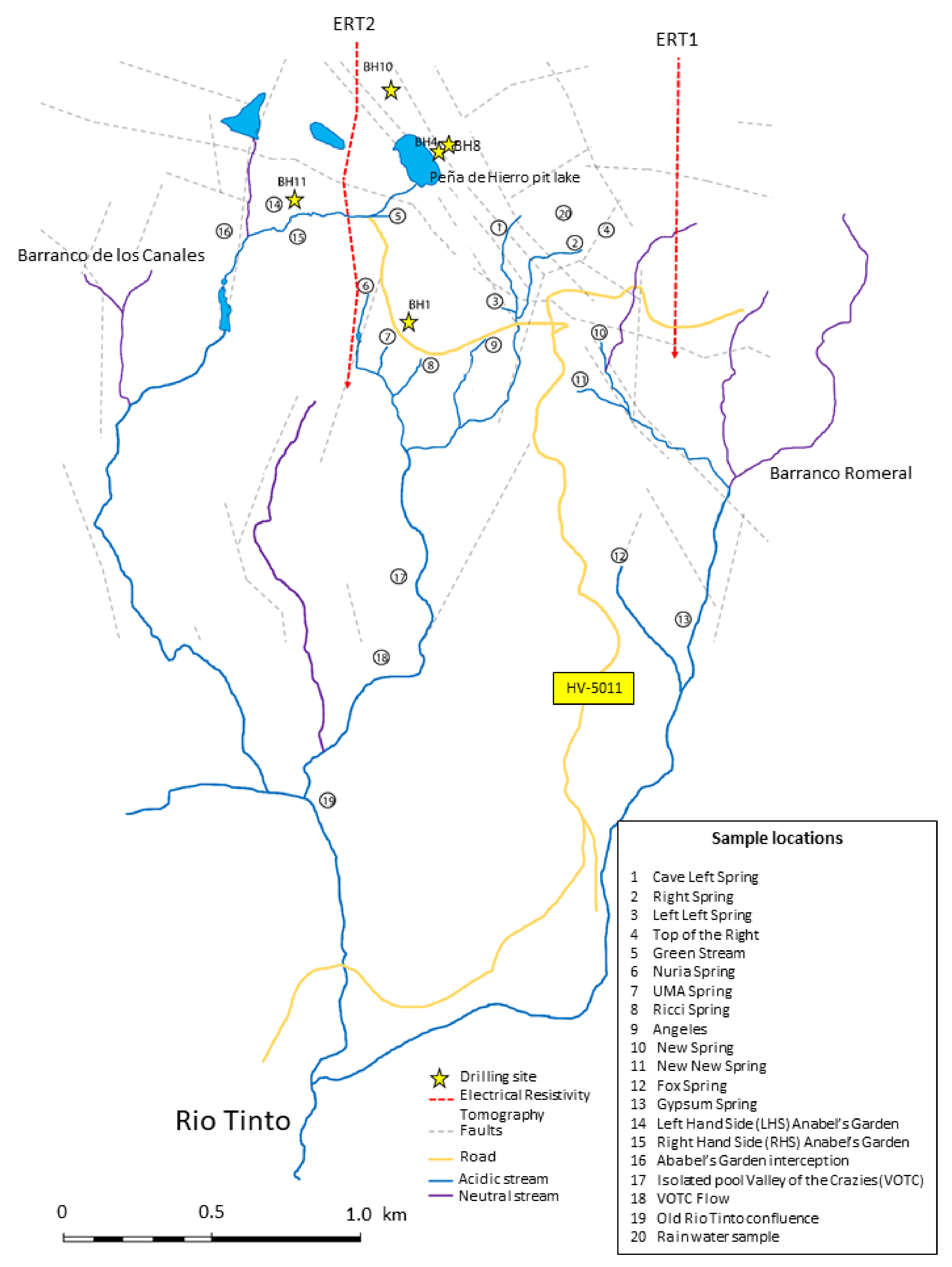
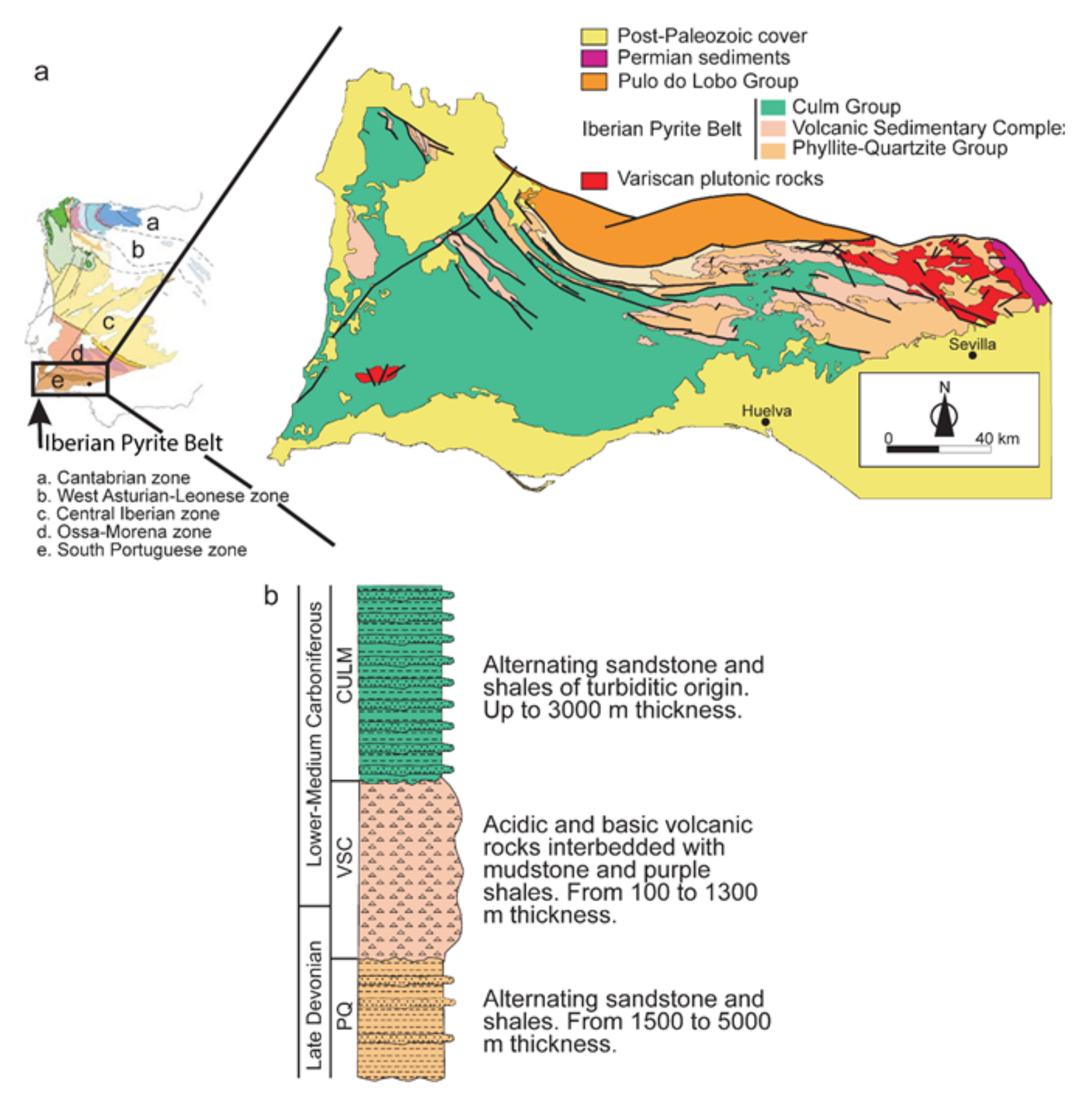
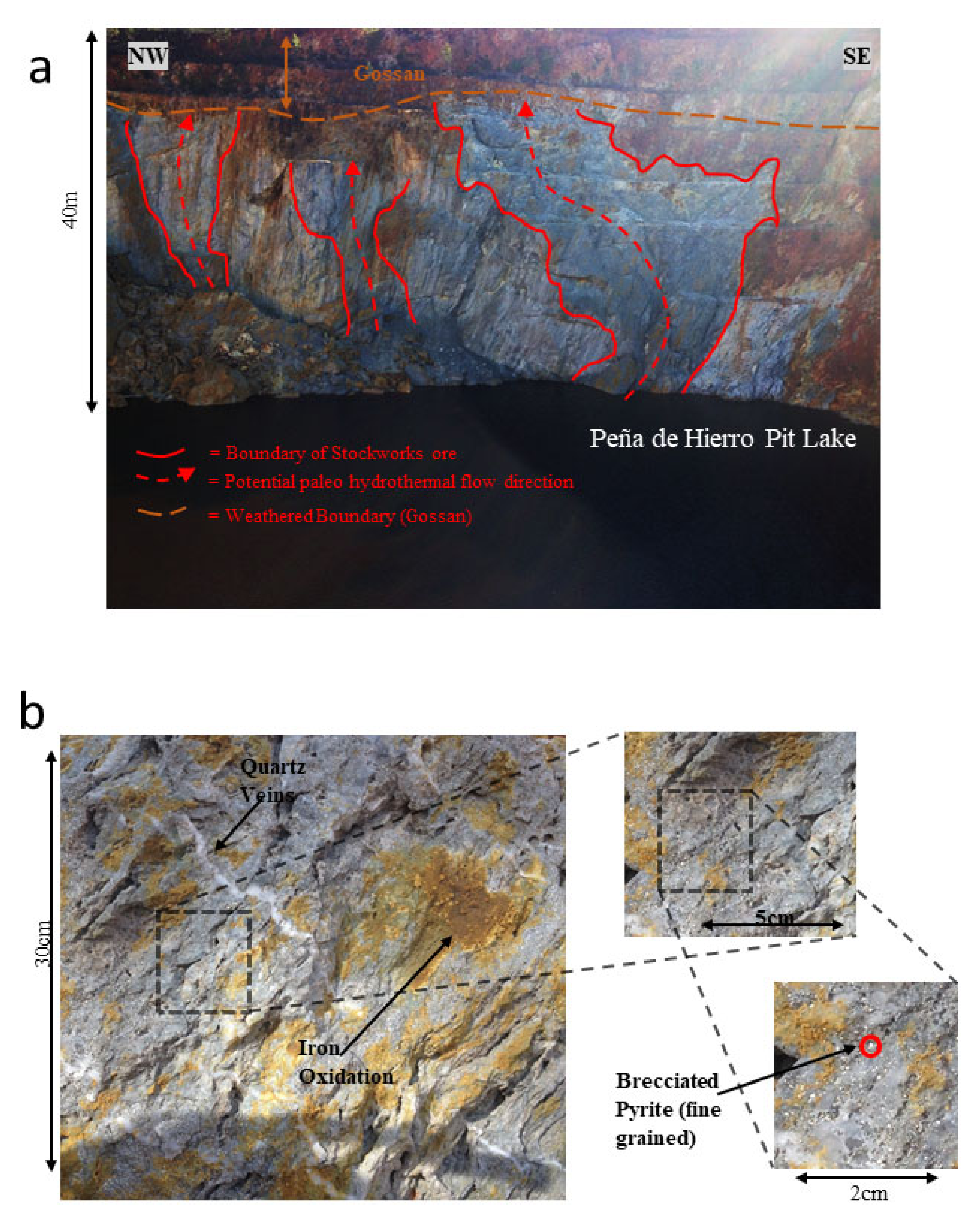
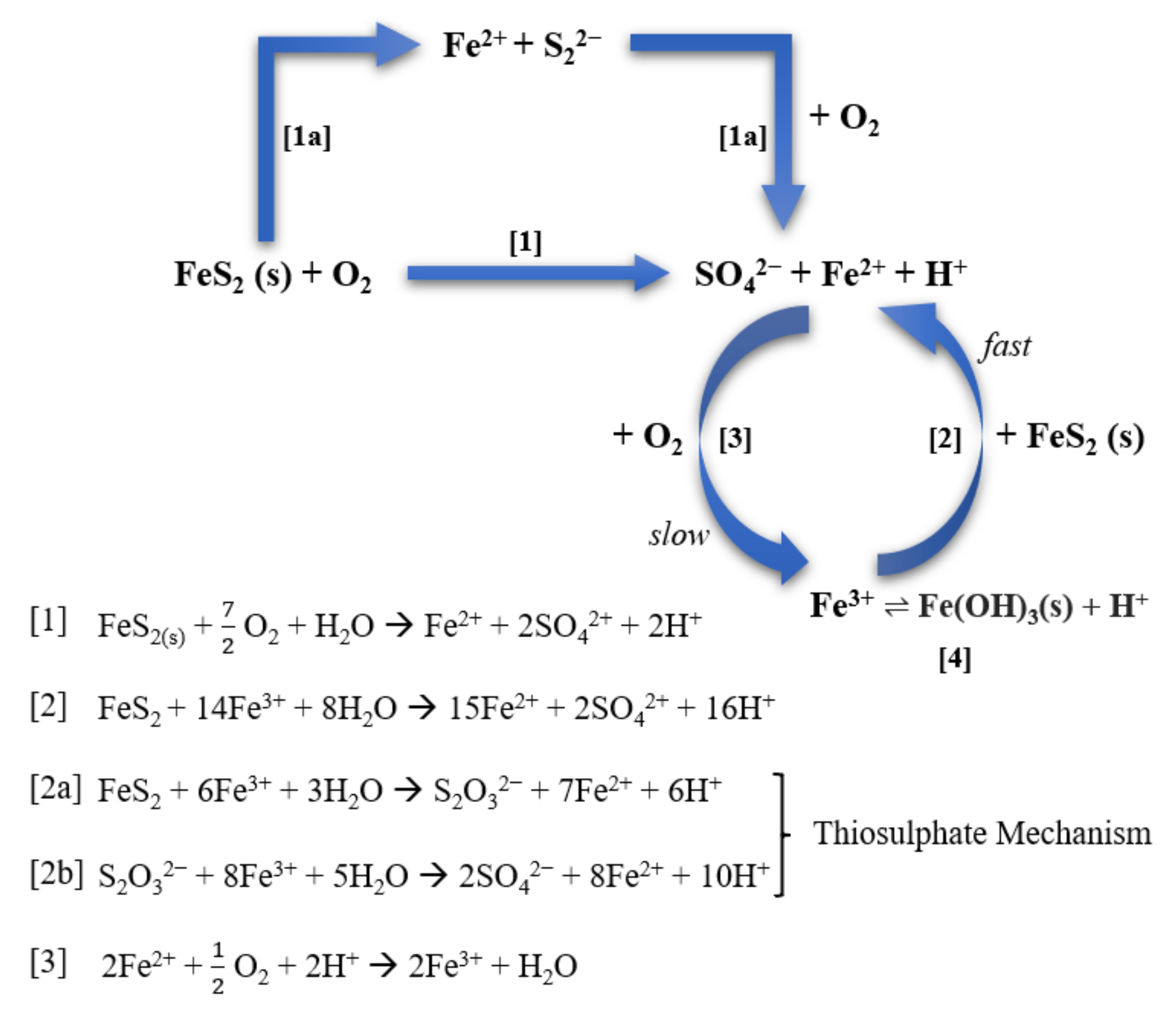
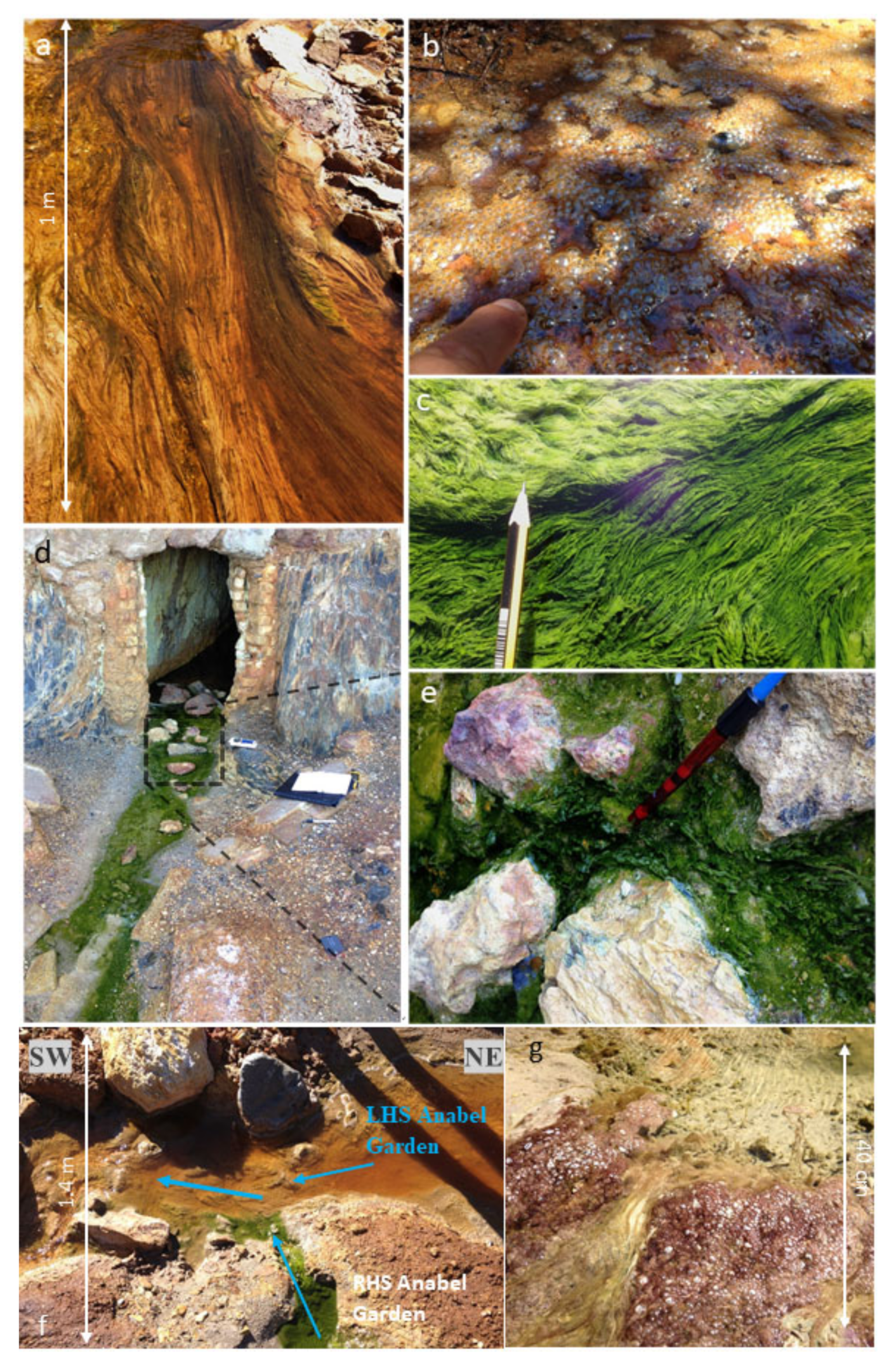
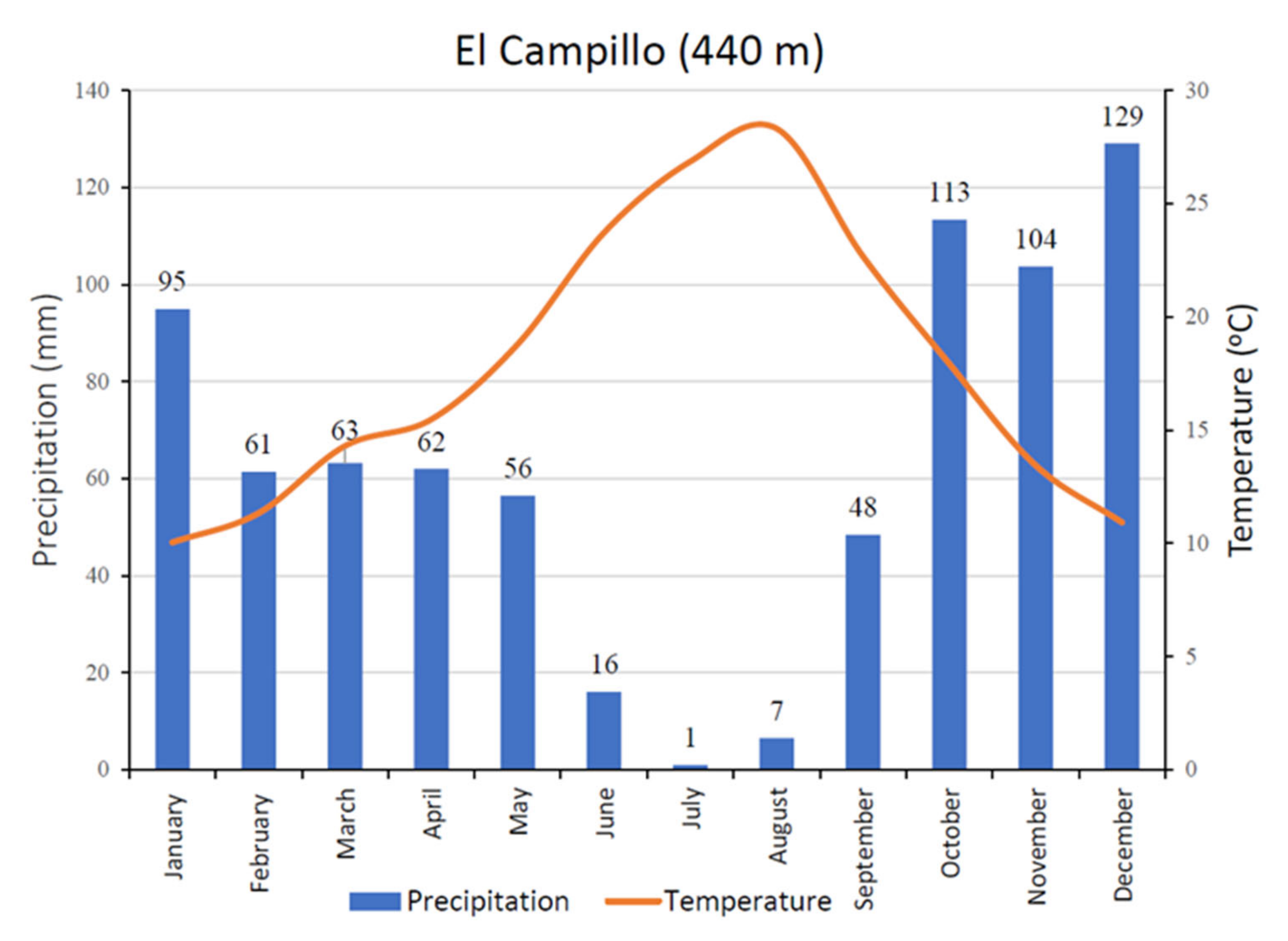
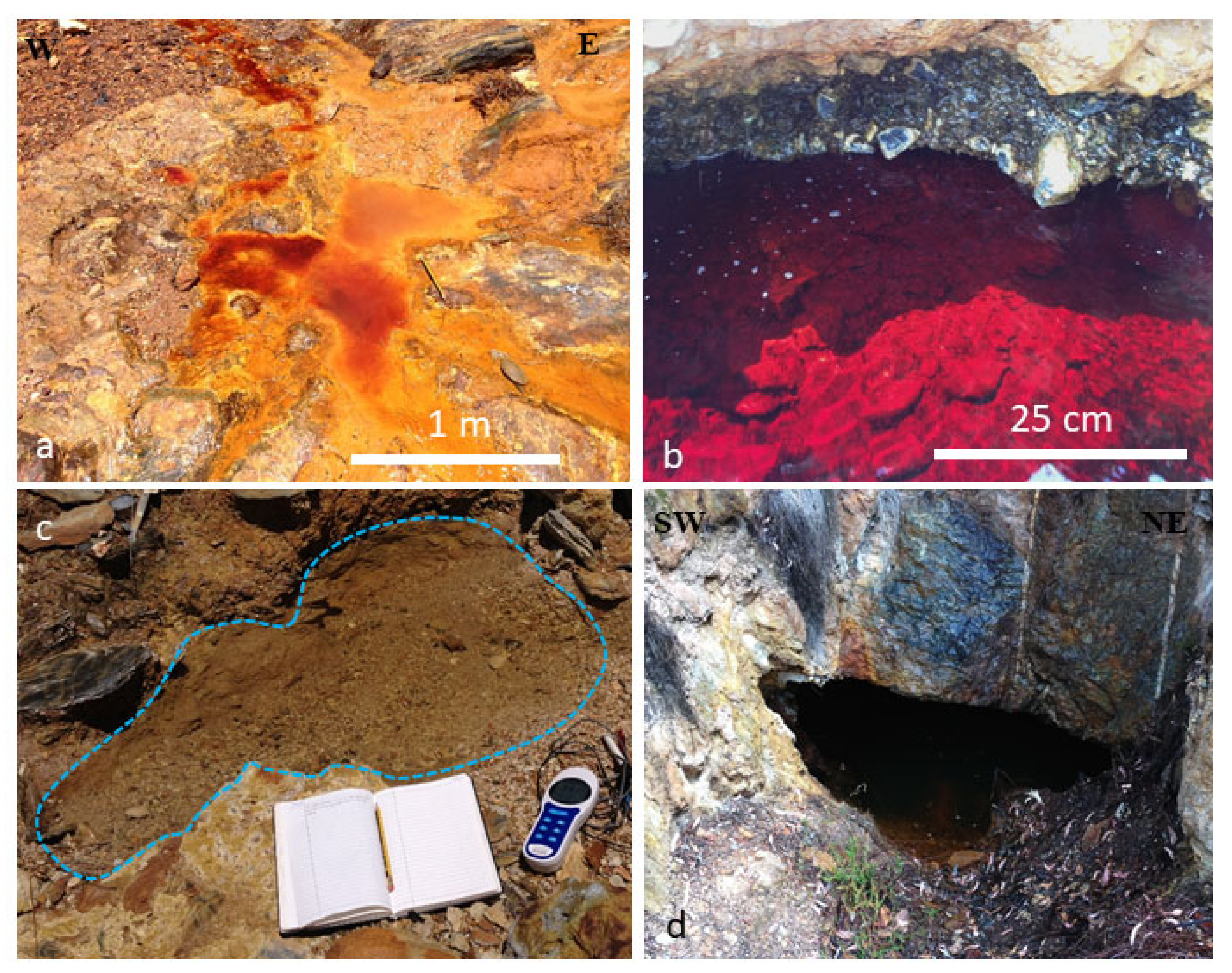
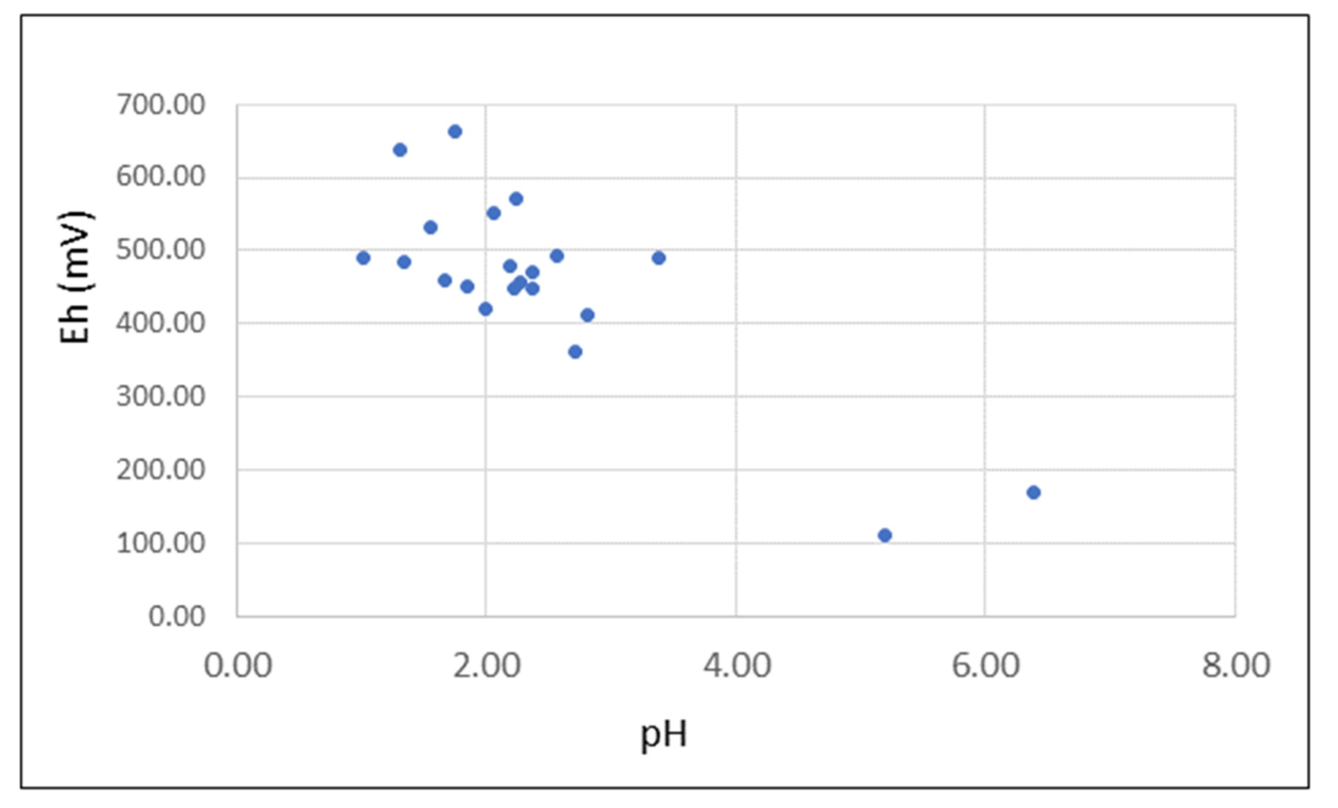
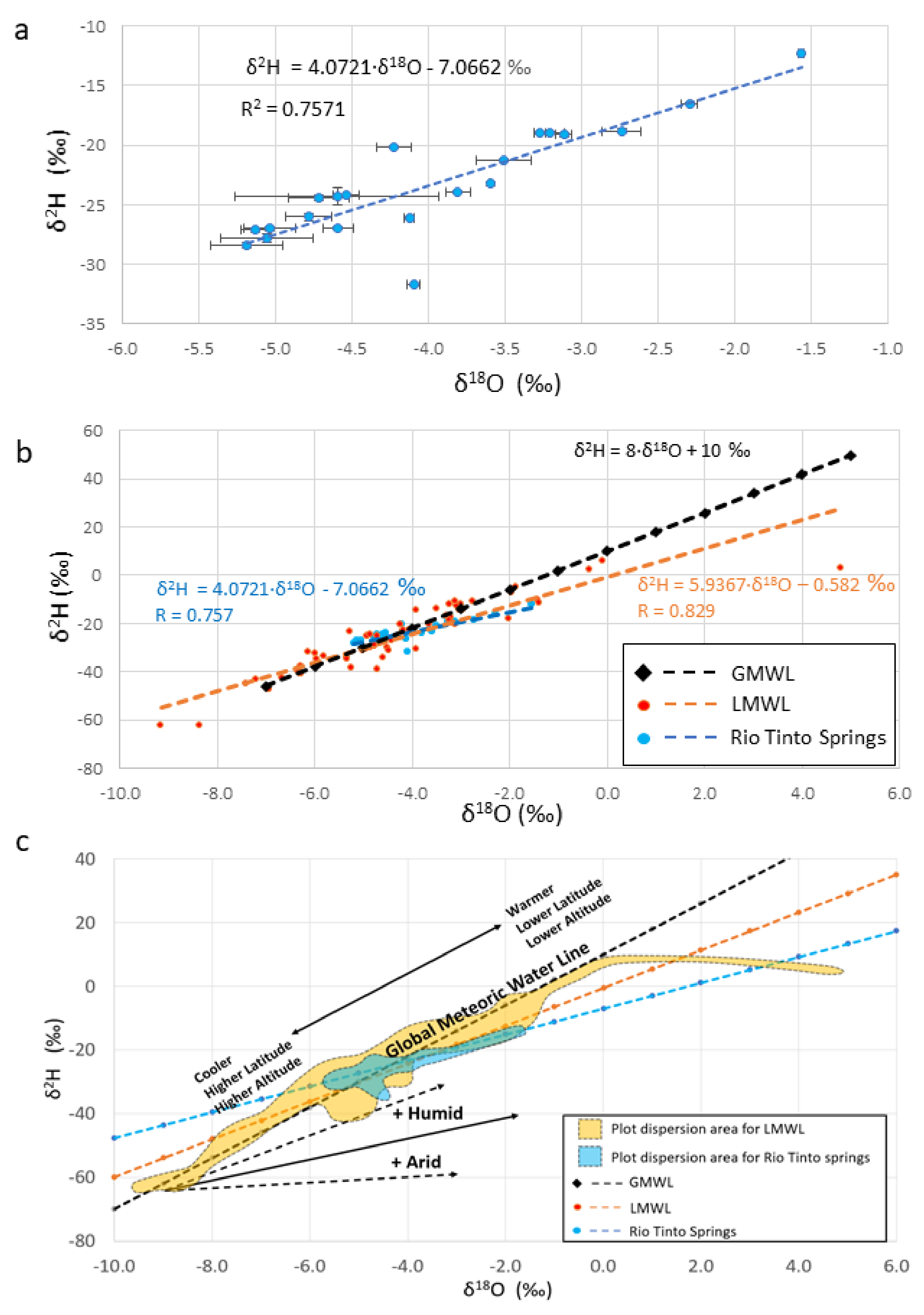
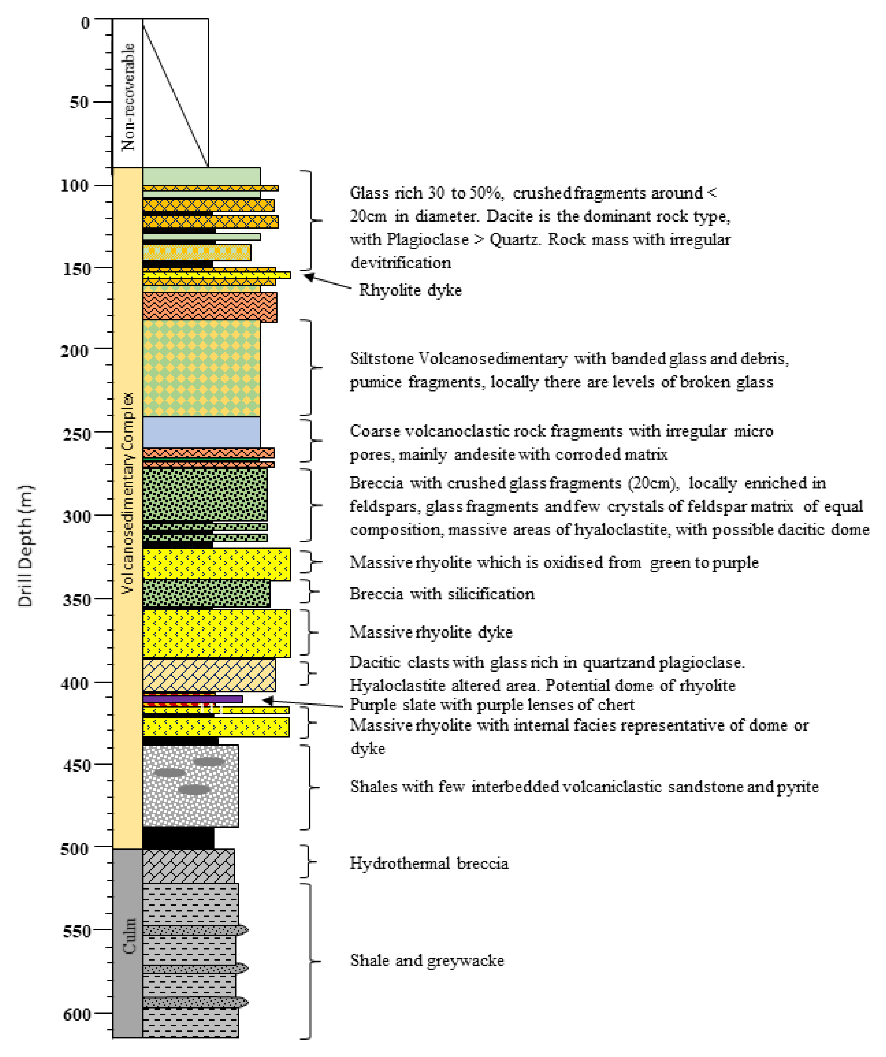
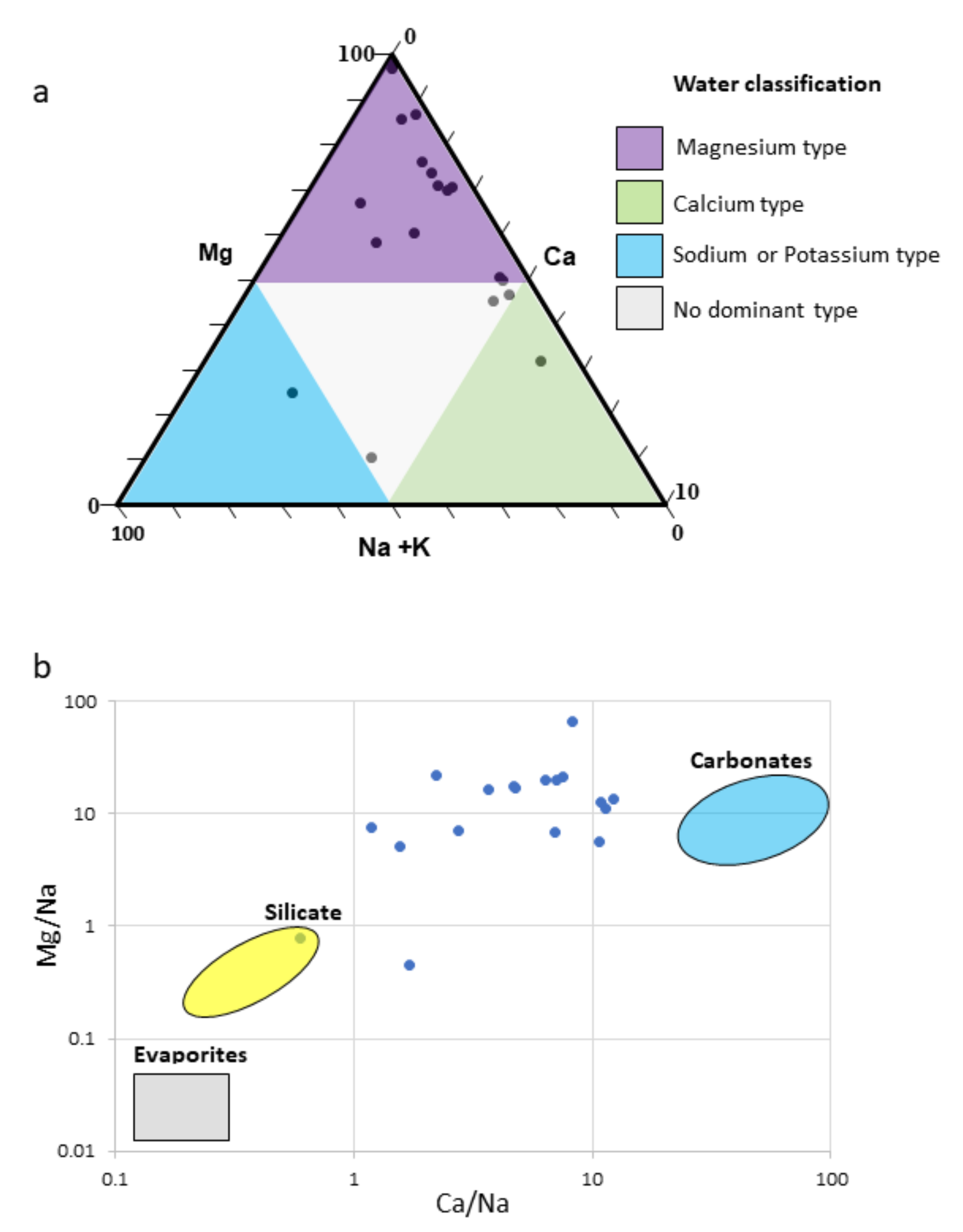
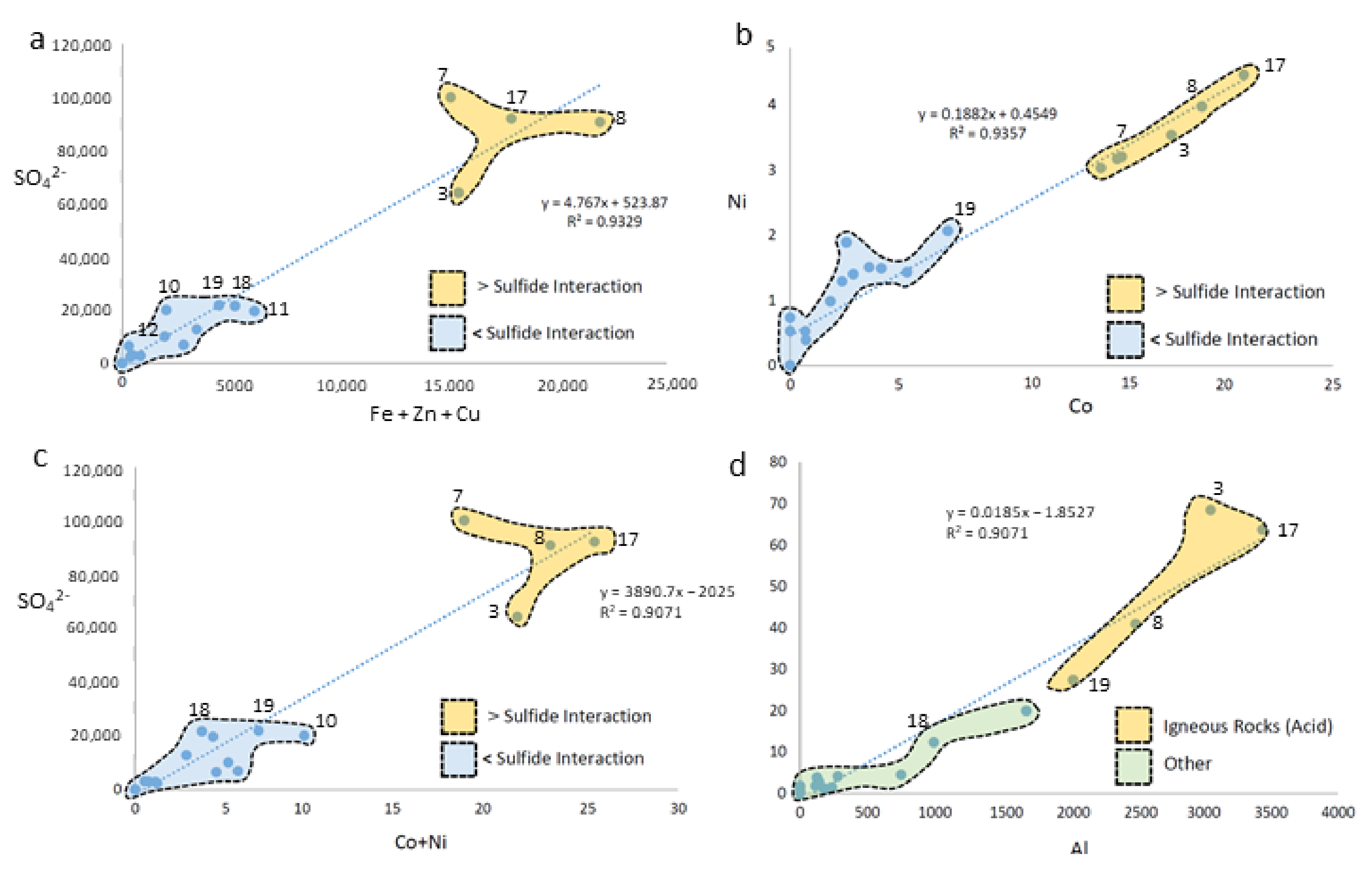
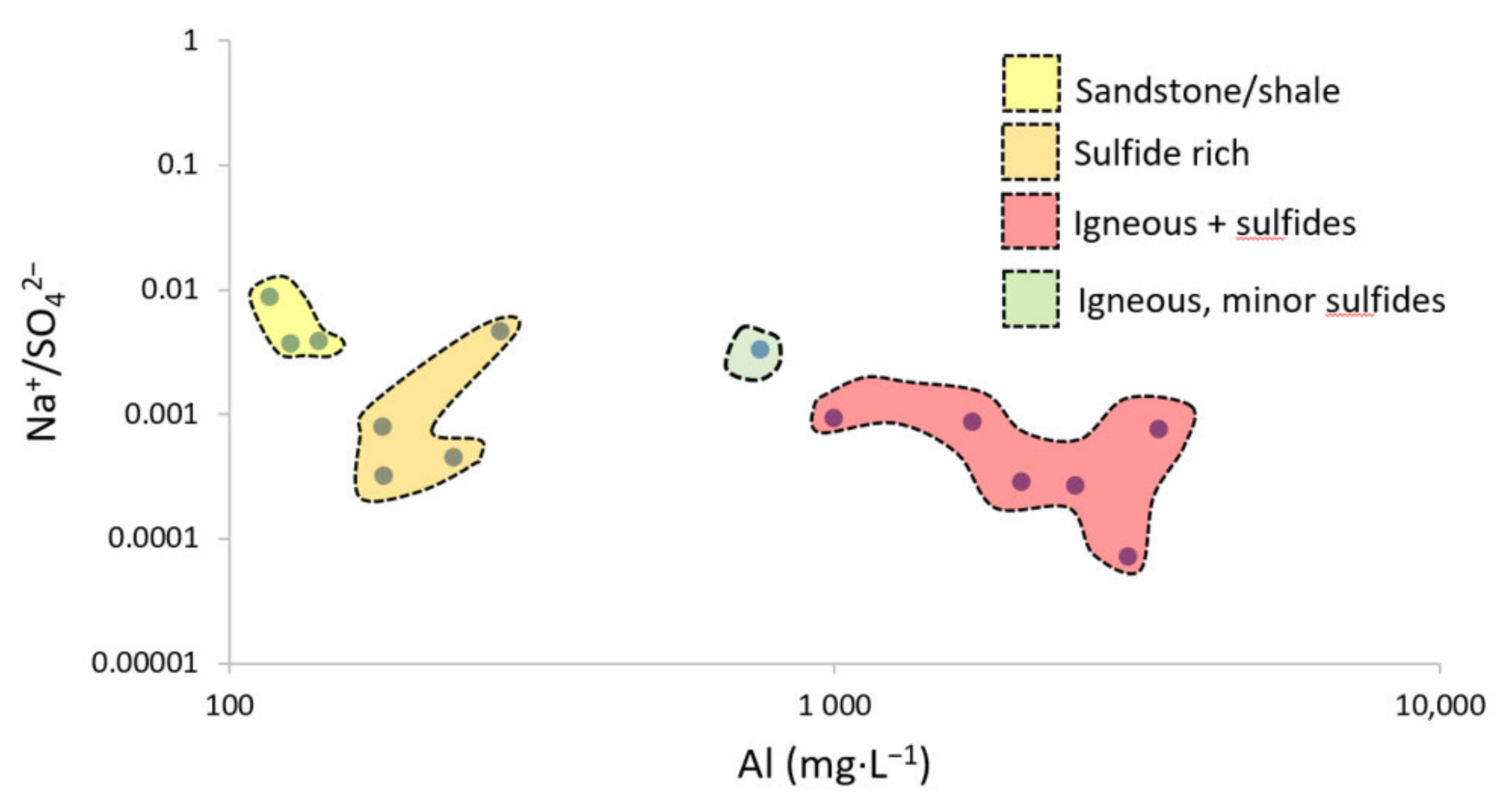
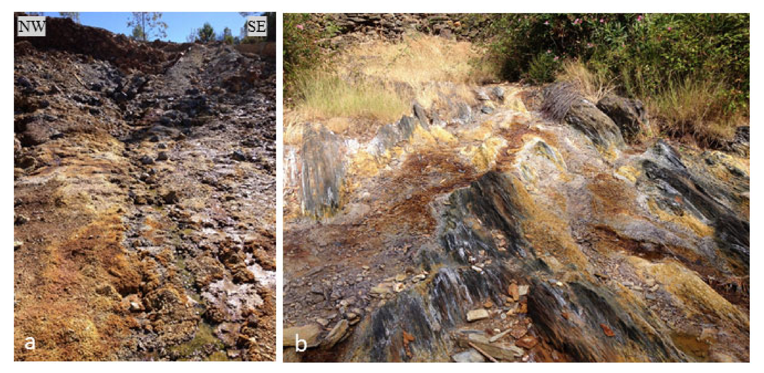
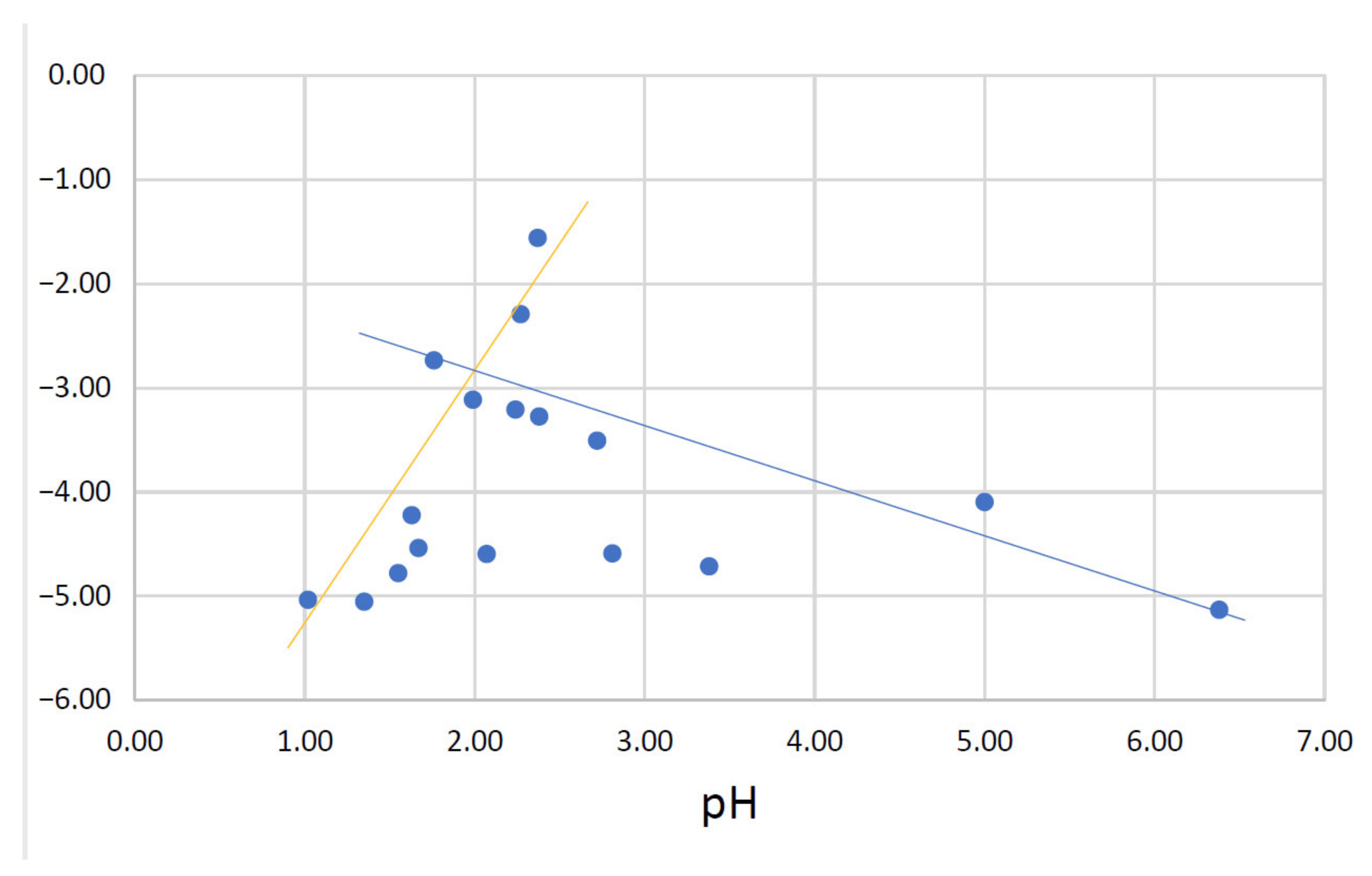
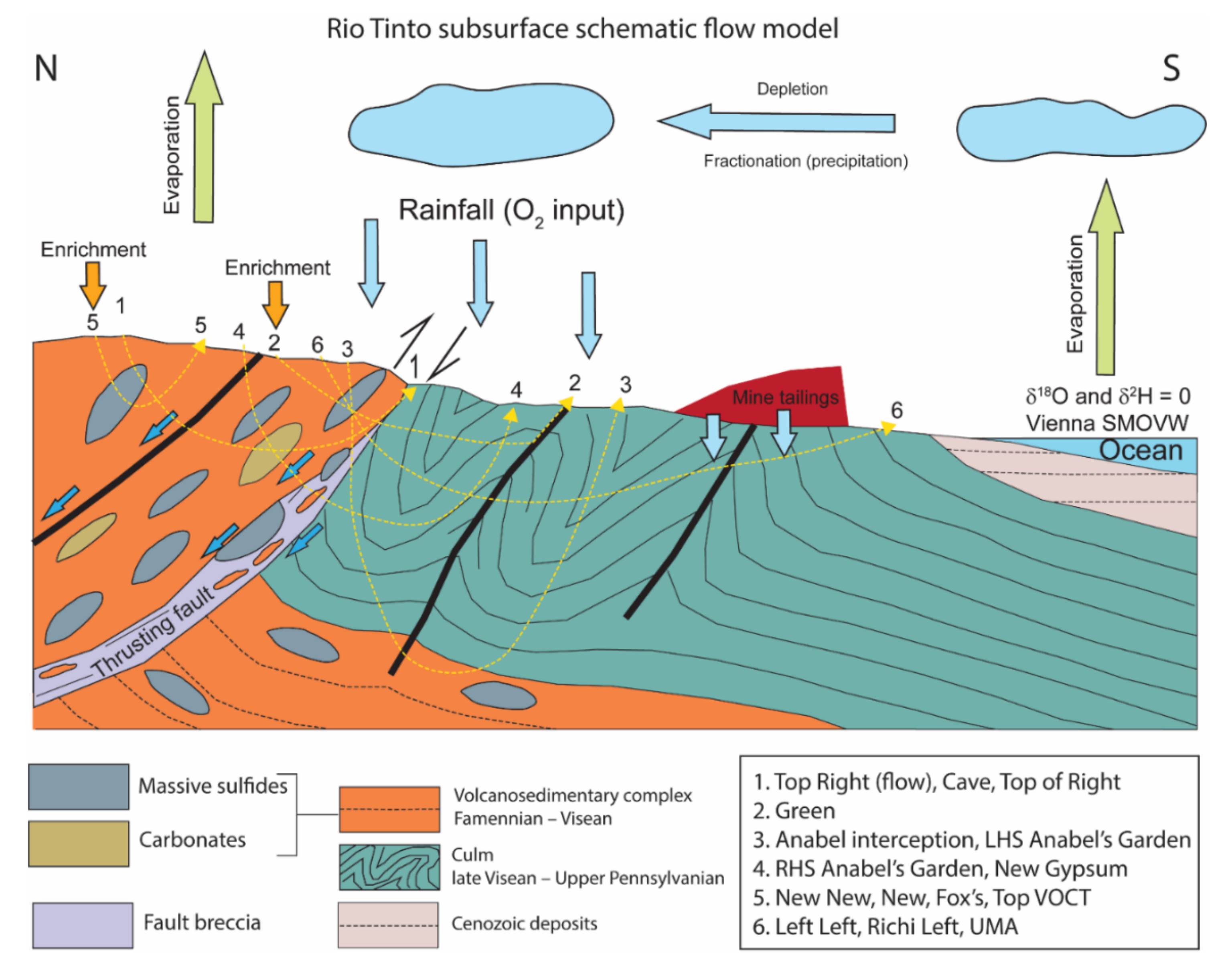
Table 1.
Summary of the spring’s characteristics on a relative scale. Discharge: 1 = not visible; 2 = low; 3 = moderate; 4 = large; 5 = very large. Clarity: 1 = very poor; 2 = slightly cloudy; 3 = moderate; 4 = clear; 5 = excellent clarity. All scales used are on a relative scale (unitless).
Table 1.
Summary of the spring’s characteristics on a relative scale. Discharge: 1 = not visible; 2 = low; 3 = moderate; 4 = large; 5 = very large. Clarity: 1 = very poor; 2 = slightly cloudy; 3 = moderate; 4 = clear; 5 = excellent clarity. All scales used are on a relative scale (unitless).
| Sample Number | Locality | Discharge | Clarity | Color | Deposits/Observations | Biological Activity |
|---|---|---|---|---|---|---|
| 1 | Cave | 1 | 2 | Colorless | None | Absent |
| 2 | Right | 3 | 1 | Pale Orange | Ferrihydrite/”fluffy” orange powder | Brown filamentous algae, oily biofilm, bubbles on surface |
| 2 | Right (pool) | 1 | 2 | Pale Black | None | Absent |
| 3 | Left Left | 2 | 5 | Deep Red/Orange | Orange precipitate | Algae covers in iron oxide |
| 5 | Green Spring | 3 | 5 | Colorless | Copiapite | Light green phototrophic algae + Extracellular Polymeric Substance (EPS) |
| 7 | UMA | 2 | 4 | Deep Orange | None | Dark Green phototrophic algae |
| 8 | Top Ricci | 2 | 5 | Light green | Many Evaporites | Absent |
| 8 | Left Ricci | 2 | 4/5 | Orange | None | Absent |
| 9 | Angels Source | 3 | 5 | Red | Copiapite | Absent |
| 9 | RHS Angeles | 2 | 5 | Yellow/Green | None | Absent |
| 10 | New Spring | 2 | 5 | Pale Fluorescent Green | Copiapite, Sulphur Odor | Bright Green Phototrophic Algae |
| 11 | New New Spring | 2/3 | 5 | Yellow/Green | None | Absent |
| 12 | Suspected Fox’s Spring | 3 | 5 | Colorless | Patches of Copiapite, sulphur odor | Vivid Green phototrophic algae |
| 13 | Gypsum Spring | 2 | 2 | Murky Orange | Gypsum + copiapite | Oily Biofilm |
| 14 | LHS Anabels | 3 | 4 | Orange | Copiapite | Absent |
| 15 | RHS Anabels | 2/3 | 5 | Light Green | Gypsum | Bright green photrophic matts + oily biofilm |
| 16 | Anabel Confluence Spring | 2/3 | 5 | Light Green | Copiapite | Brown/Purple filamentous algae |
| 17 | Top VOTC | 2 | 2 | Deep Red | Copiapite | Absent |
| 18 | VOTC | 2 | 5 | Orange/Red | None | Absent |
| 19 | Old Rio Tinto | 5 | 3 | Faint Orange | None | Absent |
| n/a | Nuria | 3 | 5 | Orange | Copiapite | Long green/brown filamentous Algae |
Table 2.
pH and Eh (mV) of spring and stream solutions.
| Sample Number | Locality | pH | Eh (mV) |
|---|---|---|---|
| 1 | Cave Left | 3.38 | 489.00 |
| 2 | Right | 6.38 | 171.00 |
| 2 | Right (pool) | 5.00 | 110.00 |
| 3 | Left Left | 2.19 | 478.00 |
| 5 | Green Spring | 2.37 | 470.00 |
| 6 | Nuria Spring | 2.57 | 492.00 |
| 7 | UMA | 1.35 | 484.00 |
| 8 | Top Ricci | 1.85 | 452.00 |
| 8 | Left Ricci | 2.07 | 551.00 |
| 9 | Angeles Source | 2.22 | 449.00 |
| 9’ | RHS Angeles | 2.24 | 571.00 |
| 10 | New Spring | 1.55 | 533.00 |
| 11 | New New Spring | 1.02 | 489.00 |
| 12 | Fox’s Spring | 1.67 | 459.00 |
| 13 | Gypsum Spring | 2.81 | 411.00 |
| 14 | LHS Anabel’s Garden | 2.72 | 362.00 |
| 15 | RHS Anabel’s Garden | 1.99 | 420.00 |
| 16 | Anabel Confluence Spring | 2.38 | 449.00 |
| 17 | Top VOTC | 1.32 | 638.00 |
| 18 | VOTC | 1.76 | 662.00 |
| 19 | Old Rio Tinto | 2.27 | 458.00 |
Table 3.
Table summarizing the measured oxygen 18 and deuterium isotopic values on the Picarro L2130-I isotope analyzer situated at The Scottish Association for Marine Science. Each of the values have two standard error values for each locality. Samples were measured using a Picarro L2130-I isotope analyzer (Santa Clara, CA, USA). Each sample was measured 9 times (over 1.5 h) with the first six results ignored due to the potential memory effect of the previous sample. The remaining three results are reported as a mean ratio and an error expressed as two times the standard deviation of the three analysis. Raw isotope ratios were converted delta notation relative to V-SMOW (2) by using certified reference material IA-RO52, IA-RO53 and IA-RO54.
| Sample Location Number | Sample Name | δ18O (‰) | Error 2 σ (‰) | d2H (‰) | Error 2 σ (‰) |
|---|---|---|---|---|---|
| 1 | Cave Left | −4.72 | 0.20 | −24.44 | 0.22 |
| 2 | Top of Right (Flow) | −4.10 | 0.04 | −31.73 | 0.09 |
| 3 | Left Left Stream | −4.22 | 0.11 | −20.16 | 0.11 |
| 4 | Top of Right | −5.13 | 0.10 | −27.11 | 0.20 |
| 5 | Green Stream | −1.56 | 0.02 | −12.29 | 0.04 |
| 7 | UMA Spring | −5.05 | 0.30 | −27.77 | 0.36 |
| 8 | Ricci Left | −4.60 | 0.66 | −24.35 | 0.73 |
| 9 | RHS Angeles | −3.21 | 0.10 | −18.89 | 0.10 |
| 9 | Angeles Source | −5.19 | 0.24 | −28.38 | 0.22 |
| 10 | Top New Spring | −4.78 | 0.15 | −26.00 | 0.31 |
| 11 | New New Spring | −5.04 | 0.17 | −27.01 | 0.17 |
| 12 | Fox Spring | −4.54 | 0.08 | −24.17 | 0.03 |
| 13 | New Gypsum Spring | −4.59 | 0.10 | −26.97 | 0.16 |
| 14 | LHS Anabel’s Garden | −3.51 | 0.18 | −21.28 | 0.13 |
| 15 | RHS Anabel’s Garden | −3.12 | 0.05 | −19.11 | 0.18 |
| 16 | Anabel Interception | −3.28 | 0.04 | −18.94 | 0.09 |
| 18 | Flow VOTC | −2.74 | 0.13 | −18.77 | 0.17 |
| 17 | Top VOTC | 17.43 | 0.36 | 46.16 | 0.60 |
| 19 | Old Rio Tinto Confluence | −2.29 | 0.05 | −16.48 | 0.08 |
| 20 | Rain Water Stream | −4.13 | 0.03 | −26.12 | 0.14 |
| n/a | Rain Water Folder (1) | −3.81 | 0.08 | −23.96 | 0.11 |
| n/a | Rain Water Folder (2) | −3.60 | 0.01 | −23.25 | 0.18 |
Table 4.
Element list of cations (mg∙L−1) obtained through ICP (Induced Couple Plasma) geochemical analysis.
Table 4.
Element list of cations (mg∙L−1) obtained through ICP (Induced Couple Plasma) geochemical analysis.
| Locality Number | Locality | Al | As | Ca | Cd | Co | Cu | Fe | K | Mg | Mn | Na | Ni | Si | Zn |
|---|---|---|---|---|---|---|---|---|---|---|---|---|---|---|---|
| 1 | Cave Left | 0.00 | 0.00 | 7.20 | 0.00 | 0.00 | 0.00 | 0.00 | 8.70 | 9.30 | 0.00 | 12.00 | 0.00 | 14.40 | 0.00 |
| 2 | Top of Right—right spring | 0.00 | 0.00 | 369.90 | 0.00 | 0.00 | 0.00 | 499.40 | 9.00 | 407.00 | 99.40 | 30.30 | 0.70 | 5.70 | 5.70 |
| 3 | Left Left Stream | 3053.10 | 13.00 | 18.70 | 0.50 | 17.60 | 15.70 | 15,428.80 | 7.20 | 1728.30 | 29.00 | 4.60 | 3.50 | 66.80 | 13.40 |
| 4 | Top of Right | 0.00 | 0.00 | 16.10 | 0.00 | 0.00 | 0.00 | 0.00 | 9.60 | 4.20 | 2.90 | 9.40 | 0.00 | 1.20 | 0.00 |
| 5 | Green Stream | 140.40 | 2.60 | 71.50 | 0.00 | 0.70 | 8.20 | 818.40 | 8.10 | 222.10 | 13.60 | 11.30 | 0.40 | 42.10 | 29.20 |
| 7 | UMA Spring (1) | 2044.60 | 24.50 | 138.40 | 0.80 | 15.10 | 74.10 | 15,200.60 | 8.80 | 506.70 | 26.90 | 29.30 | 3.20 | 72.50 | 111.50 |
| 7 | UMA Spring (2) | 1914.20 | 23.40 | 128.40 | 0.80 | 14.30 | 68.50 | 14,224.10 | 8.70 | 464.50 | 25.30 | 27.00 | 3.00 | 68.60 | 105.30 |
| 7 | UMA Spring (3) | 2062.00 | 24.90 | 135.90 | 0.80 | 15.30 | 74.20 | 14,952.90 | 8.70 | 501.70 | 26.90 | 29.70 | 3.20 | 73.20 | 112.70 |
| 8 | Ricci Left | 2494.70 | 37.70 | 54.50 | 1.00 | 19.00 | 107.40 | 21,767.90 | 9.60 | 543.50 | 26.40 | 24.40 | 4.00 | 59.70 | 82.90 |
| 9 | RHS Ángeles | 751.70 | 2.50 | 81.00 | 0.00 | 2.60 | 9.70 | 288.20 | 7.70 | 354.90 | 33.50 | 22.00 | 1.90 | 86.90 | 19.00 |
| 10 | Top New Spring | 235.50 | 32.00 | 26.70 | 0.00 | 2.40 | 31.20 | 5149.60 | 7.80 | 67.70 | 11.90 | 9.70 | 1.30 | 54.10 | 7.60 |
| 11 | New New Spring | 180.40 | 40.80 | 7.60 | 0.00 | 2.90 | 81.40 | 5991.10 | 9.80 | 48.70 | 7.50 | 6.40 | 1.40 | 60.10 | 12.30 |
| 12 | Fox Spring | 179.10 | 12.50 | 16.40 | 0.00 | 1.90 | 30.80 | 3390.50 | 11.50 | 53.80 | 6.90 | 10.50 | 1.00 | 60.60 | 7.70 |
| 13 | New Gypsum Spring | 0.00 | 0.00 | 562.70 | 0.00 | 0.00 | 0.00 | 426.60 | 8.60 | 297.00 | 47.80 | 52.70 | 0.50 | 6.50 | 2.00 |
| 14 | LHS Anabel’s Garden | 126.10 | 2.60 | 436.60 | 0.00 | 3.60 | 19.00 | 1821.20 | 7.80 | 426.90 | 169.50 | 38.40 | 1.50 | 57.00 | 126.40 |
| 15 | RHS Anabel’s Garden | 279.80 | 4.70 | 354.90 | 0.00 | 4.20 | 24.90 | 2690.30 | 8.80 | 407.80 | 144.60 | 32.50 | 1.50 | 43.50 | 115.10 |
| 16 | Anabel Interception | 116.20 | 2.40 | 150.50 | 0.00 | 0.70 | 11.00 | 328.90 | 7.80 | 149.40 | 45.80 | 21.50 | 0.50 | 48.40 | 32.30 |
| 17 | Top VOTC | 3438.90 | 21.20 | 517.60 | 1.10 | 20.90 | 125.80 | 17,579.20 | 7.20 | 1447.30 | 115.80 | 69.10 | 4.50 | 157.80 | 177.50 |
| 18 | Flow VOTC | 994.00 | 3.90 | 145.90 | 0.00 | 5.40 | 29.10 | 4384.60 | 7.60 | 407.60 | 34.50 | 20.40 | 1.40 | 56.50 | 41.50 |
| 19 | Old Rio Tinto Confluence | 1682.50 | 5.50 | 145.60 | 1.10 | 7.30 | 322.70 | 1479.40 | 10.90 | 1166.60 | 95.60 | 17.70 | 2.10 | 54.20 | 231.60 |
| 20 | Rainwater Stream | 0.00 | 0.00 | 5.00 | 0.00 | 0.00 | 0.00 | 0.00 | 9.00 | 0.00 | 0.00 | 6.20 | 0.00 | 0.00 | 0.00 |
| Rainwater Flow (1) | 0.00 | 0.00 | 4.00 | 0.00 | 0.00 | 0.00 | 0.00 | 10.30 | 0.00 | 0.00 | 5.30 | 0.00 | 0.00 | 0.00 | |
| Rainwater Flow (2) | 0.00 | 0.00 | 5.50 | 0.00 | 0.00 | 0.00 | 0.00 | 10.40 | 0.00 | 0.00 | 5.60 | 0.00 | 0.00 | 0.50 | |
| Element total concentration | 19,693.2 | 254.2 | 3400.6 | 6.1 | 133.9 | 1033.7 | 126,421.7 | 203.6 | 9215 | 963.8 | 496 | 35.6 | 1089.8 | 1234.2 |
Table 5.
Anion water composition (mg∙L−1) obtained through ion chromatography of the sample solutions.
Table 5.
Anion water composition (mg∙L−1) obtained through ion chromatography of the sample solutions.
| Locality Number | Locality | F− | Cl− | NO2− | Br− | NO3− | SO42− | PO43− | Spring Total Concentration |
|---|---|---|---|---|---|---|---|---|---|
| 1 | Cave Left | 0.35 | 8.31 | 0 | 0 | 0 | 176.14 | 0 | 184.8 |
| 2 | Right Stream (pool) | 0 | 6.75 | 0 | 0 | 0 | 50.46 | 0 | 57.21 |
| 3 | Left Left | 68.52 | 2.76 | 0 | 0 | 0 | 64,547.85 | 0 | 64,619.13 |
| 4 | Right Stream—Top of Right | 1.83 | 3.76 | 0 | 0 | 0 | 3088.09 | 7.8 | 3101.48 |
| 5 | Green Stream | 2.82 | 5.12 | 0 | 0 | 0 | 2913.09 | 23.91 | 2944.94 |
| 7 | UMA Spring | 27.4 | 1.66 | 0 | 0 | 0 | 100,546.59 | 2.43 | 100,578.08 |
| 8 | Ricci Left | 41.02 | 2.34 | 0 | 0 | 0 | 91,214.69 | 3.56 | 91,261.61 |
| 9 | RHS Ángeles | 4.53 | 2.74 | 0 | 0 | 1.79 | 6584.3 | 0 | 6593.36 |
| 10 | Top New Spring | 1.51 | 2.38 | 0 | 0 | 0 | 21,780.05 | 0 | 21,783.94 |
| 11 | New New Spring | 1.23 | 1.59 | 0 | 0 | 0 | 19,812.78 | 0 | 19,815.6 |
| 12 | Fox Spring | 1.07 | 3.69 | 0 | 0 | 0 | 12,935.9 | 0 | 12,940.66 |
| 13 | New Gypsum Spring | 0.71 | 6.11 | 0 | 0 | 0 | 3127.21 | 0 | 3134.03 |
| 14 | LHS Anabel’s Garden | 3.84 | 7.61 | 0 | 0 | 0 | 10,204.99 | 0 | 10,216.44 |
| 15 | RHS Anabel’s Garden | 4.18 | 8.56 | 0 | 0 | 0 | 6981.06 | 0 | 6993.8 |
| 16 | Anabel Interception | 1.85 | 10.5 | 0 | 0 | 0 | 2452.61 | 0 | 2464.96 |
| 18 | Flow VOTC | 12.41 | 6.31 | 0 | 0 | 2.88 | 22,003.87 | 0 | 22,025.47 |
| 17 | Top VOTC | 63.77 | 38.51 | 0 | 0 | 45.02 | 92,550.55 | 3.06 | 92,700.91 |
| 19 | Old Rio Tinto Confluence (1) | 25.85 | 18.24 | 0 | 0 | 16.98 | 26,046.91 | 0 | 26,107.98 |
| 19 | Old Rio Tinto Confluence (2) | 19.31 | 14.25 | 0 | 0 | 13.31 | 19,506.98 | 0 | 19,553.85 |
| 19 | Old Rio Tinto Confluence | 18.04 | 13.75 | 0 | 0 | 13.02 | 18,224.2 | 4.66 | 18,273.67 |
| Rain Water Folder | 0 | 4.36 | 0 | 0 | 0 | 76.73 | 0 | 81.09 | |
| Rain Water Folder | 0 | 3.65 | 0 | 0 | 0 | 123.68 | 3.18 | 130.51 | |
| Anion total concentration | 300.24 | 172.95 | 0 | 0 | 93 | 524,948.73 | 48.6 |
Publisher’s Note: MDPI stays neutral with regard to jurisdictional claims in published maps and institutional affiliations. |
© 2021 by the authors. Licensee MDPI, Basel, Switzerland. This article is an open access article distributed under the terms and conditions of the Creative Commons Attribution (CC BY) license (https://creativecommons.org/licenses/by/4.0/).
Share and Cite
MDPI and ACS Style
Allman, C.J.; Gómez-Ortiz, D.; Burke, A.; Amils, R.; Rodriguez, N.; Fernández-Remolar, D. Hydrogeochemical Variability of the Acidic Springs in the Rio Tinto Headwaters. Water 2021, 13, 2861. https://doi.org/10.3390/w13202861
AMA Style
Allman CJ, Gómez-Ortiz D, Burke A, Amils R, Rodriguez N, Fernández-Remolar D. Hydrogeochemical Variability of the Acidic Springs in the Rio Tinto Headwaters. Water. 2021; 13(20):2861. https://doi.org/10.3390/w13202861
Chicago/Turabian StyleAllman, Christopher John, David Gómez-Ortiz, Andrea Burke, Ricardo Amils, Nuria Rodriguez, and David Fernández-Remolar. 2021. "Hydrogeochemical Variability of the Acidic Springs in the Rio Tinto Headwaters" Water 13, no. 20: 2861. https://doi.org/10.3390/w13202861
Note that from the first issue of 2016, this journal uses article numbers instead of page numbers. See further details here.