
Calibration of CFD Numerical Model for the Analysis of a Combined Caisson


1
Department of Engineering, University of Messina, Contrada di Dio, Sant’Agata, 98166 Messina, Italy
2
Department of Civil Engineering and Architecture, University of Catania, Via Santa Sofia, 95123 Catania, Italy
*
Author to whom correspondence should be addressed.
Water 2021, 13(20), 2862; https://doi.org/10.3390/w13202862
Submission received: 2 September 2021
/
Revised: 1 October 2021
/
Accepted: 8 October 2021
/
Published: 13 October 2021
(This article belongs to the Special Issue Wave-Driven Processes in the Coastal Zones)
Abstract
:The purpose of this work is the calibration of a numerical model for simulating the interaction of waves with a composite caisson having an internal rubble mound to dissipate incident sea wave energy. In particular, the analysis focused on the reflection coefficient and the pressure distribution at the caisson vertical walls. The numerical model is based on the Volume-Average Reynolds-Averaged Navier–Stokes (VARANS) equations. Through three closure terms (linear, nonlinear, and transition), such equations take into account some phenomena that cannot be dealt when the volume-average method is used (i.e., frictional forces, pressure force, and added mass). To reproduce properly the real phenomena, a calibration process of such terms is necessary. The reference data used in the calibration process were obtained from an experimental campaign carried out at the Hydraulics Laboratory of the University of Messina. The calibration process allowed the proper prediction of certain phenomena to be expressed as a function of different closing terms. In particular, it was estimated that the reflection coefficient and the wave loading at the frontal wall are better reproduced when all three terms are considered, while the force at the rear wall is better simulated when the effects of such terms are neglected.
1. Introduction
In the last decades, the increase in the volume of transported goods and the construction of ships with larger load capacities made it necessary to expand and adapt several port structures. In this regard, one of the biggest challenges in the design phase to improve the efficiency of port operations is the reduction of residual wave energy inside a harbor basin. Therefore, it is important to develop structures that allow the wave reflection to be reduced. On the other hand, the development of a tool capable to predict the efficacy of anti-reflective structures is consequential [1].
One example is provided by structures known as porous caisson sea walls. In these types of structures, the quay is built on piles and the energy dissipation function is entrusted to an absorbing slope composed of armored units arranged around the piles. The disadvantage of these types of structures is basically the large required spaces [2]. In some cases, this disadvantage can be overcome through the realization of perforated caissons. However, in such latter case, a reduction in the dissipation performance is observed [3].
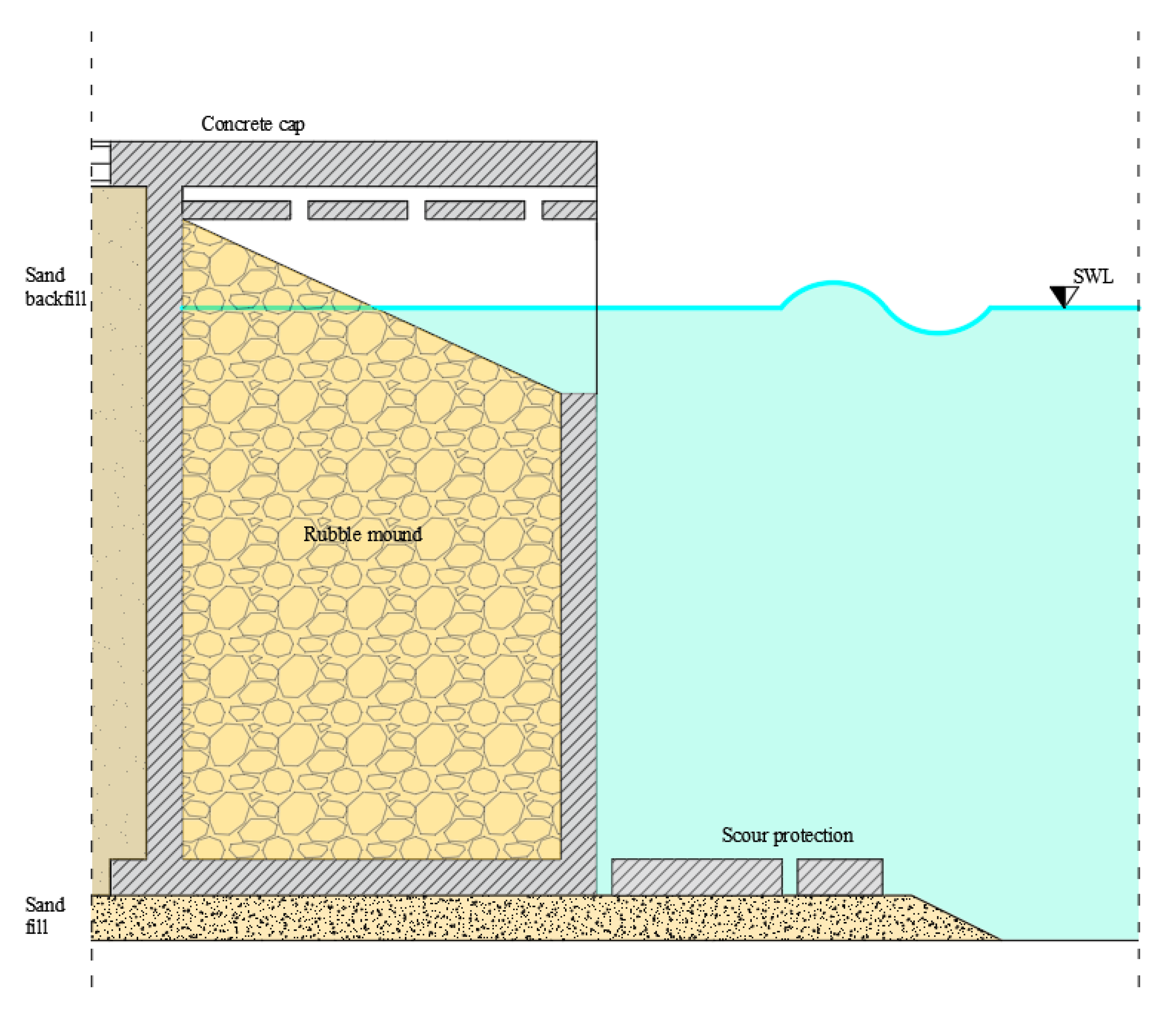
The combination of the aforementioned types of caissons led to propose so called combined caissons, having windowed walls and an internal rubble beach (see Figure 1). This type of caisson allows the energy of the wave motion to be reduced, occupying small spaces.
In the literature there are few studies on combined caissons. Among these, Altomare and Gironella [4] proposed a new formula for evaluating the reflection coefficient on prefabricated caissons with frontal opening and internal rubble mound, and the effects of the model scale on wave reflection were also investigated. Some experiments were carried out by Faraci et al. [5] aimed at finding the reflective response of the structure, while Liu and Faraci [6] developed a semi-analytical model to analyze the reflection of the incident wave. The previously cited studies examined the reflection coefficients of composite caissons and similar structures, but few are aimed at evaluating the stability of such structures.
Faraci and Liu [7], using the semi-analytical model of Liu and Faraci [6], determined the horizontal forces acting on the combined caisson due to the wave motion. The results of the proposed model were validated through a numerical solution obtained by the multi-domain boundary element method (BEM). However, such a type of model implies some simplifications, especially in the simulation of the interaction of waves with the internal rubble mound, which can lead to different results with respect to the real ones.
In the last years, several studies were carried out to properly simulate the interaction of the wave with the porous media. However, most of these studies are based on equations that require the calibration of some parameters. In this regard, the present analysis is devoted at studying the caisson behaviour through a numerical model in order to develop a tool for the performance prediction of the composite caisson. In particular, the main objective of this study is the calibration of a numerical model to estimate the reflection coefficient and the pressures distribution on the combined caisson vertical walls. The calibration process was carried out through the data acquired within an experimental campaign carried out on a scale model of a combined caisson at the Hydraulic Laboratory of the University of Messina.
This study was carried out by the finite-volume-based open-source software OpenFOAM® which has a large user base across most engineering and science areas. In particular, to simulate the interaction between wave and the porous media into composite caisson, in this study the toolbox olaflow was used [8]. This toolbox is based on the Volume-average Reynolds-averaged Navier–Stokes (VARANS) equations [9] using the version proposed by del Jesus et al. [10]. In order to take into account the effects due to phenomena that cannot be dealt when the volume-average method is used (i.e., frictional forces, pressure force, and added mass), the calibration of some coefficients is required. Following Darcy [11], Forchheimer [12], and Polubarinova-Koch [13], the closure terms, which represent the drag and the inertia forces due to the porous media, can be defined by the following relationship known as the extended Forchheimer equation [14]:
where I is the hydraulic gradient; u is the pore velocity; and a, b, and c are porosity or pressure-drop coefficients [15]. The first linear term is the hydraulic gradient for laminar flow, i.e., when the inertia force effects are negligible [11]. The second term accounts the effects of the turbulent flow [12]. The last time-dependent term accounts for the acceleration of the fluid through the porous media [13]. The first two terms represent the drag forces, while the last term refer to the inertia force.
In accordance with the definition of Engelund [16], modified by Van Gent [17], the first two coefficients are defined by the following relationships:
where n is the porosity (the ratio of the pore volume to the total volume), is the kinematic fluid viscosity, mean grain diameter of porous media, and is the Keulegan–Carpenter number. The coefficients , , and c are coefficients that must be determined experimentally for different types of porous media materials [18]. The coefficient c, according to previous works, can be kept constant. In particular, a suggested value is equal to 0.34 [10,14,17].
Previous studies estimated the values of these coefficients for some types of coastal structures. An extensive analysis is presented by Losada et al. [19]. Some studies useful to justify the choice of the coefficients adopted in this article are here discussed.
In the study conducted by Van Gent [20] on coastal structures, the values of and were imposed equal to 1000 and 1.1, respectively. These values were also used in the analysis of Liu et al. [21] which investigated the breaking wave overtopping on a caisson breakwater protected by a layer of armor units. After a calibration process, the coefficient was maintained equal to a value of 1.1, and was reduced to 200 to take into account the effective viscous effects.
Wu and Hsiao [22] analyzed the interaction between a non-breaking solitary wave and a submerged permeable breakwater. In their study, three combinations of and were analyzed. In particular, following values used in previous work, the following combinations were considered: = 200 − = 1.1 [21]; = 1000 − = 1.1 [20]; = 724.57 − = 8.15 [23]. The authors verified that the results of the experimental campaign were better reproduced using a value of = 1.1 while had a low influence.
After an extensive analysis, Jensen et al. [18] found that the best values of the two coefficients are = 500 and = 2. Such values were validated through experimental data and empirical relationships. The numerical simulation was performed in the absence of a turbulent model.
Vieira et al. [24] proposed an approach based on Artificial Neural Networks to obtain the optimal combination of values for the coefficients and to predict mean overtopping discharges. Such methodology resulted in a large reduction of computational effort when compared to the simulation of all possible combinations of values.
Following the approach adopted by previous authors, in the present analysis several combinations of the coefficients and were studied to find those which better fit the data observed in the experimental campaign conducted at the hydraulic laboratory of the University of Messina.
In this regard, the article is organized as follows. The next section describes the experimental campaign. Section 3 shows both the computational domain used in the simulations and the result of the validation process carried out to evaluate the capacity of the numerical model setup. Section 4 discusses the result of the comparative analysis of the experimental campaign data and those estimated through the numerical model. The last section reports some concluding remarks on the activity carried out plus some future research activities.
2. Experimental Campaign
The experimental tests were carried out within the wave flume of the Hydraulics Laboratory at the University of Messina.
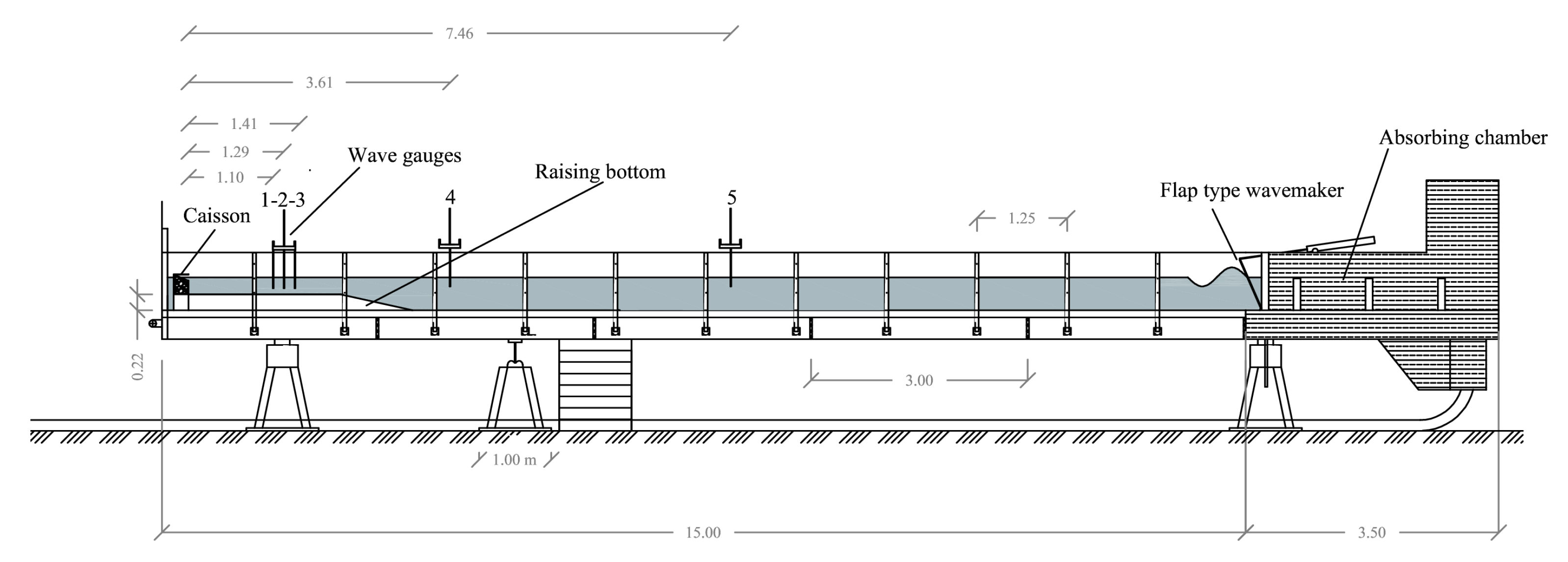
The flume is 18.5 m long, with a rectangular cross section of 0.4 m × 0.8 m; it has a flat stainless steel bed and glass walls made with 1.25 m × 0.8 m panels mounted on a steel frame. It is equipped at one end with a wave-maker capable of generating both regular and random waves (see Figure 2).
The opposite end is closed with a PVC bulkhead. The wave-maker is flap type and it oscillates around an initial position. The flap is operated by a pneumatic system and electronically controlled by the Jonswap Wave Generator Software. In the case of regular wave generation, the software allows the following data to be managed: sampling frequency, offset, frequency, and amplitude of the wave-maker oscillation. Detailed information of the wave flume can be found in Faraci [25] and Faraci et al. [26].
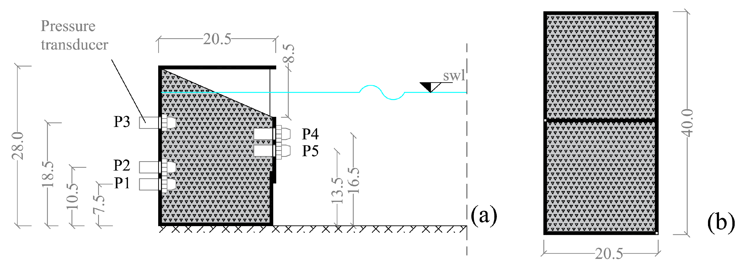
At the end of the channel, opposite to the wave-maker, a scaled model of a combined caisson with a 1:40 geometrical scale ratio is located (see Figure 3). The caisson model has dimensions 40 cm × 20.5 cm × 28 cm and is made of steel. Inside there is a separation wall that creates a double chamber in the cross section.
On the front face, the caisson presents a vertical wall that can be raised or lowered in order to adjust the size of the front opening; in the present study this opening was kept fixed and equal to 8.5 cm, in accordance with the findings of Faraci et al. [3].
The top cover has 8 holes with a diameter of 2 cm that act as vents.
The caisson is filled with gravel, to simulate the presence of large rock or concrete blocks. This filling was arranged in order to create a sloping surface (1:2.3) in correspondence with the opening of the caisson, that goes from the head of the front wall to the top of the rear wall, as shown in Figure 3. The rubble mound elements were modeled by means of marble pebbles whose average size is approximately 3 cm and porosity is 0.30.
The elevation of the free surface was measured by using five resistive wave gauges located along the flume. Three of them were placed at a relatively short distance from the caisson (≈1 wavelength) in order to evaluate the reflection coefficient, while the remaining 2 allowed the wave height far from the caisson to be monitored. Specifically, with respect to the front wall of the caisson, the probes were arranged as follows: probe 1 was placed at 1.10 m, probe 2 was placed at 1.29 m, probe 3 at 1.41 m, probe 4 at 3.61 m, and finally probe 5 at 7.46 m. The estimation of the amplitude of the incident and reflected waves was carried out by using the method proposed by [27].
Pressure measurement was carried out by means of the ATM.1ST/N transducers produced by STS (Sensor Technik Sirnach). In order to carry out the pressure measurements on the caisson, 3 pressure transducers were located inside it at the inner wall and two at the front wall. The elevation of the transducers were set equal to 7.5 cm, 10 cm, and 18 cm from the bottom at the rear wall; 13.5 cm and 16.5 cm from the bottom at the front wall. These sensors were mounted through holes suitably made on the walls as shown in Figure 3.
For all the tests, the data acquisition frequency was set equal to 100 Hz.
Table 1 shows the range of the wave characteristics estimated close to the model. The water depth was set equal to 0.235 m for all tests.
3. Numerical Model
The finite-volume based open source software OpenFOAM® was used for the CFD simulation. Such software, developed by OpenCFD Ltd since 2004, has a large user base across most engineering and science areas. In particular, it is widely used to simulate a great number of physical processes in coastal engineering [28,29,30,31]. Generally, Reynolds-Averaged Navier–Stokes (RANS) equations are used which represent the continuum characteristics of the fluid both in space and time.
As regard the solver for two-phase flow within porous media, the approach developed for the first time by the Environmental Hydraulics Institute IHCantabria and implemented in the toolbox olaflow was used in this study [8]. Such an approach is based on the Volume-average Reynolds-averaged Navier–Stokes (VARANS) equations [9] using the version proposed by del Jesus et al. [10]. In particular, the equations are [14]
where and indicate the components of the Darcy velocity , n is the porosity, is the density, p is the pressure, g is the acceleration of gravity, is the kinematic viscosity, and is the VOF indicator function. The term indicates the intrinsic velocity related to the portion of fluid within the gaps of the porous media. The last three terms of Equation (5) were included to take into account the resistance force due to the presence of the porous media (see also Equation (1)). In particular, such terms were added as closure terms to account for phenomena that cannot be solved when the volume-average method is used (i.e., frictional forces, pressure force, and added mass).
In order to align the momentum equation with the one implemented in OpenFOAM®, some adjustments of Equation (5) were proposed [14]:
When the porosity is equal to 1, it can be noted that Equation (7) can be applied outside porous media. Furthermore, the VARANS equations are identical to the classic RANS equations.
The pressure-velocity equations are solved by a two step PIMPLE method and the VOF function advection-diffusion equation is solved with the MULES method (multi-dimensional limiter for explicit solution). The PIMPLE method is derived from PISO (Pressure Implicit with Splitting of Operators) and SIMPLE (Semi-Implicit Method for Pressure-Linked Equations) algorithms. Among the several turbulence models offered in OpenFOAM®, the model SST- was used in the present study. Such a model has the advantage to combine the and turbulence models. The model is used in the boundary layer’s inner region, while the model is used in the free shear flow. Indeed, this allows a good performance of the numerical model also near the walls, within the boundary layer region [10,32]. In the present study, such a model allows the proper simulation of turbulence effects both during the interaction of the waves and the frontal wall and when the airflow penetrates through the holes of the top cover.
The toolbox olaflow offers a set of boundary conditions for generating and absorbing waves at the boundaries, with the advantage that a damping zone is not required, resulting in significant computational savings. The wave absorption of the numerical model is achieved by imposing at the inlet the expected velocity profile by means of the shallow water theory [32]. In the present study, first-order Stokes waves were imposed at the inlet. At the same boundary, the absorbing wave tool was activated to reduce the disturbance of reflected waves that reach the inlet.
3.1. Computational Domain and Boundary Conditions
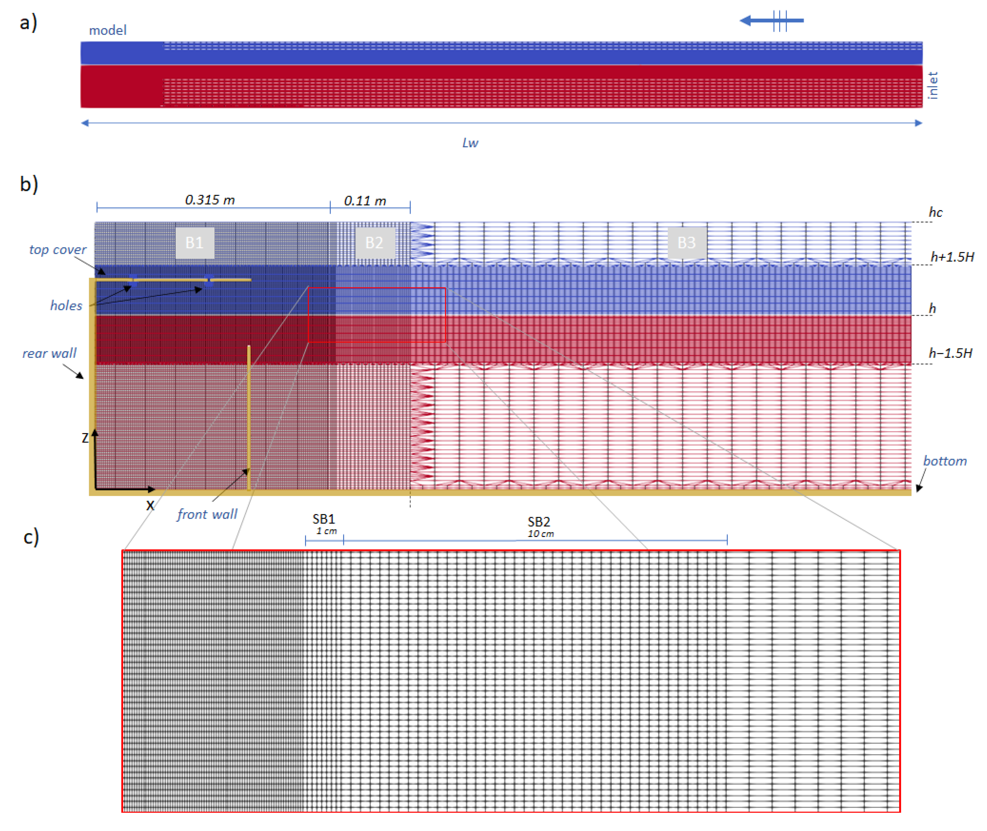
The computational domain is a numerical reproduction of the experimental caisson model. A two-dimensional simulation was used to study the behaviour of the anti-reflection structure. The reference system was set with the origin in the left bottom corner of the caisson, with x axis pointing against the wave propagation direction and z pointing upwards (see Figure 4).
The computational domain was discretized using the OpenFOAM® mesh generation tools: blockMesh and snappyHexMesh.
In order to reproduce adequately the hydrodynamics processes close to the composite caisson, the grid resolution gradually increases from the flume inlet to the model (see Figure 4). The cell number was defined according to specific guidelines and previous similar research works. In particular, the grid resolution of the zone where the water level fluctuation is expected was defined according to ITTC Guidelines [33]. The grid size at the composite caisson was defined in accordance to the studies of Vanneste and Troch [34], Elhanafi et al. [35], López et al. [36], and Cavallaro et al. [37].
In the zone where the water level fluctuation is expected, the grid size was imposed equal to /20 in the z-direction and equal to L/80 in the x-direction. was set equal to and the wavelength L was estimated through the dispersion relation using the wave period T and the water depth h.
The mesh generation was divided into a two-step process. In the first, a background mesh (or primitive mesh) of hexahedral cells that fill the entire wave flume using the OpenFOAM®’s tool blockMesh was generated. Then, using the tool snappyHexMesh, each cell was split according to the refinement level defined by the user. For example, fixing a refinement level of 1, which means the refinement factor is equal to , a cell of the background mesh will be cut in two along in each direction (creating 4 sub-cells for a 2D mesh). Such a refinement level can assume different values within the computational domain.
To generate the primitive mesh the domain was divided in three blocks: one placed in correspondence to the caisson model (), one relative to the opposite part of the channel (), and one of transition ().
The first block is 0.315 m long, that is * (1 + 0.5) where indicates the longitudinal length of the caisson. The size of the cell in x-direction was set equal to 0.005 m and the number of cells is 63.
The transition block is composed by two sub-blocks. The length of first sub-block (), close to block , is equal to 0.01 m while the length of the second sub-block () is equal to 0.10 m. In the primitive mesh, the sub-blocks and were composed by one and five cells respectively.
For the block , the number of the cells in the x-direction was defined by means the following relationship:
where function ⌈ provides the least integer greater than or equal to the argument of the function, is the length of the wave flume (estimated as ). The factor was applied to achieve the desired number of cells for the zone after the cell split carried out by the tool snappyHexMesh. For the present numerical simulation, a value of 3 was adopted.
In the z-direction, the computational domain is 0.36 m long and the number of cells in the primitive mesh was set equal to 30.
The generation of the final mesh was carried out by means of the function snappyHexMesh applied on the primitive mesh. The refinement factors shown in Table 2 were used. A refinement factor equal to 4 for the two holes placed at the top cover was set.
For the computational domain, proper boundary conditions were specified at domain boundaries (inlet, atmosphere) and physical boundaries (caisson walls, bottom). At the bottom and the walls of the composite caisson the no-slip boundary condition was imposed. For the atmosphere boundary, a fixed total pressure condition was used. Several regular waves were generated at the inlet, characterized by a wave height and a frequency in the range 0.01–0.06 m and 0.6–1.8 Hz (see Table 1), respectively. All cases simulated were generated using the first-order form of Stokes theory. Such a set of waves was simulated for both processes of validation and calibration.
3.2. Benchmark Test
To validate the setup of the numerical model (cell size, mesh refinement, turbulence model, boundary conditions, etc.), some experiments were carried out without the internal rubble mound of the composite caisson. This type of test allows any effects due to the porous media to be removed.
The experimental variables used in the validation process are the reflection coefficient and the wave pressure measured at the internal wall of the caisson at three different elevations. Such quantities represent the most important factors influencing the composite caisson design phase.
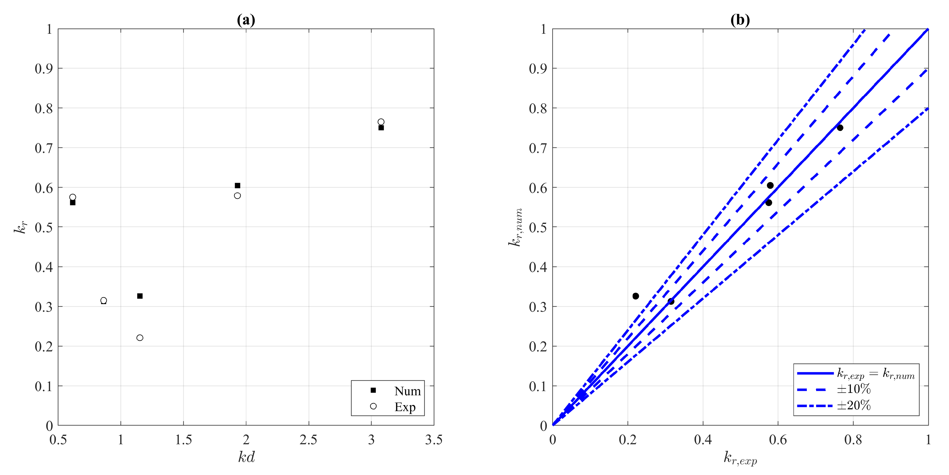
Figure 5 shows the comparison between the reflection coefficient () measured within the experimental campaign and that estimated by the numerical model. In general, the experimental and numerical data show the same trend. As regard the experimental data, the minimum value is detected for equal to 1.15, while according to the numerical model the minimum value occurs for equal to 0.86. However, the numerical reflection coefficient for = 0.86 ( = 0.32) and the one obtained for = 1.15 ( = 0.33) are pretty similar.
For = 1.15, the evaluated by the numerical model is higher than the experimental value, with an absolute difference approximately of 0.1 and a relative difference approximately of 60%. Such a difference presumably could be related to a not proper simulation of the energy dissipated by wave breaking that occurs close to the front wall.
For most of the simulated cases, the relative difference between the observed data and those estimated by the numerical model is very low. Data approximately show the same relative difference obtained in other numerical studies [38,39]. As can be seen from Figure 5, such difference in most cases is less than 10% (typical limit used in previous studies [36,39,40]).
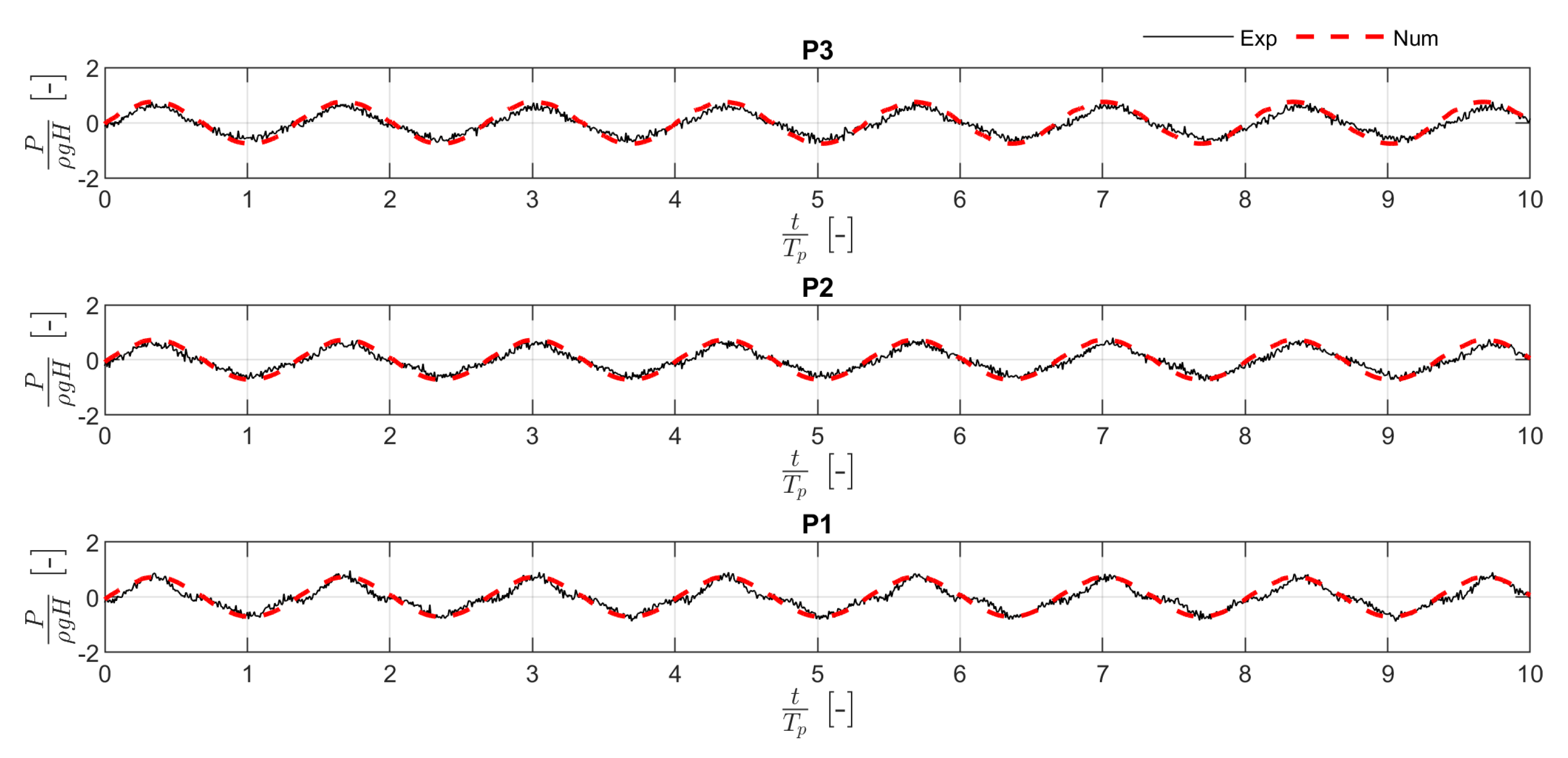
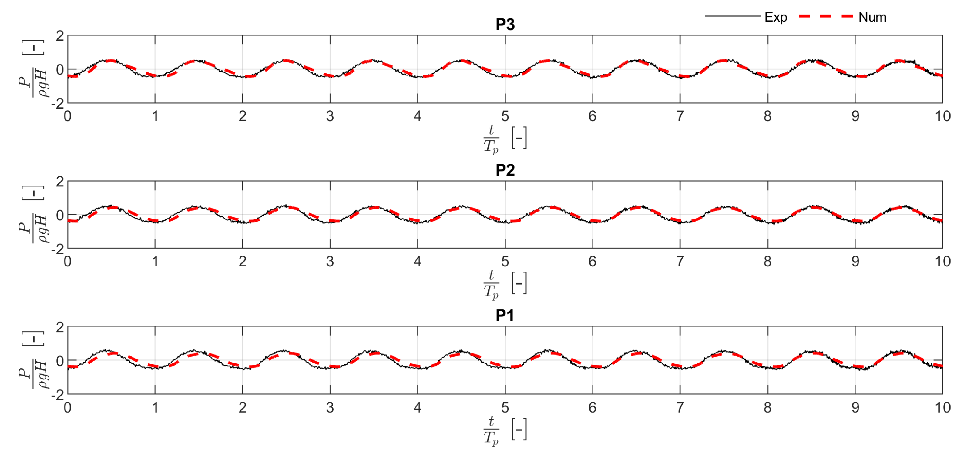
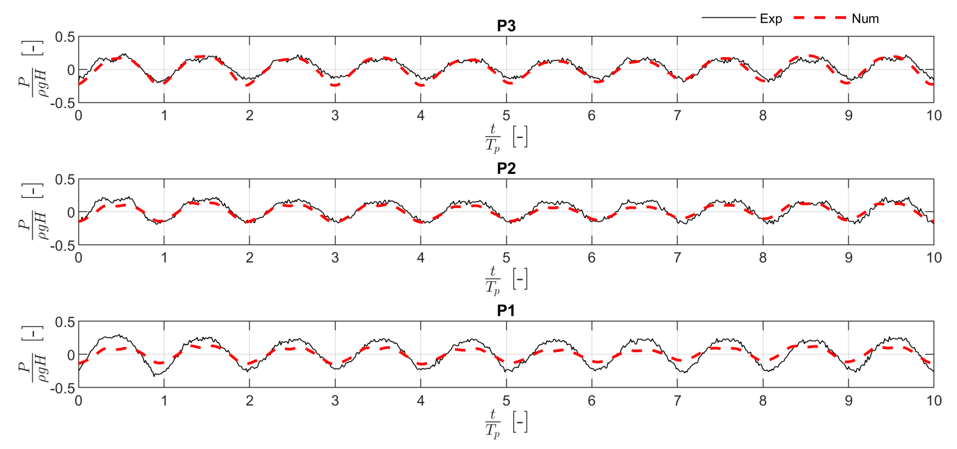
To test the ability of the numerical model in reproducing the pressure distribution in the space and time, Figure 6, Figure 7 and Figure 8 show the comparison between the time histories of the wave pressure at the rear wall of the caisson measured during the experimental campaign and those estimated by the numerical model at the same positions of the three transducers. The red dotted line in the figures denotes the numerical results. The pressure was made dimensionless through the hydrostatic pressure due to wave height (, where is the water density and g is the gravity acceleration). The horizontal axis represents the dimensionless time obtained from the ratio between the time and the wave period.
Generally, the numerical model well reproduces the signal obtained in the experimental campaign. In particular, the model provides an adequate approximation of the signal form and its amplitude. However, an overestimation of the pressure estimated for the wave with = 0.62 is detected. For a quantitative analysis, the comparison between the experimental and the numerical data was extended to the wave loading at the rear wall. In particular, the wave force () was estimated by integrating the pressure signals in the portion between 0.075 and 0.185 m from the bottom, which is the portion of the wall where the pressure transducers in the experimental campaign were placed (the length of such portion is indicated with ). To verify the reliability of the numerical model under both the wave crests and troughs, such a comparison was carried out on the basis the maximum () and the minimum () wave loading.
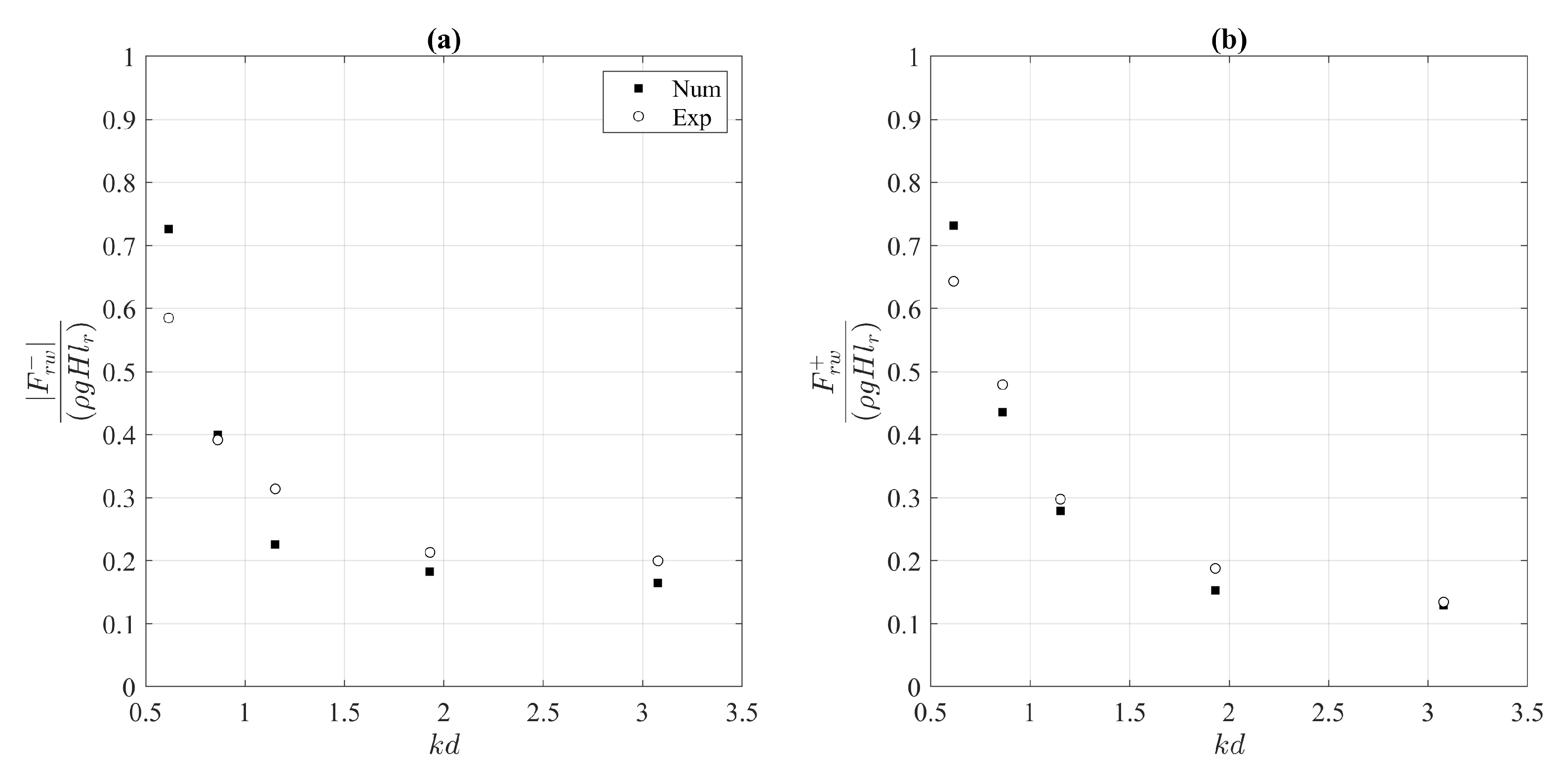
Figure 9 shows the comparison between the wave loading measured in the experimental campaign on the rear wall of the caisson and that estimated by the numerical model.
As can be seen from Figure 9, the numerical model well reproduces the experimental quantities even if an overestimation of the numerical model for low values of is observed.
The performance of the numerical model was measured by the following parameters: the root mean square error (rmse); the scatter index (si) and the slope. Such parameters are defined by the following relationship:
where and indicate the wave pressure estimated in the experimental campaign and by means the numerical model, respectively. According to such relationships, the perfect match between the experimental and numerical data is achieved when and are equal to zero and is equal to 1.
Table 3 shows the values of the performance parameters evaluated both for the reflection coefficient and the maximum and minimum wave loading at the rear wall.
Regarding the , the differences between the experimental and the numerical data are relatively small. The higher value of observed for the wave loading is mainly affected by the overestimated result observed for equal to 0.62. Regarding the values, they can be considered satisfactory for all three variables as they are close to 1. Based on these results, the setup of the numerical model for the study of the composite caisson can be assumed to be reliable.
4. Calibration of the Porous Media Parameters
The calibration of the closure terms in the VARANS equations (linear, nonlinear, and transient components) was carried out considering several values of and (see Equations (2) and (3)). Following previous studies, c was set equal to 0.34 [10,14,20].
and were defined according to other similar studies. In particular, the values adopted by Jensen et al. [18], Van Gent [20], Liu et al. [21], and Wu and Hsiao [22] were used as references. The following configurations were considered:
- Configuration 1 (C1): = 0.0 and = 0.0;
- Configuration 2 (C2): = 200 and = 1.1;
- Configuration 3 (C3): = 1000 and = 1.1;
- Configuration 4 (C4): = 200 and = 2.0;
- Configuration 5 (C5): = 1000 and = 2.0.
Configurations C2 and C3 allowed the effect of the coefficient related to the linear term to be evaluated; while C4 and C5, together with the previous configuration, allowed the effect of the parameter related to the nonlinear term to be tuned. Furthermore, an additional configuration (C1) was investigated where the three coefficients were set equal to zero. The latter was analyzed to quantify the response of the numerical model when the closure terms are not considered and only the effects due to the porosity (n) are present. Indeed, when the three coefficients are set to zero, the momentum equation (Equation (7)) takes into account only the rubble mound porosity.
Each configuration was tested considering the same waves of the validation cases (i.e., the cases in the absence of the porous media). On the complex, 25 sea states were simulated. The duration of each simulation was set equal to 100 s and the reflection coefficient and the wave loading both in the front wall and rear wall were estimated. It is important pointing out that the force was evaluated by integrating the pressure in the portion of the wall where the pressure probes are located, as above mentioned (the length of such portion is indicated with and at the rear wall and the front wall respectively).
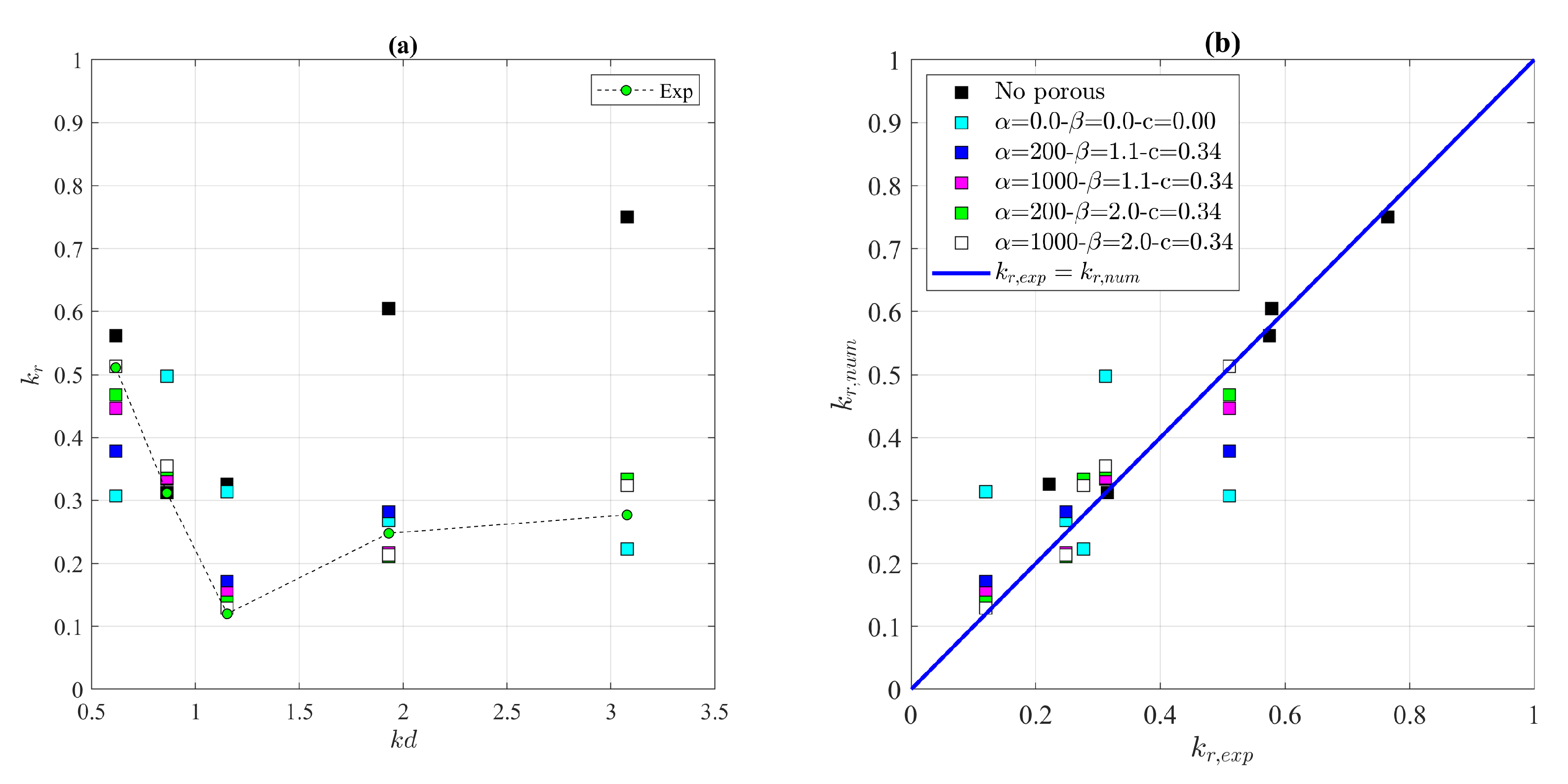
Figure 10 shows the comparison between the reflection coefficient estimated by the numerical model and by the experimental one.
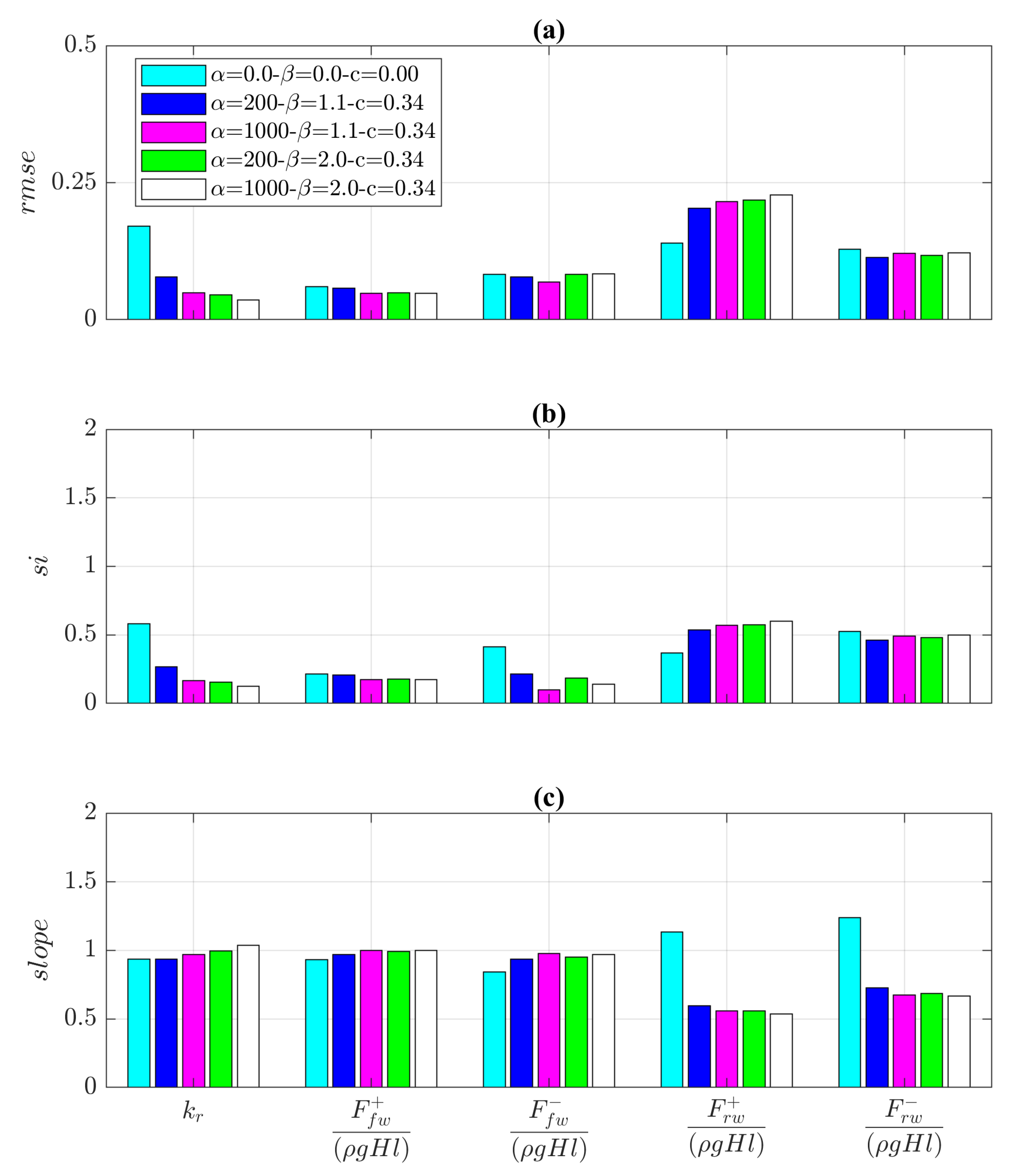
This comparison reveals the following aspects. For , the reflection coefficient observed in the experimental campaign for the tests without porous media presents a similar trend to that with porous media. For , the effect of the porous media is more significant. Regarding the calibration of the numerical model, the tuning of the coefficients determines greater variations in the cases with . For these wave conditions, the correspondence between observed and simulated data is more accurate as and are equal to 1000 and 2.0, respectively. In the case of null values of the coefficients , , and c, there are significant differences between the numerical model and the experimental data. Therefore, the configuration that guarantees the best performance is the one characterized by the following values of the coefficients: = 1000, = 2.0, and c = 0.34. For such a configuration, the performance parameters are = 0.04, = 0.12, and = 1.04; as a reference, for the configuration C1 (all coefficients are set equal to zero), the performance parameters are = 0.17, = 0.58, and = 0.94.
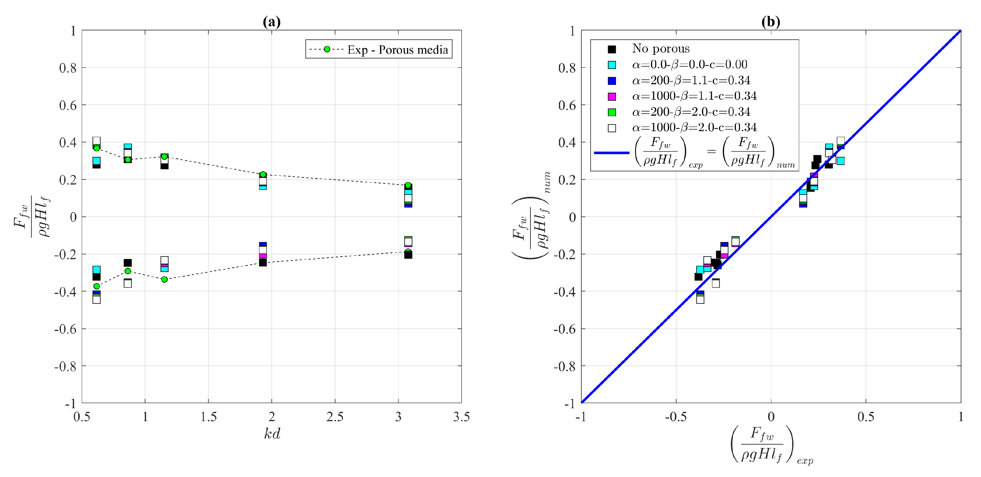
Figure 11 shows a comparison of the wave loading at the front wall estimated by the numerical model and those observed in the laboratory tests. The comparison between the experimental and the numerical data was extended to the wave loading at the front wall under both the wave crests () and troughs ().
The numerical model estimates the values detected in the experimental campaign with sufficient reliability. Almost the same values of the performance parameters are found for the various configurations analyzed. However, the best performance was estimated for the configurations C3, C4, and C5. For such configurations, the average performance parameters related to the maximum force are = 0.05, = 0.17, and = 1.00; while, for the configuration C1 (all coefficients are set equal to zero), the performance parameters are = 0.06, = 0.22, and = 0.93. As regards the minimum force, for the three configurations (C3, C4, and C5) the average performance parameters are = 0.08, = 0.14, and = 0.96; for the configuration C1 are = 0.08, = 0.41, and = 0.84.
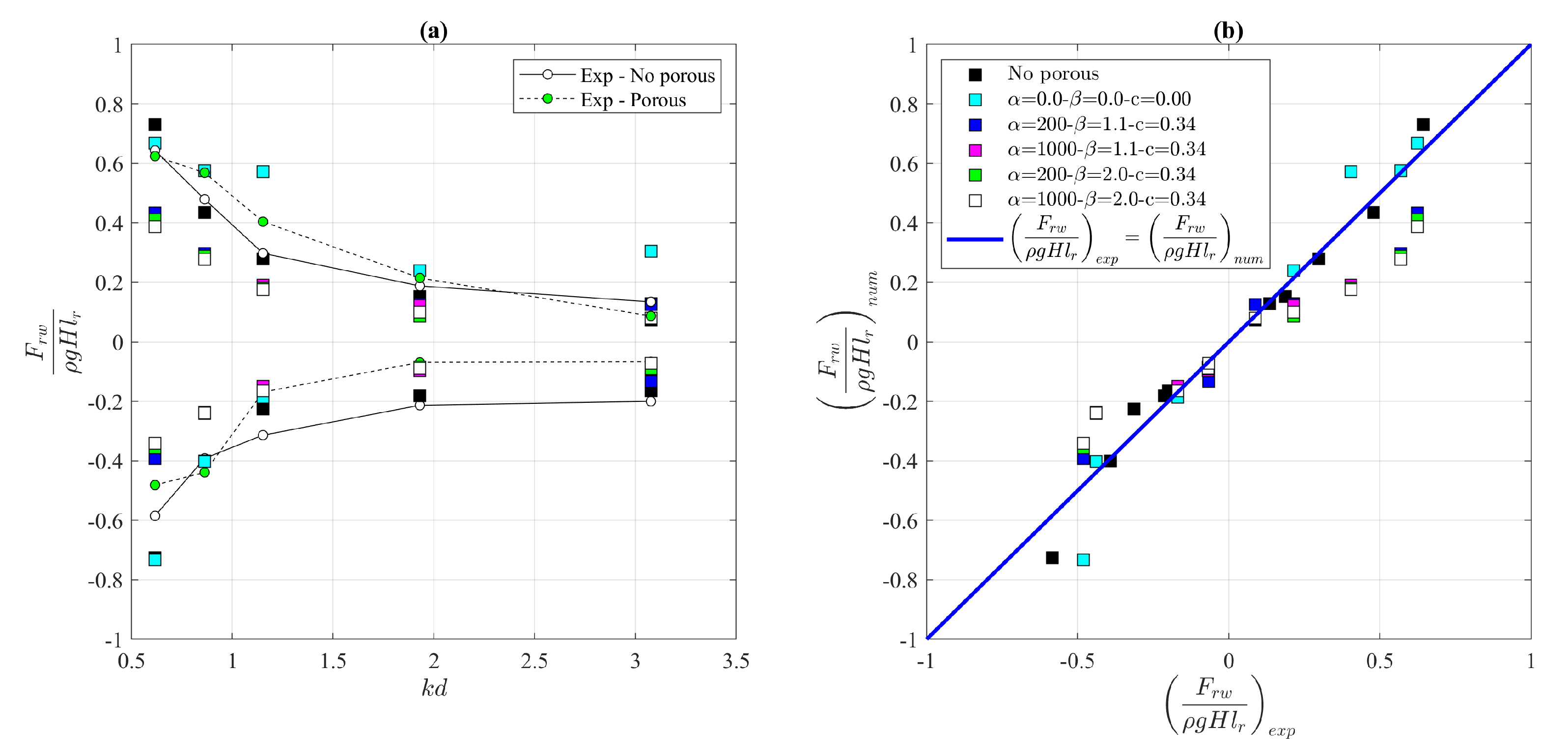
As can be seen from Figure 12, the maximum pressure measured in the experimental campaign is greater than in the configuration without the porous media. This behavior is determined by the hydrodynamics processes that occurred when the wave interacts with the structure and, in particular, with the rubble mound. The porous zone causes the rise of the wave up to the top cover of the composite caisson, causing a maximum pressure that is greater than that observed in the case without the internal rubble mound. This aspect is more significant for longer waves characterized by between 0.62 and 1.15. As regards the negative pressure, the presence of the porous zone determines the attenuation of wave pressure.
Compared to the previous cases, the force on the rear wall is the one that is most affected by the adopted numerical methodology and, in particular, by the values of the coefficients and .
The presence of the porous element determines an underestimation of the forces for configurations C2, C3 C4 and C5 ( and greater than zero). Such behaviour is due to confined motion which determines extremely low velocity of the fluid into the porous media. The use of the coefficients and greater than zero involves an increase in the drag force which is not in conformity with that detected in the experimental campaign.
For the configurations C2, C3, C4, and C5 ( and greater than zero), the average performance parameters related to the maximum force are = 0.22, = 0.57, and = 0.56; while, for the configuration C1 (all coefficients set equal to zero), the performance parameters are = 0.14, = 0.37, and = 1.13. Regards the minimum force, the performance parameters are: for the configurations C2-C5 with and greater than zero, = 0.12, = 0.48, and = 0.69; for the configuration C1, = 0.13, = 0.53, and = 1.24.
A synthetic overview of the performances estimated for all configurations is shown in Figure 13. The figure shows the performances of the configurations tested in the present study expressed through , , and .
5. Conclusions
The purpose of this work is the calibration of a numerical model based on VARANS equations for simulating the interaction of waves and a composite caisson with an internal rubble mound to dissipate incident sea wave energy. To take into account the drag forces due to porous media which cannot be estimated when the volume-average method is used, the calibration of two coefficients ( and ) is required.
Following other authors, in the present study several configurations of and were analyzed to find which better fit the data observed within the experimental campaign carried out at the hydraulic laboratory of the University of Messina.
The analyses were carried out considering as reference quantities the reflection coefficient and the force that waves exert on a portion of vertical walls of the composite caisson. The results showed that the numerical model can adequately reproduce the reflection coefficient and the forces on the front wall. In particular, the best results are obtained as and are equal to 1000 and 2.0, respectively.
Regarding the wave loading on the inner wall, some limits of the numerical model arise. In particular, the greatest differences between the numerical and experimental data are found for the maximum force.
In general, it is observed that for any value of and a drag force is generated which attenuates the action of the wave motion much more than in laboratory tests. Indeed, extremely low speeds are expected within the porous body. Nevertheless, the use of the coefficients and involves a fictitious drag force, which is much greater than that observed in reality. Accordingly, forces are best simulated when all the coefficients are set to zero.
In this case, a good agreement with laboratory data was achieved, although an overestimation of wave loading was observed in some simulated cases.
In the light of these results, it can be concluded that:
- the behaviour of the composite caisson can be adequately simulated using VARANS equations;
- the reflection coefficient and the force in the front wall are well reproduced when a value of = 1000 and = 2.0 are used;
- the force at the rear wall is underestimated when the terms related to drag force are considered (i.e., > 0 and/or > 0); and
- if the drag forces due to the rubble mound is not considered, a precautionary estimate of the forces at the rear wall is obtained.
Future research activities will focus on a comparative analysis between the simulation conducted through VARANS equation and those carried out by conventional RANS equation applied to the effective porous media structure.
Author Contributions
Conceptualization, C.I., L.C., E.F. and C.F.; Formal analysis, C.I. and L.C.; Investigation, C.I. and L.C.; Methodology, C.I.; Supervision, E.F. and C.F.; Visualization, C.I. and L.C.; Writing—original draft, C.I. and L.C.; Writing—review and editing, C.I., L.C., E.F. and C.F. All authors have read and agreed to the published version of the manuscript.
Funding
‘This work has been partly supported by the project TETI-TEcnologie innovative per il controllo, il monitoraggio e la sicurezza in mare (code ARS01_00333) and by the project ISYPORT-Integrated SYstem for navigation risk mitigation in PORTs (code ARS01_01202).
Institutional Review Board Statement
Not applicable.
Informed Consent Statement
Not applicable.
Data Availability Statement
Not applicable.
Conflicts of Interest
The authors declare no conflict of interest.
References
- Zanuttigh, B.; van der Meer, J.W. Wave reflection from coastal structures in design conditions. Coast. Eng. 2008, 55, 771–779. [Google Scholar] [CrossRef]
- Altomare, C.; Gironella, X.; Sanchez-Arcilla, A.; Sospedra, J. Wave reflection on dissipative quay walls: An experimental study. In Proceedings of the International Conference of the Application of Physical Modeling to Port and Coastal Protection, Ghent, Belgium, 17–20 September 2012; pp. 779–786. [Google Scholar]
- Faraci, C.; Scandura, P.; Foti, E. Reflection of sea waves by combined caissons. J. Waterw. Port Coast. Ocean Eng. 2015, 141, 04014036. [Google Scholar] [CrossRef]
- Altomare, C.; Gironella, X. An experimental study on scale effects in wave reflection of low-reflective quay walls with internal rubble mound for regular and random waves. Coast. Eng. 2014, 90, 51–63. [Google Scholar] [CrossRef]
- Faraci, C.; Cammaroto, B.; Cavallaro, L.; Foti, E. Wave reflection generated by caissons with internal rubble mound of variable slope. In Proceedings of the 33rd International Conference on Coastal Engineering, Santander, Spain, 1–6 July 2012; Volume 16. [Google Scholar]
- Liu, Y.; Faraci, C. Analysis of orthogonal wave reflection by a caisson with open front chamber filled with sloping rubble mound. Coast. Eng. 2014, 91, 151–163. [Google Scholar] [CrossRef]
- Faraci, C.; Liu, Y. Analysis of wave forces acting on combined caissons with inner slope rubble mound. Coast. Eng. 2014, 34. [Google Scholar] [CrossRef] [Green Version]
- Higuera, P. olaFlow: CFD for Waves [Software]. 2017. Available online: https://doi.org/10.5281/zenodo.1297013 (accessed on 7 October 2021).
- Hsu, T.J.; Sakakiyama, T.; Liu, P.L.F. A numerical model for wave motions and turbulence flows in front of a composite breakwater. Coast. Eng. 2002, 46, 25–50. [Google Scholar] [CrossRef]
- del Jesus, M.; Lara, J.L.; Losada, I.J. Three-dimensional interaction of waves and porous coastal structures: Part I: Numerical model formulation. Coast. Eng. 2012, 64, 57–72. [Google Scholar] [CrossRef]
- Darcy, H. Les Fontaines Publiques de la ville de Dijon: Exposition et Application...; Victor Dalmont: Paris, France, 1856. [Google Scholar]
- Forchheimer, P. Wasserbewegung durch boden. Z. Ver. Deutsch. Ing. 1901, 45, 1782–1788. [Google Scholar]
- Polubarinova-Koch, P.I. Theory of Ground Water Movement; Princeton University Press: Princeton, NJ, USA, 2015. [Google Scholar]
- Higuera, P.; Lara, J.L.; Losada, I.J. Three-dimensional interaction of waves and porous coastal structures using OpenFOAM®. Part I: Formulation and validation. Coast. Eng. 2014, 83, 243–258. [Google Scholar] [CrossRef]
- Feichtner, A.; Mackay, E.; Tabor, G.; Thies, P.R.; Johanning, L.; Ning, D. Using a porous-media approach for CFD modelling of wave interaction with thin perforated structures. J. Ocean Eng. Mar. Energy 2021, 7, 1–23. [Google Scholar] [CrossRef]
- Engelund, F. On the Laminar and Turbulent Flows of Ground Water through Homogeneous Sand; Akademiet for de Tekniske Videnskaber: Copenhagen, Denmark, 1953. [Google Scholar]
- Van Gent, M.R.A. Wave interaction with permeable coastal structures. Int. J. Rock Mechan. Min. Sci. Geomechan. Abstracts 1996, 6, 277A. [Google Scholar]
- Jensen, B.; Jacobsen, N.G.; Christensen, E.D. Investigations on the porous media equations and resistance coefficients for coastal structures. Coast. Eng. 2014, 84, 56–72. [Google Scholar] [CrossRef]
- Losada, I.J.; Lara, J.L.; del Jesus, M. Modeling the interaction of water waves with porous coastal structures. J. Waterw. Port Coast. Ocean Eng. 2016, 142, 03116003. [Google Scholar] [CrossRef]
- Van Gent, M. Wave Interaction with Permeable Coastal Structures. Ph.D. Thesis, Delft University of Technology, Delft, The Netherlands, 1995. [Google Scholar]
- Liu, P.L.F.; Lin, P.; Chang, K.A.; Sakakiyama, T. Numerical modeling of wave interaction with porous structures. J. Waterw. Port Coast. Ocean Eng. 1999, 125, 322–330. [Google Scholar] [CrossRef]
- Wu, Y.T.; Hsiao, S.C. Propagation of solitary waves over a submerged permeable breakwater. Coast. Eng. 2013, 81, 1–18. [Google Scholar] [CrossRef]
- Lara, J.L.; Losada, I.J.; Maza, M.; Guanche, R. Breaking solitary wave evolution over a porous underwater step. Coast. Eng. 2011, 58, 837–850. [Google Scholar] [CrossRef]
- Vieira, F.; Taveira-Pinto, F.; Rosa-Santos, P. Novel time-efficient approach to calibrate VARANS-VOF models for simulation of wave interaction with porous structures using Artificial Neural Networks. Ocean Eng. 2021, 235, 109375. [Google Scholar] [CrossRef]
- Faraci, C. Experimental investigation of the hydro-morphodynamic performances of a geocontainer submerged reef. J. Waterw. Port Coast. Ocean Eng. 2018, 144, 04017045. [Google Scholar] [CrossRef]
- Faraci, C.; Scandura, P.; Petrotta, C.; Foti, E. Wave-induced oscillatory flow over a sloping rippled bed. Water 2019, 11, 1618. [Google Scholar] [CrossRef] [Green Version]
- Mansard, E.P.; Funke, E. The measurement of incident and reflected spectra using a least squares method. In Proceedings of the 17th International Conference on Coastal Engineering, Sydney, Australia, 23–28 March 1980; pp. 154–172. [Google Scholar]
- Higuera, P.; Lara, J.L.; Losada, I.J. Simulating coastal engineering processes with OpenFOAM®. Coast. Eng. 2013, 71, 119–134. [Google Scholar] [CrossRef]
- Higuera, P.; Lara, J.L.; Losada, I.J. Three-dimensional interaction of waves and porous coastal structures using OpenFOAM®. Part II: Application. Coast. Eng. 2014, 83, 259–270. [Google Scholar] [CrossRef]
- Devolder, B.; Rauwoens, P.; Troch, P. Application of a buoyancy-modified k-ω SST turbulence model to simulate wave run-up around a monopile subjected to regular waves using OpenFOAM®. Coast. Eng. 2017, 125, 81–94. [Google Scholar] [CrossRef] [Green Version]
- Di Paolo, B.; Lara, J.L.; Barajas, G.; Losada, Í.J. Waves and structure interaction using multi-domain couplings for Navier-Stokes solvers in OpenFOAM®. Part II: Validation and application to complex cases. Coast. Eng. 2021, 164, 103818. [Google Scholar] [CrossRef]
- Higuera, P.; Lara, J.L.; Losada, I.J. Realistic wave generation and active wave absorption for Navier–Stokes models: Application to OpenFOAM®. Coast. Eng. 2013, 71, 102–118. [Google Scholar] [CrossRef]
- ITTC. Practical guidelines for ship CFD applications. In Recommended Procedures and Guidelines; 2011; p. 18. Available online: https://ittc.info/media/1357/75-03-02-03.pdf (accessed on 7 October 2021).
- Vanneste, D.; Troch, P. 2D numerical simulation of large-scale physical model tests of wave interaction with a rubble-mound breakwater. Coast. Eng. 2015, 103, 22–41. [Google Scholar] [CrossRef]
- Elhanafi, A.; Macfarlane, G.; Fleming, A.; Leong, Z. Experimental and numerical measurements of wave forces on a 3D offshore stationary OWC wave energy converter. Ocean Eng. 2017, 144, 98–117. [Google Scholar] [CrossRef]
- López, I.; Rosa-Santos, P.; Moreira, C.; Taveira-Pinto, F. RANS-VOF modelling of the hydraulic performance of the LOWREB caisson. Coast. Eng. 2018, 140, 161–174. [Google Scholar] [CrossRef]
- Cavallaro, L.; Iuppa, C.; Musumeci, R.E.; Scandura, P.; Foti, E. Wave loads on a navigation lock sliding gate: Non-linear effects. Coast. Eng. Proc. 2020, 8. [Google Scholar] [CrossRef]
- Wang, D.X.; Dong, S.; Sun, J.W. Numerical modeling of the interactions between waves and a Jarlan-type caisson breakwater using OpenFOAM. Ocean Eng. 2019, 188, 106230. [Google Scholar] [CrossRef]
- Liu, X.; Liu, Y.; Lin, P.; Li, A.j. Numerical simulation of wave overtopping above perforated caisson breakwaters. Coast. Eng. 2021, 163, 103795. [Google Scholar] [CrossRef]
- Jacobsen, N.G.; van Gent, M.R.; Wolters, G. Numerical analysis of the interaction of irregular waves with two dimensional permeable coastal structures. Coast. Eng. 2015, 102, 13–29. [Google Scholar] [CrossRef]
Figure 1.
Cross section of a combined caisson.

Figure 2.
Cross section of the adopted wave flume belonging to Hydraulics Laboratory at the University of Messina (dimension in m).
Figure 2.
Cross section of the adopted wave flume belonging to Hydraulics Laboratory at the University of Messina (dimension in m).

Figure 3.
Cross section (a) and plan view (b) of the composite caisson (dimension in cm).

Figure 4.
Computational domain used for the numerical simulation of the composite caisson: (a) cross section of the entire domain; (b) detail of the grid close to the model; (c) detail of the grid in the transition zone. The symbols indicate , , and the name of the three blocks; and the name of the two sub-blocks; the height of the numerical flume; h the mean water level; and H the height of the incident regular waves.

Figure 5.
Reflection coefficient: (a) reflection coefficient measured in the experimental campaign and that estimate by the numerical model as a function of the parameter ; (b) comparison between the reflection coefficient measured in the experimental campaign and that estimated by the numerical model. The dashed lines represent the limits of 10% and 20% usually assumed in previous studies for this kind of comparison.

Figure 6.
Comparison between the pressure measured in the experimental campaign by the three transducers located on the rear wall and that estimated by the numerical model. The data refer to a wave with = 0.62.
Figure 6.
Comparison between the pressure measured in the experimental campaign by the three transducers located on the rear wall and that estimated by the numerical model. The data refer to a wave with = 0.62.

Figure 7.
Comparison between the pressure measured in the experimental campaign by the three transducers located on the rear wall and that estimated by the numerical model. The data refer to a wave with = 0.86.
Figure 7.
Comparison between the pressure measured in the experimental campaign by the three transducers located on the rear wall and that estimated by the numerical model. The data refer to a wave with = 0.86.

Figure 8.
Comparison between the pressure measured in the experimental campaign by the three transducers located on the rear wall and that estimated by the numerical model. The data refers to a wave with = 1.93.
Figure 8.
Comparison between the pressure measured in the experimental campaign by the three transducers located on the rear wall and that estimated by the numerical model. The data refers to a wave with = 1.93.

Figure 9.
Comparison between the wave loading measured in the experimental campaign on the rear wall of the caisson and that estimated by the numerical model. (a) and (b) indicate the minimum and maximum wave loading respectively.
Figure 9.
Comparison between the wave loading measured in the experimental campaign on the rear wall of the caisson and that estimated by the numerical model. (a) and (b) indicate the minimum and maximum wave loading respectively.

Figure 10.
Comparison between the reflection coefficient estimated from the experimental data and that estimated from the numerical model: (a) reflection coefficient as a of function ; (b) experimental data vs. numerical data.
Figure 10.
Comparison between the reflection coefficient estimated from the experimental data and that estimated from the numerical model: (a) reflection coefficient as a of function ; (b) experimental data vs. numerical data.

Figure 11.
Comparison between the wave loading at the front wall estimated from the experimental data and that estimated from the numerical model: (a) dimensionless wave loading as a function of ; (b) vs. .
Figure 11.
Comparison between the wave loading at the front wall estimated from the experimental data and that estimated from the numerical model: (a) dimensionless wave loading as a function of ; (b) vs. .

Figure 12.
Comparison between the wave loading at the rear wall estimated from the experimental data and that estimated from the numerical model: (a) as a function of ; (b) vs. .
Figure 12.
Comparison between the wave loading at the rear wall estimated from the experimental data and that estimated from the numerical model: (a) as a function of ; (b) vs. .

Figure 13.
Performance of the configurations tested expressed through (a), (b) and (c).


Table 1.
Wave characteristics close to the model (where the symbols indicate: H wave height, f wave frequency, T wave period, L wavelength, wave number, and d water depth). The wavelength was estimated through the dispersion relation.
Table 1.
Wave characteristics close to the model (where the symbols indicate: H wave height, f wave frequency, T wave period, L wavelength, wave number, and d water depth). The wavelength was estimated through the dispersion relation.
| N. | H [m] | f [Hz] | T [s] | L [m] | [−] |
|---|---|---|---|---|---|
| 1 | 0.01 | 0.60 | 1.67 | 2.40 | 0.62 |
| 2 | 0.03 | 0.80 | 1.25 | 1.71 | 0.86 |
| 3 | 0.06 | 1.00 | 1.00 | 1.28 | 1.15 |
| 4 | 0.05 | 1.40 | 0.71 | 0.76 | 1.93 |
| 5 | 0.02 | 1.80 | 0.56 | 0.48 | 3.08 |
Table 2.
Refinement factor used for as input for the OpenFOAM®’s function snappyHexMesh.
| Zone | Factor |
|---|---|
| and | 1 |
| and | 1 |
| and | 2 |
| and | 2 |
| and | 3 |
Table 3.
Performances parameters of the numerical model: the root mean square discrepancy between the two sets of data (rmse), the scatter index (si), and the slope.
Table 3.
Performances parameters of the numerical model: the root mean square discrepancy between the two sets of data (rmse), the scatter index (si), and the slope.
| Variables | rmes [−] | si [−] | slope [−] |
|---|---|---|---|
| 0.06 | 0.15 | 1.02 | |
| 0.08 | 0.25 | 1.07 | |
| 0.05 | 0.10 | 1.01 |
Publisher’s Note: MDPI stays neutral with regard to jurisdictional claims in published maps and institutional affiliations. |
© 2021 by the authors. Licensee MDPI, Basel, Switzerland. This article is an open access article distributed under the terms and conditions of the Creative Commons Attribution (CC BY) license (https://creativecommons.org/licenses/by/4.0/).
Share and Cite
MDPI and ACS Style
Iuppa, C.; Carlo, L.; Foti, E.; Faraci, C. Calibration of CFD Numerical Model for the Analysis of a Combined Caisson. Water 2021, 13, 2862. https://doi.org/10.3390/w13202862
AMA Style
Iuppa C, Carlo L, Foti E, Faraci C. Calibration of CFD Numerical Model for the Analysis of a Combined Caisson. Water. 2021; 13(20):2862. https://doi.org/10.3390/w13202862
Chicago/Turabian StyleIuppa, Claudio, Lilia Carlo, Enrico Foti, and Carla Faraci. 2021. "Calibration of CFD Numerical Model for the Analysis of a Combined Caisson" Water 13, no. 20: 2862. https://doi.org/10.3390/w13202862
Note that from the first issue of 2016, this journal uses article numbers instead of page numbers. See further details here.