
A Comparison of BPNN, GMDH, and ARIMA for Monthly Rainfall Forecasting Based on Wavelet Packet Decomposition


1
Henan Key Laboratory of Water Resources Conservation and Intensive Utilization in the Yellow River Basin, College of Water Resources, North China University of Water Resources and Electric Power, Zhengzhou 450046, China
2
Department of Civil and Environmental Engineering, The Hong Kong Polytechnic University, Hung Hom, Kowloon, Hong Kong, China
3
China Institute of Water Resources and Hydropower Research, Beijing 100081, China
*
Author to whom correspondence should be addressed.
Water 2021, 13(20), 2871; https://doi.org/10.3390/w13202871
Submission received: 6 September 2021
/
Revised: 7 October 2021
/
Accepted: 12 October 2021
/
Published: 14 October 2021
(This article belongs to the Special Issue Climate Changes and Hydrological Processes)
Abstract
:Accurate rainfall forecasting in watersheds is of indispensable importance for predicting streamflow and flash floods. This paper investigates the accuracy of several forecasting technologies based on Wavelet Packet Decomposition (WPD) in monthly rainfall forecasting. First, WPD decomposes the observed monthly rainfall data into several subcomponents. Then, three data-based models, namely Back-propagation Neural Network (BPNN) model, group method of data handing (GMDH) model, and autoregressive integrated moving average (ARIMA) model, are utilized to complete the prediction of the decomposed monthly rainfall series, respectively. Finally, the ensemble prediction result of the model is formulated by summing the outputs of all submodules. Meanwhile, these six models are employed for benchmark comparison to study the prediction performance of these conjunction methods, which are BPNN, WPD-BPNN, GMDH, WPD-GMDH, ARIMA, and WPD-ARIMA models. The paper takes monthly data from Luoning and Zuoyu stations in Luoyang city of China as the case study. The performance of these conjunction methods is tested by four quantitative indexes. Results show that WPD can efficiently improve the forecasting accuracy and the proposed WPD-BPNN model can achieve better prediction results. It is concluded that the hybrid forecast model is a very efficient tool to improve the accuracy of mid- and long-term rainfall forecasting.
1. Introduction
Hydrological time series forecasting is essential for a variety of real-world managements or operation of water resources systems [1,2]. Precipitation is affected by many factors such as atmospheric circulation, topography, climate change, and human activities. The improvement of precipitation prediction has received a lot of attention across the world and many models have been constructed to improve the hydrological process simulation and prediction accuracy [3,4,5].
These models can fall into two categories: knowledge-based models and data-based models [6]. Knowledge-based model is a numerical simulation technology that describes natural phenomena on the basis of an internal physical mechanism of the system [7]. However, the lack of multisource information and optimization complexity of computation parameters limit the generalization of physical-based models [8]. In contrast, data-based models can obtain satisfying results by using historical data without involving the physical load within hydrological time series [9,10]. Hence data-based models have received a lot of attention in the hydrological forecasting field. In this paper, we are devoted to verifying several data-based models for monthly rainfall time series forecasting. There are many data-based models, e.g., artificial neural networks (ANN) [11], genetic programming (GP) [12], support vector machines (SVM) [13], and adaptive neuro-fuzzy inference system (ANFIS) [14].
Box–Jenkins models [15], which are considered as the most comprehensive tool in all statistical methods of time series forecasting, include auto-regressive (AR), moving average (MA), autoregressive moving average (ARMA), ARIMA, and other models. ARIMA is a linear statistical model and normally used to simulate and forecast time series with temporal correlation [16,17]. With the advance of technology such as computers, communication, remote sensing, and geography information systems, the prediction ability of the ARIMA model has been greatly improved [18]. Rahman et al. [19] used Mann–Kendall, Spearman’s rho test, and the ARIMA model to analyze and predict rainfall trends in Bangladesh. Mishra et al. [20] compared seasonal ARIMA and ARIMA models for runoff forecasting accuracy in the River Brahmaputra Basin, and the results indicated that ARIMA could provide higher accuracy. Rizeei et al. [21] combined a soil conservation service–curve number (SCS-CN) model with an ARIMA and land transformation model to monitor the changes of surface runoff. Wang et al. [22] proposed a hybrid Empirical Mode Decomposition (EMD)/Ensemble Empirical Mode Decomposition (EEMD)-ARIMA model for long-term runoff forecasting.
ANN, a nonlinear data-based model, is extensively used for hydrological applications [23,24]. The major application of ANN can be summarized as streamflow forecasting [25,26], rainfall forecasting [27,28], groundwater problems [29,30], suspended sediment estimation [31], regional drought analysis and forecasting [32,33], etc. Among different kinds of ANN, BPNN is a multilayer feed forward ANN with unidirectional transmission, which has advantages of learning and extracting the features, memory association, parallel architecture, and independent learning and adaptive capabilities [34]. The BPNN model has been widely applied to precipitation prediction, study of rainfall prediction with meteorological parameters [35], estimation of regional surface soil moisture [36,37], etc. Consequently, we attempt to use BPNN for monthly rainfall forecasting as a nonlinear data-based model.
GMDH is a sub-model of ANN for complex system modeling [38]. The main principle is to construct an analytic function of the system by quadratic node transfer function. The coefficients of binomial transfer function are obtained by polynomial regression. GMDH has been successfully used in broad fields such as economics, engineering, science, medical diagnostics, control systems, signal processing, and water resources [39,40].
Although the performance of ANN is remarkable in dealing with linear problems, it cannot handle non-stationary and nonlinear problems that arise in rainfall data. Studies have shown that forecasting accuracy of models could be improved by appropriate data preprocessing techniques to eliminate noises in hydrological time series. In recent years, many scholars have performed a lot of work based on this idea to improve the prediction performance of models. Partal and Kişi [41] proposed a wavelet-neuro-fuzzy model, especially suitable for forecasting daily rainfall time series, which have zero rainfall in summer months. Wang, et al. [42] proposed the EEMD-ANN model to forecast medium- and long-term runoff time series. Yu, et al. [43] explored Fourier transform (FT) and support vector regression (SVR) for forecasting monthly reservoir inflow and compared them with EEMD-SVR and SSA-SVR models, and found that FT-SVR consumed more computational resources in parameter calibration. The least-squares wavelet analysis (LSWA) [2] has shown promising results in successful analysis of streamflow and climate time series. Feng, et al. [44] combined variational mode decomposition (VMD), SVM, and quantum-behaved particle swarm optimization (QPSO) to forecast monthly streamflow and achieved excellent prediction results.
Most common decomposition approaches perform well only when the input variables meet certain conditions. For example, EMD may suffer from mode mixing due to intermittent signal [45], and this effect is important to hydrological applications. The stationarity of time series has a great influence on the accuracy of position in the domain identified by FT method [46]. Nevertheless, hydrological time series are non-stationary, which means that statistical properties will fluctuate over time [47]. In recent years, researchers have paid great attention in WPD. The main idea of WPD method is using multiple filters to decompose the original signal into more linear sub-signals with different frequency characteristics, which can be regarded as an improved version of the wavelet decomposition (WD). In discrete wavelet transform (DWT), when performing next layer decomposition, only approximate coefficients obtained from the upper layer can pass through the filter [48]. However, when the WPD method performs the next level of decomposition, both the low-frequency sequence and high-frequency sequence can pass the filter [49], and the total number of coefficients is still the same without redundancy. Therefore, WPD can extract the features of the original signal more comprehensively, which not only provides a wide range of possibilities for signal analysis but also allows the best matching analysis of the signal. Meanwhile, compared with DWT, the decomposition structure of WPD provides more opportunities to improve computational efficiency [50]. Therefore, WPD is preferred in this paper in consideration of the complex nonlinearity and non-stationary characteristics of hydrologic time series.
The purpose of this paper is to investigate the accuracy of ARIMA, GMDH, and BPNN models based on WPD in monthly rainfall forecasting. Most former research often improve the accuracy of prediction models by optimizing model parameters using optimization algorithms, and the improvement effect of this method is often not obvious. In this paper, the data preprocessing method is adopted to improve the accuracy of forecasting models, which can attain more linear sub-series and significantly reduce the difficulty of prediction. Firstly, we use WPD to decompose original monthly rainfall series into a series of sub-series with different frequencies and spatiotemporal resolutions. Then, the subseries decomposed by WPD are used as input data of ARIMA, GMDH, and BPNN to train for prediction. Finally, the prediction results of each hybrid model are obtained by linearly accumulating the outputs of each submodule.
2. Materials and Methods
2.1. Study Region
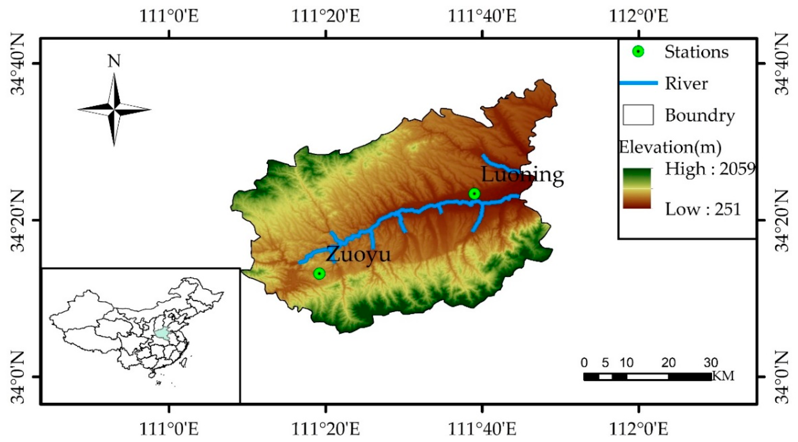
Two hydrological stations located in Yiluo River Basin on the south bank of the middle stream of Yellow River are considered as the case study. Yiluo River is an important first-level tributary of Yellow River and one of the main sources of floods in the lower reaches of Yellow River, with a drainage area of 18,881 km2. The mainstream Luo River is 446.9 km long, and the tributary Yi River is 264.8 km long. Luoning and Zuoyu Stations are located in the middle stream of Luo River and the middle and upper stream of Yi River, respectively. The average annual rainfall of the two stations are 635.2 mm and 834.3 mm, respectively. The inter-seasonal fluctuations of rainfall in two stations are very strong. For Luoning station, the average annual rainfall in December and January are 7.9 mm and 7.5 mm, respectively, and the average annual rainfall in July and August are 115.6 mm and 96.6 mm, respectively, indicating high difficulty of modeling. The location of the study area is shown in Figure 1.
2.2. Data Sets and Pre-Processing
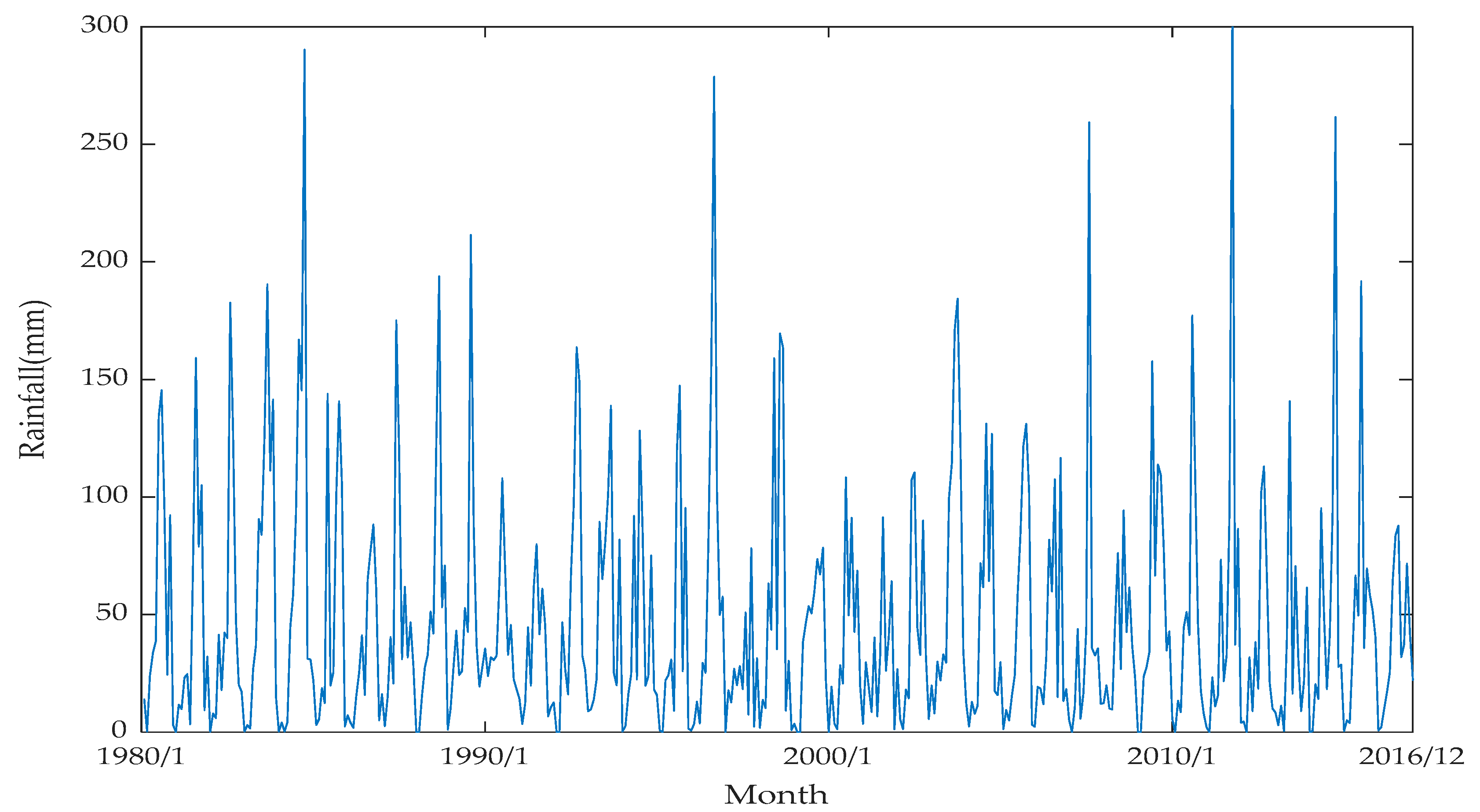
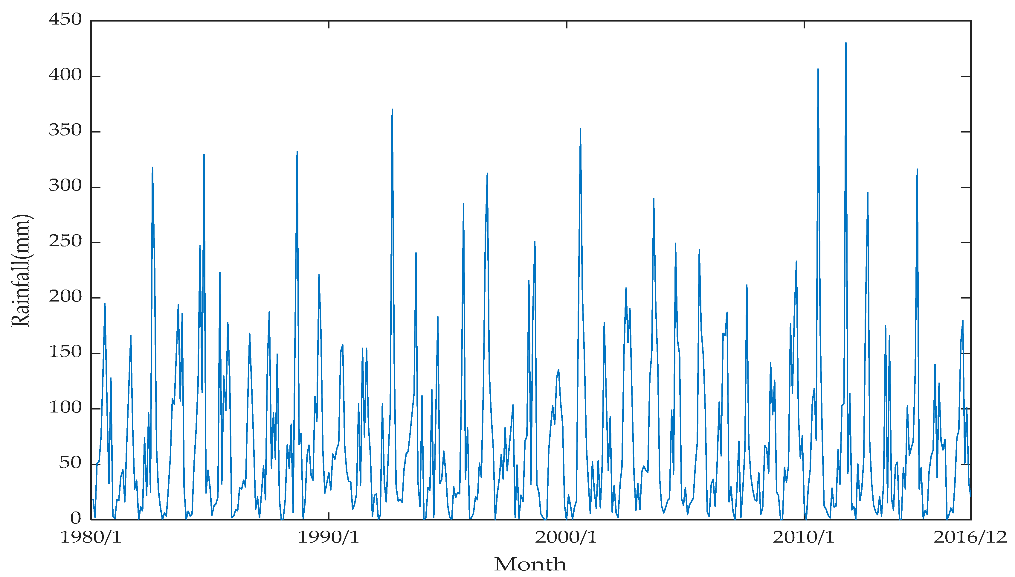
Monthly rainfall data from two stations are used to investigate the accuracy of several prediction methods. Table 1 shows statistical parameters of monthly rainfall data at Luoning and Zuoyu stations. It can be observed that the original data shows obvious standard deviation, indicating a high difficulty of modeling. Figure 2 and Figure 3 present rainfall data for the two stations, where the data run from 1980 to 2016. In this study, data from 1980 to 2013 are used for training and the final three years are utilized for testing.
WPD is used to decompose two observed monthly rainfall series into a series of sub-series. The data of all series are divided into training and testing datasets that are normalized to a range of [0, 1] as
where and are the normalized and the observed value of the i-th data sample, respectively.
2.3. Methods
2.3.1. ARIMA Model
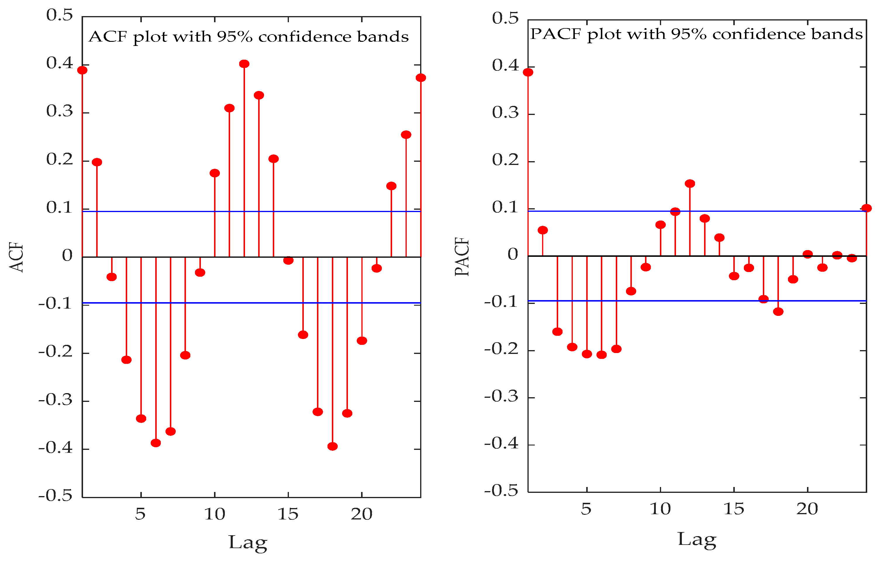
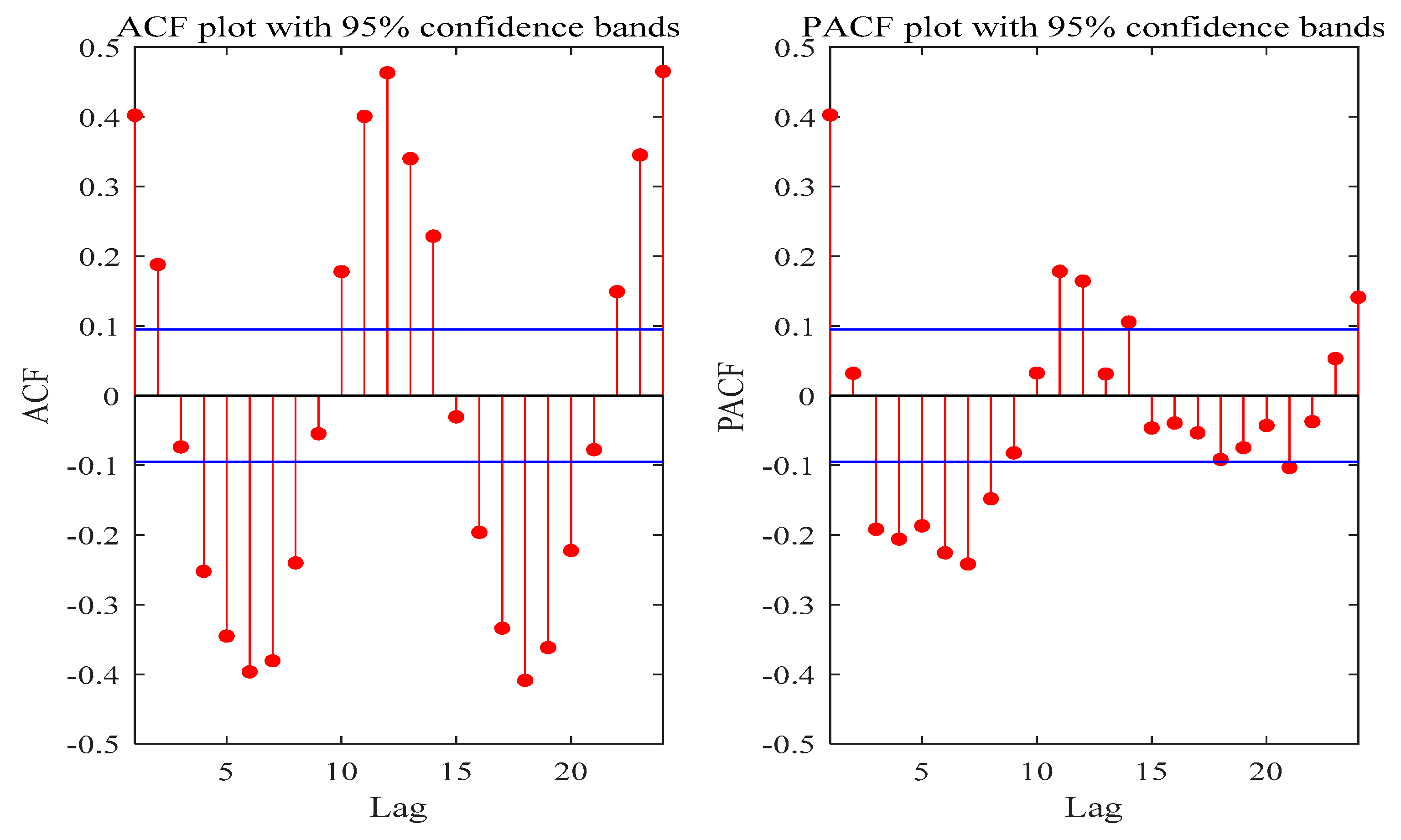
The ARIMA model proposed by Box and Jenkins [15] has been extensively utilized for analyzing and forecasting hydrologic time series [51]. The principle of ARIMA is to use historical times series to find the forecasting noise, so that the data can be processed smoothly, thus solving the random disturbance problem of the series [52]. ARIMA model construction includes six steps: data acquisition, data preprocessing, model identification, model order determination, parameter estimation, and model verification. Two monthly series collected from China are taken as the test cases. Data preprocessing is the test of stationarity of time series. Recently, ACF (autocorrelation function) and PACF (partial autocorrelation function) are generally adopted to test the stationarity of data. In this paper, the Box–Jenkins method is used for model identification, and Bayes information criteria (BIC) method is used for model order determination. In ARIMA (p, d, q), p represents the number of autoregressive terms, is the number of moving average terms, and d is the order of differential.
AR model of order p, which is written as , can be expressed as follows:
The model is:
Thus, the expression of ARMA (p, q) is defined below as:
The ARIMA model is obtained by the d-order difference of the ARMA model. Therefore, the ARIMA (p, d, q) model is:
where represents the predicted value of the model at time , is model coefficient, is previous observation, is model parameter related to white noise, is white noise process that obeys a normal distribution with zero mean and variance , is previous noise term, and , denotes computation according to the above law. Note that can be replaced with only when d = 0.
2.3.2. BPNN Model
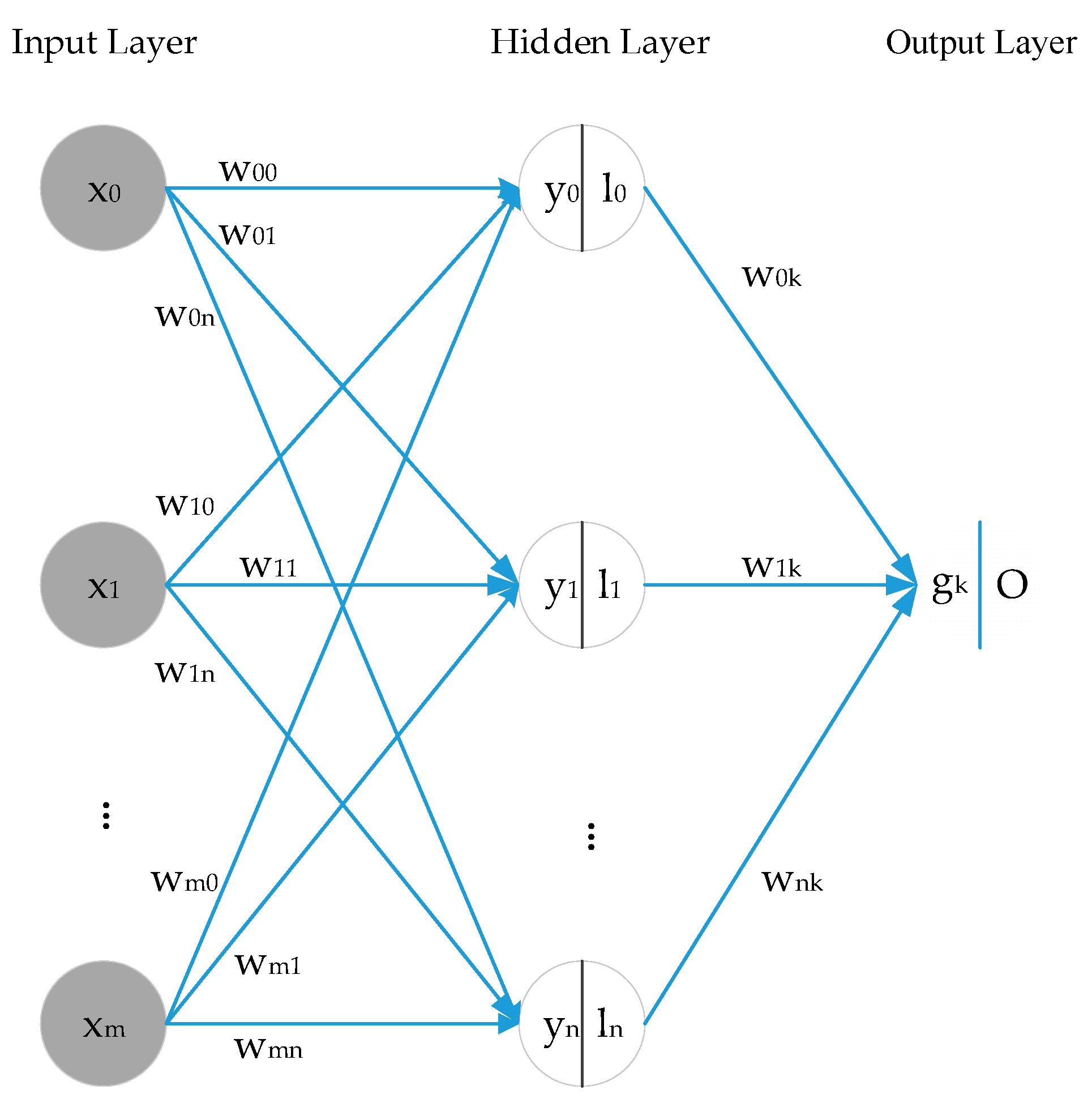
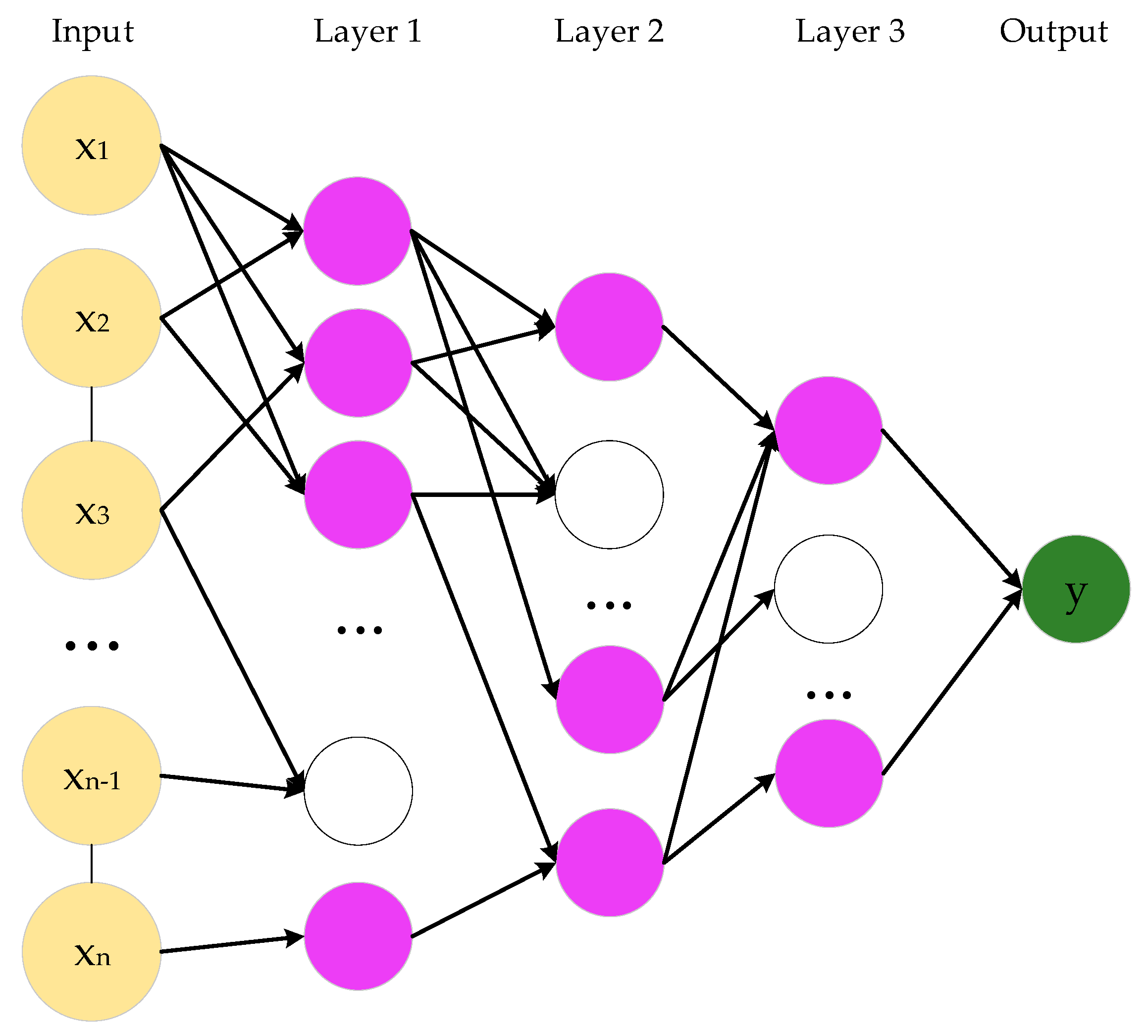
BPNN, proposed by Fausett [53], is a typical multilayer ANN on the basis of error back propagation. BPNN uses the slope reduction method to find the point(s) with minimum error [54]. These three layers, that is, input layer, hidden layer, and output layer, are employed in BPNN (as shown in Figure 4). The signal is input into the network by the input layer and output by the output layer. BPNN adds several layers (one or more layers) of neurons between the input layer and the output layer. These neurons are called hidden layer neurons. They have no direct contact with the outside world, but the change of their state can affect the relationship between input and output. A conventional three-layer BPNN is used to establish the prediction model of monthly precipitation series in this paper. Tan-sigmoid is the transfer function between the output layer and hidden layer, and the nonlinear Levenberg–Marquardt (LM) algorithm is the training function of BPNN.
The mathematical principle of BPNN model is as follows:
where xj is input neuron and j ∈ (0, m), m is the number of input neurons, wij is weight of the ith neuron in the input layer corresponding to the neuron in the hidden layer, is bias-related weight of hidden neurons, yi is input of the hidden layer node (), and n is the number of neurons in the hidden layer. Tan-sigmoid is the transfer function between the layer output and the hidden layer, and its form is as follows:
The output layer is estimated by the following equation:
Among them, gk and represent input and output values of the output layer, respectively.
The formulas above are the principles of the feedforward propagation mode of the BPNN model. In the process of cyclic simulation, errors generated by the system are collected and returned to the output value. By adjusting the weights and thresholds of neurons, network parameters corresponding to the minimum error are determined to generate an ANN system which can simulate the original problem.
2.3.3. GMDH Model
GMDH was developed by Ivakhnenko [55] as a self-organizing approach, which can be applied for multivariate analysis and modeling of complex systems. GMDH has been used to deal with problems of high-order polynomial regression, especially modeling and classification of systems [56]. An important feature of the GMDH method is that external information (i.e., information and data not used in model construction and parameter estimation) is used in modeling, the data of training period is used for modeling, and the information of testing period is only used to select the optimal complexity model. Input and output variables of GMDH are connected by a complex Volterra function in the following form [57]:
where x denotes the input variable of system, is the weight, is output variable, and n is the number of input variables. Many applications in the quadratic form with only two variables are termed partial descriptions, and use the following form to predict output:
The coefficient is obtained by minimizing the Mean Square Error (MSE) between the input–output data pairs:
where N is the sample size of the training set.
The GMDH model adopts the principle of the classic neural network whose signal propagates forward through network nodes. After the weight has been computed, optimal transfer function of the node is obtained and then its output is passed to the next layer of nodes. As shown in Figure 5, the structure of GMDH network is constantly changing during the training process. GMDH will select the input variables that affect the prediction, which means that the connection between neurons in the network is not fixed, but is selected during training to optimize the network structure; The number of layers in the network is also automatically selected to produce maximum accuracy and avoid over fitting. Solid neurons in each layer are selected neurons, and hollow ones represent unselected neurons.
2.3.4. Wavelet Packet Decomposition (WPD)
Mallat [58] proposed a Wavelet Representation (WR) theory to compute and interpret multiresolution representation by decomposing the original signal utilizing orthogonal wavelets. WPD reduces the noise of signal by decomposing the signal into different frequencies, which can be regarded as a special WR. In the procedure of orthogonal wavelet decomposition, the signal is decomposed into approximate coefficients and detail coefficients after passing through multiple filters. When performing the next layer decomposition, the upper low-frequency series and high-frequency series are split into two components, and so on. Wavelet function ψ(t) can be defined as:
The form of SWT (successive wavelet transform) of x(t) is:
where represents the mother wavelet and denotes its complex conjugate, and are the scale expansion parameter and time translation parameter, respectively. In engineering applications, input signal is usually discrete. Let , , j and n denote the frequency localization and time localization. The DWT form of is shown in the following equation:
Normally, we can set and , and this case is the most efficient for practical applications [58]. Therefore Equation (14) becomes the binary orthogonal wavelet transform:
Unlike DWT, WPD passes more filters, which decompose the signal using both high-frequency components and low-frequency components:
where is the scaling function or the approximation coefficients, and is wavelet function (also termed detail coefficient). The two functions correspond to two finite pulse filters, namely, low-pass filter (LPF) and high-pass filter (HPF) . Hence, the equation of orthogonal wavelet packet is:
where and are subject to the following condition:
The wavelet packet function is written by:
The wavelet packet coefficients can be computed by:
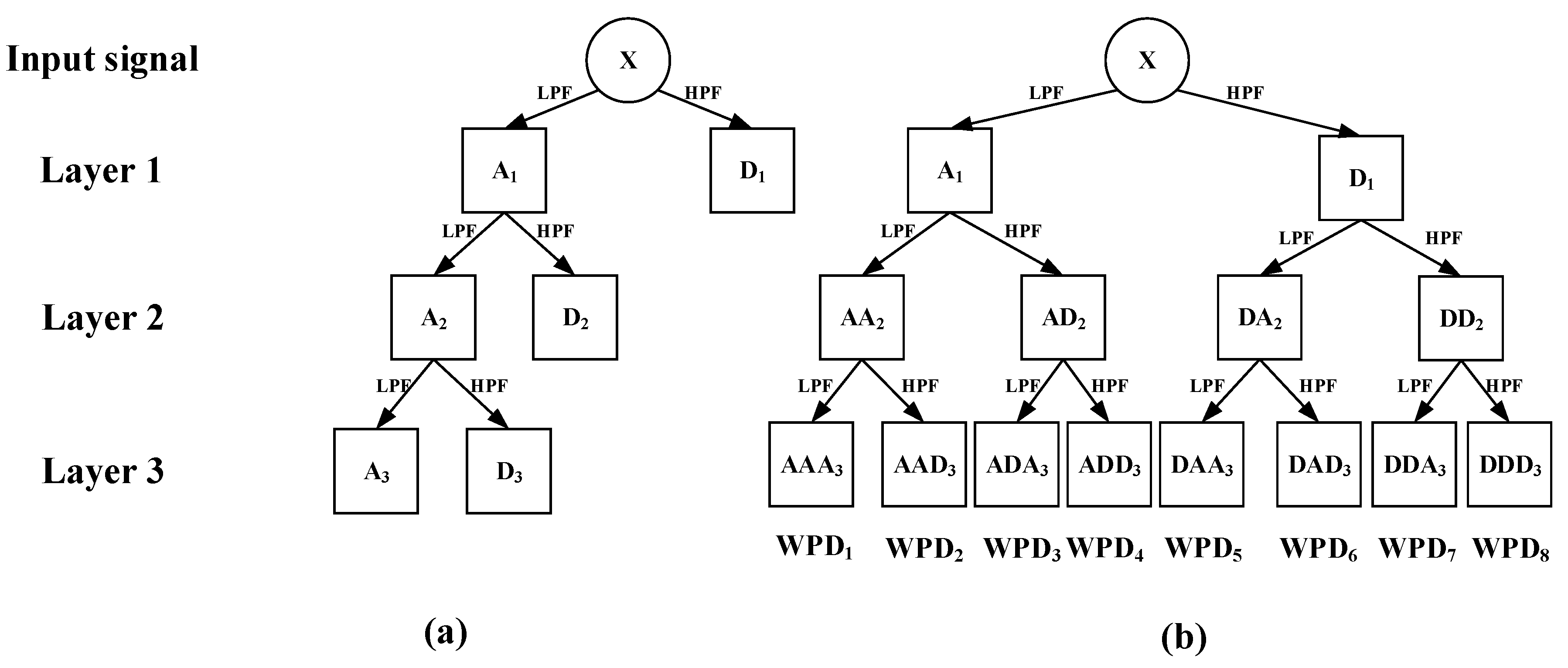
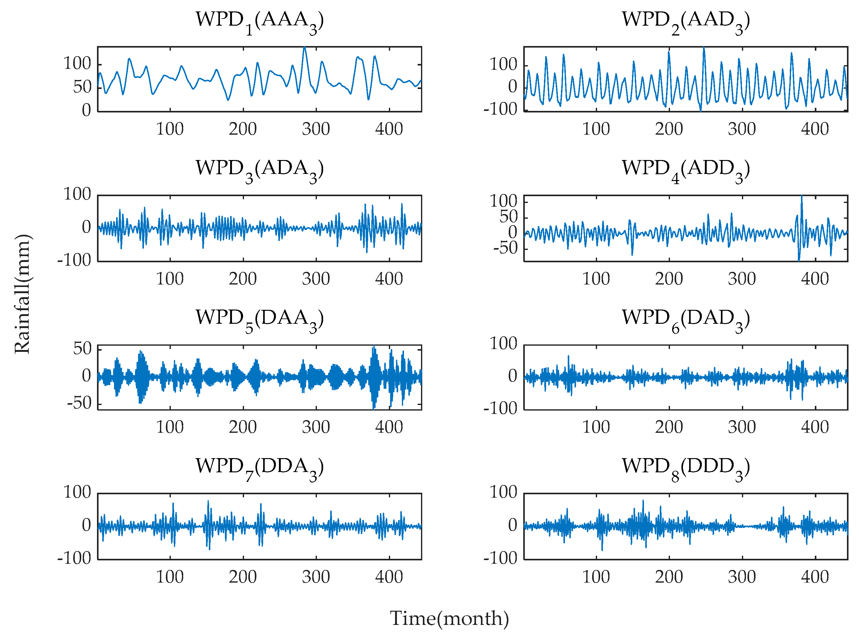
Figure 6 illustrates the binary tree of a three-layer WPD. The original signal is shown by x and each node corresponds to a frequency band. LPF and HPF represent low-pass filter and high-pass filter, respectively. The original signal is decomposed into eight subsequences by a three-level WPD. AAA3 and DDD3 represent the lowest frequency and highest frequency, respectively.
2.4. Evaluation Indices
To evaluate the forecast capacity of different models, four generally adopted standard statistical metrics are used in this study to estimate the global and local errors of models. They are namely RMSE (root mean-squared error) [59], MAE (mean absolute error) [60], R (coefficient of correlation), and NSEC (the Nash–Sutcliffe efficiency coefficient) [61]. RMSE is sensitive even to small errors, which can size the model performance for high rainfall values. However, MAE is suitable for measuring the goodness of fit of model in cases of moderate precipitation. R sizes the degree of collinearity criterion of two variables. NSEC is a widely used index to evaluate the performance measurement of hydrological models. The following formulas are used for computing these parameters:
where and are the observed and predicted rainfall, respectively, and represent their average values, and is the total number of input samples.
2.5. Hybrid Forecasting Models
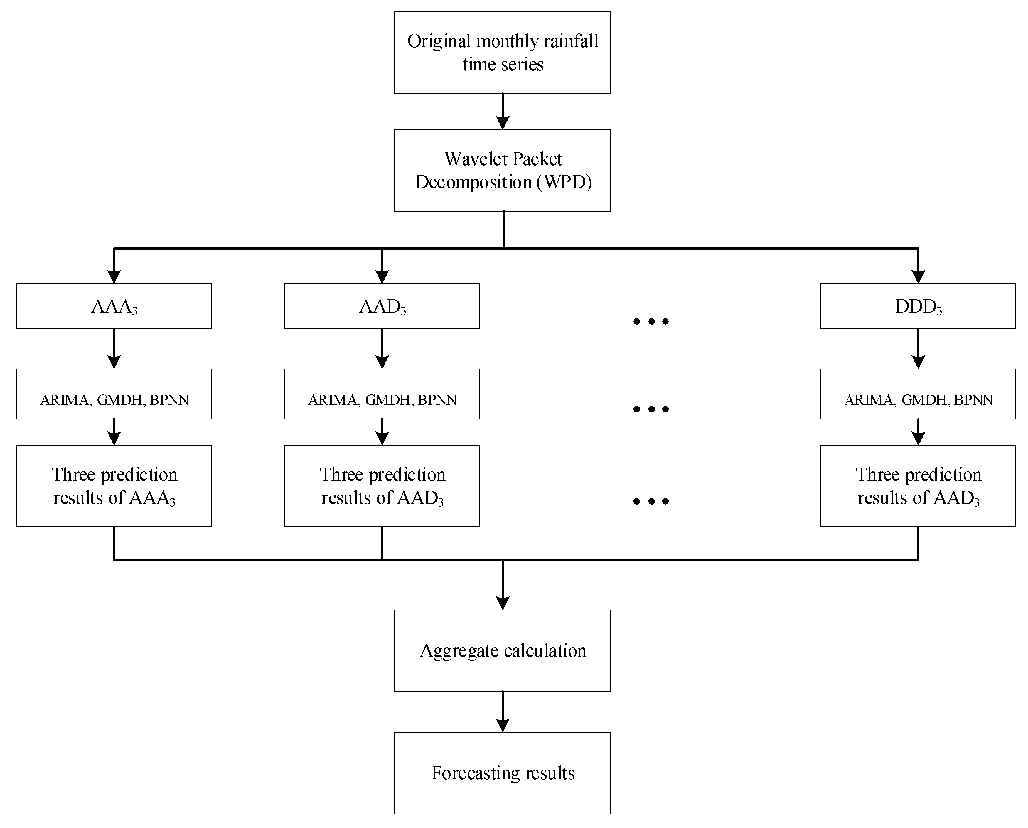
This study investigates the accuracy of ARIMA, BPNN, and GMDH models based on WPD in monthly rainfall forecasting. The framework of hybrid models is showed in Figure 7. It can be summarized from Figure 4 that the main steps of the hybrid model prediction architecture are:
Step 1: Observed monthly rainfall series are decomposed into eight subsequences with different frequencies and spatiotemporal resolutions, four low-frequency series, and four high-frequency series using WPD.
Step 2: In this study, ACF and PACF are employed to select the number of input variables for the model, and then set values of basic model parameters.
Step 3: ARIMA, BPNN, and GMDH models are used as forecasting tools to model and predict each decomposed sub-sequence separately.
Step 4: Finally, the ensemble monthly rainfall forecasting result of model is formulated by summing the outputs of all submodules.
To sum up, the hybrid WPD-ARIMA, WPD-BPNN, and WPD-GMDH forecasting models use the idea of “decomposition and ensemble”. The paper takes 35-year monthly rainfall data from Luoning and Zuoyu stations in Luoyang, China as the test cases.
3. Results
3.1. Decomposition Results Using WPD and Input Variables Determination
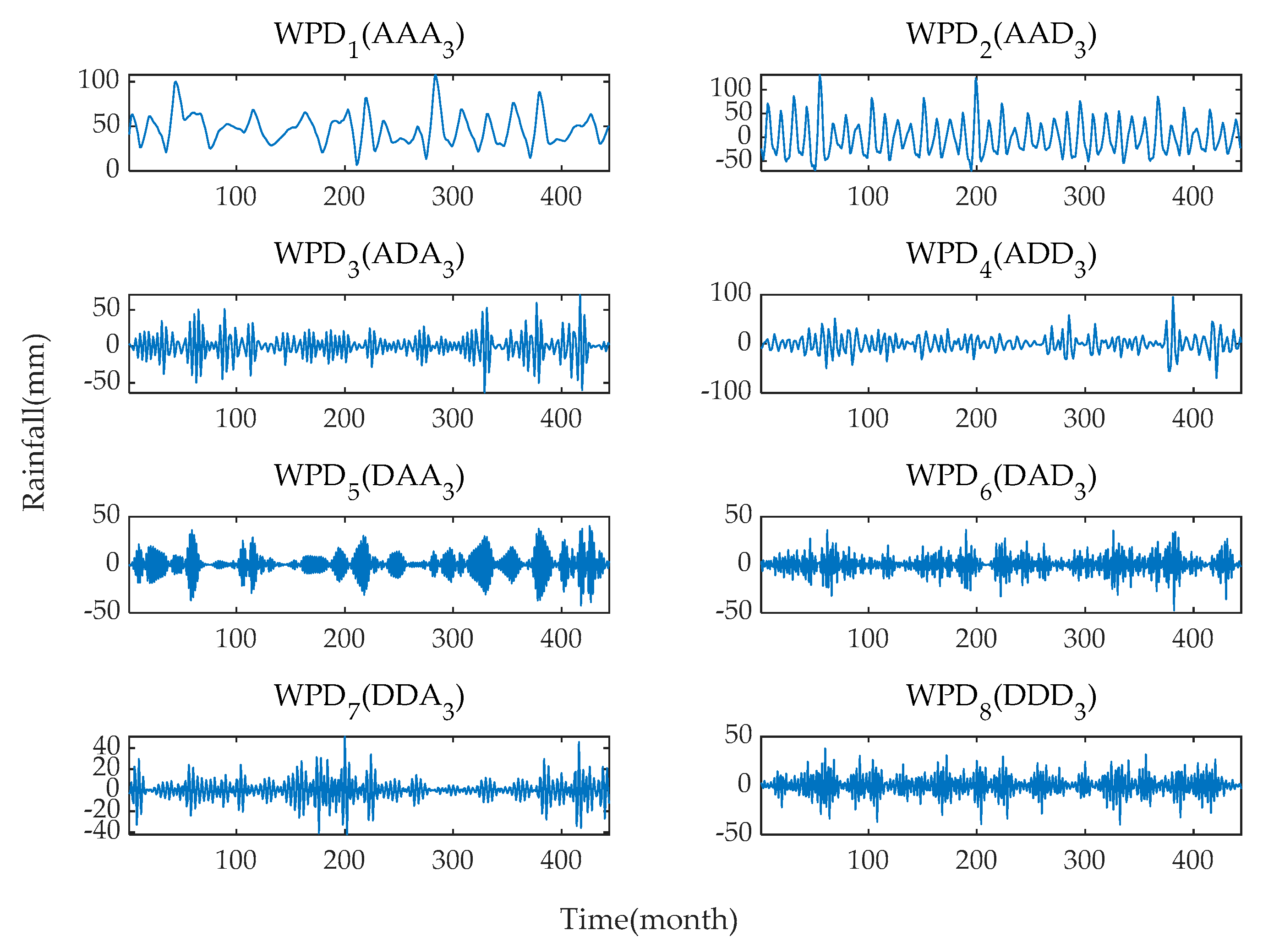
The original monthly rainfall time series are decomposed into eight subsequences with different frequencies and amplitudes using the WPD method. The frequency characteristics of each subsequence are different, and each sub-series plays a different role in the original dataset. The results of WPD of the original monthly rainfall time series data at level 3 are shown in Figure 8 and Figure 9.
Generally, it is very important to set an appropriate number of input variables for data-based prediction models because it is closely related to the characteristics of system to be modeled [62]. In this paper, ACF and PACF are selected as the potential indicators for determining the appropriate input variable. ACF and PACF are normally utilized to pre-determine the sequence of the autoregressive process and modeling of time series [63]. Figure 10 and Figure 11 show ACF and PACF values of the original precipitation series for Luoning and Zuoyu stations, whilst the values of ACF and PACF for all decomposed subseries are not presented here. Referring to ACF and PACF values of the series and influencing factors of precipitation, Table 2 lists input variables of the original series and their subsequences at Luoning and Zuoyu stations. Among them, represents the th variable before the target output variable.
3.2. Model Development
Six models, namely BPNN, WPD-BPNN, GMDH, WPD-GMDH, ARIMA, and WPD-ARIMA models, are employed for benchmark comparison to study the prediction performance of these conjunction methods.
(1) ARIMA
Generally, the ARIMA model based on the difference process is applied to the modeling of non-stationary series. In this paper, the stationarity of the original monthly rainfall series and subsequences are tested by the Augmented Dickey–Fuller (ADF) test. The results of ADF unit root tests are shown in Table 3. The value of the original and all subsequences of the two stations are zero. The p-value of the original sequence and all sub sequences of the two stations is zero, except that the p-value of the original sequence of Zuoyu station is 0.0004. When , p-value < 0.05, and the value of t-statistic is less than the preset upper limit, the null hypothesis is rejected, and the sequence can be considered as stationary; otherwise, the series needs to be differential. It can be seen from Table 3 that the sample set data is stationary series without a single root effect.
The next step is to choose the optimal ARIMA (p, d, q) model, and the best fitted values of p and q are selected according to the BIC method. ACF and PACF are used to predetermine the structure of data sets. Furthermore, referring to the BIC minimum criterion, the best fitting model is determined for the original sequence and the decomposed subsequence of the two stations. The values of p and q are determined based on ACF and PACF, and the significance test has to be passed, that is, when p-value is less than 0.05, select the parameter with minimum BIC statistics. ARIMA models for various sequences are shown in Table 4. The decomposed sub-sequences of Luoning and Zuoyu stations are modeled by the ARIMA model. The original time series are modeled by seasonal ARIMA model (SARIMA), where p, d, and q represent the autoregressive term, the order of difference, and the moving average term of SARIMA model, respectively.
(2) BPNN
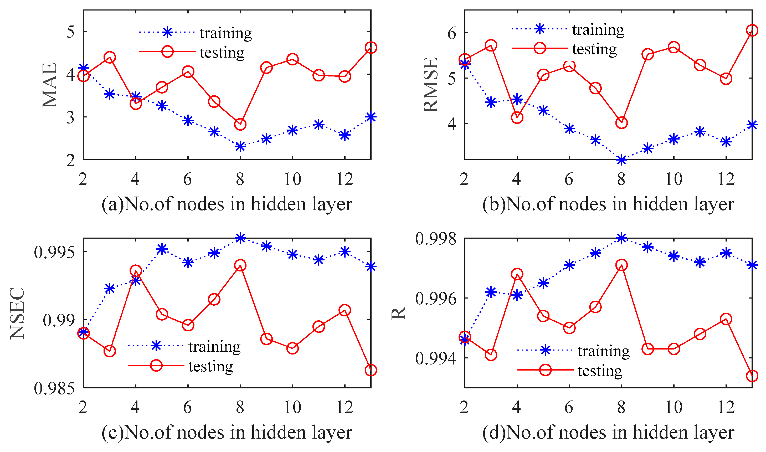
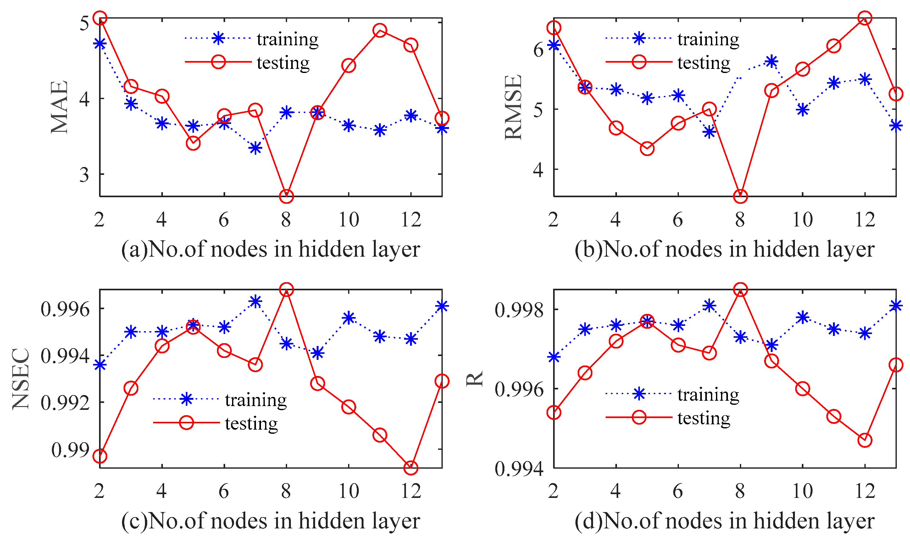
A conventional three-layer BPNN is used to establish the prediction model of monthly precipitation series in this paper. Tan-sigmoid is the transfer function between output and hidden layers, and the nonlinear Levenberg–Marquardt (LM) algorithm is the training function of BPNN. The maximum number of iterations is 100. The number of input layer nodes is the same as the number of input variables. The optimal value is determined by continuously adjusting the number of hidden layer neurons in the range of 2 to 13. The original dataset falls into training samples and test samples. According to the four quantitative indexes, a cross-validation approach is utilized to determine the number of hidden neurons. With the increase of the number of hidden neurons, variations in the statistical indicators of Luoning/Zuoyu station corresponding to different hidden layer nodes are shown in Figure 12 and Figure 13. In this paper, we use to refer to the number of hidden layers. It can be observed from Figure 12 and Figure 13 that is not highly correlated with the performance of BPNN model. For Luoning station, when , RMSE and MSE of training and testing periods are both at a minimum, while R and NSEC reach a maximum. For Zuoyu station, when , MSE and RMSE of the testing set reach the minimum value; meanwhile, NSEC and R attain the maximum value. However, when p is seven, MSE and RMSE of the training set reach the minimum value, NSEC and R of the training set reach the maximum value. Therefore, p is chosen to be eight for both Luoning and Zuoyu stations.
(3) GMDH
The number of input layer nodes is the same as the number of input variables, and then the regression of output value of upper layer is computed to create the second layer network. GMDH uses the best new variables in each layer to build the next layer network. The GMDH model includes three parameters, namely a denoting the maximum number of layers, b denoting the maximum number of nodes in each layer, and p denoting the selection pressure. In this paper, a and b are determined as 3 and 15, respectively, whilst p is set equal to 0.75 via a trial-and-error method, and the convergence criteria is RMSE. This paper determines an appropriate maximum number of hidden layers and nodes of GMDH model by a trial-and-error method. We set equal to 2, 3, and 5, and b equal to 5, 10, and 15. The results (not supplied) show that the numbers of and b have a significant effect on the performance of the GMDH model.
(4) WPD
WPD is adopted for data preprocessing, which can eliminate noises in hydrological time series. The selection of an appropriate mother wavelet is very significant to WPD. The Symlet wavelet function is an improved version of the classical Daubechies wavelet function, which evades the change of waveform in the process of signal decomposition [64]. Therefore, the fourth order Symlet wavelet function is considered as the mother wavelet function. In this paper, three-scale wavelet WPD is selected because large-scale wavelet packet decomposition may lead to information loss.
3.3. Results and Discussion
Based on the above description, different methods are utilized to model the observed rainfall and extracted sub-sequences. Table 5 and Table 6 list the statistical indexes of different algorithms for Luoning and Zuoyu stations during training and testing periods.
For Luoning station, the WPD-BPNN model attains the best RMSE, MAE, R, and NSEC values during the training period, which are 3.292, 2.384, 0.998, and 0.956, respectively. In the testing phase, the WPD-BPNN model also attains the best R, RMSE, MAE, and NSEC statistics of 0.997, 4.054, 2.912, and 0.994, respectively. Meanwhile, for Zuoyu station, the WPD-BPNN model attains the best RMSE, MAE, R, and NSEC values during the training period, which are 5.935, 4.102, 0.997, and 0.994, respectively. In analyzing the results during the testing phase, the WPD-BPNN model attains the best R, RMSE, MAE, and NSEC statistics of 0.998, 3.705, 2.889, and 0.996, respectively. Referring to the four evaluation indicators in this paper, WPD-BPNN can attain the best performance in monthly precipitation prediction.
Table 7 and Table 8 list the comparison of results on model prediction performance by different indicators. When forecasting monthly rainfall at Luoning station, WPD-BPNN is able to attain the best improving capability of RMSE and MAE in the training phase, while WPD-GMDH is able to attain the best improving capability of R and NSEC in the training phase. In analyzing the figures during the testing phase, WPD-BPNN attains the best improving capability of RMSE and MAE, while WPD-ARIMA attains the best improving capability of R and NSEC. In addition, it can be seen from Table 8 that the prediction performance of the models is similar for Zuoyu and Luoning stations. Therefore, the monthly rainfall series decomposed by WPD method as the input of BPNN model can drastically improve the forecasting accuracy. This reaffirms the superior performance of WPD. Furthermore, the enhancement capabilities of different evaluation methods are different in terms of different phases and different forecasting measures.
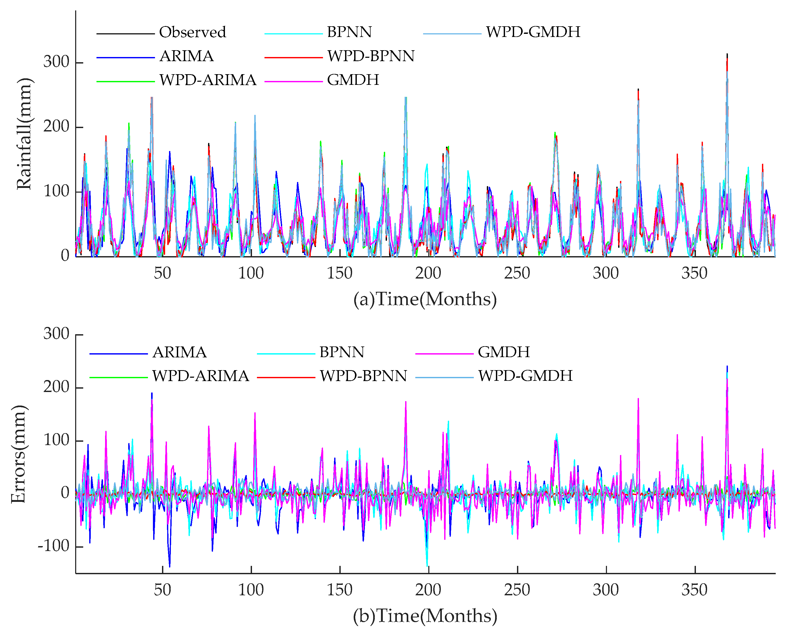
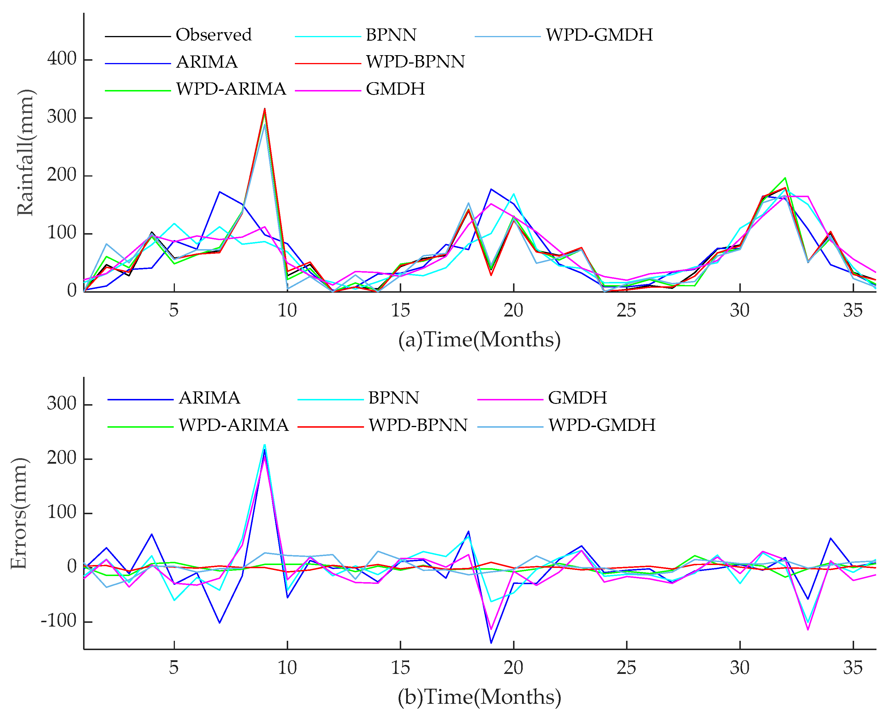
For the two research objects in this paper, the performance of all models during training and test periods are shown in Figure 14, Figure 15, Figure 16, Figure 17. The performances of hybrid models for monthly rainfall simulation are able to attain better performance than those of conventional ARIMA, BPNN, and GMDH methods. WPD-BPNN presents the best performance, and its trend line is almost perfectly close to the smooth line of the observed data. In contrast, there are huge deviations between the prediction results obtained by ARIMA, BPNN, and GMDH methods and observed data. In addition, the prediction values of the extreme points of the three single models are far less than the observed value, and the peak prediction also has an obvious lag effect. However, compared with ARIMA, GMDH, and BPNN, the three WPD-based models have greatly improved the peak value accuracy and time positioning. Meanwhile, the models prior to improvement cannot capture abrupt changes of precipitation in rainy season. Therefore, compared with several existing methods in this paper, WPD-BPNN is the most efficient tool for monthly rainfall forecasting, since it can achieve excellent prediction results.
4. Conclusions
In recent years, the improvement of hydrological forecasting accuracy has attracted widespread attention around the world. In order to broaden the scope of hydrological forecasting theory, this study explores the performance of several data-driven methods based on WPD in monthly precipitation forecasting. Firstly, the observed monthly rainfall time series are decomposed into eight subsequences with different frequencies and spatiotemporal resolutions by WPD. Then, three data-based models, namely BPNN, GMDH, and ARIMA models, are utilized to complete the prediction for the decomposed monthly rainfall series, respectively. Finally, the ensembled prediction result of the model is formulated by summing the outputs of all submodules. Monthly rainfall data from two stations in China are utilized to test the performance of these methods. To evaluate the forecast capacity of different models, four standard statistical metrics are adopted to estimate the global and local errors of the models.
The results reveal that the WPD model is suitable for the decomposition of monthly rainfall series, and WPD-BPNN can provide the best performance during both training and testing periods in terms of the four evaluation indicators in this paper. The following briefly introduces the advantages of the WPD-BPNN method. Firstly, the principle of WPD is simple and inclusive, and it can comprehensively and deeply analyze the characteristics of monthly precipitation series. Secondly, the prediction performance of BPNN only depends on the characteristics of input variables. Finally, the proposed model does not require complex decision-making for the explicit form of the model in different cases. Therefore, the hybrid forecast model based on WPD technology is an efficient tool to improve the accuracy of mid- and long-term rainfall forecasting.
It should be pointed out that, although this paper has fully verified the feasibility of WPD-BPNN in monthly precipitation forecasting, there are still several limitations to be explored in the future research. Firstly, the study is carried out based on two time series, so we will test the generalization of the proposed model. The second is to test the performance of other algorithms combined with WPD. The last major issue is to develop an appropriate optimization algorithm to improve the performance of WPD-BPNN. In future research, it is necessary to conduct in-depth research on the three aspects above to explore more efficient and accurate forecasting techniques and make contributions to the field of hydrological forecasting.
Author Contributions
W.W.: Conceptualization, Methodology, Writing—original draft. Y.D.: Program implementation, data curation, Writing—original draft preparation. K.C.: Writing and editing—original draft. H.C.: Writing—original draft. C.L.: Investigation. Q.M.: Formal analysis. All authors have read and agreed to the published version of the manuscript.
Funding
The project of Key Science and Technology of the Henan province (202102310259; 202102310588), and the Henan province University Scientific and Technological Innovation team (No: 18IRTSTHN009).
Institutional Review Board Statement
Not applicable.
Informed Consent Statement
Not applicable.
Data Availability Statement
All authors made sure that all data and materials support our published claims and comply with field standards.
Conflicts of Interest
The authors declare that they have no conflict of interest.
Abbreviations
| WPD | wavelet packet decomposition |
| BPNN | back-propagation neural network |
| GMDH | group method of data handing |
| ARIMA | autoregressive integrated moving average |
| ANN | artificial neural network |
| GP | genetic programming |
| SVM | support vector machines |
| ANFIS | adaptive neuro-fuzzy inference system |
| AR | auto-regressive |
| MA | moving average |
| ARMA | autoregressive moving average |
| LM | Levenberg–Marquardt |
| EMD | empirical mode decomposition |
| EEMD | ensemble empirical mode decomposition |
| FT | Fourier transform |
| SVR | support vector regression |
| QPSO | quantum-behaved particle swarm optimization |
| VMD | variational mode decomposition |
| LSWA | least-squares wavelet analysis |
| WD | wavelet decomposition |
| DWT | discrete wavelet transform |
| WR | wavelet representation |
| LPF | low-pass filter |
| HPF | high-pass filter |
| RMSE | root mean-squared error |
| MAE | mean absolute error |
| R | coefficient of correlation |
| NSEC | Nash–Sutcliffe efficiency coefficient |
| ACF | autocorrelation function |
| PACF | partial autocorrelation function |
| ADF | augmented Dickey–Fuller |
| BIC | Bayes information criteria |
| SCS-CN | soil conservation service-curve number |
References
- Adnan, R.M.; Liang, Z.; Heddam, S.; Zounemat-Kermani, M.; Kisi, O.; Li, B. Least square support vector machine and multivariate adaptive regression splines for streamflow prediction in mountainous basin using hydro-meteorological data as inputs. J. Hydrol. 2020, 586, 124371. [Google Scholar] [CrossRef]
- Ghaderpour, E.; Vujadinovic, T.; Hassan, Q.K. Application of the Least-Squares Wavelet software in hydrology: Athabasca River Basin. J. Hydrol. Reg. Stud. 2021, 36, 100847. [Google Scholar] [CrossRef]
- Kisi, O.; Cimen, M. A wavelet-support vector machine conjunction model for monthly streamflow forecasting. J. Hydrol. 2011, 399, 132–140. [Google Scholar] [CrossRef]
- Niu, W.-J.; Feng, Z.-K.; Chen, Y.-B.; Zhang, H.; Cheng, C.-T. Annual Streamflow Time Series Prediction Using Extreme Learning Machine Based on Gravitational Search Algorithm and Variational Mode Decomposition. J. Hydrol. Eng. 2020, 25, 04020008. [Google Scholar] [CrossRef]
- Ali, M.; Prasad, R.; Xiang, Y.; Yaseen, Z.M. Complete ensemble empirical mode decomposition hybridized with random forest and kernel ridge regression model for monthly rainfall forecasts. J. Hydrol. 2020, 584, 124647. [Google Scholar] [CrossRef]
- Yang, T.; Asanjan, A.A.; Welles, E.; Gao, X.; Sorooshian, S.; Liu, X. Developing reservoir monthly inflow forecasts using artificial intelligence and climate phenomenon information. Water Resour. Res. 2017, 53, 2786–2812. [Google Scholar] [CrossRef]
- Wang, W.-C.; Xu, D.-M.; Chau, K.-W.; Chen, S. Improved annual rainfall-runoff forecasting using PSO-SVM model based on EEMD. J. Hydroinform. 2013, 15, 1377–1390. [Google Scholar] [CrossRef]
- Wang, W.-C.; Cheng, C.-T.; Chau, K.-W.; Xu, D.-M. Calibration of Xinanjiang model parameters using hybrid genetic algorithm based fuzzy optimal model. J. Hydroinform. 2012, 14, 784–799. [Google Scholar] [CrossRef] [Green Version]
- Abbaszadeh, P.; Alipour, A. Development of a coupled wavelet transform and evolutionary Levenberg-Marquardt neural networks for hydrological process modeling. Comput. Intell. 2018, 34, 175–199. [Google Scholar] [CrossRef]
- Wang, W.-C.; Chau, K.-W.; Cheng, C.-T.; Qiu, L. A comparison of performance of several artificial intelligence methods for forecasting monthly discharge time series. J. Hydrol. 2009, 374, 294–306. [Google Scholar] [CrossRef] [Green Version]
- Aksoy, H.; Dahamsheh, A. Artificial neural network models for forecasting monthly precipitation in Jordan. Stoch. Environ. Res. Risk Assess. 2009, 23, 917–931. [Google Scholar] [CrossRef]
- Chadalawada, J.; Herath, H.; Babovic, V. Hydrologically Informed Machine Learning for Rainfall-Runoff Modeling: A Genetic Programming-Based Toolkit for Automatic Model Induction. Water Resour. Res. 2020, 56, e2019WR026933. [Google Scholar] [CrossRef]
- Sain, S.R. The Nature of Statistical Learning Theory. Technometrics 1996, 38, 409. [Google Scholar] [CrossRef]
- Jang, J.R. ANFIS: Adaptive-network-based fuzzy inference system. IEEE Trans. Syst. Man Cybern. 1993, 23, 665–685. [Google Scholar] [CrossRef]
- Box, G.; Jenkins, G. Time Series Analysis-Forecast and Control; Prentice-Hall: Englewood Cliffs, NJ, USA, 1976. [Google Scholar]
- Lai, Y.; Dzombak, D.A. Use of the Autoregressive Integrated Moving Average (ARIMA) Model to Forecast Near-Term Regional Temperature and Precipitation. Weather Forecast. 2020, 35, 959–976. [Google Scholar] [CrossRef]
- Mishra, A.K.; Desai, V.R. Drought forecasting using stochastic models. Stoch. Environ. Res. Risk Assess. 2005, 19, 326–339. [Google Scholar] [CrossRef]
- Sanikhani, H.; Kisi, O.; Maroufpoor, E.; Yaseen, Z.M. Temperature-based modeling of reference evapotranspiration using several artificial intelligence models: Application of different modeling scenarios. Theor. Appl. Climatol. 2019, 135, 449–462. [Google Scholar] [CrossRef]
- Rahman, M.A.; Lou, Y.S.; Sultana, N. Analysis and prediction of rainfall trends over Bangladesh using Mann-Kendall, Spearman′s rho tests and ARIMA model. Meteorol. Atmos. Phys. 2017, 129, 409–424. [Google Scholar] [CrossRef]
- Mishra, S.; Saravanan, C.; Dwivedi, V.K.; Shukla, J.P. Rainfall-Runoff Modeling using Clustering and Regression Analysis for the River Brahmaputra Basin. J. Geol. Soc. India 2018, 92, 305–312. [Google Scholar] [CrossRef]
- Rizeei, H.M.; Pradhan, B.; Saharkhiz, M.A. Surface runoff prediction regarding LULC and climate dynamics using coupled LTM, optimized ARIMA, and GIS-based SCS-CN models in tropical region. Arab. J. Geosci. 2018, 11, 53. [Google Scholar] [CrossRef]
- Wang, Z.-Y.; Qiu, J.; Li, F.-F. Hybrid Models Combining EMD/EEMD and ARIMA for Long-Term Streamflow Forecasting. Water 2018, 10, 853. [Google Scholar] [CrossRef] [Green Version]
- Tan, Q.-F.; Lei, X.-H.; Wang, X.; Wang, H.; Wen, X.; Ji, Y.; Kang, A.-Q. An adaptive middle and long-term runoff forecast model using EEMD-ANN hybrid approach. J. Hydrol. 2018, 567, 767–780. [Google Scholar] [CrossRef]
- Kashani, M.H.; Ghorbani, M.A.; Shahabi, M.; Naganna, S.R.; Diop, L. Multiple AI model integration strategy—Application to saturated hydraulic conductivity prediction from easily available soil properties. Soil Tillage Res. 2020, 196, 104449. [Google Scholar] [CrossRef]
- Pradhan, P.; Tingsanchali, T.; Shrestha, S. Evaluation of Soil and Water Assessment Tool and Artificial Neural Network models for hydrologic simulation in different climatic regions of Asia. Sci. Total Environ. 2020, 701, 134308. [Google Scholar] [CrossRef]
- Dubey, S.K.; Sharma, D.; Babel, M.S.; Mundetia, N. Application of hydrological model for assessment of water security using multi-model ensemble of CORDEX-South Asia experiments in a semi-arid river basin of India. Ecol. Eng. 2020, 143, 105641. [Google Scholar] [CrossRef]
- Gokbulak, F.; Sengonul, K.; Serengil, Y.; Yurtseven, I.; Ozhan, S.; Cigizoglu, H.K.; Uygur, B. Comparison of Rainfall-Runoff Relationship Modeling using Different Methods in a Forested Watershed. Water Resour. Manag. 2015, 29, 4229–4239. [Google Scholar] [CrossRef]
- Nourani, V. An Emotional ANN (EANN) approach to modeling rainfall-runoff process. J. Hydrol. 2017, 544, 267–277. [Google Scholar] [CrossRef]
- Malekzadeh, M.; Kardar, S.; Saeb, K.; Shabanlou, S.; Taghavi, L. A Novel Approach for Prediction of Monthly Ground Water Level Using a Hybrid Wavelet and Non-Tuned Self-Adaptive Machine Learning Model. Water Resour. Manag. 2019, 33, 1609–1628. [Google Scholar] [CrossRef]
- Mukherjee, A.; Ramachandran, P. Prediction of GWL with the help of GRACE TWS for unevenly spaced time series data in India: Analysis of comparative performances of SVR, ANN and LRM. J. Hydrol. 2018, 558, 647–658. [Google Scholar] [CrossRef]
- Choong, C.E.; Ibrahim, S.; El-Shafie, A. Artificial Neural Network (ANN) model development for predicting just suspension speed in solid-liquid mixing system. Flow Meas. Instrum. 2020, 71, 101689. [Google Scholar] [CrossRef]
- Mokhtarzad, M.; Eskandari, F.; Jamshidi Vanjani, N.; Arabasadi, A. Drought forecasting by ANN, ANFIS, and SVM and comparison of the models. Environ. Earth Sci. 2017, 76, 729. [Google Scholar] [CrossRef]
- Vidyarthi, V.K.; Jain, A. Knowledge extraction from trained ANN drought classification model. J. Hydrol. 2020, 585, 124804. [Google Scholar] [CrossRef]
- Liu, Y.; Zhao, Q.; Yao, W.; Ma, X.; Yao, Y.; Liu, L. Short-term rainfall forecast model based on the improved BP–NN algorithm. Sci. Rep. 2019, 9, 19751. [Google Scholar] [CrossRef] [PubMed]
- Danladi, A.; Stephen, M.; Aliyu, B.M.; Gaya, G.K.; Silikwa, N.W.; Machael, Y. Assessing the influence of weather parameters on rainfall to forecast river discharge based on short-term. Alex. Eng. J. 2018, 57, 1157–1162. [Google Scholar] [CrossRef]
- Cui, Y.K.; Long, D.; Hong, Y.; Zeng, C.; Zhou, J.; Han, Z.Y.; Liu, R.H.; Wan, W. Validation and reconstruction of FY-3B/MWRI soil moisture using an artificial neural network based on reconstructed MODIS optical products over the Tibetan Plateau. J. Hydrol. 2016, 543, 242–254. [Google Scholar] [CrossRef]
- Yuan, Q.; Xu, H.; Li, T.; Shen, H.; Zhang, L. Estimating surface soil moisture from satellite observations using a generalized regression neural network trained on sparse ground-based measurements in the continental U.S. J. Hydrol. 2020, 580, 124351. [Google Scholar] [CrossRef]
- Amanifard, N.; Nariman-Zadeh, N.; Farahani, M.H.; Khalkhali, A. Modelling of multiple short-length-scale stall cells in an axial compressor using evolved GMDH neural networks. Energy Convers. Manag. 2008, 49, 2588–2594. [Google Scholar] [CrossRef]
- Li, Y.; Shi, H.; Liu, H. A hybrid model for river water level forecasting: Cases of Xiangjiang River and Yuanjiang River, China. J. Hydrol. 2020, 587, 124934. [Google Scholar] [CrossRef]
- Adnan, R.M.; Liang, Z.; Parmar, K.S.; Soni, K.; Kisi, O. Modeling monthly streamflow in mountainous basin by MARS, GMDH-NN and DENFIS using hydroclimatic data. Neural Comput. Appl. 2021, 33, 2853–2871. [Google Scholar] [CrossRef]
- Partal, T.; Kişi, Ö. Wavelet and neuro-fuzzy conjunction model for precipitation forecasting. J. Hydrol. 2007, 342, 199–212. [Google Scholar] [CrossRef]
- Wang, W.-C.; Chau, K.-W.; Qiu, L.; Chen, Y.-B. Improving forecasting accuracy of medium and long-term runoff using artificial neural network based on EEMD decomposition. Environ. Res. 2015, 139, 46–54. [Google Scholar] [CrossRef] [PubMed]
- Yu, X.; Zhang, X.; Qin, H. A data-driven model based on Fourier transform and support vector regression for monthly reservoir inflow forecasting. J. Hydro-Environ. Res. 2018, 18, 12–24. [Google Scholar] [CrossRef]
- Feng, Z.-K.; Niu, W.-J.; Tang, Z.-Y.; Jiang, Z.-Q.; Xu, Y.; Liu, Y.; Zhang, H.-R. Monthly runoff time series prediction by variational mode decomposition and support vector machine based on quantum-behaved particle swarm optimization. J. Hydrol. 2020, 583, 124627. [Google Scholar] [CrossRef]
- Deering, R.; Kaiser, J.F. The use of a masking signal to improve empirical mode decomposition. In Proceedings of the (ICASSP’05): IEEE International Conference on Acoustics, Speech, and Signal Processing, Philadelphia, PA, USA, 23 March 2005; Volume 484, pp. iv/485–iv/488. [Google Scholar]
- Chong, K.L.; Lai, S.H.; El-Shafie, A. Wavelet Transform Based Method for River Stream Flow Time Series Frequency Analysis and Assessment in Tropical Environment. Water Resour. Manag. 2019, 33, 2015–2032. [Google Scholar] [CrossRef]
- Bayazit, M. Nonstationarity of Hydrological Records and Recent Trends in Trend Analysis: A State-of-the-art Review. Environ. Process. 2015, 2, 527–542. [Google Scholar] [CrossRef]
- Coifman, R.; Meyer, Y.; Wickerhauser, V.M. Wavelet analysis and signal processing. In Wavelets and Their Applications; Jones Bartlett: Burlington, MA, USA, 1992; pp. 153–178. [Google Scholar]
- Cohen, A.; Daubechies, I.; Feauveau, J.C. Biorthogonal bases of compactly supported wavelets. Commun. Pure Appl. Math. 1992, 45, 485–560. [Google Scholar] [CrossRef]
- Zhao, L.; Jia, Y. Transcale control for a class of discrete stochastic systems based on wavelet packet decomposition. Inf. Sci. 2015, 296, 25–41. [Google Scholar] [CrossRef]
- Unnikrishnan, P.; Jothiprakash, V. Hybrid SSA-ARIMA-ANN Model for Forecasting Daily Rainfall. Water Resour. Manag. 2020, 34, 3609–3623. [Google Scholar] [CrossRef]
- Lu, Y.; AbouRizk, S.M. Automated Box–Jenkins forecasting modelling. Autom. Constr. 2009, 18, 547–558. [Google Scholar] [CrossRef]
- Fausett, L. Fundamentals of Neural Networks: Architectures, Algorithms, and Applications; Prentice-Hall Inc.: Upper Saddle River, NJ, USA, 1994. [Google Scholar]
- Yang, Z.P.; Lu, W.X.; Long, Y.Q.; Li, P. Application and comparison of two prediction models for groundwater levels: A case study in Western Jilin Province, China. J. Arid Environ. 2009, 73, 487–492. [Google Scholar] [CrossRef]
- Ivakhnenko, A. Polynomial theory of complex systems. IEEE Trans. Syst. Man Cybern. 1971, 1, 364–378. [Google Scholar] [CrossRef] [Green Version]
- Qaderi, K.; Bakhtiari, B.; Madadi, M.R.; Afzali-Gorouh, Z. Evaluating GMDH-based models to predict daily dew point temperature (case study of Kerman province). Meteorol. Atmos. Phys. 2020, 132, 667–682. [Google Scholar] [CrossRef]
- Volterra, V. Theory of Functionals and of Integrals and Integro-Differential Equations; Dover Publications: New York, NY, USA, 2005. [Google Scholar]
- Mallat, S.; Mallat, S.G. A Theory of Multiresolution Signal Decomposition: The Wavelet Representation. IEEE Trans. Pattern Anal. Mach. Intell. 1989, 11, 674–693. [Google Scholar] [CrossRef] [Green Version]
- Gentilucci, M.; Materazzi, M.; Pambianchi, G.; Burt, P.; Guerriero, G. Assessment of Variations in the Temperature-Rainfall Trend in the Province of Macerata (Central Italy), Comparing the Last Three Climatological Standard Normals (1961–1990; 1971–2000; 1981–2010) for Biosustainability Studies. Environ. Process. 2019, 6, 391–412. [Google Scholar] [CrossRef]
- Wang, W.; Lu, Y. Analysis of the Mean Absolute Error (MAE) and the Root Mean Square Error (RMSE) in Assessing Rounding Model. IOP Conf. Ser. Mater. Sci. Eng. 2018, 324, 012049. [Google Scholar] [CrossRef]
- Kim, H.I.; Keum, H.J.; Han, K.Y. Real-Time Urban Inundation Prediction Combining Hydraulic and Probabilistic Methods. Water 2019, 11, 293. [Google Scholar] [CrossRef] [Green Version]
- Feng, Q.; Wen, X.; Li, J. Wavelet Analysis-Support Vector Machine Coupled Models for Monthly Rainfall Forecasting in Arid Regions. Water Resour. Manag. 2015, 29, 1049–1065. [Google Scholar] [CrossRef]
- Lin, J.-Y.; Cheng, C.-T.; Chau, K.-W. Using support vector machines for long-term discharge prediction. Hydrol. Sci. J. 2006, 51, 599–612. [Google Scholar] [CrossRef]
- Yin, Y.; Bai, Y.; Ge, F.; Yu, H.; Liu, Y. Long-term robust identification potential of a wavelet packet decomposition based recursive drift correction of E-nose data for Chinese spirits. Measurement 2019, 139, 284–292. [Google Scholar] [CrossRef]
Figure 1.
Location of Luoning and Zuoyu stations.

Figure 2.
Monthly rainfall time series at Luoning station.

Figure 3.
Monthly rainfall time series at Zuoyu station.

Figure 4.
Schematic diagram of a BPNN structure.

Figure 5.
Schematic diagram of a GMDH network structure.

Figure 6.
Three-layer structure diagram: (a) WD; (b) WPD.

Figure 7.
The framework of hybrid models.

Figure 8.
Decomposed results for monthly rainfall at Luoning station.

Figure 9.
Decomposed results for monthly rainfall at Zuoyu station.

Figure 10.
ACF and PACF values for the original data series from Luoning station.

Figure 11.
ACF and PACF values for the original data series from Zuoyu station.

Figure 12.
Variation of statistical indicators with the number of hidden layer nodes for Luoning station.
Figure 12.
Variation of statistical indicators with the number of hidden layer nodes for Luoning station.

Figure 13.
Variation of statistical indicators with the number of hidden layer nodes for Zuoyu station.
Figure 13.
Variation of statistical indicators with the number of hidden layer nodes for Zuoyu station.

Figure 14.
(a) Forecasting results of Luoning station in the training period; (b) forecasting errors of Luoning station in the training period.
Figure 14.
(a) Forecasting results of Luoning station in the training period; (b) forecasting errors of Luoning station in the training period.

Figure 15.
(a) Forecasting results of Luoning station in the testing period; (b) forecasting errors of Luoning station in the testing period.
Figure 15.
(a) Forecasting results of Luoning station in the testing period; (b) forecasting errors of Luoning station in the testing period.

Figure 16.
(a) Forecasting results of Zuoyu station in training period; (b) forecasting errors of Zuoyu station in the training period.
Figure 16.
(a) Forecasting results of Zuoyu station in training period; (b) forecasting errors of Zuoyu station in the training period.

Figure 17.
(a) Forecasting results of Zuoyu station in testing period; (b) forecasting errors of Luoning station in the testing period.
Figure 17.
(a) Forecasting results of Zuoyu station in testing period; (b) forecasting errors of Luoning station in the testing period.


Table 1.
Statistical parameters of monthly rainfall data at Luoning and Zuoyu stations.
| Station | Max (mm) | Min (mm) | Mean (mm) | Std (mm) | |
|---|---|---|---|---|---|
| Luoning | All | 313.8 | 0 | 47.18 | 50.93 |
| Training | 313.8 | 0 | 47.05 | 50.86 | |
| Testing | 261.7 | 0.4 | 48.66 | 52.39 | |
| Zuoyu | All | 430.2 | 0 | 69.53 | 74.39 |
| Training | 430.2 | 0 | 69.92 | 75.33 | |
| Testing | 316.2 | 0 | 65.05 | 63.44 |
Note: Max is the maximum, Min is the minimum, Std is the standard deviation.
Table 2.
Number of input variables for different data series from Luoning and Zuoyu stations based on ACF and PACF analysis.
Table 2.
Number of input variables for different data series from Luoning and Zuoyu stations based on ACF and PACF analysis.
| No. | Series | Input Variables | |
|---|---|---|---|
| Luoning Station | Zuoyu Station | ||
| 1 | Original | xt−1~xt−12 | xt−1~xt−13 |
| 2 | WPD1 | xt−1~xt−12 | xt−1~xt−12 |
| 3 | WPD2 | xt−1~xt−12 | xt−1~xt−12 |
| 4 | WPD3 | xt−1~xt−12 | xt−1~xt−13 |
| 5 | WPD4 | xt−1~xt−11 | xt−1~xt−11 |
| 6 | WPD5 | xt−1~xt−12 | xt−1~xt−12 |
| 7 | WPD6 | xt−1~xt−12 | xt−1~xt−12 |
| 8 | WPD7 | xt−1~xt−13 | xt−1~xt−13 |
| 9 | WPD8 | xt−1~xt−11 | xt−1~xt−13 |
Table 3.
ADF test in the sample data set.
| Name | Sample Data Set | t-Statistic Value | Critical Value |
|---|---|---|---|
| Luoning | Original | −5.85207 | −3.42041 |
| WPD1 | −6.70412 | −3.42041 | |
| WPD2 | −14.33 | −3.42041 | |
| WPD3 | −12.6215 | −3.42041 | |
| WPD4 | −16.2217 | −3.42041 | |
| WPD5 | −9.58776 | −3.42041 | |
| WPD6 | −18.1806 | −3.42041 | |
| WPD7 | −14.919 | −3.42041 | |
| WPD8 | −24.0394 | −3.42041 | |
| Zuoyu | Original | −4.86539 | −3.42041 |
| WPD1 | −6.63558 | −3.42041 | |
| WPD2 | −14.6596 | −3.42041 | |
| WPD3 | −12.2977 | −3.42041 | |
| WPD4 | −16.5301 | −3.42041 | |
| WPD5 | −10.0685 | −3.42041 | |
| WPD6 | −17.6399 | −3.42041 | |
| WPD7 | −14.3801 | −3.42041 | |
| WPD8 | −25.9766 | −3.42041 |
Table 4.
The structure of each sequence.
| Name | Sample Data Set | ARIMA (p, d, q)/SARIMA (p, d, q) (P, D, Q) | BIC |
|---|---|---|---|
| Luoning | Original | SARIMA (5,1,1) (1,1,1) | 7.602 |
| WPD1 | ARIMA (2,1,3) | 1.005 | |
| WPD2 | ARIMA (2,0,8) | 4.016 | |
| WPD3 | ARIMA (2,0,7) | 2.091 | |
| WPD4 | ARIMA (3,0,5) | 3.333 | |
| WPD5 | ARIMA (5,0,7) | −0.274 | |
| WPD6 | ARIMA (2,0,7) | 1.469 | |
| WPD7 | ARIMA (2,0,7) | 1.098 | |
| WPD8 | ARIMA (6,0,8) | 1.132 | |
| Zuoyu | Original | SARIMA (5,1,1) (1,1,1) | 8.119 |
| WPD1 | ARIMA (2,0,5) | 1.469 | |
| WPD2 | ARIMA (3,0,3) | 4.844 | |
| WPD3 | ARIMA (2,0,8) | 2.209 | |
| WPD4 | ARIMA (2,0,8) | 2.992 | |
| WPD5 | ARIMA (10,0,7) | -0.128 | |
| WPD6 | ARIMA (3,0,8) | 1.745 | |
| WPD7 | ARIMA (2,0,7) | 1.43 | |
| WPD8 | ARIMA (6,0,4) | 2.229 |
Table 5.
Forecasting performance indices of models for Luoning station.
| Model | Training | Testing | ||||||
|---|---|---|---|---|---|---|---|---|
| R | RMSE | MAE | NSEC | R | RMSE | MAE | NSEC | |
| ARIMA | 0.608 | 40.926 | 27.442 | 0.352 | 0.459 | 46.474 | 27.792 | 0.191 |
| WPD-ARIMA | 0.984 | 9.210 | 7.298 | 0.967 | 0.988 | 8.224 | 6.060 | 0.975 |
| BPNN | 0.667 | 37.896 | 25.913 | 0.445 | 0.484 | 45.775 | 29.204 | 0.215 |
| WPD-BPNN | 0.998 | 3.296 | 2.384 | 0.996 | 0.997 | 4.054 | 2.912 | 0.994 |
| GMDH | 0.584 | 41.299 | 28.495 | 0.340 | 0.600 | 41.844 | 24.575 | 0.344 |
| WPD-GMDH | 0.970 | 12.372 | 9.588 | 0.941 | 0.966 | 13.734 | 11.171 | 0.929 |
Table 6.
Forecasting performance indices of models for Zuoyu station.
| Model | Training | Testing | ||||||
|---|---|---|---|---|---|---|---|---|
| R | RMSE | MAE | NSEC | R | RMSE | MAE | NSEC | |
| ARIMA | 0.679 | 55.717 | 38.124 | 0.459 | 0.576 | 53.689 | 31.856 | 0.263 |
| WPD-ARIMA | 0.987 | 12.455 | 9.525 | 0.973 | 0.992 | 7.970 | 6.415 | 0.984 |
| BPNN | 0.709 | 53.518 | 36.089 | 0.500 | 0.607 | 50.37 | 31.846 | 0.352 |
| WPD-BPNN | 0.997 | 5.935 | 4.102 | 0.994 | 0.998 | 3.705 | 2.889 | 0.996 |
| GMDH | 0.662 | 56.751 | 39.460 | 0.433 | 0.643 | 48.271 | 30.439 | 0.405 |
| WPD-GMDH | 0.973 | 17.771 | 13.970 | 0.945 | 0.980 | 14.797 | 11.623 | 0.944 |
Table 7.
Comparison of results of model prediction performance for Luoning station.
| Model | Index | Training (%) | Testing (%) |
|---|---|---|---|
| WPD-ARIMA & ARIMA | R(↑) | 61.81 | 115.48 |
| NSEC(↑) | 174.54 | 732.71 | |
| RMSE(↓) | 77.5 | 80.3 | |
| MAE(↓) | 73.4 | 78.19 | |
| WPD-BPNN & BPNN | R(↑) | 45.52 | 106.8 |
| NSEC(↑) | 123.98 | 362.45 | |
| RMSE(↓) | 91.3 | 91.14 | |
| MAE(↓) | 90.8 | 90.3 | |
| WPD-GMDH & GMDH | R(↑) | 66.22 | 61.17 |
| NSEC(↑) | 176.38 | 170.22 | |
| RMSE(↓) | 70.04 | 74.35 | |
| MAE(↓) | 66.35 | 54.54 |
Note: (↑) represents the percentage of performance improvement of the new model compared to the original model, and (↓) represents the percentage of performance reduction of the new model compared to the original model.
Table 8.
Comparison of results of model prediction performance for Zuoyu station.
| Model | Index | Training (%) | Testing (%) |
|---|---|---|---|
| WPD-ARIMA&ARIMA | R(↑) | 45.34 | 72.08 |
| NSEC(↑) | 105.30 | 273.50 | |
| RMSE(↓) | 77.65 | 85.15 | |
| MAE(↓) | 75.02 | 79.86 | |
| WPD-BPNN&BPNN | R(↑) | 40.53 | 64.51 |
| NSEC(↑) | 98.86 | 183.50 | |
| RMSE(↓) | 88.91 | 92.64 | |
| MAE(↓) | 88.63 | 90.93 | |
| WPD-GMDH&GMDH | R(↑) | 46.81 | 52.33 |
| NSEC(↑) | 118.32 | 133.37 | |
| RMSE(↓) | 68.69 | 69.35 | |
| MAE(↓) | 64.60 | 61.82 |
Note: where (↑) represents the percentage of performance improvement of the new model compared to the original model, and (↓) represents the percentage of performance reduction of the new model compared to the original model.
Publisher’s Note: MDPI stays neutral with regard to jurisdictional claims in published maps and institutional affiliations. |
© 2021 by the authors. Licensee MDPI, Basel, Switzerland. This article is an open access article distributed under the terms and conditions of the Creative Commons Attribution (CC BY) license (https://creativecommons.org/licenses/by/4.0/).
Share and Cite
MDPI and ACS Style
Wang, W.; Du, Y.; Chau, K.; Chen, H.; Liu, C.; Ma, Q. A Comparison of BPNN, GMDH, and ARIMA for Monthly Rainfall Forecasting Based on Wavelet Packet Decomposition. Water 2021, 13, 2871. https://doi.org/10.3390/w13202871
AMA Style
Wang W, Du Y, Chau K, Chen H, Liu C, Ma Q. A Comparison of BPNN, GMDH, and ARIMA for Monthly Rainfall Forecasting Based on Wavelet Packet Decomposition. Water. 2021; 13(20):2871. https://doi.org/10.3390/w13202871
Chicago/Turabian StyleWang, Wenchuan, Yujin Du, Kwokwing Chau, Haitao Chen, Changjun Liu, and Qiang Ma. 2021. "A Comparison of BPNN, GMDH, and ARIMA for Monthly Rainfall Forecasting Based on Wavelet Packet Decomposition" Water 13, no. 20: 2871. https://doi.org/10.3390/w13202871
Note that from the first issue of 2016, this journal uses article numbers instead of page numbers. See further details here.