
Evaluation of the RF-Based Downscaled SMAP and SMOS Products Using Multi-Source Data over an Alpine Mountains Basin, Northwest China


1
College of Geography and Environmental Science, Northwest Normal University, Lanzhou 730070, China
2
State Key Laboratory of Cryosphere Science, Northwest Institute of Eco-Environment and Resources, Chinese Academy of Sciences, Lanzhou 730070, China
*
Author to whom correspondence should be addressed.
Water 2021, 13(20), 2875; https://doi.org/10.3390/w13202875
Submission received: 6 September 2021
/
Revised: 11 October 2021
/
Accepted: 12 October 2021
/
Published: 14 October 2021
(This article belongs to the Topic Recent Advances in Hydroinformatics: Focusing on Machine Learning and Remote Sensing in Hydrology)
Abstract
:Passive microwave surface soil moisture (SSM) products tend to have very low resolution, which massively limits their application and validation in regional or local-scale areas. Many climate and hydrological studies are urgently needed to evaluate the suitability of satellite SSM products, especially in alpine mountain areas where soil moisture plays a key role in terrestrial atmospheric exchanges. Aiming to overcome this limitation, a downscaling method based on random forest (RF) was proposed to disaggregate satellite SSM products. We compared the ability of the downscaled soil moisture active passive (SMAP) SSM and soil moisture and ocean salinity satellite (SMOS) SSM products to capture soil moisture information in upstream of the Heihe River Basin by using in situ measurements, the triple collocation (TC) method and temperature vegetation dryness index (TVDI). The results showed that the RF downscaling method has strong applicability in the study area, and the downscaled results of the two products after residual correction have more details, which can better represent the spatial distribution of soil moisture. The validation with the in situ SSM measurements indicates that the correlation between downscaled SMAP and in situ SSM is better than downscaled SMOS at both point and watershed scales in the Babaohe River Basin. From the TC method, the root mean square error (RMSE) of the CLDAS (CMA land data assimilation system), downscaled SMAP and downscaled SMOS were 0.0265, 0.0255 and 0.0317, respectively, indicating that the downscaled SMAP has smaller errors in the study area than others. However, the soil moisture distribution in the study area shown by the SMOS downscaled results is closer than the downscaled SMAP to the degree of drought reflected by TVDI. Overall, this study suggests that the proposed RF-based downscaling method can capture the variation of SSM well, and the downscaled SMAP products perform significantly better than the downscaled SMOS products after the accuracy verification and error analysis of the downscaled results, and it should be helpful to facilitate applications for satellite SSM products at small scales.
Keywords:
downscaling; random forest; SMAP; SMOS; surface soil moisture; triple collocation; validation1. Introduction
Soil moisture is a key variable in hydrological, ecological and biogeochemical processes. It plays an important role in the evaporation, irrigation and seepage of surface water [1,2,3,4,5]. Long-term observations of soil moisture over large areas are essential for numerous climate and hydrological studies [6,7,8,9] and accurate knowledge of the spatiotemporal behavior of soil moisture can greatly improve hydrological forecasting capability [10,11]. It can be obtained from various methods: in situ measurement from ground meteorological stations [12,13], data assimilation products based on surface models [14], and real-time remote sensing monitoring [15,16]. Due to the large spatial heterogeneity of soil moisture, the station-based soil moisture cannot represent the soil moisture characteristics of the whole large areas [17,18]. Therefore, it is important to use remote sensing technology to dynamically monitor and obtain large-scale soil moisture data in near real-time. Compared with optical/thermal infrared remote sensing, microwave bands can penetrate the atmosphere and clouds to achieve all-weather and all-day observations, and are more sensitive to soil moisture information [19,20]. Therefore, microwave remote sensing has been dedicated to monitoring SSM, including the missions: SMOS(soil moisture and ocean salinity) [21,22] and AMSR-E(advanced microwave scanning radiometer) [23], SMAP(soil moisture active passive mission) [24,25,26], AMSR-2(advanced microwave scanning radiometer-2) [8,27] and FY(Feng Yun) [28,29] series of satellites launched by China. However, such low spatial resolution products cannot meet the application research of hydrological modeling, land surface process, and soil drought prediction in small and medium-scale areas [1], it is necessary to obtain higher spatial resolution and more accurate soil moisture data through downscaling to provide accurate soil moisture data while reducing the difficulty of ground verification.
The relationship between LST and vegetation index can form a ‘universal triangle’ and based on the correlation between SSM and soil moisture status can express soil moisture status, so many empirical regression methods and physics-based models are proposed to construct the relationship model between optical/TIR observations and SSM based on these theories [30]. Chauhan et al. [31] used the 25 km spatial resolution of the soil moisture product retrieved by SSM/I and the optical sensor AVHRR 1 km resolution to establish a statistical regression relationship, downscaled the soil moisture spatial resolution from 25 to 1 km. ChoiandHur [32] downscaled AMSR-E soil moisture products to 1 km in the entire South Korea region. They found the correlation coefficient and root mean square error between the in situ data and the SSM with a spatial resolution of 1 km is better than the SSM product with 25 km. However, these statistical analyses all assume that the distribution of the linear regression relationship is spatially consistent, so local characteristics are ignored. Brunsdon introduced geographic location information and proposed the concept of geographically weighted regression(GWR) to improve the global regression model [33,34,35]. However, it is not suitable to obtain multiple factors to downscale soil moisture because of the limitations of the GWR algorithm. In addition, linear numerical expressions cannot fully represent the complex nonlinear relationship between SSM and other surface variables. Under the premise that the physical mechanism is not yet clear, it is a better choice to use machine learning methods to build downscaling models.
Compared with machine learning methods, such as artificial neural networks and support vector machines, the random forest (RF) algorithm has the advantages of small amount of calculation and large number of samples, and is suitable for remote sensing downscaling research [36]. Imetal. [37] initiated a downscaling research method by introducing machine learning methods to establish complex relationships between soil moisture data from AMSR-E and other MODIS(moderate-resolution imaging spectroradiometer) surface variables products. The result showed the RF method can accurately describe the relationship between AMSR-E and MODIS products. Park et al. [38] used MODIS products closely related to soil moisture and downscaled AMSR2 soil moisture to 1 km by statistical ordinary least square method (OLS) and RF machine learning. RF (R2 = 0.96, RMSE = 0.06) was superior to OLS (R2 = 0.47, RMSE = 0.16) in simulating soil moisture.
The authenticity test of the results obtained by downscaling is a necessary means to objectively evaluate the accuracy, stability and consistency of remote sensing products, however solving the problem of spatial scale mismatch between in situ data and remote sensing data is still a major challenge. The original method of estimating the error of soil moisture data from remote sensing observation uses the observation data of ground stations as the true value estimate the remote sensing observation data. However, the point-scale soil moisture data provided by the ground station cannot represent the regional-scale soil moisture data, and the layout of the station observation is relatively sparse, and it is impossible to obtain large-scale data, which limits this method. Another widely used error estimation is the triple collocation (TC) method, which was proposed by Stoffelen in 1998 and applied to marine sciences to evaluate wind and wave height observations [39]. Compared with the original method, the TC technique was found more appropriate as an upscaling approach capable of compensating for the impact of random measurement error on ground-based measurements [40]. In TC, the random error variances and signal to noise ratios (SNR) of three independent datasets for the same geophysical variable can be estimated without considering any of them as hypothetically error-free references [41]. Draper et al. [42] used TC and error propagation of soil moisture inversion model to estimate the errors of ASCAT data and AMSR-E (LPRM inversion algorithm) data, and the results showed that the two error estimation methods had a high consistency in spatial distribution, and the error estimates of soil moisture data of each land cover type were in line with expectations. It is found through experiments that TC method has good robustness.
Western China is a typical cold and arid region. As an important inland river basin, Heihe River Basin has a unique multi-level natural landscape with water as the link, which has a great influence on regional eco-hydrology in western China. The Qilian Mountains in the upstream of the Heihe River Basin provide a large amount of living and ecological water for the middle and lower reaches of the Heihe River Basin. Therefore, providing high-resolution soil moisture of the upstream of the Heihe River Basin, which can lay a foundation for the research on soil moisture in the alpine mountain area.
On the basis of the above studies, the purpose of this study is to evaluate and comparing the applicability of the downscaled results of SMAP and SMOS soil moisture products obtained by the RF regression method in the upstream of Heihe River Basin. Based on the verification results, soil moisture products with better application were selected for subsequent soil moisture research. First, RF downscaling model was constructed for downscaling two passive microwave SSM products from tens of kilometers to 1 km. Then the prediction performance and results of the RF downscaling model were analyzed, and three verification methods was used to comprehensively evaluate the accuracy, error, and spatio-temporal distribution characteristics of the downscaled results. Finally, the applicability of SMOS and SMAP downscaled soil moisture with high-resolution were analyzed based on the evaluation results in alpine mountains, which providing data support for the follow-up soil moisture research in the study area.
2. Study Area and Data
2.1. Study Area
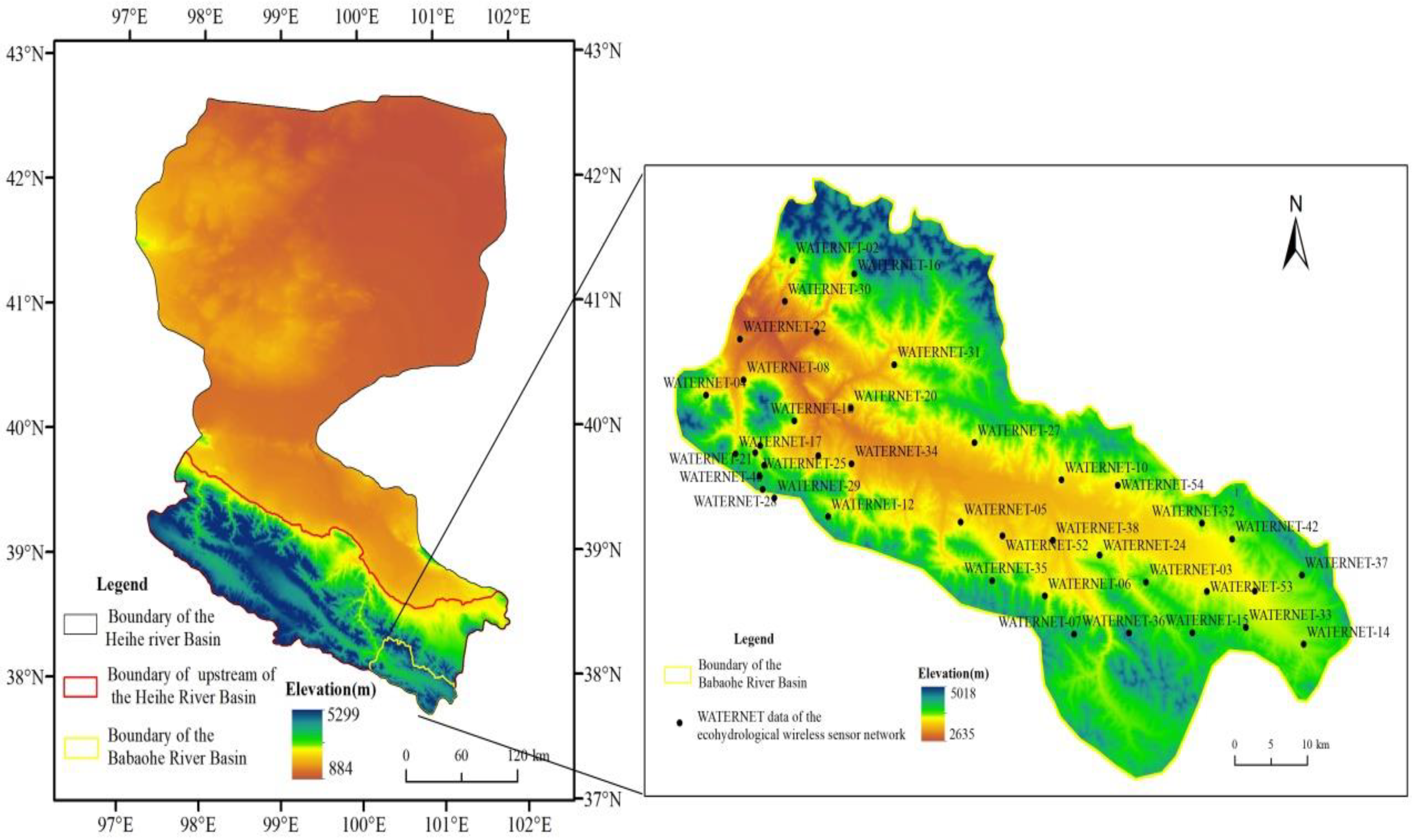
Heihe River Basin is located in the middle of the Hexi Corridor, and is the second-largest inland basin in Northwest China. The upstream of Heihe River Basin is located in the middle part of Qilian Mountains, with a main range of 37.5~39.7° N and 97.5~101.5° E, covering an area of about 10,009 km2 (Figure 1). The whole upstream of Heihe River has an altitude range of 1674~5544 m, with complex terrain and large undulating mountains. The annual precipitation in this region is more, mainly concentrated in summer and autumn, both the annual average temperature and annual evaporation is low. Vegetation types and soil properties showed obvious vertical zone differentiation and the main soil types are loam and sandy loam mixed soil. The upstream of Heihe River basin contains many sub-basins, among which Babaohe River basin is located in the east of the upstream of Heihe River, with an area of about 2452 km2, regional coordinates 37.7~38.3° N, 100~101.3° E. As a typical area of runoff generation in the arid alpine mountains of Northwest China, accurate simulation of the hydrological processes in this area will provide insights for successful hydrological modeling of other similar mountain basins [43].
2.2. Data
2.2.1. In Situ Soil Moisture Observations
In 2013, HIWATER (Heihe Watershed Allied Telemetry Experimental Research) observation test was carried out in the upstream of the Heihe River Basin in the alpine mountains, providing soil temperature, humidity and moisture observations. The observation depths were 0~4, 4~10 and 10~40 cm, and the observation frequency was 5 min/time [44]. In this study, the soil moisture observations data used to evaluate the authenticity of two products were 0~4 cm depth and from the ecohydrological wireless sensor network in the upstream of the Heihe River Basin in 2015 (Figure 1). The total number of nodes used to evaluate two products is 25, as only 25 of the original 40 nodes were left in 2015 due to instrument malfunctions or loss (Table 1) [45,46,47]. The CLDAS data used in this article is the average value within one hour before and after the satellite transit time, and the average value was calculated for validation if multiple nodes exist in a grid cell. The in situ observation data from the HIWATER were downloaded from National Qinghai–Tibet Plateau Data Center (TPDC) website http://data.tpdc.ac.cn/ (accessed on 10 October 2019).
2.2.2. Satellite Soil Moisture Data Products
The SMAP satellite was launched on 31 January 2015 by NASA and designed to monitor global soil moisture changes [48]. It uses L-band radar (active) and radiometer (passive), which is most sensitive to surface water, with a temporal resolution of 2~3 days. It is a satellite in near-polar orbit with the ascending and descending overpass times of 6:00 p.m. and 6:00 a.m. at local time. As the surface and plant heat balance conditions in the morning are closer to the assumed conditions of remote sensing product algorithm [49], the quality of SMAP descending data is usually better than ascending [50]. Therefore, the SMAP Level-2 (L2) passive soil moisture product (SPL2SMP, Version 7) with 36 km spatial resolution from 31 March 2015 to 1 November 2017 was selected in this study. It is available from the EARTHDATA website https://search.earthdata.nasa.gov/ (accessed on 16 June 2020) for the whole dataset.
The Soil Moisture and Ocean Salinity Satellite (SMOS) was launched on November 2009 and began providing data on January 2010, it also carries an L-band microwave radiometer [51]. Due to the good heat balance conditions in the morning, this study selected SMOS L2 descending soil moisture product SMOS_L2_SM_D with a time resolution of 3 days and a spatial resolution of 43 km on average. The SMOS L2 soil moisture data also from 31 March 2015 to 1 November 2017 was used for this research. It can be achieved from the free access to https://smos-diss.eo.esa.int/socat/SMOS_Open (accessed on 20 August 2020).
Not all SMAP and SMOS data downloaded of the study area were of good quality because of various factors, there were some data filled only part of values even empty in the study area. These data have been filtered and deleted to ensure that the SMOS and SMAP data used for RF downscaling are almost fully covered in the study area with good quality.
2.2.3. Soil Moisture Reanalysis Products
CMA land data assimilation system (CMA) is a data assimilation system developed by China Meteorological Information Center. The dataset is developed by using the space and time mesoscale analysis system (STMAS), optimal interpolation (OI), cumulative distribution function (CDF), physical inversion, terrain correction and other technologies. Its quality in China is better than that of similar international products, and its spatial and temporal resolution is higher. The data used in this study is the CLDAS-V2.0, which covers the Asian region (0–65° N, 60–160° E), with a time resolution of 1 h and a spatial resolution of 0.0625° × 0.0625°. The product vertically divided into 5 layers (0–5, 0–10, 10–40, 40–100, 100–200 cm). It can be downloaded from the Basic Data Service of Scientific Expedition to the Qinghai–Tibet Plateau website http://tipex.data.cma.cn (accessed on 30 October 2020).
2.2.4. MODIS Products
The MODIS satellites Terra and Aqua operate on a solar synchronous polar orbit. The Terra and Aqua have different overpass times which are 10:30 AM of Terra and 13:30 PM of Aqua, respectively. Over the past few years, among many surface variables, vegetation index and land surface temperature (LST) have been widely used to downscale satellite soil moisture data [37,52]. In this study, MODIS land surface temperature (LST) and NDVI (normalized difference vegetation index) of the Terra with descending daytime overpass were chosen to be consistent with the data acquisition time of SMAP and SMOS data. In addition, the MODIS products that were utilized in this study also including surface albedo (ALB), leaf area index (LAI), evapotranspiration (ET), these surface variables have been demonstrated the potential in expressing their relationship with SSM. Therefore, all these MODIS surface variables products from March 31, 2015 to November 1, 2017 were selected in this study and obtained from the LAADS DAAC of NASA website https://ladsweb.modaps.eosdis.nasa.gov/ (accessed on 17 June 2020), including the daily LST (MOD11A1) with 1 km resolution, 16 day NDVI (MOD13A2) with 1 km resolution, daily albedo (MCD43A3) with1 km resolution, MODIS/Terra 8-Day LAI (MCD15A2) with 500 m resolution, and 8 day ET (MOD16A2) with 500 m resolution.
2.2.5. Topographic Data
In addition to the above satellite data, the processes SRTM digital elevation model (DEM) data with a resolution of 250 m resolution was also selected in this study, and it was obtained from the Geospatial Data Cloud website http://www.gscloud.cn/sources/ (accessed on 5 September 2019). To make it the same resolution as MODIS products, it was aggregated by Bilinear interpolation to get the same resolution (1 km) as other variables and used to provide topographic factors (elevation and slope) for the downscaling study.
3. Methods
3.1. Random Forest Downscaling Method
The random forest machine learning model is based on decision tree proposed by Breiman and Cutler [53], which is used to solve tasks such as classification and regression. The RF method is an ensemble learning model that utilizes multiple weak classifiers (decision trees) to improve generalization ability and reduce over-fitting phenomena. In a regression, the mean predicted values of all independent decision trees are regarded as the RF model outputs. The adaptive, randomized, and decorrelated features make RF suitable for complex and highly non-linear relationship models [54]. RF is simple and flexible; it does not significantly improve the computation while improving the prediction accuracy. It has more advantages compared with the traditional least square linear regression fitting.
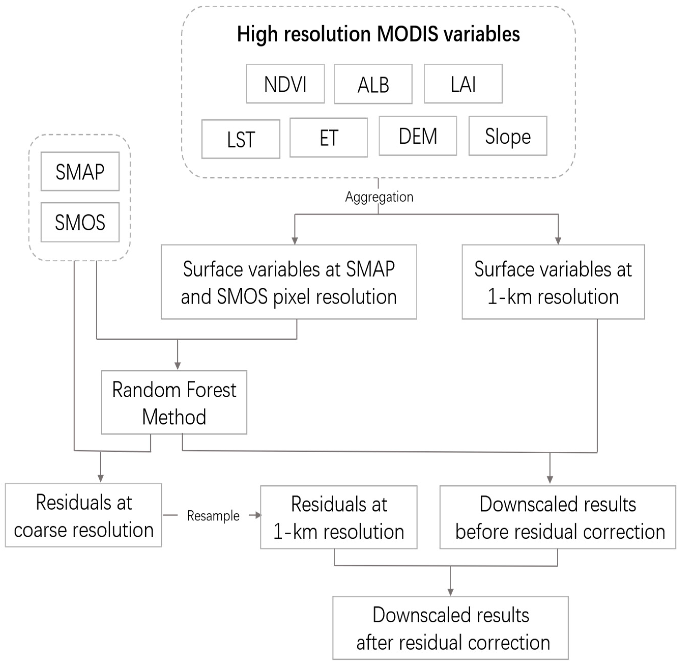
The downscaling process of passive microwave SSM products is shown in Figure 2. The following steps explain the flowchart:
Step 1: The high-resolution MODIS variables and DEM were resampled to the coarse resolution of the SMAP and SMOS SSM data. Then the RF method was used to establish the regression relationship between surface variables and soil moisture products at coarse resolution.
Step 2: The residual error between the RF downscaling prediction results and the original data needs to be calibrated. The residual with coarse resolution was calculated by estimated results which were resampled by bilinear to coarse resolution and the original soil moisture. Then ordinary Kriging interpolation method was used to interpolate the coarse resolution residual to the 1 km.
Step 3: Using the RF regression model established in the first step, the 1 km surface variable was used to obtain the estimated soil moisture with a resolution of 1 km.
Step 4: The estimated soil moisture data of 1 km was added the residual at 1 km to obtain the downscaled results after residual correction.
In the construction of the RF downscaling model, 70%, 15%, and 15% of the data were randomly selected as the training set, verification set, and the testing set, respectively. The quality of the model was evaluated with the testing set after obtaining the optimal model with the minimum RMSE as the standard. Additionally, the SHAP methodology [55,56,57,58] was used here to interpret the relationships of the input surface variables with the model predictions.
3.2. Triple Collocation Error Model
The triple collocation method is based on some assumptions, the most important of which are:
- Linear calibration is sufficient;
- The measurement errors are uncorrelated to each other;
- The measurement errors are constant over the range of measured values.
The error model employed in the triple collocation reads:
where xi stands for a collocated measurement by system i, with I = 0,1,2, t for the signal common to all three systems (sometimes referred to as true signal or truth), ai for the calibration scaling, bi for the calibration bias, and εi for the random error of system i.
The TC method obtains the error εi in (1) by calculating the covariance between systems:
where σt2 stands for variance of the system t. Additionally, the TC problem can be solved under the following assumptions:
- 4.
- Linear calibration is sufficient;
- 5.
- The errors εi in Formula (1) have zero average and variance σi2;
- 6.
- The errors εi are uncorrelated to each other, to the common signal t, and to the calibration parameters.
Therefore, Formula (2) also can be rewritten as follows:
Based on the error model in Equations (1)–(3), we used the equation of covariance notation which proposed by Gruber et al. to calculate the error variance:
where is the variance of the random errors; is the root mean square error of the each of the three data sets.
3.3. TVDI
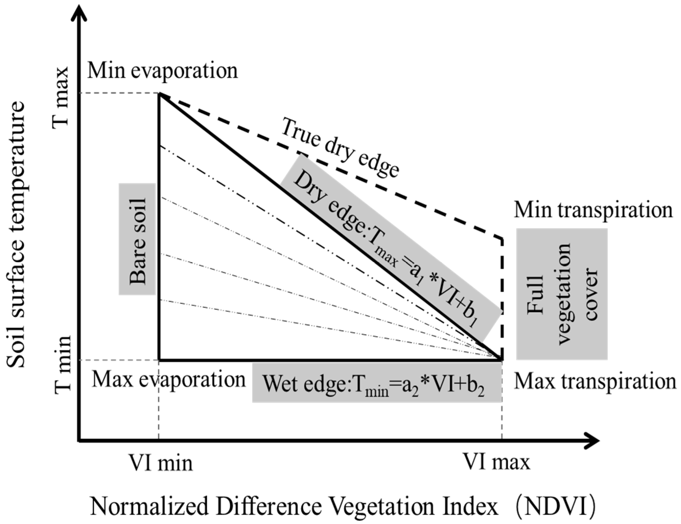
A scatter plot of vegetation index and surface temperature often results in a triangular shape or a trapezoid shape, Sandholt defined a simplified temperature vegetation dryness index (TVDI), in which the ‘wet edge’ is modeled as a horizontal line that parallel to the NDVI axis, and the ‘dry edge’ is modeled as a linear fit to NDVI [59]. Figure 3 shows the conceptual NDVI-Ts space, the highest surface temperature and the lowest surface temperature under the same vegetation index were extracted to fit linearly with vegetation index. Then the dry edge and wet edge equations were calculated for coefficients a and b. TVDI was found can be an index indicating the degree of drought on the ground and can be defined as:
where Ts stands for the regional surface temperature, Ts min stands for the minimum land surface temperature in the triangle, and Ts max stands for the maximum surface temperature observation for a given NDVI.
4. Results
4.1. Prediction Performance Results of the RF Method
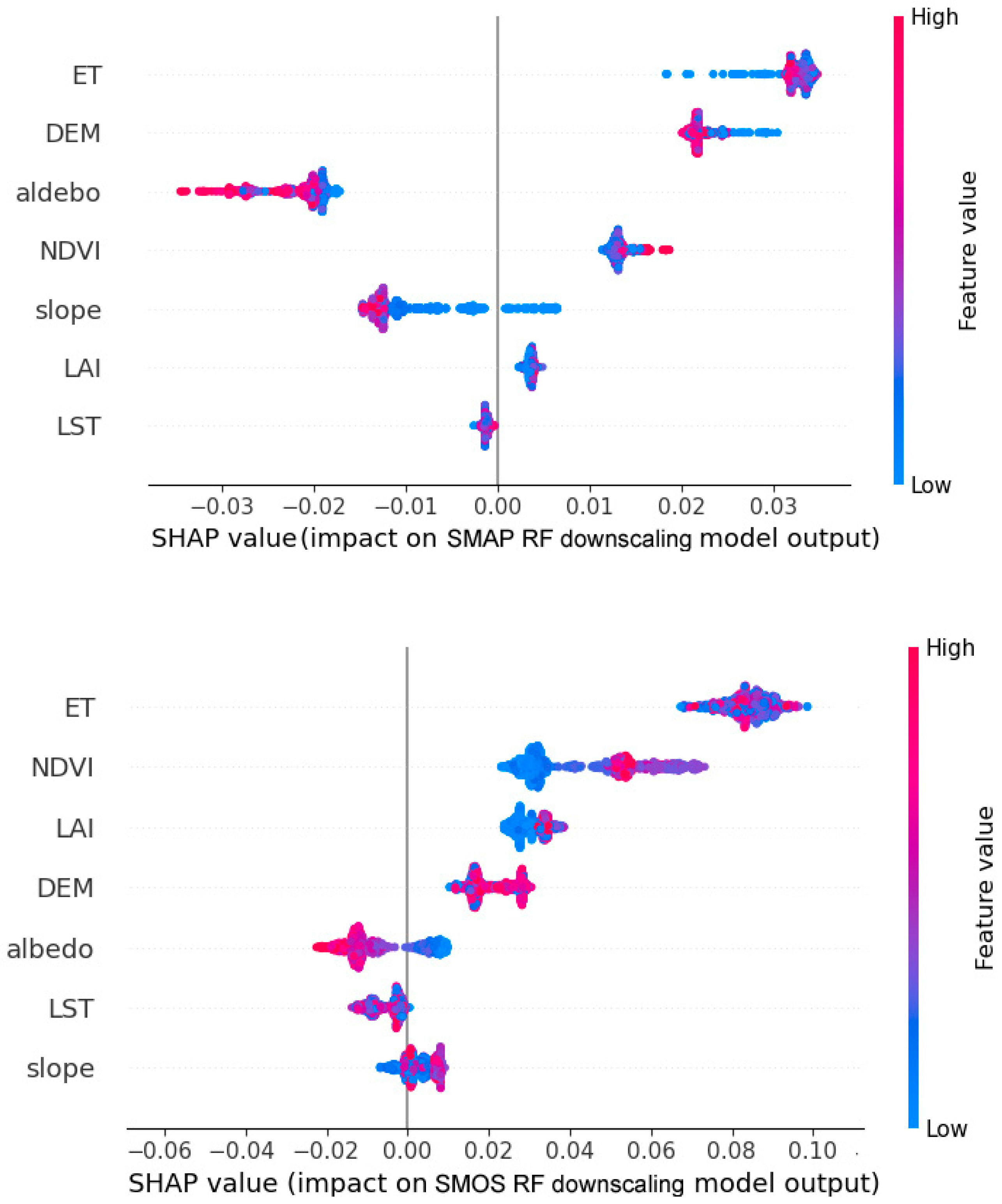
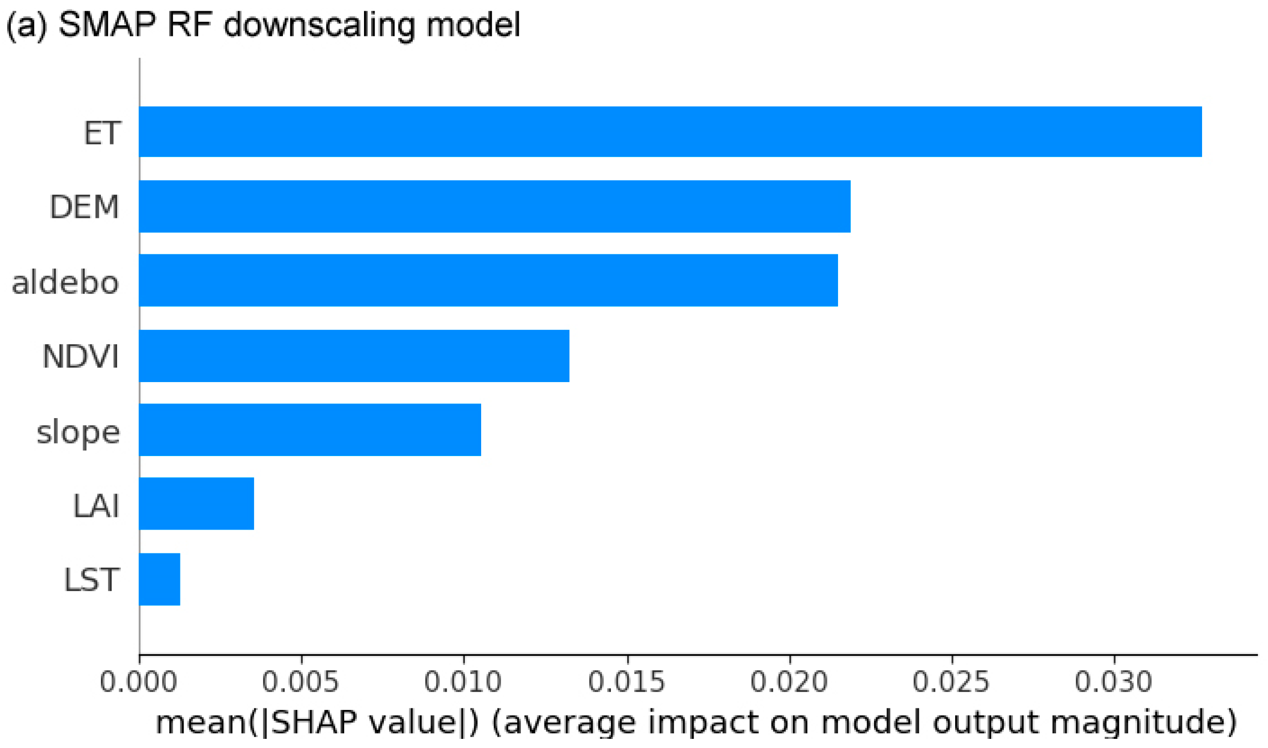
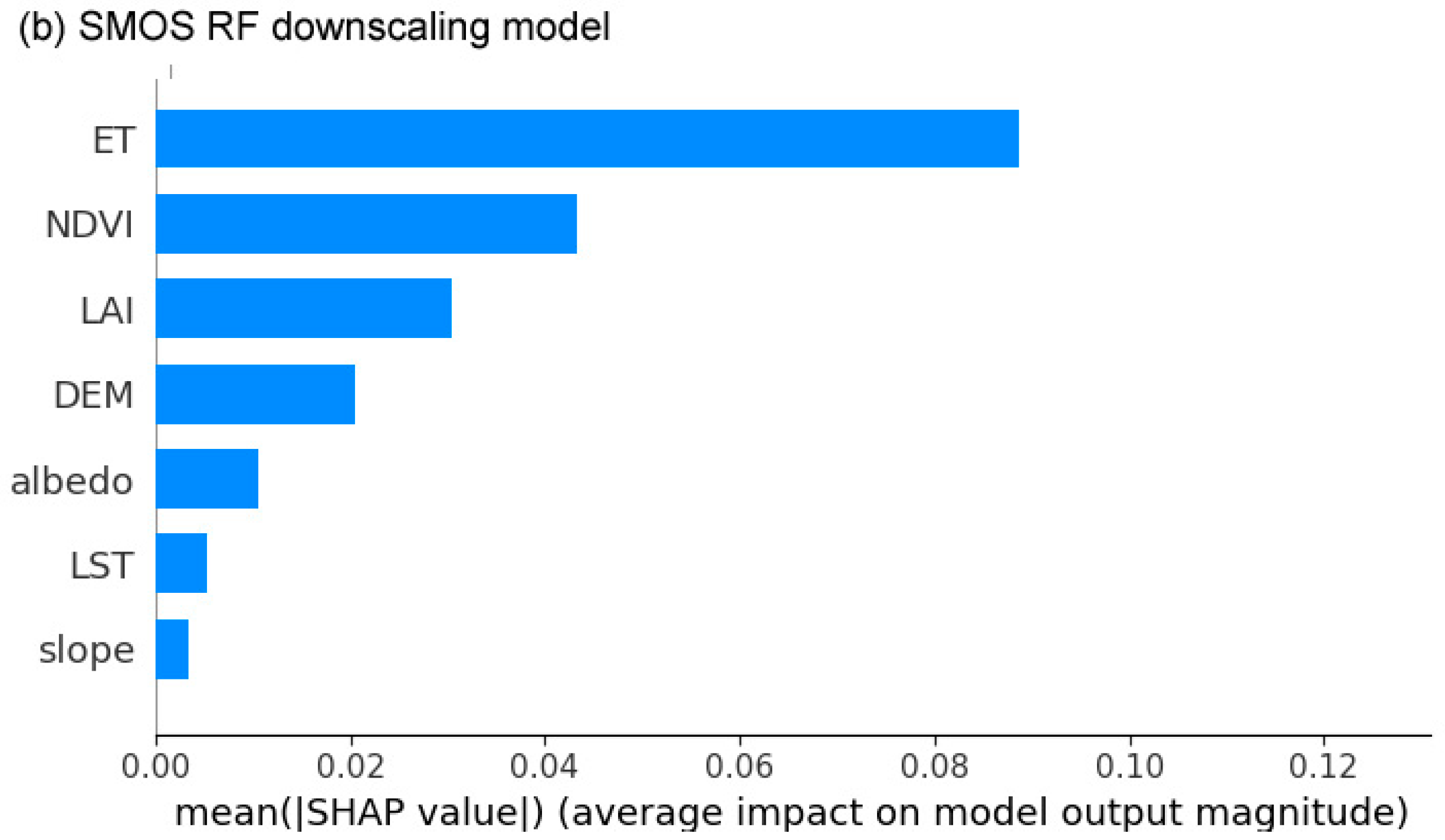
The test accuracy R2 of the RF downscaling model of SMAP and SMOS was 0.763 and 0.644, respectively, and the RMSE was 0.044 and 0.099, respectively. It shows that no over-or underfitting was experienced, and the prediction effects of the RF downscaling models of these two products are well. Figure 4 shows the summary plot of the SHAP values on two RF downscaling models which can interpret the relationships of the input different surface variables with the downscaled prediction results. Each row represents an input variable, and the horizontal axis is the SHAP value. The sign of the SHAP value (positive or negative) indicates the positive or negative correlation, and the larger the value, the more it affects the prediction accuracy. The color scheme represents the importance of the surface variables on predictions from low to high. Figure 4 shows that compared with other surface variables, ET, DEM, and albedo have a greater impact on the SMAP downscaling results, while ET, NDVI, and LAI have a greater impact on SMOS downscaling. The larger the ET value, the greater the impact on the prediction results. For the SMAP downscaling model, higher albedo value and lower DEM have a greater impact on the predicted value. For the SMOS downscaling model, the higher NDVI value obviously affects the prediction results. Figure 5 shows the feature importance plot of the mean SHAP values on RF downscaling model, it takes the average of the absolute value of the SHAP value of each feature as the importance of the feature to obtain a bar graph. It shows that ET is most influences the predicting effects among all variables. LST is the least one that impact the SMAP downscaling model, and slope is the least one that impact the SMOS downscaling model.
4.2. Downscaled Results Based on the RF Method
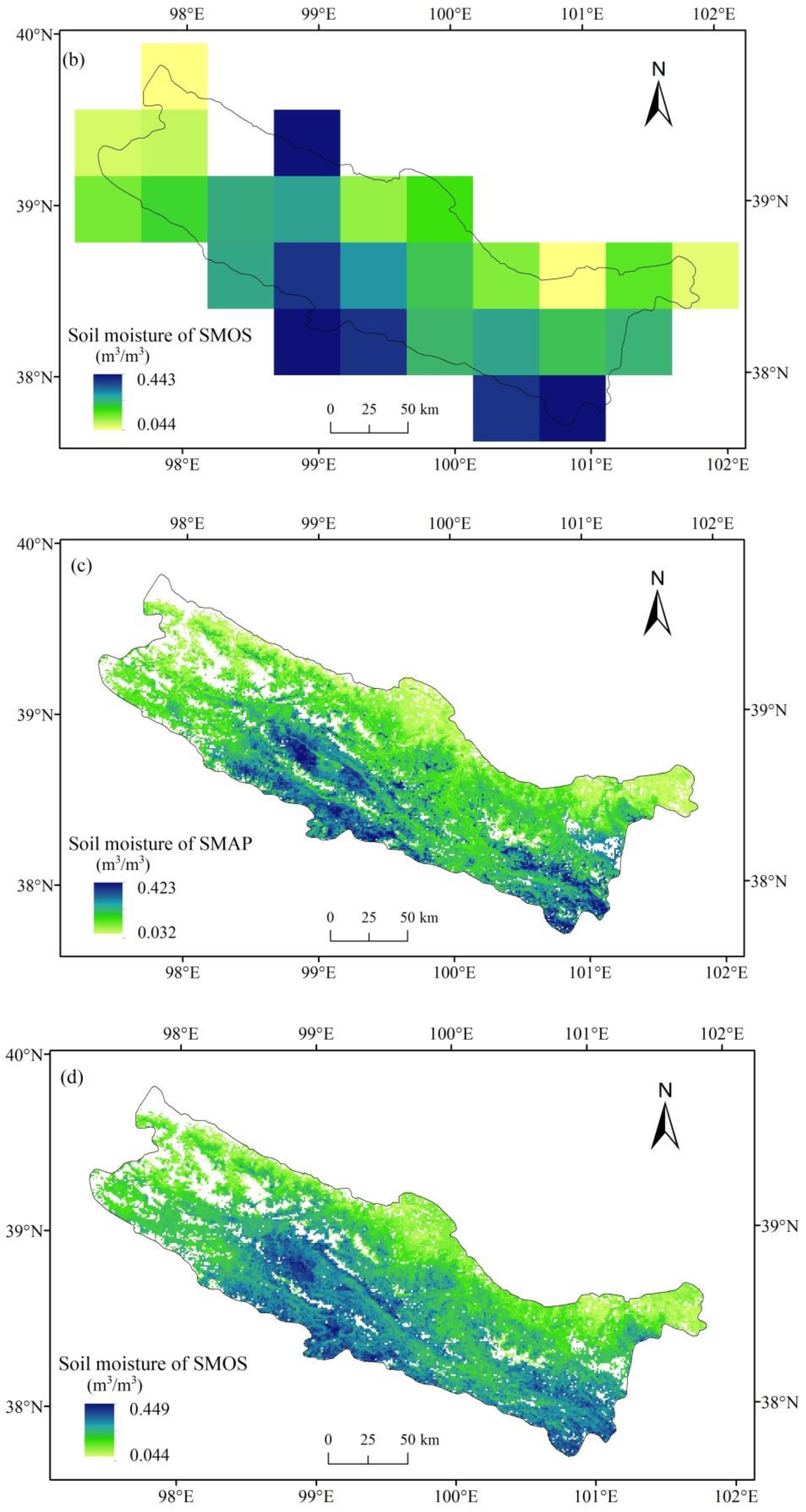
Based on the RF downscaling model constructed at coarse resolution, the soil moisture was estimated at high resolution using MODIS variables with a resolution of 1 km, and then the coarse resolution residuals were resampled to the residuals at 1 km while bilinear interpolation was used. Next, the estimated downscaled results at 1 km were added to the residual at 1 km to obtain high resolution microwave soil moisture after residual correction was applied. Figure 6a–d show the original soil moisture data at coarse resolution and the final downscaled results after residual correction of two products, respectively. Figure 6 shows that the two original soil moisture are consistent with the trend of the estimated soil moisture after applying a residual correction, which indicates that the RF method-based downscaling method is well applicable to the study area.
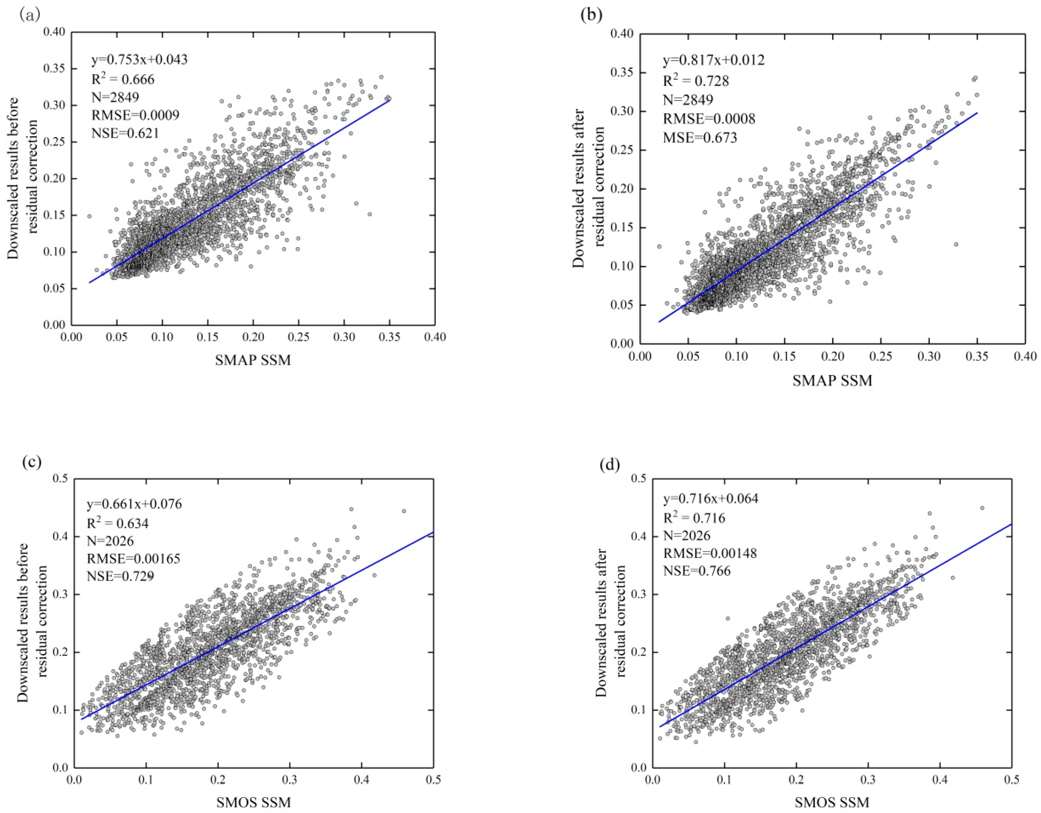
The scatter plots of the downscaled SSM results and original SSM in 2015 are presented in Figure 7. Figure 7a,b are the scatter plots of the SMAP downscaled results before and after the residual correction, respectively. Similarly, Figure 7c,d are the scatter plots of downscaled SMOS results. It can be seen from the figure that the data points of SMAP are more scattered than that of SMOS, but in general both are very concentrated. The R2 values of the downscaled results of SMAP and SMOS with the original data before residual correction are 0.67 and 0.63, respectively. After applying residual correction, R2 values increased to 0.73 and 0.72 respectively. In general, the downscaled results of SMAP are closer to the original values than SMOS. The results indicate that the downscaling model has good applicability in the Heihe River Basin.
4.3. Validation with the In Situ SSM Measurements of Babaohe River Basin
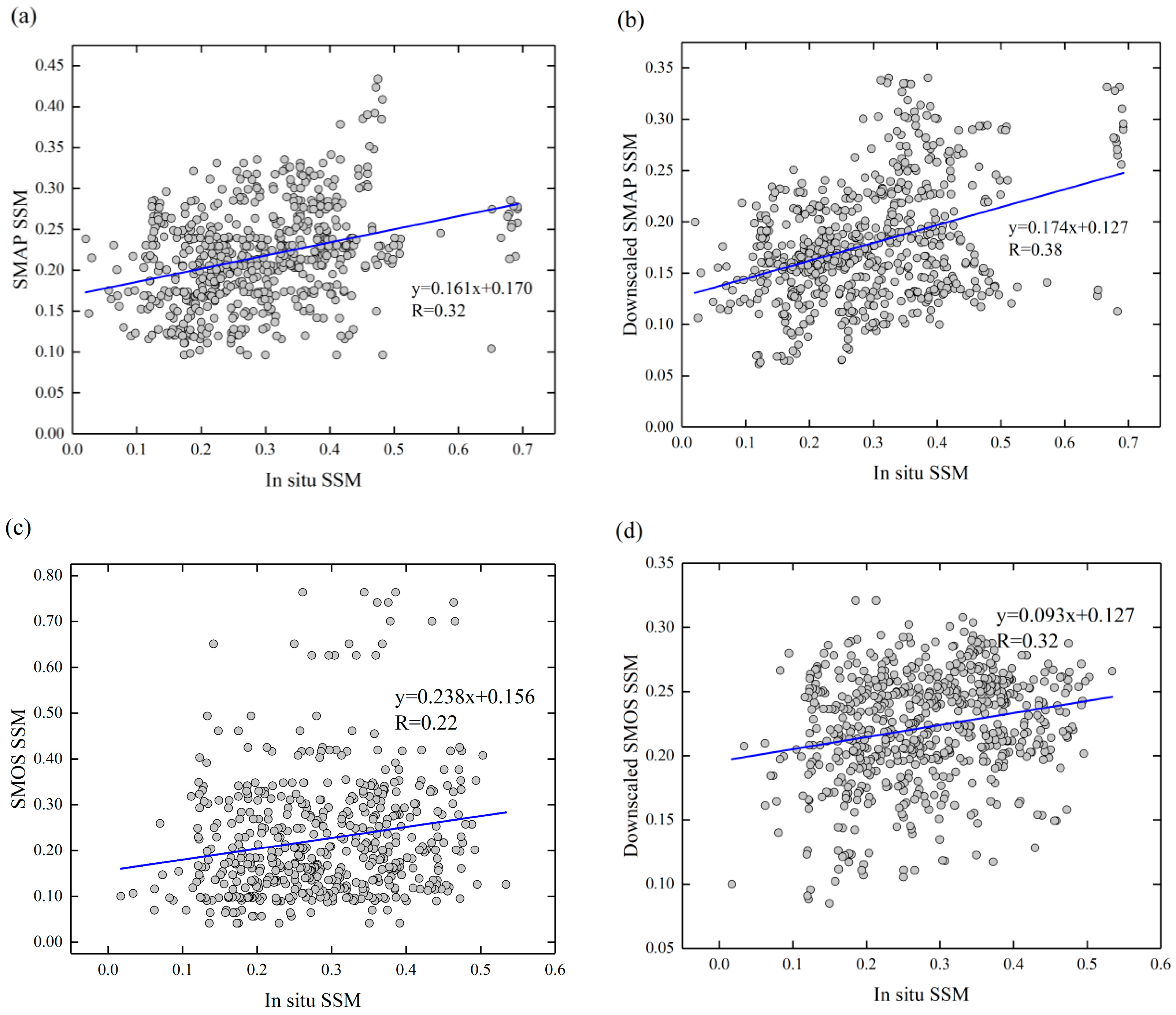
In situ soil moisture is used to verify the accuracy of remote sensing products with different resolutions will cause different errors, which cannot be ignored [46]. Therefore the results of validation with the in situ SSM measurements of the original SSM data and their corresponding downscaled SSM which was resampled to the original grid scale are shown in Figure 8. The results show the correlation coefficient R values between the original SMAP and SMOS and in situ SSM are 0.32 and 0.22 respectively. Furthermore, the results show that the R values between the downscaled results based on RF and the in situ soil moisture are 0.38 and 0.32 respectively. Regarding the performance of the downscaled SSM data, an obvious improvement in R of both two products is found when compared with the validation for the coarse resolution data. In general, whether it is before or after downscaling, the correlation between SMAP SSM and in situ SSM is much better than SMOS in grid-scale. Additionally, the scatter plots of SMAP and in situ SSM are more scattered than SMOS, indicating that the SMAP SSM is closer to the in situ SSM.
In addition, the annual changes of SMAP and SMOS SSM in 2015 are compared with in situ SSM of the Babaohe River basin are shown in Figure 9. In general, SMAP is more able to reflect the temporal change trend of in situ soil moisture than SMOS, and they are all lower than the observed data (dryness). The details of the two products’ differences at basin scale are shown in Table 2. The R value is 0.31 and 0.24 for the original SMAP and SMOS products, respectively, indicating that R2 of the two original products and in situ SSM are both low but the SMAP SSM performed a little better. The RMSE values are 0.139 m3/m3 and 0.207 m3/m3 for the original SMAP and SMOS products, indicating the accuracy of SMAP products is higher than that of SMOS, but in general, both are relatively low. After downscaling, the R values are 0.56 and 0.32 for the downscaled SMAP and SMOS, respectively, indicating that the R values of the two products have improved significantly and the downscaled SMAP products still have a better trend fitting effect on observation data. Additionally, both the RMSE, bias and ubRMSE values have decreased, indicating that the accuracy of the two downscaled products has been improved. The ubRMSE value of the downscaled SMAP is 0.028 m3/m3, which is far beyond the accuracy of 0.040 m3/m3, indicating the accuracy of the downscaled SMAP SSM is very well at the Babao River Basin scale.
4.4. Validation with the TC Model in Upstream of the Heihe River Basin
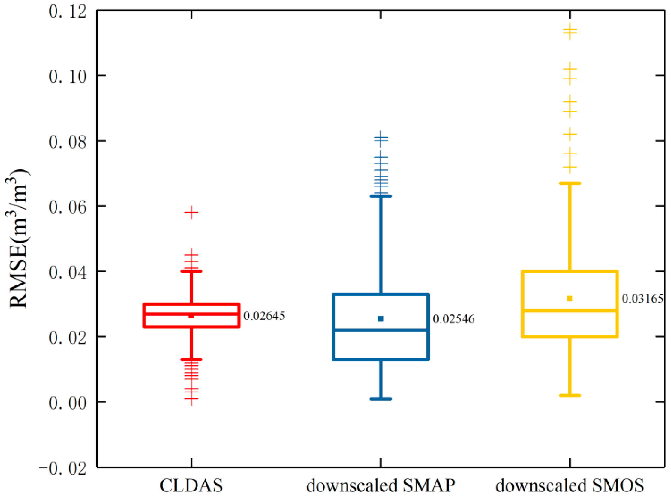
The verification results based on the in situ measurements cannot represent the entire upstream of the Heihe River Basin. By using the TC method, the RMSE for the three data sets which are CLDAS SSM, downscaled results of SMAP and SMOS in the upstream of the Heihe River Basin from 2015 to 2017 were calculated and shown in Figure 10, and Figure 11 shows the error statistics of the three data sets.
As shown in Figure 10, the data quality of CLDAS and downscaled SMAP is better and the RMSE of SMOS data is the largest, indicating that uncertainty of the downscaled SMOS is the highest. The high RMSE values areas of downscaled SMAP and SMOS are located in the central area of the south, because alpine deserts and alpine meadows are mostly distributed in this part of the area, remote sensing observation signals are often doped with high noise here. As shown in Figure 11, the average RMSE value of the three data sets of CLDAS, downscaled SMAP and downscaled SMOS in the spatial range are 0.0265, 0.0255 and 0.0317 m3/m3, respectively. It can be seen from the boxplots that the RMSE values of CLDAS are relatively concentrated, and the abnormal values of downscaled SMOS are more and large. The upper (75%) and the lower quartile (25%) of CLDAS and the downscaled SMAP are approximately between 0.01~0.04 m3/m3, indicating that most of the values of these two data sets can meet the accuracy requirements proposed by the Global Climate Observation System (GCOS), which requires the RMSE between the soil volumetric water content of remote sensing and in situ measurement is less than 0.04 m3/m3. The average and median RMSE values of downscaled SMAP data are the smallest, and there are fewer outliers, indicating that the data has less dispersion and better stability.
4.5. Validation with the Trend Analysis of TVDI in Upstream of the Heihe River Basin
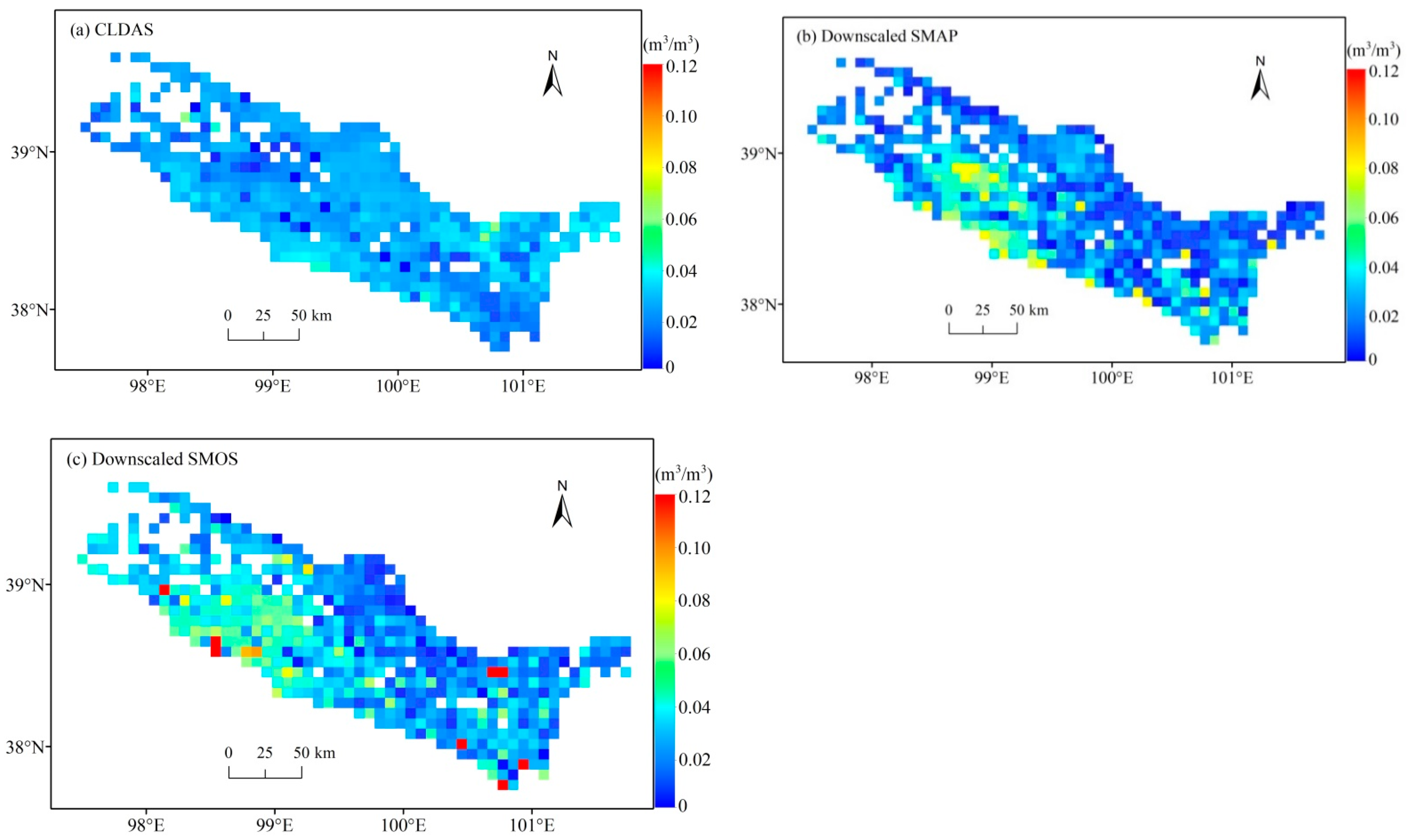
The distribution of TVDI which is an indicator to verify the trend of downscaled results of the upstream of the Heihe River Basin on 31 July 2015 is shown in Figure 12, and the date is consistent with Figure 6 for comparison. The area with a smaller TVDI value proves that the drought degree is lower; conversely, the area with a larger TVDI value has a higher drought degree.
The comparison of the trend distribution of these three figures can intuitively show that the trend distribution in the upstream of the Heihe River Basin of downscaled results of SMAP and SMOS soil moisture are consistent with the degree of drought reflected by TVDI, and they all show higher soil moisture in the middle area of the southern part of the study area, while the soil moisture in the strip-shaped regions along the boundary of the study area in the northwest and north is low. However, the SMOS downscaled results show that the high-value areas of soil moisture in the south are continuously distributed, which is consistent with the degree of drought in the south reflected by TVDI, while the SMAP downscaled results shows that the high-value areas of soil moisture in the south are discontinuous. Therefore, the soil moisture distribution shown by the SMOS downscaled results is closer to the drought degree reflected by TVDI.
The TVDI is divided into 5 levels, which are extremely humid (0 < TVDI < 0.2), humid (0.2 < TVDI < 0.4), normal (0.4 < TVDI < 0.6), drought (0.6 < TVDI < 0.8) and extremely drought (0.8 < TVDI < 1). The statistical information of soil moisture at all levels of the three figures is shown in Figure 13. It can be seen from it that as the TVDI increases, the two downscaled soil moisture results are both decrease, negatively correlated with TVDI, which is consistent with the concept of TVDI. The correlation analysis between the two downscaled products and TVDI shows that the correlation coefficient of downscaled SMOS is higher than that of SMAP, indicating that the soil moisture trend of downscaled SMOS is closer to the degree of drought reflected by TVDI. In each level of soil moisture, the median, average and other statistical information of SMOS are higher than SMAP, indicating that the soil moisture values of downscaled SMOS are generally higher than the results of downscaled SMAP. At the same time, we found that the corresponding soil moisture data of the two downscaled products are similar when the TVDI is extremely humid and humid, indicating that the degree of soil moisture in the study area is the same when 0 < TVDI < 0.4.
5. Discussion
The TC method is used in this paper to analyze the errors of three data sets: downscaled SMAP, downscaled SMOS and CLDAS. One of the TC analysis assumptions is that the error of the three datasets should be independent of each other. The error relationship between these data sets can be called error-cross-correction (ECC) [60]. In this article and past studies, ECC was typically assumed to be zero between all data sets [61]. However, recent works have revealed the presence of non-zero ECC between active and passive soil moisture retrievals [62,63]. The EEC of SMAP-SMOS in this article is actually impossible to be zero because they are both from the L-band observation. Therefore, it is more prudent to check the ECC levels in SMAP-SMOS soil moisture data used in this article, these issues will be further analyzed in future work.
6. Conclusions
In previous studies in situ SSM measurements were used to verify coarse-resolution microwaves remote sensing products. Here, downscaled products with high-resolution help reduce this error of validation caused by scale difference. In this paper, the performance of two passive microwave downscaled SSM products were compared and analyzed for capturing SSM information in upstream of the Heihe River Basin. RF method is proposed for downscaling original coarse-resolution SSM products using remote sensing data from Optical/TIR observations. The results showed the ET has a greater impact on RF downscaling model and RF downscaling method is strongly applicable in the study area. The downscaled results of two products after a residual correction have more details and are more representative of the spatial distribution of soil moisture. The validation with the in situ SSM measurements indicates the correlation between downscaled SMAP and in situ SSM is better than downscaled SMOS in Babaohe River Basin. Selected CLDAS SSM data as the true signal, the accuracy of the CLDAS, downscaled SMAP and downscaled SMOS of the Heihe River Basin were calculated and compared using the Triple Collocation method. The results showed that the RMSEs of the three data sets were 0.0265, 0.0255 and 0.0317, indicating downscaled SMAP has smaller errors in the Heihe River Basin than others. Additionally, the soil moisture distribution in the study area shown by the SMOS downscaled results is closer than downscaled SMAP to the degree of drought reflected by TVDI.
In general, the downscaled SMAP SSM performed better than the downscaled SMOS in the upstream of the Heihe River Basin. The downscaled results not only show better spatial heterogeneity but also present good temporal consistency in terms of time series SSM from in situ measurement, it provides higher resolution and more accurate data support for subsequent soil moisture research in the Heihe River Basin.
Author Contributions
Conceptualization, Y.W.; methodology, Y.W. and G.Z.; software, Y.W. and R.X.; validation, Y.W. and J.Z.; formal analysis, Y.W. and G.Z.; investigation, resources, data curation, writing—original draft preparation, Y.W.; writing—review and editing, J.Z.; visualization Y.W. and J.Y.; supervision, J.Z.; project administration, funding acquisition, J.Z. All authors have read and agreed to the published version of the manuscript.
Funding
This research was funded by National Natural Science Foundation of China (No. 41661084) and Northwest Normal University Excellent Doctoral Dissertation Cultivation Funding Project.
Institutional Review Board Statement
Not applicable.
Informed Consent Statement
Not applicable.
Data Availability Statement
The data used in this manuscript are available by writing to the first author.
Acknowledgments
We acknowledge the data providers in Heihe Eco-hydrological Remote Sensing Experiment. We appreciate constructive comments and suggestions from Lichang Yin in the machine learning code.
Conflicts of Interest
The authors declare no conflict of interest.
Abbreviations
Commonly used abbreviations in the paper:
| SSM | Surface soil moisture |
| RF | Random forest |
| SMAP | Soil Moisture Active Passive Mission |
| SMOS | Soil Moisture and Ocean salinity |
| TC | Triple Collocation |
| TVDI | Temperature Vegetation Dryness Index |
| RMSE | Root square error |
| AMSR-E | Advanced Microwave Scanning Radiometer |
| AMSR-2 | Advanced Microwave Scanning Radiometer-2 |
| FY | Feng Yun |
| LST | Land Surface Temerature |
| GWR | Geographically Weighted Regression |
| MODIS | Moderate-Resolution Imaging Spectroradiometer |
| OLS | Ordinary Least Square |
| HIWATER | Heihe Watershed Allied Telemetry Experimental Research |
| CLDAS CMA | Land Data Assimilation System |
| LAI | Leaf area index |
| ALB | albedo |
| ET | evapotranspiration |
| NDVI | Normalized Difference Vegetation Index |
| DEM | Digital elevation model |
References
- Chen, S.; She, D.; Zhang, L.; Guo, M.; Liu, X. Spatial downscaling methods of soil moisture based on multisource remote sensing data and its application. Water 2019, 11, 1401. [Google Scholar] [CrossRef] [Green Version]
- Mao, Y.; Crow, W.T.; Nijssen, B. Dual state/rainfall correction via soil moisture assimilation for improved streamflow simulation: Evaluation of a large-scale implementation with Soil Moisture Active Passive (SMAP) satellite data. Hydrol. Earth Syst. Sci. 2020, 24, 615–631. [Google Scholar] [CrossRef] [Green Version]
- McColl, K.A.; Alemohammad, S.H.; Akbar, R.; Konings, A.G.; Yueh, S.; Entekhabi, D. The global distribution and dynamics of surface soil moisture. Nat. Geosci. 2017, 10, 100–104. [Google Scholar] [CrossRef]
- Seneviratne, S.I.; Corti, T.; Davin, E.L.; Hirschi, M.; Jaeger, E.B.; Lehner, I.; Orlowsky, B.; Teuling, A.J. Investigating soil moisture-climate interactions in a changing climate: A review. Earth-Sci. Rev. 2010, 99, 125–161. [Google Scholar] [CrossRef]
- Luca, B.; Angelica, T.; Paolo, F.; Wouter, D.; Felix, Z.; Alexander, G.; Diego, F.P. How much water is used for irrigation? A new approach exploiting coarse resolution satellite soil moisture products. Int. J. Appl. Earth Obs. Geoinf. 2018, 73, 752–766. [Google Scholar] [CrossRef]
- Hagan, D.F.T.; Wang, G.; Liang, X.S.; Dolman, H.A.J. A time-varying causality formalism based on the liang-kleeman information flow for analyzing directed interactions in nonstationary climate systems. J. Clim. 2019, 32, 7521–7537. [Google Scholar] [CrossRef]
- Jalilvand, E.; Tajrishy, M.; Brocca, L.; Massari, C.; Ghazi Zadeh Hashemi, S.A.; Ciabatta, L. Estimating the drainage rate from surface soil moisture drydowns: Application of DfD model to in situ soil moisture data. J. Hydrol. 2018, 565, 489–501. [Google Scholar] [CrossRef]
- Kim, H.; Parinussa, R.; Konings, A.G.; Wagner, W.; Cosh, M.H.; Lakshmi, V.; Zohaib, M.; Choi, M. Global-scale assessment and combination of SMAP with ASCAT (active) and AMSR2 (passive) soil moisture products. Remote Sens. Environ. 2018, 204, 260–275. [Google Scholar] [CrossRef]
- Vogel, M.; Zscheischler, J.; Seneviratne, S. Varying soil moisture-atmosphere feedbacks explain divergent temperature extremes and precipitation projections in Central Europe. Earth Syst. Dyn. 2018, 9, 1107–1125. [Google Scholar] [CrossRef] [Green Version]
- Kim, S.; Zhang, R.; Pham, H.; Sharma, A. A review of satellite-derived soil moisture and its usage for flood estimation. Remote Sens. Earth Syst. Sci. 2019, 2, 225–246. [Google Scholar] [CrossRef]
- Tian, S.; Tregoning, P.; Renzullo, L.J.; Dijk, A.V.; Walker, J.P.; Pauwels, V.; Allgeyer, S. Improved water balance component estimates through joint assimilation of GRACE water storage and SMOS soil moisture retrievals. Water Resour. Res. 2017, 53, 1820–1840. [Google Scholar] [CrossRef]
- Dorigo, W.A.; Wagner, W.; Hohensinn, R.; Hahn, S.; Paulik, C.; Xaver, A.; Gruber, A.; Drusch, M.; Mecklenburg, S.; Vanch, M. The international soil moisture network: A data hosting facility for global in situ soil moisture measurements. Hydrol. Earth Syst. Sci. 2011, 15, 1675–1698. [Google Scholar] [CrossRef] [Green Version]
- Zreda, M.; Shuttleworth, W.J.; Zeng, X.; Zweck, C.; Desilets, D.; Franz, T.; Rosolem, R. Cosmos: The cosmic-ray soil moisture observing system. Hydrol. Earth Syst. Sci. 2012, 16, 4079–4099. [Google Scholar] [CrossRef] [Green Version]
- Gelaro, R.; Mccarty, W.; Suárez, M.J.; Todling, R.; Zhao, B. The modern-era retrospective analysis for research and applications, version 2 (MERRA-2). J. Clim. 2017, 30, 5419–5454. [Google Scholar] [CrossRef] [PubMed]
- Wigneron, J.P.; Li, X.; Frappart, F.; Fan, L.; Moisy, C. SMOS-IC data record of soil moisture and L-VOD: Historical development, applications and perspectives. Remote Sens. Environ. 2021, 254, 112–238. [Google Scholar] [CrossRef]
- Parinussa, R.M.; De Jeu, R.A.M.; Van der Schalie, R.; Crow, W.T.; Lei, F.; Holmes, T.R.H. A Quasi-Global Approach to Improve Day-Time Satellite Surface Soil Moisture Anomalies through the Land Surface Temperature Input. Climate 2016, 4, 50. [Google Scholar] [CrossRef] [Green Version]
- Zawadzki, J.; Kędzior, M. Soil moisture variability over Odra watershed: Comparison between SMOS and GLDAS data. Int. J. Appl. Earth Obs. Geoinf. 2016, 45, 110–124. [Google Scholar] [CrossRef]
- Kędzior, M.; Zawadzki, J. Comparative study of soil moisture estimations from SMOS satellite mission, GLDAS database, and cosmic-ray neutrons measurements at COSMOS station in Eastern Poland. Geoderma 2016, 283, 21–31. [Google Scholar] [CrossRef]
- Piles, M.; Sánchez, N.; Vall-Llossera, M.; Camps, A.; Martínez-Fernandez, J.; Martinez, J.; Gonzalez-Gambau, V. A downscaling approach for SMOS land observations: Evaluation of high-resolution soil moisture maps over the Iberian peninsula. IEEE J. Sel. Top. Appl. Earth Obs. Remote Sens. 2014, 7, 3845–3857. [Google Scholar] [CrossRef] [Green Version]
- Entekhabi, D.; Njoku, E.G.; O’Neill, P.E.; Kellogg, K.H.; Crow, W.T.; Edelstein, W.N.; Entin, J.K.; Goodman, S.D.; Jackson, T.J.; Johnson, J.; et al. The Soil Moisture Active Passive (SMAP) Mission. Proc. IEEE 2010, 98, 704–716. [Google Scholar] [CrossRef]
- Tagesson, T.; Horion, S.; Nieto, H.; Zaldo Fornies, V.; Mendiguren González, G.; Bulgin, C.E.; Ghent, D.; Fensholt, R. Disaggregation of SMOS soil moisture over West Africa using the Temperature and Vegetation Dryness Index based on SEVIRI land surface parameters. Remote Sens. Environ. 2018, 206, 424–441. [Google Scholar] [CrossRef] [Green Version]
- Usowicz, B.; Marczewski, W.; Usowicz, J.B.; Łukowski, M.I.; Lipiec, J. Comparison of surface soil moisture from SMOS satellite and ground measurements. Int. Agrophysics 2014, 28, 359–369. [Google Scholar] [CrossRef] [Green Version]
- Sridhar, V.; Jaksa, W.T.A.; Fang, B.; Lakshmi, V.; Hubbard, K.G.; Jin, X. Evaluating Bias-Corrected AMSR-E Soil Moisture Using In Situ Observations and Model Estimates. Vadose Zo. J. 2013, 12, 1–13. [Google Scholar] [CrossRef]
- Abbaszadeh, P.; Moradkhani, H.; Zhan, X. Downscaling SMAP Radiometer Soil Moisture Over the CONUS Using an Ensemble Learning Method. Water Resour. Res. 2019, 55, 324–344. [Google Scholar] [CrossRef] [Green Version]
- Das, N.N.; Entekhabi, D.; Dunbar, R.S.; Colliander, A.; Chen, F.; Crow, W.; Jackson, T.J.; Berg, A.; Bosch, D.D.; Caldwell, T.; et al. The SMAP mission combined active-passive soil moisture product at 9 km and 3 km spatial resolutions. Remote Sens. Environ. 2018, 211, 204–217. [Google Scholar] [CrossRef]
- Colliander, A.; Jackson, T.J.; Chan, S.K.; O’Neill, P.; Bindlish, R.; Cosh, M.H.; Caldwell, T.; Walker, J.P.; Berg, A.; McNairn, H.; et al. An assessment of the differences between spatial resolution and grid size for the SMAP enhanced soil moisture product over homogeneous sites. Remote Sens. Environ. 2018, 207, 65–70. [Google Scholar] [CrossRef]
- Parinussa, R.M.; Holmes, T.R.H.; Wanders, N.; Dorigo, W.A.; De Jeu, R.A.M. A preliminary study toward consistent soil moisture from AMSR2. J. Hydrometeorol. 2015, 16, 932–947. [Google Scholar] [CrossRef]
- Park, S.; Park, S.; Im, J.; Rhee, J.; Shin, J.; Park, J.D. Downscaling GLDAS Soil moisture data in East Asia through fusion of Multi-Sensors by optimizing modified regression trees. Water 2017, 9, 332. [Google Scholar] [CrossRef] [Green Version]
- Al-Jassar, H.K.; Rao, K.S. Monitoring of soil moisture over the Kuwait desert using remote sensing techniques. Int. J. Remote Sens. 2010, 31, 4373–4385. [Google Scholar] [CrossRef]
- Zhao, W.; Sánchez, N.; Lu, H.; Li, A. A spatial downscaling approach for the SMAP passive surface soil moisture product using random forest regression. J. Hydrol. 2018, 563, 1009–1024. [Google Scholar] [CrossRef]
- Chauhan, N.S.; Miller, S.; Ardanuy, P. Spaceborne soil moisture estimation at high resolution: A microwave-optical/IR synergistic approach. Int. J. Remote Sens. 2003, 24, 4599–4622. [Google Scholar] [CrossRef]
- Choi, M.; Hur, Y. A microwave-optical/infrared disaggregation for improving spatial representation of soil moisture using AMSR-E and MODIS products. Remote Sens. Environ. 2012, 124, 259–269. [Google Scholar] [CrossRef]
- Xu, S.; Wu, C.; Wang, L.; Gonsamo, A.; Shen, Y.; Niu, Z. A new satellite-based monthly precipitation downscaling algorithm with non-stationary relationship between precipitation and land surface characteristics. Remote Sens. Environ. 2015, 162, 119–140. [Google Scholar] [CrossRef]
- Zhan, C.; Han, J.; Hu, S.; Liu, L.; Dong, Y. Spatial Downscaling of GPM Annual and Monthly Precipitation Using Regression-Based Algorithms in a Mountainous Area. Adv. Meteorol. 2018, 2018, 1506017. [Google Scholar] [CrossRef] [Green Version]
- Brunsdon, C.; Fotheringham, A.S.; Charlton, M.E. Geographically weighted regression: A method for exploring spatial nonstationarity. Geogr. Anal. 1996, 28, 281–298. [Google Scholar] [CrossRef]
- Breiman, L. Random forests. Mach. Learn. 2001, 45, 5–32. [Google Scholar] [CrossRef] [Green Version]
- Im, J.; Park, S.; Rhee, J.; Baik, J.; Choi, M. Downscaling of AMSR-E soil moisture with MODIS products using machine learning approaches. Environ. Earth Sci. 2016, 75, 1120. [Google Scholar] [CrossRef]
- Park, S.; Im, J.; Park, S.; Rhee, J. AMSR2 soil moisture downscaling using multisensor products through machine learning approach. Int. Geosci. Remote Sens. Symp. 2015, 201, 1984–1987. [Google Scholar] [CrossRef]
- Stoffelen, A. Toward the true near-surface wind speed: Error modeling and calibration using triple collocation. J. Geophys. Res. Ocean. 1998, 103, 7755–7766. [Google Scholar] [CrossRef]
- Yuan, Q.; Xu, H.; Li, T.; Shen, H.; Zhang, L. Estimating surface soil moisture from satellite observations using a generalized regression neural network trained on sparse ground-based measurements in the continental U.S. J. Hydrol. 2020, 580, 124351. [Google Scholar] [CrossRef]
- Gruber, A.; Dorigo, W.A.; Zwieback, S.; Xaver, A.; Wagner, W. Characterizing Coarse-Scale Representativeness of in situ Soil Moisture Measurements from the International Soil Moisture Network. Vadose Zo. J. 2013, 12, vzj2012.0170. [Google Scholar] [CrossRef] [Green Version]
- Draper, C.; Reichle, R.; de Jeu, R.; Naeimi, V.; Parinussa, R.; Wagner, W. Estimating root mean square errors in remotely sensed soil moisture over continental scale domains. Remote Sens. Environ. 2013, 137, 288–298. [Google Scholar] [CrossRef] [Green Version]
- Zhang, L.; He, C.; Li, J.; Wang, Y.; Wang, Z. Comparison of IDW and Physically Based IDEW Method in Hydrological Modelling for a Large Mountainous Watershed, Northwest China. River Res. Appl. 2017, 33, 912–924. [Google Scholar] [CrossRef]
- Li, X.; Liu, S.; Ma, M.; Xiao, Q.; Liu, Q.; Jin, R.; Che, T.; Wang, W.; Qi, Y.; Li, H.; et al. HiWATER: An integrated remote sensing experiment on hydrological and ecological processes in the Heihe River Basin. Adv. Earth Sci. 2012, 27, 481–498. [Google Scholar] [CrossRef]
- Jin, R.; Li, X.; Yan, B.; Luo, W.; Li, X.; Guo, J.; Ma, M.; Kang, J.; Zhang, Y. In troduction of eco-hydrological wireless sensor network in the Heihe River BasinScience. Adv. Earth Sci. 2012, 27, 993–1005. [Google Scholar] [CrossRef]
- Li, X.; Jin, R.; Liu, S.; Ge, Y.; Xiao, Q.; Liu, Q.; Ma, M.; Ran, Y. Upscaling research in HiWATER: Progress and prospects. J. Remote Sens. 2016, 20, 921–932. [Google Scholar] [CrossRef]
- Jin, R.; Kang, J.; Li, X.; Ma, M. HiWATER: WATERNET observation dataset in the upper reaches of the Heihe River Basin in 2015 Monitoring. Natl. Tibet. Plateau Data Cent. 2016. [Google Scholar] [CrossRef]
- Entekhabi, D.; Entekhabi, D.; Yueh, S.; O’Neill, P.; Kellogg, K.; Allen, A.; Bindlish, R.; Brown, M.; Chan, S.; Colliander, A.; et al. SMAP Handbook–Soil Moisture Active Passive: Mapping Soil Moisture and Freeze/Thaw from Space; JPL Publication: Pasadena, CA, USA, 2014. [Google Scholar]
- Entekhabi, D.; Njoku, E.; O’Neill, P.; Spencer, M.; Jackson, T.; Entin, J.; Im, E.; Kellogg, K. The soil moisture active/passive mission (SMAP). Int. Geosci. Remote Sens. Symp. 2008, 3, 3–6. [Google Scholar]
- O’Neill, P.; Chan, S.; Bindlish, R.; Jackson, T.; Colliander, A.; Dunbar, S.; Chen, F.; Piepmeier, J.; Yueh, S.; Entekhabi, D.; et al. Assessment of version 4 of the SMAP passive soil moisture standard product. Int. Geosci. Remote Sens. Symp. 2017, 7, 3941–3944. [Google Scholar] [CrossRef] [Green Version]
- Kerr, Y.H.; Waldteufel, P.; Wigneron, J.P.; Martinuzzi, J.M.; Berger, M. Soil moisture retrieval from space: The soil moisture and ocean salinity (smos) mission. IEEE Trans. Geosci. Electron. 2002, 39, 1729–1735. [Google Scholar] [CrossRef]
- Dandridge, C.; Fang, B.; Lakshmi, V. Downscaling of SMAP Soil Moisture in the Lower Mekong River Basin. Water 2020, 12, 56. [Google Scholar] [CrossRef] [Green Version]
- Yishay, M.; Mariano, S. Learning with Maximum-Entropy Distributions. Mach. Learn. 2001, 45, 123–145. [Google Scholar]
- Bai, J.; Cui, Q.; Zhang, W.; Meng, L. An approach for downscaling SMAP soil moisture by combining Sentinel-1 SAR and MODIS data. Remote Sens. 2019, 11, 2736. [Google Scholar] [CrossRef] [Green Version]
- Can, R.; Kocaman, S.; Gokceoglu, C. A comprehensive assessment of XGBoost algorithm for landslide susceptibility mapping in the upper basin of Ataturk Dam, Turkey. Appl. Sci. 2021, 11, 4993. [Google Scholar] [CrossRef]
- Başağaoğlu, H.; Chakraborty, D.; Winterle, J. Reliable Evapotranspiration Predictions with a Probabilistic Machine Learning Framework. Water 2021, 13, 557. [Google Scholar] [CrossRef]
- Shapley, L.S. A value for n-person games. Contrib. Theory Games 1953, 2, 307–317. [Google Scholar]
- Lundberg, S.M.; Erion, G.; Chen, H.; DeGrave, A.; Prutkin, J.M.; Nair, B.; Katz, R.; Himmelfarb, J.; Bansal, N.; Lee, S.-I. From local explanations to global understanding with explainable AI for trees. Nat. Mach. Intell. 2020, 2, 2522–5839. [Google Scholar] [CrossRef]
- Inge, S.; Kjeld, R.; Jens, A. A simple interpretation of the surface temperature/vegetation index space for assessment of surface moisture status. J. Remote Sens. Environ. 2018, 79, 213–224. [Google Scholar] [CrossRef]
- Chen, F.; Crow, W.T.; Rajat, B.; Andreas, C.; Burgin, M.S.; Jun, A.; Aido, K. Global-scale evaluation of smap, smos and ascat soil moisture products using triple collocation. Remote Sens. Environ. 2018, 214, 1–13. [Google Scholar] [CrossRef]
- Leroux, D.J.; Kerr, Y.; Richaume, P.; Fieuzal, R. Spatial distribution and possible sources of SMOS errors at the global scale. Remote Sens. Environ. 2013, 133, 240–250. [Google Scholar] [CrossRef] [Green Version]
- Gruber, A.; Su, C.-H.; Crow, W.T.; Zwieback, S.; Dorigo, W.A.; Wagner, W. Estimating error cross-correlation in soil moisture data sets using extended collocation analysis. J. Geophys. Res. Atmos 2016, 121, 1208–1219. [Google Scholar] [CrossRef] [Green Version]
- Pierdicca, N.; Fascetti, F.; Pulvirenti, L.; Crapolicchio, R. Error characterization of soil moisture satellite products: Retrieving error cross-correlation through extended quadruple collocation. IEEE J. Sel. Top. Appl. Earth Obs. Remote Sens. 2017, 10, 4522–4530. [Google Scholar] [CrossRef]
Figure 1.
Study area and the locations of the WATERNET of the Babaohe River Basin.

Figure 2.
The downscaling process of passive microwave SSM products in this study.

Figure 3.
Simplified NDVI–Ts space.

Figure 4.
Summary plot of the SHAP values on RF downscaling model.

Figure 5.
Feature importance plot of the mean SHAP values on (a) SMAP RF downscaling model, (b) SMOS RF downscaling model.
Figure 5.
Feature importance plot of the mean SHAP values on (a) SMAP RF downscaling model, (b) SMOS RF downscaling model.


Figure 6.
(a) SMAP soil moisture at a 36 km resolution; (b) SMOS soil moisture at a 43 km resolution; (c) downscaled SMAP results after residual correction based on RF; (d) downscaled SMAP results after residual correction based on RF (taking Data = 20,050,731 as an example).
Figure 6.
(a) SMAP soil moisture at a 36 km resolution; (b) SMOS soil moisture at a 43 km resolution; (c) downscaled SMAP results after residual correction based on RF; (d) downscaled SMAP results after residual correction based on RF (taking Data = 20,050,731 as an example).


Figure 7.
Scatter plots of the (downscaled SSM results and original SMAP and SMOS SSM in 2015.

Figure 8.
Scatter plots of grid-averaged SSM from in situ measurements and (a) SMAP SSM, (b) downscaled SMAP SSM, (c) SMOS SSM, (d) downscaled SMOS SSM.
Figure 8.
Scatter plots of grid-averaged SSM from in situ measurements and (a) SMAP SSM, (b) downscaled SMAP SSM, (c) SMOS SSM, (d) downscaled SMOS SSM.

Figure 9.
Time series of daily areal average values of the SMAP and SMOS SSM and in situ SSM.

Figure 10.
Spatial distribution of TC based error estimates of three data sets.

Figure 11.
Boxplots of error statistics of the three data sets.

Figure 12.
TVDI distribution of the upstream of the Heihe River Basin (date = 20150731, as an example).
Figure 12.
TVDI distribution of the upstream of the Heihe River Basin (date = 20150731, as an example).

Figure 13.
Boxplots of downscaled soil moisture of different TVDI classifications.


Table 1.
The WATERNET observation points in the Babaohe River Basin.
| In Situ Points | Node ID | Longitude | Latitude | Altitude (m asl) |
|---|---|---|---|---|
| WATERNET-54 | 10 | 100.788 | 38.020 | 3484 |
| WATERNET-11 | 11 | 101.000 | 37.908 | 3449 |
| WATERNET-16 | 12 | 100.379 | 38.243 | 3766 |
| WATERNET-31 | 13 | 100.440 | 38.149 | 3462 |
| WATERNET-35 | 15 | 100.589 | 37.925 | 3767 |
| WATERNET-18 | 16 | 100.282 | 38.093 | 3792 |
| WATERNET-04 | 18 | 100.144 | 38.121 | 3458 |
| WATERNET-01 | 20 | 100.228 | 38.068 | 3538 |
| WATERNET-53 | 21 | 100.925 | 37.909 | 3526 |
| WATERNET-12 | 24 | 100.333 | 37.994 | 3813 |
| WATERNET-55 | 26 | 100.319 | 38.184 | 3045 |
| WATERNET-27 | 29 | 100.564 | 38.067 | 3414 |
| WATERNET-30 | 30 | 100.269 | 38.216 | 3091 |
| WATERNET-40 | 31 | 100.234 | 38.048 | 3656 |
| WATERNET-32 | 32 | 100.919 | 37.979 | 3580 |
| WATERNET-52 | 33 | 100.606 | 37.971 | 3335 |
| WATERNET-05 | 34 | 100.541 | 37.986 | 3356 |
| WATERNET-02 | 36 | 100.282 | 38.258 | 3818 |
| WATERNET-22 | 37 | 100.198 | 38.178 | 3050 |
| WATERNET-37 | 38 | 101.074 | 37.923 | 3744 |
| WATERNET-25 | 40 | 100.227 | 38.037 | 3846 |
| WATERNET-06 | 41 | 100.671 | 37.908 | 3635 |
| WATERNET-42 | 47 | 100.966 | 37.962 | 3515 |
| WATERNET-33 | 48 | 100.985 | 37.871 | 3661 |
| WATERNET-10 | 49 | 100.700 | 38.027 | 3478 |
Table 2.
Evaluation of daily average values from the SMAP and SMOS SSM and in situ SSM.
| SSM | R | RMSE (m3/m3) | Bias (m3/m3) | ubRMSE |
|---|---|---|---|---|
| SMAP | 0.31 | 0.139 | –0.132 | 0.045 |
| Downscaled SMAP | 0.56 | 0.118 | –0.115 | 0.028 |
| SMOS | 0.24 | 0.207 | –0.133 | 0.158 |
| Downscaled SMOS | 0.32 | 0.108 | –0.099 | 0.047 |
Publisher’s Note: MDPI stays neutral with regard to jurisdictional claims in published maps and institutional affiliations. |
© 2021 by the authors. Licensee MDPI, Basel, Switzerland. This article is an open access article distributed under the terms and conditions of the Creative Commons Attribution (CC BY) license (https://creativecommons.org/licenses/by/4.0/).
Share and Cite
MDPI and ACS Style
Wen, Y.; Zhao, J.; Zhu, G.; Xu, R.; Yang, J. Evaluation of the RF-Based Downscaled SMAP and SMOS Products Using Multi-Source Data over an Alpine Mountains Basin, Northwest China. Water 2021, 13, 2875. https://doi.org/10.3390/w13202875
AMA Style
Wen Y, Zhao J, Zhu G, Xu R, Yang J. Evaluation of the RF-Based Downscaled SMAP and SMOS Products Using Multi-Source Data over an Alpine Mountains Basin, Northwest China. Water. 2021; 13(20):2875. https://doi.org/10.3390/w13202875
Chicago/Turabian StyleWen, Yuanyuan, Jun Zhao, Guofeng Zhu, Ri Xu, and Jianxia Yang. 2021. "Evaluation of the RF-Based Downscaled SMAP and SMOS Products Using Multi-Source Data over an Alpine Mountains Basin, Northwest China" Water 13, no. 20: 2875. https://doi.org/10.3390/w13202875
Note that from the first issue of 2016, this journal uses article numbers instead of page numbers. See further details here.