
Methodology for Pumping Station Design Based on Analytic Hierarchy Process (AHP)
by
 , , and
Christian X. Briceño-León
1,* ,
,
Diana S. Sanchez-Ferrer
1, 
Pedro L. Iglesias-Rey
1,
F. Javier Martinez-Solano
1 and
and
Daniel Mora-Melia
2 1
Hydraulic and Environmental Engineering Department, Universitat Politècnica de València, 46022 Valencia, Spain
2
Departamento de Ingeniería y Gestión de la Construcción, Facultad de Ingeniería, Universidad de Talca, Camino Los Niches km.1, Curicó 3340000, Chile
*
Author to whom correspondence should be addressed.
Water 2021, 13(20), 2886; https://doi.org/10.3390/w13202886
Submission received: 28 July 2021
/
Revised: 12 October 2021
/
Accepted: 12 October 2021
/
Published: 14 October 2021
(This article belongs to the Special Issue Urban Hydraulic Engineering Simulation and Calculation)
Abstract
:Pumping station (PS) designs in water networks basically contemplate technical and economic aspects. Technical aspects could be related to the number of pumps in PS and the operational modes of PS. Meanwhile, economic aspects could be related to all the costs that intervene in a PS design, such as investment, operational and maintenance costs. In general, water network designs are usually focused on optimizing operational costs or investment costs, However, some subjective technical aspects have not been approached, such as determining the most suitable pump model, the most suitable number of pumps and the complexity of control system operation in a PS design. Therefore, the present work aims to select the most suitable pump model and determine the priorities that technical and economic factors could have in a PS design by a multi-criteria analysis, such as an analytic hierarchy process (AHP). The proposed work will contemplate two main criteria, and every criterion will be integrated by sub-criteria to design a PS. In this way, technical factors (number of pumps and complexity of the operating system) and economic factors (investment, operational and maintenance costs) will be considered for a PS design. The proposed methodology consists of realizing surveys to a different group of experts that determines the importance of one criterion over each other criterion in a PS design through pairwise comparisons. Finally, this methodology will provide importance weight for the criteria and sub-criteria on the PS. Besides, this work will perform a rating of the considered alternatives of pump models in every case study, evaluating quantitatively every alternative with every criterion in the PS design. The main objective of this work will select the most adequate pump model according to the obtained rating, considering technical and economic aspects in every case study.
1. Introduction
Pumping stations (PSs) are fundamental elements in water distribution systems and represent one of the largest components on the water networks operation’s operation budget. In fact, approximately 85% of energy consumption in water networks is from PSs operation [1]. The total costs in water network designs are mainly made up of capital costs and operational costs. Capital costs are associated with investment and installation costs, while operational costs are associated with energy consumed and network maintenance costs [2].
Usually, PS designs are focused on minimizing operational costs and satisfying the requirements of the total dynamic head (H) and demand flow (Q) of the water network. The total dynamic head is the head required for the pump to supply the flow to the system nodes with the required pressure. This head includes the suction head, static head, head losses produced by piping system and the required pressure by consumption nodes. The first step for a PS design is selecting the pump model from the maximum network requirements (Hmax, Qmax). Next, the control mode of the PS is established. For example, several research studies have been carried out to optimize energy costs in PSs through mathematical pump scheduling models. The main mathematical methods applied to solve these problems are: linear programming [3], no lineal programming [4], dynamic programming [5]. These pump scheduling problems start from a fixed pump model, and a fixed number of pumps and consist of finding the optimal values of decision variable. In this case, the decision variables are the state of the pumps (on/off) at each time interval to minimize the power consumption of the PS. These methods were used to optimize different types of pumping systems: with one or several pumps, with or without storage tanks. One limitation of these methods is their computational efficiency, since they require high computation time to find the optimal solution. Other algorithms with better computational efficiency in solving pumping scheduling problems are genetic algorithms [6]. In addition, these algorithms could have other decision variables, such as the rotational speed of the pumps in each every time interval [7].
Other works have developed different PSs design strategies using multi-objective algorithms. These works optimized energy consumption and other important aspects, such as water storage and water network resilience. For example, Abdallah and Kapelan [8,9] developed an iterative methodology to optimize the energy consumed by fixed speed pumps (FSPs) and variable speed pumps (VSPs). They also considered the minimization of maintenance costs by relating these to the switching frequency of the pumps. In a similar way, Luna et al. [10] improved the energy efficiency of a PS in a water distribution system by optimizing the pump operation schedule and considering aspects, such as the water storage risk. Alternatively, Carpitella Silva et al. [11] optimized energy consumption of a PS and minimized the required pressure service in a water network using genetic algorithms and multi-criteria analysis. The limitations of these works are: the PSs were previously designed, they do not consider the selection of a suitable pump model, and they do not study the efficiency of the PS control system.
On the other hand, León-Celi et al. [12,13], delved into the operation of PSs. They developed a methodology to optimize operational water production costs using the concept of set-point curve, and considering the pump operation math always this curve. In this way, the PS consumes the minimum required energy to satisfy the head and demands requirements at the network consumption nodes. In a similar way, Briceño-Leon et al. [14] developed a methodology that determines the optimal number of pumps and their control mode, in order to minimize the energy consumption of the PS.
Moreover, there is other research on PS systems that aims to analyze and minimized economic aspects, including investment, maintenance, and operational costs. For instance, Mahar and Singh [15] developed an optimization model for pumping system designs minimizing the total annual cost of the network. The costs considered in this work were piping system cost, pumping unit cost, maintenance, and operational costs. Piping and pumping unit costs were based on expressions developed by Bhave [16]. In a similar way, Nault et al. [17] implemented a methodology to evaluate the life cycle cost, the net present value of PSs, but also they considered CO2 emissions analyzing different scenarios, such as installing a flow regulator valve and implementing VSPs in the PS. Alternatively, Walski and Creaco [18] compared the total annualized cost of PSs, including capital costs and operational costs for different pumping configurations including FSPs and VSPs. The capital costs were determined as described by Walski [19]. These configurations are analyzed with different scenarios of demand flow and total dynamic head required. Then, Diao et al. [20] analyzed the impacts that a design and operation of a water distribution system could have with different flow design scenarios, such as uniform demand pattern and spatial-variant pattern, and considering life cycle costs. Finally, Martin-Candilejo et al. [21] proposed a methodology to design a water supply system efficiently through optimizing construction and operation costs when there is a variation of the type of demand. This methodology was based on an equivalent flow rate and equivalent volume to optimize the computational calculation process.
The problem with these previous research works is that they do not develop a methodology to select a suitable pump model for the PS. In fact, most of this research sets a pump model and sets the number of pumps in arbitrary form. Designers of water pumping systems are usually focused to analyze operational cost, capital cost or life cycle cost, and satisfy the requirement of the network. However, the analysis costs in an engineering project design could be complex to assess because it intervenes other variables, such as life cycle, interest rate, and amortization factor. Other important aspects such as technical factors, including the number of pumps, the control system mode, and the complexity of operation are not deeply studied or analyzed in a PS design. These parameters are set according to the criterion or experience of the designer. Besides, these aspects could give different alternatives of design in a PS system, and could have conflicting interests with economic factors. Therefore, it is imperative that stakeholders of the design use a multicriteria decision analysis to select the most suitable alternative of pump model in the pumping system. In summary, a proper design of PSs is important to consider economic aspects, such as capital and operational costs, but also, it is important to contemplate technical aspects, including the number of pumps and the complexity of the control system operation.
A multi-criteria decision analysis is used to select the best alternative from different options in a make decision problem. This analysis consists on evaluating several possible alternatives to solve a problem considering different criteria that could have opposite interests [22]. The most common multi-criteria analysis is the analytic hierarchy process (AHP) developed by Saaty [23,24].
The AHP method has been widely used in business, industrial, government and management fields [25]. This method has also been applied in civil engineering fields to face decision making problems. For example, Ahmed et al. [26] use the AHP method for a design of high performance concrete mixtures., and Al-barqawi and Zayed [27] demonstrated that a rehabilitation plan for water networks could assess their condition based on the AHP method. Aschilean et al. [28] scientifically solved the selection of the type of pipe rehabilitation technology in a water distribution system. Furthermore, Karleusa et al. [29] developed a methodology to establish priorities in implementing irrigation plans in different areas using the AHP method. The criteria used in this work were: environmental protection, water-related, social, economic and time aspects. In order to determine the coherence of the ranked criteria, they were analyzed through a Consistency Index (CI) developed by Saaty [30]. This analysis provides better reliability to implement irrigation plans. In addition, another example where AHP was used in an engineering analysis is a method to determine the resilience of water surface suitability developed by Ward et al. [31]. This model helps to guide future water infrastructure projects to improve the climate resiliency of a studied region.
This proposed work aims to demonstrate that a PS of water network can also be designed through a multi-criteria analysis (AHP method), and not only based on economic aspects to decide the most optimal solution. The main contribution of this methodology of PS design is to deep the analysis of the design evaluating the importance priority of technical aspects (the number of pumps and the complexity of operation of the system) and economic aspects (investment, operational, and maintenance costs). The definition of these aspects, especially with technical aspects, are not absolute and depend on the criteria of the stakeholder of the PS design.
In general, most of the previous works of pumping station aims to minimize energy consumption or optimize the total cycle life costs. In addition, these optimizations are based on a set pump model and a fixed number of pumps. These last aspects lack a deep analysis of how to assess them. Therefore, the proposed methodology uses the AHP method to define the importance priority of the aspects considered in the PS design (technical and economic factors). Finally, this methodology allows determining the most suitable solution in the PS according to the assessment of the importance priority of the considered criteria.
2. Materials and Methods
2.1. Problem Statement
The process of selecting pumps for a pumping station is difficult. Apart from other aspects, the first step consists of determining the design point. The pumping station must provide the maximum required flow (Qmax) and the corresponding maximum head (Hmax). At this point, two different variables must be considered: model of the pump and number of them. The variation of the pump efficiency with flow and the different operating conditions conditioned both the pump model and the number of pumps.
The traditional approach of pumping station design starts selecting the pump model. Once the model is established, the number of pumps is obtained by dividing the maximum required flow (Qmax) by the flow a single pump (Qb1), which would deliver at the maximum head Hmax. Hence, if the pump model is known, the design of the PS would be completely defined. However, there is no bi-univocal relationship between these two variables (model and number of pumps). In some situations, the number of pumps is initially fixed. In this latter case, there will be several models that can be installed in the PS. The selection will depend on other factors as expected efficiency, required automation, and other operating conditions. The method presented in this work is aimed to select the best combination of number of pumps and pump model according to different criteria. These criteria will be assessed using the AHP.
León-Celi et al. [19] defined the setpoint curve as a theoretical curve that points out the minimum energy required on source points (storages and pumping stations) to meet the minimum pressure required in each demand in the network. As a consequence, the consumed energy in PSs will reduce as the pumping curve is as close as possible to the setpoint curve. A suitable control system allows the operational points of the pumps to be close to their optimal operating points. The control system is based on the combination of FSPs and VSPs, and on measurements of pressure and flow. These configurations of control are regulated according to network demands. In the general case of having both FSPs and VSPs, FSPs supply most of the demanded flow at the head of the setpoint curve, while VSPs supply the remaining flow to adjust to the setpoint curve. In addition, this pump operates at the correspondent rotational speed following the setpoint curve [32]. Depending on the type of pumps and the controlled variables, it is possible to define up to seven different control systems. Detailed information of them can be found in the Appendix A section.
The impact of the number of pumps in the design of the PS is important. Usually, this parameter is arbitrarily established, but some elements of the PS are defined from this criterion. The proposed methodology intends to minimize this impact. In this way, different pump models from a database are evaluated. Then, pump models that best fit the network conditions are evaluated with different control system strategies. Together with the technical aspects, other important aspects such as investment, operational, and maintenance costs are considered to select the most suitable pump model in the design. Hence, both technical and economic aspects are evaluated in this method.
In summary, this methodology considers two levels of criteria. Technical and economic factors are considered as first-level criteria. Technical factors are divided into two sub-criteria: the number of pumps and the complexity of the control system. On the other hand, economic factors are divided into three sub-criteria: investment, operational, and maintenance costs. In general, all these five aspects or sub-criteria are considered as second-level criteria. A rating of alternatives is established for each criterion. It means an absolute measurement of the alternatives in each criterion. The assessment of every alternative is compared with a set ideal assessment value. This ideal value is the best assessment value in each criterion [33]. Therefore, the main objectives of this methodology are determining the importance weight in every criterion and sub-criteria, and an overall rating of the alternatives to select the most suitable pump model in the PS design.
2.2. Required Data for Pumping Station Design
To design a pumping station, some information should be provided. It is not part of this work to discuss the origin of these data, and they are assumed as known. Next, a brief description of the assumptions is presented.
The hypothesis is related to the needed information to design a PS. These data are: 1. a basic scheme of a PS, 2. the set-point curve of the network, 3. demand patterns, 4. the parameters of the pumping curve, 5. electric tariffs, 6. a database of the commercial costs of the elements in a PS, and 7. different configurations of the control system. This methodology is focused only on PSs that are directly injected into the network, and with pumps coupled in parallel. Also, it is considered the suction head of the PS is zero. It is assumed that the number of pumps in the PS are of the same characteristic. In addition, the control system operation is based on the classic method of operation.
- Iglesias-Rey et al. [34] proposed a basic scheme of a PS (Figure 1). This scheme includes a backup pump to guarantee the reliability of the PS. The scheme is defined by three characteristic lengths (L1, L2 and L3). These lengths are considered proportional to the nominal diameter of the pipelines (DNi) through a factor fni, as shown in Equation (1). It was also assumed that the diameter DNi was calculated from the maximum required flow (Qmax) and a maximum design velocity of 2 m/s.
- The setpoint curve represents the total dynamic head required (Hc) for each required demand flow (Q) of the network to satisfy consumption nodes. This curve is defined as the total dynamic head needed by the pump station to supply the demand flow and maintaining the minimum pressure required at the critical consumption node of the network [12]. Usually, the setpoint curve can be written as in Equation (2):
In this equation, the term ΔH refers to the static head adding the minimum required pressure of the consumption nodes, R is associated with the energy losses in the system and c is an exponent that depends on the characteristics of the system. The terms R and c can be obtained from a regression adjustment of values of the setpoint head (Hc) and its corresponding demand (Q, Hc).
- 3.
- Demand patterns correspond to the variation of consumed flow in a period (day hour, weekday, year season).
- 4.
- To select a pump, it is accepted that there is a list of available commercial pumps. Each pump model is defined by the best efficient point (BEP), that is, nominal rotational speed (N0), nominal flow (Q0), nominal head (H0), nominal efficiency (η0) and the parameters used to describe the curves of the pump (H-Q and η-Q). Relationships among these variables are used as follows:
In Equations (3)–(5), the terms H1, A, B, E and F are coefficients that characterized the pump; the term b is the total number of pumps of the PS; and the term α is the relation between the current rotational speed (N) and the nominal rotation speed (N0). In Equation (6), the term PT,i is the total consumed power by the PS in every period t; is the specific gravity of the water; QFSP,i is the flow of every FSP; QVSP,j is the flow of every VSP, Hb,i the head of pump i; and n and m are the number of FSPs and VSPs, respectively. Finally, in Equation (7) the term ET is the total consumed energy by the PS in a day, ht is the period duration and hT represents the 24 h in a day.
- 5.
- Electric tariffs are managed by companies that provide energy service to the users. These tariffs could be different in a period of a day, year, season or could not have any kind of variation. This work contemplates three different electric tariff hours: peak hours, off-peak hours and plain hours, and two seasons: summer and winter.
- 6.
- In addition, every element of a PS, such as pumps, pipes, valves, control elements and other accessories has a database with its commercial costs including the installation costs.
- 7.
- Seven different modes of control systems have been used in this work based on two aspects. The PS may content FSP, VSP or a combination of both. Besides, measurements devices may supply readings for pressure only (pressure control, PC) or pressure and flow (flow control, FC) [32]. Table 1 described the required equipment of every control system. For a detailed description of these control systems, the reader can find t. The operational modes of these seven configurations of control system are detailed in Appendix A of this document.
Once the information for PS designs is obtained, the parameters of characteristic elements for every pump model (the total number of pumps (b), number of FSPs (n), number of VSPs (m), and the regulation mode) must be defined.
Every pump model of the database is considered, but only those models that meet the requirements of the water network are selected for evaluation. In this way, if the maximum head of the pump (H1) is higher than the maximum total dynamic head of the set-point curve (Hc,max), the pump model is suitable for selection. Otherwise, the pump model is not viable, and it is discarded. Then, the total number of pumps (bi) of every viable pump model needed to satisfy the maximum demand flow (Qmax) is defined. As a result, several alternatives with different pump models and number of pumps are selected for further evaluation using the AHP. The criteria used in the AHP are described in detail below.
2.3. Definition of the Techno-Economical Criteria Used
The classic design of pumping stations [35] is carried out in three stages: site, pump selection, and final design. The initial part (site) includes the analysis of the PS needs and the determination of head and design flow requirements. The second includes the calculation of the system curve (set point curve), and the selection of the pumps that best approximate this curve. The third includes the design of the infrastructure, the electrical installation and the installation of the control system and the selection of its components.
The PS design problem could initially be evaluated from an economic point of view. However, it is extremely complex to economically value all the elements involved in a PS project. There are many factors that are not usually considered, such as civil works, electrical installation, the environmental impact on the surroundings, or the space required for the project development. Thus, some authors (Jayanthi and Ravishankar [36]; Murugaperumal and Raj [37]; Vilotijevic et al. [38]; Naval and Justa [39]; Liu et al. [40]) define the need for a technical-economic approach to the design of facilities of this type.
This work focuses on considering two fundamental technical aspects: the size of the PS and the complexity of the control system. Three economic aspects are also considered: investment costs, operating costs and maintenance costs. The need for each of these is justified below.
Some US Army Corps [41] guidelines for PS design define the configuration and space required for a PS are determined by the distances between the different equipment and the space requirements of facilities, such as access for personnel or the minimum space required for maintenance. This fact, together with the need to consider aspects such as civil works costs, electrical installation costs or the environmental impact of the work, led to the selection of the number of pumps as one of the technical criteria used in the proposed methodology. Moreover, the number of pumps is directly related to a large part of the equipment required in a PS and not defined in the diagram in Figure 1: the air valves or drains required for filling and emptying the installation, the air release valves that eliminate accumulated air bubbles and the structural elements for fastening the elements.
One of the essential parts of a PS project is the design of the electrical requirements. There are many electrical requirements to be considered: the electrical panels, the electrical protections associated with each pump, the layout of the electrical conduits, the power supply of all the measurement and control elements and their corresponding protection systems. The greater the complexity of the control system, the higher these costs are.
In addition, the current trend is for most of the PS to be monitored by some kind of Supervisory, Control and Data Acquisition (SCADA) system [42]. SCADA systems are a rapidly evolving field with increasing complexity, due to the need for communication. The cost-functionality ratio in these systems is progressively increasing. SCADA systems are built over time and can become complex due to the different feature sets, connectivity, programming and technical support of the various components. In short, there are a number of hidden costs associated with the complexity of the control system and SCADA. These include the difficulty of maintaining and troubleshooting; the need for increased skills and training needs of operators, maintainers, engineers, and programmers; multiple vendor support contracts; ongoing difficulties in trying to get incompatible equipment to communicate with each other; protocol adaptation needs; and even cybersecurity issues. In short, the increased complexity of the PS regulatory system carries with it a whole range of potential hidden costs that are not directly reflected in the PS budget. For this reason, this has been one of the technical criteria selected in the proposed methodology.
On the other hand, in relation to the economic aspects, it must be taken into account that investment, maintenance and operating costs have different time bases. There are economic approaches to be able to add up all these concepts. For example, the use of the amortization factor makes it possible to reduce investments to annual costs, using, for this purpose, the life cycle period of equipment and an interest rate. The first can be different according to the criteria used by the designer. The second can vary significantly over time. Thus, the result of the application of this technique will depend on the selected parameters. That is, different values of the amortization period and interest may generate different solutions to the problem. An alternative solution to this would be to treat each cost as a different criterion and define the weight of each criterion in the final solution. This is the purpose of the methodology used in this study, which considers three separate economic criteria.
In short, the criteria for PS design are organized into two levels. The first level classifies criteria depending on its nature: technical factors (TF) and economic factors (EF). Every factor or criteria are divided into several sub-criteria of the same type. For instance, technical factors include: the number of pumps (C1) and the complexity of control system (C2). The economic factors are: investment (C3), operational (C4), and maintenance costs (C5). The criteria and sub-criteria are assessed by a group of experts to determine the importance of each criterion and sub-criteria through a pairwise comparison. The importance of the criteria will allow the alternatives to be ranked from the best to the worst.
The number of pumps is a design parameter that is defined for every pump model. This criterion is assessed in a quantitative form, and it is ranked better, as the PS has a lesser number of pumps.
The complexity of the regulation mode is a parameter that evaluates how complex the operation of the control system is. This criterion is evaluated according to the number of the required equipment in the control system. In this way, the complexity is ranked better, as a lesser number of devices in the system is required. This criterion is established through scales. Table 1 shows the required number of elements in every regulation mode.
On the other hand, economic factors are related to the costs to carry out the design and operation of the PS. In this aspect, investment costs include the provision and installation of the required elements of the PS. The cost of implementation and installation of the pumps are obtained by a database of unit costs of every pump model. The costs of pipes, valves, control elements and other accessories are determined through mathematical expressions based in existing projects. These expressions are detailed in the Appendix A section of this work. These elements and accessories of the PS were shown in Figure 1.
Operational costs are related to the energy consumption of the PS. The energy consumption is determined by the consumed power of pumps and this consumed power is computed according to the operational points (H, Q) and the efficiency (η) of the pumps for every time interval, as described in Equations (3)–(7). Finally, daily energy cost is determined with the consumed power and electric tariff for every time interval (h), and this daily energy cost is extrapolated to annual consumption energy to determine the annual operational cost.
Maintenance costs are determined according to a preventive maintenance program. This program establishes the maintenance activities and the frequency of implementation of these activities for PSs. The costs of every maintenance activity and their frequency of implementation are obtained from a database. Finally, it is obtained the annual cost of maintenance for the PS. The maintenance activities are associated with the preventive maintenance of every device within the PS.
In summary, economic factors are assessed in a quantitative form and are ranked positively as these costs reduce. The formulations to evaluate investment, operational and maintenance costs of the alternatives are detailed in the Appendix A section of this document.
2.4. Methodology of Analytic Hierarchy Process (AHP)
The AHP method requires to define the required data of the PS: the setpoint curve, demand pattern, pump database, unit cost database, basic scheme of PS and electric tariff. For every feasible pump model, the number of pumps (b) can be defined. Then, the number of FSPs and VSPs (n, m) defines different configurations of the control system (ci) for the viable pump models. The criteria of technical and economic factors of the solutions generated by the pump models and different configuration of control modes are evaluated. After the assessment, all these alternatives can be classified in dominant and dominated solutions thorough Pareto front. The dominant solutions continue in this process, while the dominated solutions are discarded. The AHP method follows a hierarchy construction. It is established by the objective to reach criteria and sub-criteria for the PS and finally by the alternatives to evaluate. The judgments of the group of experts determine the importance weight of the criteria of technical and economic factors in the PS. Then, the dominated solutions are assessed using these weighted criteria. Finally, the most suitable pump model alternative is selected according to the obtained rating of the alternatives. The following flowchart (Figure 2) describes the process of the proposed methodology applying the AHP method.
Once the hierarchy construction is defined, a group of 70 different experts on PS design were surveyed. There are seven different groups of experts: academic, commercial, construction, consultancy, management, operation, and direction. This group of experts judges how important is a criterion over another criterion through pairwise comparisons of first-level criteria (factors) and second-level criteria (sub-criteria of the factors). These comparisons are realized by a numeric scale established by Saaty [24]. This scale is established by the numbers (1, 3, 5, 7, 9), where the number 1 represents the same importance of one criterion over another and the number 9 represents the maximum importance of one criterion over another. In this way, a quadratic matrix of (nc × nc) is constructed, where nc is the total number of criteria. The criteria are placed in rows and columns of the matrix in order to form a pairwise comparison of the criteria. Hence, this matrix is formed by values of the comparisons of every criterion over another (aij). The sub-terms i and j represent each criterion placed in rows and columns, respectively. These pairwise comparisons are reciprocal with each other. For example, the reciprocal pairwise comparison of aij (aji) is defined as the inverse, that is, 1/aij. The priority vector of every criterion and sub-criterion is usually obtained through arithmetic mean with the values of pairwise criteria comparisons as defined by the AHP. In addition, this work proposes to consider the consistency of the comparison values of every group of experts to obtain the final importance weight of the criteria. Therefore, the final importance weight of the criteria is determined thorough a geometric weighting of the priority vector of the criteria with the consistency of the obtained comparison by the group of experts. These values are obtained in a dimensionless way by the following expressions.
In Equation (8) aij are pairwise comparisons of a criterion over another. In Equation (9), the terms Naij are normalized values of aij concerning the summation of values in each column matrix. Finally, the term Ci in Equation (10) is the importance weight vector or priority of each criterion for each group of experts. The sub-index i represents every criterion for each group of experts and nc is the number of criteria.
One of the conditions to use the AHP method is that the pairwise comparison matrix W of (nc × nc) done by the group of experts should be consistent. This matrix is consistent if it satisfies the following expression:
where, is the final vector of the product between the matrix of comparisons (W) and the importance weight vector of the criteria Ci, the term represents the maximum quotient between the relation of the final vector and the importance weight vector of the criteria (Ci).
The pairwise comparisons are considered consistent if the consistency ratio (CR) is below 1. This ratio is the relationship between the consistency index (CI) and random consistency index (RI) that is obtained according to the size of the pairwise matrix (A) of (nc × nc). The term CI measures the consistency of the comparisons done by the group of experts [23]. These terms of consistency are calculated by the following expressions:
One of the contributions of this methodology is to avoid a pairwise comparison realized be discarded because it is inconsistent. This a problem that has not been solved yet by the AHP method. Hence, the proposal consists of a geometric weighting of the priority of the criteria for each group of experts with the inverse of consistence ratio (CR) of every group. In this way, the importance weight of every criterion for each group of experts considering the consistency of the pairwise comparison realized by the experts (CPi,j) is obtained in the Equation (16), where the sub-index j represents every group of experts.
Finally, the general importance weight of all groups of experts of every criterion is obtained as a geometric mean, as described in Equations (17) and (18):
In the previous equations, CPi,GM is the geometric mean of the importance weight considering the consistency of every criterion. It is defined as the product of the importance weight considering the consistency of all group of experts with an exponent of the summation of the inverse of consistency ratio of all group of experts. The term ne is the number of groups of experts. Finally, the term CP0,i is the general importance weight or priority considering the consistency of every criterion.
This methodology aims to generalize the obtained importance weight of criteria for the design of a PS, and it might be always applied in any pumping system. Therefore, there is no need to survey a group of experts each time a PS is designed.
Once the overall priority of every criterion and sub-criterion has been defined, the alternatives for each sub-criterion of the technical and economic factors are evaluated. It is important to mention that it is necessary to establish the type of assessment of every criterion. In this way, the number of pumps is a quantitative assessment and is considered a positive assessment as lesser is the number of pumps. In the same way, operational and maintenance costs are quantitative assessments and are expressed in annual costs, while investment cost is quantitative, but it is expressed as the total cost to install the PS and the control system. The assessment of these criteria is considered positively as less are the annual costs of investment, operation, and maintenance.
However, the complexity of the control system is assessed differently through ratings. This criterion is assessed through a pairwise comparison of the different configurations of control. It is compared how complex is a control system with respect to another. Then, the complexity priority of every configuration of control (Cci) is obtained as the AHP method establishes in Equation (10). The sub-term i represents the type of regulation mode. The maximum value of the complexity priority (cai) is the regulation mode with the least complexity of operating. Finally, i the rating of priority of every regulation mode is determined, as shown in the following expression.
The rating (Rci) is obtained as the relation between the complexity assessment of every regulation mode and an established ideal value that is the maximum complexity priority of the regulation modes . This obtained rating could have values from 1 to 0, where 1 is the regulation mode with the best complexity assessment and 0 is the regulation mode with the worst complexity assessment. Table 2 shows a matrix of the pairwise comparations of the regulation modes, the complexity priority, and the rating of every regulation mode.
Then, the assessment of the alternatives in every criterion (Ai,j) is normalized concerning the maximum and minimum assessment of the alternatives in every sub-criterion (, as is shown in Equation (20). The sub-index i expresses the alternative number and j expresses the criteria number (From C1 to C5). The assessment of the alternatives (Ai,j) corresponds to the obtained values of the number of pumps, complexity, investment, operational and maintenance costs of the alternatives. The best assessment of the criteria (number of pumps, complexity, investment, operational and maintenance cost) is the lowest value of all alternatives. In contrast, the worst assessment of the criteria is the highest value of all alternatives. Then, the overall normalized assessment of every alternative (ONAi) is obtained through the product of the normalized assessment of the alternatives and the overall priority of every criterion, as shown in Equation (21).
In Equation (21), the overall normalized assessment of every alternative (ONAi) is the summation of the product of normalized assessment of every alternative for each criterion (NAi,j) with the priority of every criterion (Cj); the sub-index j takes values from 1 to nc, where nc is the total number of criteria considered in the PS design (nc = 5).
Then, it is obtained the distributive priority of the overall normalized assessment of each alternative (PAi) to finally determine the total rating of every alternative (TRi), as is described in the following expressions.
The distributive priority of the overall normalized assessment of each alternative (PAi) in Equation (22) expresses the relation between the overall normalized assessment of each alternative (ONAi) and the summation of the normalized assessment of the total number of alternatives. The sub-index i is the number of the alternative that takes values from 1 to n and n is the total number of evaluated alternatives. Finally, the total rating of every alternative (TRi) is the relationship between the distributive priority of the overall normalized assessment of every alternative (PAi) and the maximum value of distributive priority of the overall normalized assessment of every alternative (PAi,(max)). The values obtained for ORi range from 1 to 0, where 1 is the best assessment of the alternative and 0 is the worst.
In this way, the hierarchy of the alternatives through a unique rating of alternatives (TRi) is obtained, and finally, the pump model alternative with the best assessment is determined. In other words, the most suitable pump model alternative for a PS design, considering technical factors (number of pumps and complexity of the control system) and economic factors (investment, operational and maintenance costs), is obtained.
3. Case Studies
This work presents two networks of case studies to show the effectiveness and application of the developed methodology. These networks are TF Network and CAT Network obtained from Leon-Celi’s work [43]. Both networks have four PSs. In order to show how to apply the methodology in a PS design, the PS1 and PS2 of TF Network and the PS2 and PS3 of CAT Network were analyzed. Nevertheless, the AHP method could also be applied for the other PSs of these networks, and the process would be the same. In summary, there are four different PSs as case studies to apply this methodology. The objective of this work is to select the most suitable pump model for the PSs to be designed considering aspects, such as the number of pumps, operation control complexity, investment cost, maintenance cost, and operational cost. These aspects are grouped in technical and economic factors.
It is important to mention that this methodology begins as datum with 67 pump models with their respective characteristics of the pumping curves (Q, H) and (Q, η) and their commercial costs. Furthermore, this work is provided by a database of the cost of the pipelines, valves, minor accessories, elements of the control system in the PSs, and the maintenance activities costs, including their respective installation cost. For this case study, it is considered that the maximum number of pumps in a PS is 10 pumps. Other important data are the set-point curve of the PSs and the demand pattern of the network.
These case studies have different electric tariff hours in every season (winter and summer). The electric tariff of peak, off-peak and plain hours for every season are shown in Table 3. Besides, it is considered that the summer season starts from 28 March to 25 October and the winter season starts from 26 October to 27 March. Therefore, in summer, there are 211 summer days and 155 winter days.
The mean flow (Qm), the minimum flow (Qmin), and maximum flow (Qmax) of the different PSs are shown in Table 4.
The demand pattern is the same for all PSs, since the characteristics of consume and demand are similar in both networks. The minimum demand pattern is 0.35 times the mean flow, and the maximum demand pattern is 2 times the mean flow. The demand patterns for the 24 h of a day are presented in Figure 3.
4. Results
Seventy different experts were surveyed on PS design. The number of experts in every group were: academic (22), commercial (3), construction (4), consultancy (19), management (12), operation (2) and direction (8). Table 6 shows the priorities of the criteria and sub-criteria in a PS design for the seven different groups of experts. In addition, this table shows the overall priority of every criterion and sub-criterion.
The commercial, operation, and direction groups present major differences in the obtained priorities of technical and economic factors than the other groups taking as reference the overall priorities. In general, economic factors have more importance weight than technical factors, except for operation group. The criterion C4 (Operational Cost) is the criterion with the most importance weight, the second and third place are between maintenance cost (C5) and the number of pumps (C1) in almost all the groups of experts.
The PS design process begins by defining the viable pump models. It means the pump models whose head pressure at null flow (H1) is higher than the maximum required head pressure (Hmax). In contrast, the pump models that are not viable are eliminated. This process is the first selection filter. These viable pump models with the combination of different regulation modes generate several solutions. These solutions are evaluated with the different criteria of PS design: technical factors (number of pumps and complexity) and economic factors (investment, operational and maintenance costs), and go through the second selection filter the Pareto front. This second filter selection reduces, in a significant way, the number of solutions. Finally, the overall rating of these solutions according to the assessment of the criteria is obtained.
Table 7 shows a summary of the number of viable pump models in every PS, and their respective total number of solutions. This number is obtained by the combination of all possible configurations of control system in every pump model. In addition, this table shows the number of pump models and their number of solutions once the Pareto front was applied. In the last column of the table is the reduction rate of solutions of the Pareto front in every PS.
TF-PS1 has 12 different viable final pump models viable that have been analyzed. The best alternatives for each pump model are summarized with the assessment and rating of every criterion, shown in Table 8 and Table 9, respectively. The best pump model alternative is the model B30 with three pump units and with a regulation mode 2.1 (FSD pumps with pressure control). The assessment of the criteria: number of pumps, investment, operational and maintenance costs are close to the best value of these assessments, where the rating values of these criteria are over 0.70. The next best pump model is B65 with three pumps and with a regulation model 1.0 (without control). This alternative has a better rating of complexity criterion than the best model (B30). Moreover, the assessment and rating of the number of pumps and maintenance cost are similar to the best alternative model (B30). Nonetheless, the assessment of operational cost criterion is more expensive than the best alternative (B30). It makes the overall rating value of the pump model (B65) less than the best model (B30), because the operation cost has the greatest importance weight of all criteria. On the other hand, the pump model B33 with two pumps and with a regulation mode 3.2 (VSD pumps with flow controls) is the alternative with the least number of pumps, and is the alternative with the best assessment of the number of pumps criterion of all alternatives. Besides, the assessment of the criteria: investment, operational and maintenance costs are close to the best value assessment of these criteria, with rating values over 0.78. However, the rating of the complexity of the model B33 is the worst of all alternatives, and it affects the overall rating of this alternative.
There are 14 different final pump models viable for the characteristics of TF-PS2. The summary of the best alternatives for each pump model with the assessment and rating of the criteria is visualized in Table 10 and Table 11, respectively. The best solution is the pump model B32 that is equipped with two pump units, and its regulation mode is 3.2 (VSD pumps with flow controls). This alternative has the least number of pumps and one of the cheapest pump models. It makes it so that the rating value of the criteria: the number of pumps, investment, operational and maintenance costs are over 0.8, and it means that they are close to the best assessment value of the criteria, except, with complexity criterion, that the rating value is 0.07. Even though this pump model (B32) has one of the worst ratings in complexity criterion, it does not affect that this alternative has the best overall rating. In fact, the complexity criterion has not higher importance weight for the PS design comparing with the other criteria, such as operational, maintenance costs and the number of pumps. There are other pump modes with excellent rating value. For example, the pump model B29 with three pumps and with a regulation mode 2.1 (FSD pumps with pressure controls) has an overall rating value of 0.99. The assessment of the criteria of this alternative is also close to the best assessment value of the criteria. In fact, the rating of investment cost criterion is better than the best pump model alternative B32. However, the regulation mode of this alternative makes it possible to increment the operational cost comparing with the best alternative (B32). This pump model alternative (B29) has a rating value of 0.68, while the best pump model alternative (B32) has a rating value of 0.83. Therefore, the overall rating value of the pump model B29 is less than the best pump model (B32).
Table 12 and Table 13 show the best alternative for each pump model with the assessment and rating of the criteria, respectively. In CAT-PS2, 15 different final pump models are viable to the characteristics of the network, where the best alternative is the pump model B29 with two pumps and with a regulation mode 2.1 (FSD pumps with pressure controls). This alternative has the best rating of the investment cost criterion, and the other rating values of the other criteria of this alternative are over 0.76, which indicates that this is close to the best assessment value of the criteria, except with the complexity criterion, of which the rating value is only 0.57. In general, this pump model is the best alternative with a rating value of 1. There are other pump models with lesser number of pumps than the best pump model alternative (B29). For example, the pump model B33 with one pump and a regulation mode 3.2 (VSD pump with flow control). The rating values of the criteria of this alternative are over 0.87, except with the complexity criterion with a rating value of 0.07. The rating of the criteria: number of pumps, operational and maintenance costs of the best pump model B33 are better than the best alternative pump model B29. In contrast, the rating of the criteria: investment cost and complexity of the pump model B33 are better than the best pump model alternative B29. The worst rating of the complexity criterion of the pump model B33 makes its overall rating value less than the best alternative (B29).
On the other hand, there are 7 different final pump models viable for CAT-PS3. The assessment and rating of the criteria for each best alternative of every pump model are shown in Table 14 and Table 15 respectively. The pump model with the best overall rating is the pump model B28 with three pumps, and with a regulation mode 1.0 (without a control system). The rating value of the criteria: number of pumps, investment and maintenance cost are over a value of 0.80 and the operational cost criterion has a rating value of 0.68. These values indicate that the assessment of these criteria is close to the best assessment value of these criteria. It results in this alternative having the best overall rating. The other pump models also have good overall ratings, with values over 0.94. Nonetheless, it is important to highlight that the pump model B30 with two pumps and with a regulation mode 3.1 (VSD pumps with pressure controls) has lesser number of pumps than the best pump model alternative (B28). In addition, this alternative (B30) has the best rating of the number of pumps criterion. Besides, for the assessment of the criteria: investment, operational and maintenance costs are similar to the best alternative (B28). This is even though the rating value of the complexity criterion of this alternative (B30) is only 0.15. It indicates that it is far from the best value in this criterion. Therefore, the overall rating of this alternative (B30) is 0.98, which is less than the best alternative (B28). There are other pump models, such as B58, with five pumps, and with a regulation mode 2.2 (FSD pumps with flow controls). This alternative has the best rating of operational cost criterion, but the excessive number of pumps results in the assessment of the investment and maintenance costs being far to the best assessment values. Therefore, it affects the overall rating of this alternative (B58).
5. Discussion
In order to show the differences of importance weight of criteria and sub-criteria for a PS design according to the judgment of different group of experts, these results are represented through radial charts. In this way, Figure 4 shows the differences of the criteria: technical and economic factors in each group of experts, and the overall priority of technical and economic factors. The different groups of experts are represented in every vertex of the polygon and the radio of the polygon represents the dimensionless importance weight, where this measure is from the center of the polygon and finish in the vertices with values between 0 and 1. In this way, a polygon is formed of every criterion according to the importance weight in each group of experts.
In Figure 4, there are some differences to establish the importance weight of the factors in each group of experts. In general, the group of experts give more importance to economic factors than technical factors. However, the operation group gives more importance to technical factors. It can be visualized in Figure 4 that the importance weight of technical and economic factors for each group of experts are close to the overall priorities of these factors, except in the operation group. Economic factors have the most importance weight for the commercial group, where there is a great difference concerning the other groups.
In contrast, Figure 5 shows the differences of the sub-criteria of each factor: number of pumps, complexity, investment, operational and maintenance costs in each group of experts. This figure presents the priorities valuation of sub-criteria in every group of experts. As it is visualized, the most important sub-criteria by almost all group of experts are the sub-criteria C1 (number of pumps), C4 (Operational Costs) and C5 (Maintenance Costs). The C3 (Investment Costs) is the most important sub-criteria by the commercial group, but by the other groups, this sub-criterion is less important. In general, a tendency to give more importance to the sub-criteria C1 and C5 is observed.
In addition, it is important to obtain the deviation of the priority of every group of experts concerning the overall priority. These deviations are expressed in a dimensionless way. This analysis allows one to determine how far or close the assessment of the importance weight in every group of experts is. The following expressions are formulated.
The term CD,i,j in Equation (24) is the deviation of the importance weigh of every criterion for each group of experts, the sub-terms i express the criteria number (From C1 to C5), and j expresses the group of experts, and the term is the overall importance weigh of every criterion. The term Dj in Equation (25) is the deviation of the priority of each group of experts. This term represents the summation of the product of the deviation of the priority of every criterion with the overall priority of every criterion. The term Dj represents the importance weight of the overall criteria for each group of experts concerning the overall importance weight.
Figure 6 shows a bar graph that represents the deviation of the importance weight for each group of experts concerning the overall importance weight. In the horizontal axis is represented every group of experts, and on the vertical axis is the deviation of every group of experts. In summary, the commercial and operation sector are the groups with the most deviation concerning the overall importance weight with values of 1.08 and 1.49 respectively. Meanwhile, the deviation of the other sectors: academy, construction, consultancy, management, and direction, are not great differences. It means that the judgment of these group of experts to determine the importance of every criterion are similar, except with the commercial and operation group, revealing that the judgment of these sector is significantly different concerning the other sectors.
On the other hand, the obtained results to determine the most suitable pump model in the four PSs as case studies could be summarized that the pump models with the least number of pumps tend to obtain the better overall ratings. This tendency could be explained that the number of pumps is directly proportional to other criteria, such as investment costs and maintenance costs. Hence, the lower the number of pumps, the more the investment and maintenance costs decrease. On the contrary, as the complexity of the pumping system is assessed positively, the operational and maintenance costs decrease. However, the pump model with the least number of pumps is not necessary the most suitable pump model. For example, the most suitable pump models in the PSs TF-PS1, CAT-PS2 and CAT-PS3 are: B30 with 3 pumps and a regulation mode 2.1 (FSPs with flow control), B29 with 2 pumps a regulation mode 2.1 (FSPs with flow control) and B28 with 3 pumps and a regulation mode 1.0 (without regulation) respectively, but in these PSs, there are other pump models with the least number of pumps that do not have the best overall rating. On the other hand, the most suitable pump model in PS TF-PS2 is the pump model with the least number of pumps (B32 with 2 pumps and a regulation mode 3.1 (VSPs with pressure control)). Besides, it is important to highlight that there is not a tendency that determines the most suitable pump model concerning the complexity of the pumping system. Therefore, there are different types of regulation modes in the most suitable pump model of the case studies, because the complexity criterion does not have great importance weight in a PS design. On the other hand, there is a great tendency concerning the operational cost to determine the most suitable pump model. In this way, the pump models with better rating values in this criterion tend to get better overall ratings. However, it is not necessary that the pump model with the best rating in operational cost criterion be the most suitable pump model as it happens in the case studies analyzed.
In summary, although the priority analysis of the criteria in a PS design indicates that economic factors are more important than technical factors, the valuation of the economic factors of the alternatives depends on the valuation of the technical factors. In other words, economic factors (investment, operational and maintenance costs) are closely related to technical factors (number of pumps and complexity). The most relevant criteria for PS design are the number of pumps, operational maintenance costs. Nonetheless, complexity and investment cost could be relevant to determine the most suitable pump model in some cases, when there are alternatives with similar ratings, especially in the number of pumps, operational and maintenance costs.
In addition, this new proposal of PS design is compared with other conventional alternatives of design. This comparison is realized in one case study (TF-PS1) as an example to show the viability of the proposed work. The first alternative of conventional design is selecting the best solution according to the pump model with the minimum life cycle cost of all viable models. The life cycle cost is the summatory of investment, operational and maintenance annual costs. The second alternative of design is fixed to the number of pumps according to the criteria of the designer. Then, select the pump model with the best efficient curve of the pump catalogue and with the minimum life cycle cost. The objective to compare conventional alternatives of PS design with this proposed methodology is to validate that a multi-criteria analysis is a viable method to design a pumping system. Besides, The AHP method allows to assess or determine the priority in a design with important aspects, such as technical factors, which include the number of pumps and the complexity of control mode and economic factors, which are investment, operational and maintenance costs. The conventional designs of PS are only based to satisfy the requirements of the system and obtained the minimum possible life cycle cost of the pumping system.
An annual interest rate (Ti) of 3% was assumed, and the cycle life (CL) of the equipment of PS is based on the fabricator, in order to determine the life cycle cost of the PS. The amortization factor (FA) is determined according to the Equation (26), and this factor is affected to the investment cost to annualize it.
In the first alternative of conventional PS design, the number of pumps of the viable pump models was determined according to the classic method. The pump model is selected according to the fact that the pump model can deliver the maximum requirements of the system (Qmax, Hmax). The number of pumps of the model is obtained by the relation of maximum demand flow (Qmax) and the flow that one pump (Qb1) of the selected model deliver at the maximum head required of the system (Hmax). Then, the number of pumps of every pump model was combined with all the different control mode obtaining several alternatives of solution. In every alternative is determined the life cycle cost, and finally, the best alternative is selected according to the minimum life cycle cost. The following Table 16 shows the best alternative of pump model (B28) with two FSP and VSP respectively, and with a flow control mode. This table describes the respective number of pumps, control mode, investment, operational and maintenance annual cost of the best pump model. The summary of these costs determines the cycle life cost of the most suitable alternative.
On the other hand, in the second alternative of conventional PS design, the number of pumps is fixed according to the relation of the maximum demand flow (Qmax = 70 L/s) and minimum demand flow (Qmin = 12.30 L/s) of the network. This relation gives as a result 6 unit-pumps. Then, the relationship of the maximum demand flow and the number of pumps (6 pumps) determines the supplied flow by each pump (Qb = 11.66 L/s). This flow and the required head of the maximum demand flow of the system (Hmax = 34.8 m) are the operational points to select the pump model with the best efficiency curve in the catalogue. In this case, the pump model selected is the model B27. Finally, the 6-unit pumps of the selected model are combined with different number of FSP and VSP and with every control mode configuration. These combinations determine several solutions. Then, the most suitable solution is selected according to the minimum cycle life cost of all alternatives. In Table 17 is appreciate the most suitable alternative of control of the model B27 and the different parameters of this model: the pump model, the number of pumps, the control mode, and the cycle life cost.
As can be seen in Table 16 and Table 17 above, the two conventional alternatives of PS design give a different pump model and number of pumps. These two alternatives of design used different criteria to set the number of pumps and the pump model. Moreover, these two designs have a common criterion, and that is the minimum life cycle cost to select the best solution. Hence, both designs use the same control mode 4.2 (flow control with FSPs and VSPs), because this control mode follows the set-point curve and entails to optimize the operational cost life cycle cost. On the other hand, the best solution of TF-PS1 in the proposed methodology was the pump model B30 with 3 unit-pumps and with a control model 2.1 (pressure control with FSPs). This solution uses fewer pumps than the conventional alternatives, and its control mode is less complex than conventional designs. In addition, the best solution of design of this new methodology is not necessary the most economical solution in terms of life cycle cost. The principal difference of this proposal method compared with conventional methods is that this new method considers and assess technical aspects, such as number of pumps and complexity of control mode. In this case study, these aspects are determinant to select the best alternative in relation with other solutions that are more economics in terms of investment, operational and maintenance costs than the best solution, as can be seen in Table 8 and Table 9 above. In contrast, conventional methods do not assess the technical aspect, and are only set to the criteria of the designer.
In brief, economic factors (investment, operational, maintenance costs) or life cycle costs are not the only form of analysis to select the most suitable solution in a pumping system. Technical aspects are also important to analyze in the pumping system. For instance, how good could it be to have more or fewer pumps in a PS? How complex could it be to use pressure or control modes? These questions are solved by applying the AHP method. This methodology determines the importance priority in the design of the established criteria and sub-criteria in the PS design, and it allows one to rank the alternatives according to their final assessment to select the most suitable solution.
6. Conclusions
Most of the studies of PSs are focused on optimizing the energy consumption or evaluating the total cost of the cycle of life of the system (investment, operational, and maintenance costs). However, this research is limited to pump models and the number of pumps that were previously set according to the criteria of the designer. In summary, there is not yet an approach of PS design that analyzes subjective technical aspects, such as the most suitable number of unit pumps of the model or analyzes the complexity of control system in order to select the most suitable solution. Hence, the idea of this work is to tackle the deficiencies of these previous studies. Therefore, the objective of this work is to define the assessment of these subjective aspects to select the most suitable pump model with its respective number of unit-pumps and control system in a PS design analyzing technical and economic factors. Aspects such as the number of pumps and the complexity of operation are considered as technical factors, while other aspects, such as investment, operational and maintenance costs, are considered as economic factors.
This work has been accomplished to apply an analysis of multicriteria decision, such as the AHP method, to design a PS that includes selecting the most suitable pump model of different several alternatives from a base data. Besides, this methodology determined an importance weight of factors and criteria that could have in a PS design. In this way, different alternatives of pump model were evaluated with these criteria. From these evaluations and the importance weight of every factor and criteria is determined an overall rating of every alternative to determine the most suitable pump model for the PS design. This developed methodology was applied in different case studies of PSs, where different results were obtained in every PS.
The overall importance weight of the factors and criteria to a PS design obtained in the analysis of the AHP method has concluded that economic factors are more determinant than technical factors to design a PS with an importance weight of 0.67 and 0.33, respectively. On the other hand, when the criteria are analyzed, the most relevant criterion is the operational cost with a weight of 0.31 and followed by the criteria maintenance cost and the number of pumps, with a weight of 0.21 and 0.20, respectively. The least relevant criteria are investment cost and the complexity of the system, with a weight of 0.14 and 0.13, respectively. These obtained priorities of the factors and criteria are evidenced in the obtained results of the case studies to determine the most suitable pump model in a PS design.
The obtained results in the different case studies show that the alternatives of pump models with the least number of pumps tend to obtain better overall rating values. In one PS of the four case studies, the alternative of pump model with the least number of pumps is the best alternative. These results can be perceived because the number of pumps is directly related to the investment and maintenance costs, and it makes it relevant in the overall rating. As there are fewer pumps in PS, the investment cost and maintenance cost decrease. Is important to mention that as less are the values of these criteria, these criteria are valued positively, and the rating value is better. In fact, the number of pumps and maintenance cost are one of the most relevant criteria to design a PS with weights of 0.20 and 0.21, respectively. The most relevant criterion is operational cost, with an importance weight value of 0.31, so it is imperative that this alternative also be well ranked on the operational cost criterion to be the best alternative. There are other cases in which a pump model does not necessarily have the least number of pumps, but is the best option of all possible alternatives. This alternative is well ranked in other important criteria, such as operational cost and maintenance cost, and these criteria could also be relevant to design a PS. There are other criteria, such as complexity and investment cost with less importance weight, but it does not mean that these criteria are not important. A pump model with worse rating values of these criteria could be affected to be selected as the best alternative.
The results of pairwise comparison of the criteria realized by several group of experts could be subjective. Therefore, these results were weighted according to the consistency index ratio, in order to mitigate the grade of subjectivity. However, the AHP method is valid to apply in a PS design when there are aspects with different interests. On the other hand, several costs that intervene in investment cost, such as the cost of the pump model units and other accessories that are equipped in a PS, are obtained by a regression adjustment from a base data of commercial costs of these elements. Nevertheless, these approximations of costs do not affect the main objective of the work, which is selecting the most suitable pump model in a PS design.
In the comparisons, conventional PS designs with the proposed methodology showed different solutions, especially in the aspects of number of pumps and the complexity of the control system. Therefore, this proposed methodology displays the relevance when technical and economic factors are analyzed together, especially with the number of pumps and complexity of operation that are assessed positively or negatively according to the obtained results of the alternatives in these aspects. In summary, these comparisons demonstrate the utility of AHP method in typical engineering problems, such as PS design. Future research to deepen this methodology of PS design is to consider aspects of environmental factors; for example, CO2 emission by the pumps and the performance of the regulation mode. In addition, it could be included an analysis of annual interest rates on the investment costs. Another future research is to apply new optimal methodologies in pumping control mode systems and compare them with the other configurations of control system that were analyzed in this work.
Author Contributions
All authors contributed broadly to present this proposed work in this paper. Conceptualization, C.X.B.-L., P.L.I.-R. and F.J.M.-S.; Data curation, C.X.B.-L. and D.S.S.-F.; Formal analysis, C.X.B.-L., P.L.I.-R., F.J.M.-S. and D.S.S.-F.; Funding acquisition D.M.-M.; Investigation, C.X.B.-L., P.L.I.-R., F.J.M.-S., D.M.-M. and D.S.S.-F.; Methodology D.S.S.-F., C.X.B.-L., P.L.I.-R., F.J.M.-S. and D.M.-M.; Project administration P.L.I.-R. and F.J.M.-S.; Resources, C.X.B.-L., P.L.I.-R., F.J.M.-S. and D.M.-M.; Software, C.X.B.-L., P.L.I.-R., F.J.M.-S., D.M.-M. and D.S.S.-F.; Supervision, P.L.I.-R., F.J.M.-S. and D.M.-M.; Validation, C.X.B.-L., P.L.I.-R., F.J.M.-S., D.M.-M. and D.S.S.-F.; Visualization, C.X.B.-L., P.L.I.-R., F.J.M.-S., D.M.-M. and D.S.S.-F.; Writing—original draft, C.X.B.-L., P.L.I.-R., F.J.M.-S., D.M.-M. and D.S.S.-F.; Writing—review and editing, C.X.B.-L., P.L.I.-R., F.J.M.-S., D.M.-M. and D.S.S.-F. All authors have read and agreed to the published version of the manuscript.
Funding
This research was funded by the Program Fondecyt Regular, grant number 1210410.
Institutional Review Board Statement
Not applicable.
Informed Consent Statement
No applicable.
Data Availability Statement
Not applicable.
Acknowledgments
This work was supported by the Program Fondecyt Regular (Project 1210410) of the Agencia Nacional de Investigación y Desarrollo (ANID), Chile.
Conflicts of Interest
The authors declare no conflict of interest.
Nomenclature
| Symbols | |
| Ai,j | Assessment of the alternative for each criterion |
| Criteria comparison matrix | |
| H1; A; B; E; F | Coefficients that characterized the pumping curve |
| E | Consumed Energy of the pumping station |
| c | Coefficient that characterized the set-point curve |
| CI | Consistency Index |
| Cci | Complexity priority of every regulation mode |
| CR | Consistency ratio |
| Q | Demand flow |
| CDi,j | Deviation of the importance weight of every criterion for each group of experts concerning the overall priority |
| Dj | Deviation of the priority of every group of experts respect to the overall priority |
| PAi | Distributive priority of the overall normalized assessment of each alternative |
| η; η0 | The efficiency of the pump; Nominal efficiency of the pumps |
| R | Energy losses in the network |
| Final vector of criteria comparison matrix with their importance weight | |
| Li | Length of the pipelines |
| Ci | Priority or importance weight of every criterion |
| CPi | Priority considering the consistency of every criterion |
| λmax | Maximum quotient between and |
| Hmax | Maximum total dynamic head |
| Qman | Maximum demand flow |
| Ai(max),j; Ai(max),j | Maximum and minimum assessment values of the alternatives in each criterion |
| PAi,max | Maximum distributive priority of the overall normalized assessment of each alternative |
| Qm | Mean demand flow |
| Qmin | Minimum demand flow |
| fni | Multiplication factor for the length of the pipelines |
| H0 | Nominal head of the pump |
| DNi | Nominal diameter of the pipelines |
| Q0 | Nominal flow of the pump |
| Nai,j | Normalized values of the pairwise comparison |
| NAi,j | Normalized assessment of the alternatives for each criterion |
| nc | Number of criteria |
| ne | Number of groups of experts |
| b | Number of pumps |
| n | Number of FSPs |
| m | Number of VSPs |
| ONAi | Overall normalized assessment of the alternative |
| ORi | Overall rating of the alternative |
| ai,j | Quantitative values of the pairwise comparison of the criteria |
| RI | Random consistency index |
| Rci | Rating of complexity priority of every regulation mode |
| N; N0 | Rotational speed; Nominal rotational speed |
| ΔH | Static head of the system |
| CPi,GM | The geometric mean of the priority considering the consistency of every criterion |
| CP0,i | The general priority considering the consistency of every criterion |
| PT | Total consumed power of a pump |
| H | Total dynamic head |
Abbreviations
| AHP | Analytic hierarchy process |
| FC | Flow control |
| FSP | Fixed speed pump |
| MEI | Minimum Efficiency Index |
| PC | Pressure control |
| PS | Pumping station |
| VSP | Variable speed pump |
| VFD | Variable frequency drive |
Appendix A
Control System
This work has contemplated seven different control systems and the following different configurations are described.
1.0—Without regulation: This mode corresponds with the use of FSPs that are in operation all the time. In addition, the flow supplying by the PS is constant through time. This type of regulation does not have any king control device.
2.1—Pressure Control with FSPs: This control mode operates switching on/off FSPs and is based on measuring the total head of the system at the end of the PS with a pressure meter. This configuration works with a pressure switch that sends pressure signals to a system that orders the pumps to switch on/off. These signals correspond to starting head and stopping head for every FSPs. For example, if the PS is made up of three pumps, this regulation mode operates in the following way. The starting head of every FSP begins with determining the starting head of the last pump (i FSP), where i is the number of the FSP in operation. The intersection of the pumping curve of 2 FSP with the set-point curve determines the starting head of the last pump (HAi). Then, setting a head step (for example, ΔH = 5 m), it is obtained the starting head of the other FSPs. In this way, the starting head of 2 FSP (HA2) is determined by (HA2 = HAi + ΔH). The intersection between HA2 and the pumping curve of 1 FSP is the starting point of the 2 FSP. On the other hand, the stopping heads begin with the last FSP (HPi). This head is obtaining with the intersection of the flow of HAi in the 2 FSP with the pumping curve of the i FSP. In order to determine the stopping head of 2 FSPs (HP2), we obtained the head (HPi + ΔH). The intersection of the flow of this head in 1 FSP with the pumping curve of the 2 FSP determines the stopping Head (HP2). The following Figure A1 shows a scheme of an example of this regulation mode with three FSPs. In general, the necessary pieces of equipment of this regulation mode are the pressure meters and pressure switches.
Figure A1.
Pressure control with FSPs regulation mode.

2.2—Flow Control with FSPs: This control system operates only with FSPs and is based on measuring the flow at the end of the pumping station. The flow measured sends signals of switching on/off to the FSPs through a programmable logic controller (PLC). This device identifies the set values of starting and stopping of the FSPs to order every FSP to switch on/off. The intersection of the set-point curve and the pumping curve of the i FSPs in operation defines the operational range of flow for the PS with their respective head that is defined by the terms Qi and Hi. These terms represent the limit flow and limit head of the i FSPs in operation. In this way, when the demand flow (Q) is in the range (0 < Q < Q1) is operating 1 FSP. When Q is in the range (Q1 < Q < Q2), the 2 FSP starts to operate and when Q is in the last range (Q2 < Q < Qmax), the i FSP starts to operate. On the other hand, when the demand flow (Q) decreases, the i FSP stops when Q is near to the limits flow (Qi). In the following Figure A2, it can be visualized the scheme of this regulation mode with 3 FSPs in the pumping station. The required pieces of equipment of this regulation mode are flow meters and a PLC.
Figure A2.
Flow control with FSPs regulation mode.

3.1—Pressure Control with VSPs: In this control mode, it is necessary to incorporate a variable frequency drive (VFD) in the pumps to allow the VSPs to change the rotational speed according to the demand flow (Q). This control mode consists of measuring the total head of the system at the end of the PS. A switched pressure sends the signals of starting and stopping of every VSP to a PLC concerning a fixed head value. Then, the PLC orders every pump to switch on/off and change the rotational speed (N) according to the flow and the set head value. The objective of this configuration is to maintain a fixed head in the PS, regardless of the demand flow over time. This fixed head value is defined by the total dynamic head of the set-point curve at the maximum demand flow (Hc,max). The intersection of the fixed head (Hc,max) with the pumping curve of the i VSPs determines the limit flows (Qi) of the operational ranges of the i VSPs in operation. For example, if the PS has 3 VSPs and when Q is in the range (0 < Q < Q1), 1 VSP pump operates with a correspondent rotational speed (N) to follow the fixed head. When Q is in the range (Q1 < Q < Q2), 2 VSPs are in operation. One option is that the 2 VSPs operate at the same rotational speed (N) following the fixed head, and the other option is that 1 VSP operates at the nominal rotational speed (N0) and the other VSP operates at a rotational speed that follows the fixed head. When Q is in the rage (Q2 < Q < Qmax), 3 VSPs are in operation, where 3 VSPs could operate at the same rotational speed (N) following the fixed head. Another option is that 1 or 2 VSPs operate at the nominal rotational speed (N0) and the other VSPs operate at a correspondent rotational speed (N) following the fixed head. On the other hand, when Q decreases, the VSPs also decrease their rotational speed (N) following the fixed head and the i VSP switch off when Q is near to the limit flows (Qi) of the operational ranges. The following Figure A3 shows a scheme of this regulation mode with 3 VSPs in the pumping station. The requirement equipment of this regulation mode is the variable frequency drives (VFDs), the pressure meters, the PLC, and the pressure switch.
Figure A3.
Pressure control with VSPs.

3.2—Flow Control with VSPs: Similarly, to control mode (3.1), it is necessary to add a VFD into the pumps to become VSPs, and could change their rotational speed concerning the requirements of the network. The objective of this control mode is that the operational points of the PS follow the set-point curve. It is based on measuring the flow and total head (Q, H) at the end of the PS. A pressure transducer sends the values of total head and flow to a PLC that orders to switch on/off or change the rotational speed of every pump concerning the values of (Q, H) of the set-point curve. The following Figure A4 shows an example of how this control mode operates. The intersection of the set-point curve and the pumping curve of the i pumps in operation determines the operational range of the flow in the PS. In the first range (0 < Q < Q1), 1 VSP operates at a rotational speed (N) following the set-point curve. In the second range (Q1 < Q < Q2), 2 VSPs operate at the same rotational speed (N) following the set-point curve, or 1 VSPS operates at the nominal rotational speed (N0), and the other operates at a rotational speed (N), concerning the set-point curve. In the last range (Q2 < Q < Qmax), 3 VSPs operate at the same rotational speed (N) following the set-point curve. Another option could be that 1 or 2 VSPs operate at the nominal rotational speed (N0) and the other VSPs operate at a correspondent rotational speed (N) concerning the set-point curve. On the other hand, when Q decreases, the VSPs reduce their rotational speed following the set-point curve. When Q is near to the limit flows (Qi) of the operational flows, the i VSP switches off to supply the necessary flow (Q) concerning the demand flow. The required pieces of equipment of this regulation mode are flow and pressure meters, VFDs, pressure transducer, and the PLC.
Figure A4.
Flow control with VSPs.

4.1—Pressure Control with FSPs and VSPs: The objective of this regulation mode is that the pumping system maintains a fixed head value for every flow rate over time. This fixed head corresponds to the total maximum required head of the set-point curve (Hc,max). The operational mode of this type of control is similar to control mode (3.1) (Figure A3). The only difference between the regulation mode 3.1 is that the PS is combined by FSPs and VSPs. In this way, when demand flow (Q) is in the range (0 < Q < Qi), only VSP is in operation with a rotational speed following the fixed head. When Q is in the range (Qi < Q < Qmax), FSPs supply the flow correspondent to Qi and VSPs supply the difference of the demand flow (Q) and the limit flow (Qi) with their respective rotational speed to follow the fixed head. The VSPs are always in operation and FSPs are switched on/off concerning the demand flow.
4.2—Flow Control with FSPs and VSPs: This control mode aims for the PS to follow the set-point curve. The configuration and operational model are similar to the control mode (3.2) (Figure A4). The difference between this regulation mode with the control mode 3.1 is that it is combined FSPs and VSPs. In this way, VSPs supply small flows and FSPs supply great flows, where VSPs are always in operation. For example, VSPs supply the flow correspondent in the range (0 < Q < Qi) or the difference of the demand flow (Q) and the limit flow (Qi) with their respective rotational speed following the set-point curve. Meanwhile, FSPs supply the flow correspondent to the limit flows (Qi).
Economic Factors: This criterion is the cost that includes in a PS design: investment costs, maintenance costs and operational costs. This section describes the formulations to determine investment, maintenance costs and operational costs for each alternative of pump model.
Investment Costs: This intervenes in the cost of construction and installation of the infrastructure of the pumping station and the control pumping system. These costs are obtained from a database of the unit cost of installation of all the components in a PS design. Then, the product of the quantity of each element of the PS with their respective unit costs determines the total investment cost in a PS design.
In Equation (A1), CInv is the investment cost of the PS expressed in annual form. The term CPS corresponds to the unit cost of every pump unit. This cost is obtained from a database of the commercial costs of the factories pump. The term b is the number of pumps in the PS. The term Cpipe is the unit cost of installation of pipelines and LT is the total length of the pipelines. The term CACCi is the unit cost of installation cost of each accessory of the pumping station. These accessories include valves, elbow or tee connectors. The term NACCi is the number of units of these accessories in the PS. The cost of the pipes and minor accessories of the PS are obtained by mathematical expressions. The terms of these expressions are detailed in Table A1. The sub-term RMj corresponds to all equipment of the control system of the PS. This equipment could be pressure switch, flow meters, transducer pressure, PLC or VFD concerning the type of the control mode in the PS. The term CRMj is the unit cost of the installation of the equipment of the control system and the NRMj is the number of every device of the control mode. The costs of the PLC, transducer pressure and pressure switch are obtained from a database of the commercial cost provided by the factory. In contrast, the cost of the flow meter and the VFD are obtained by mathematical expression, and it is detailed in Table A1. This table shows the function cost of different elements of a PS, the function variable of every equipment and the constant parameters of the function costs.

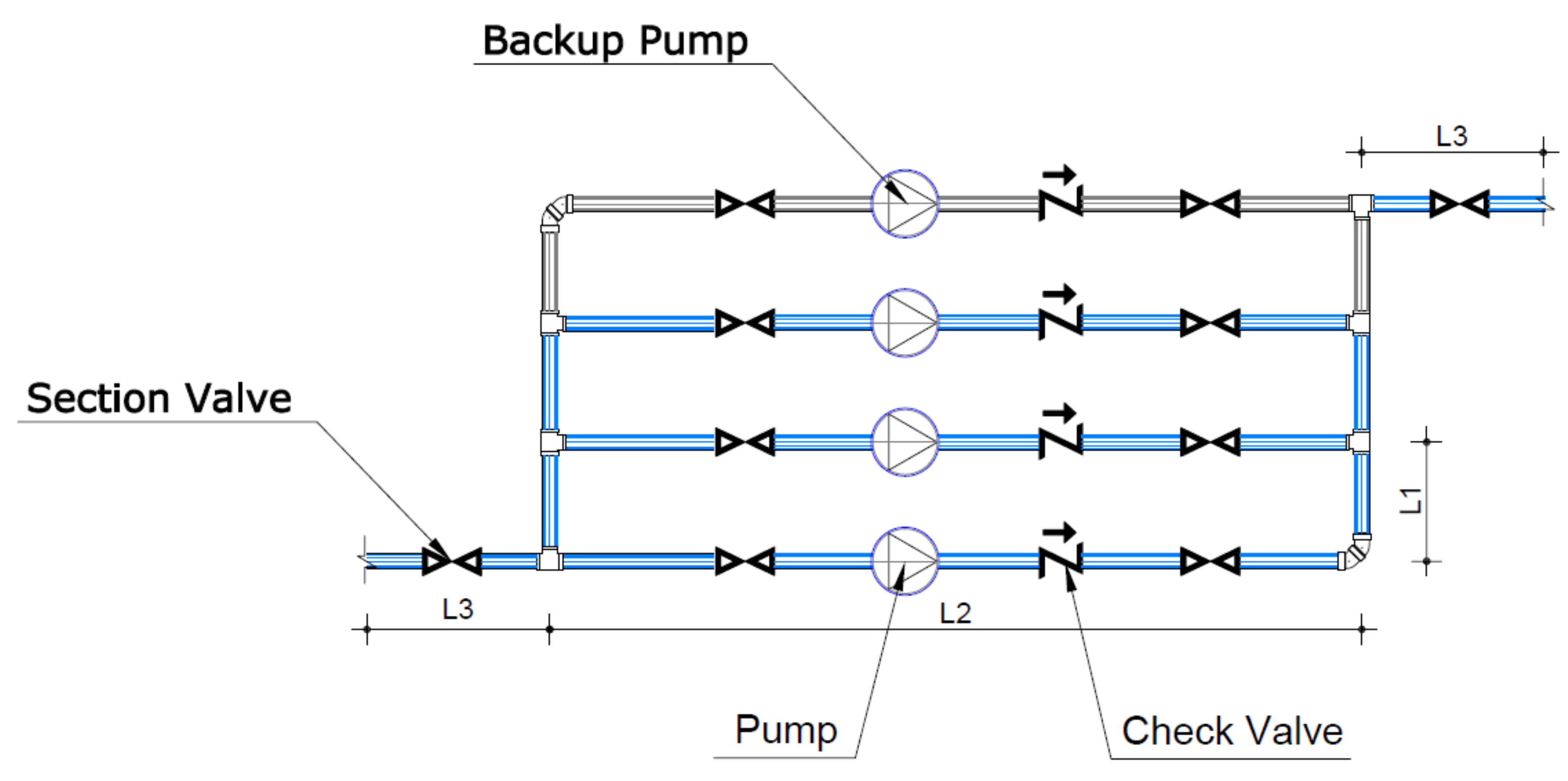
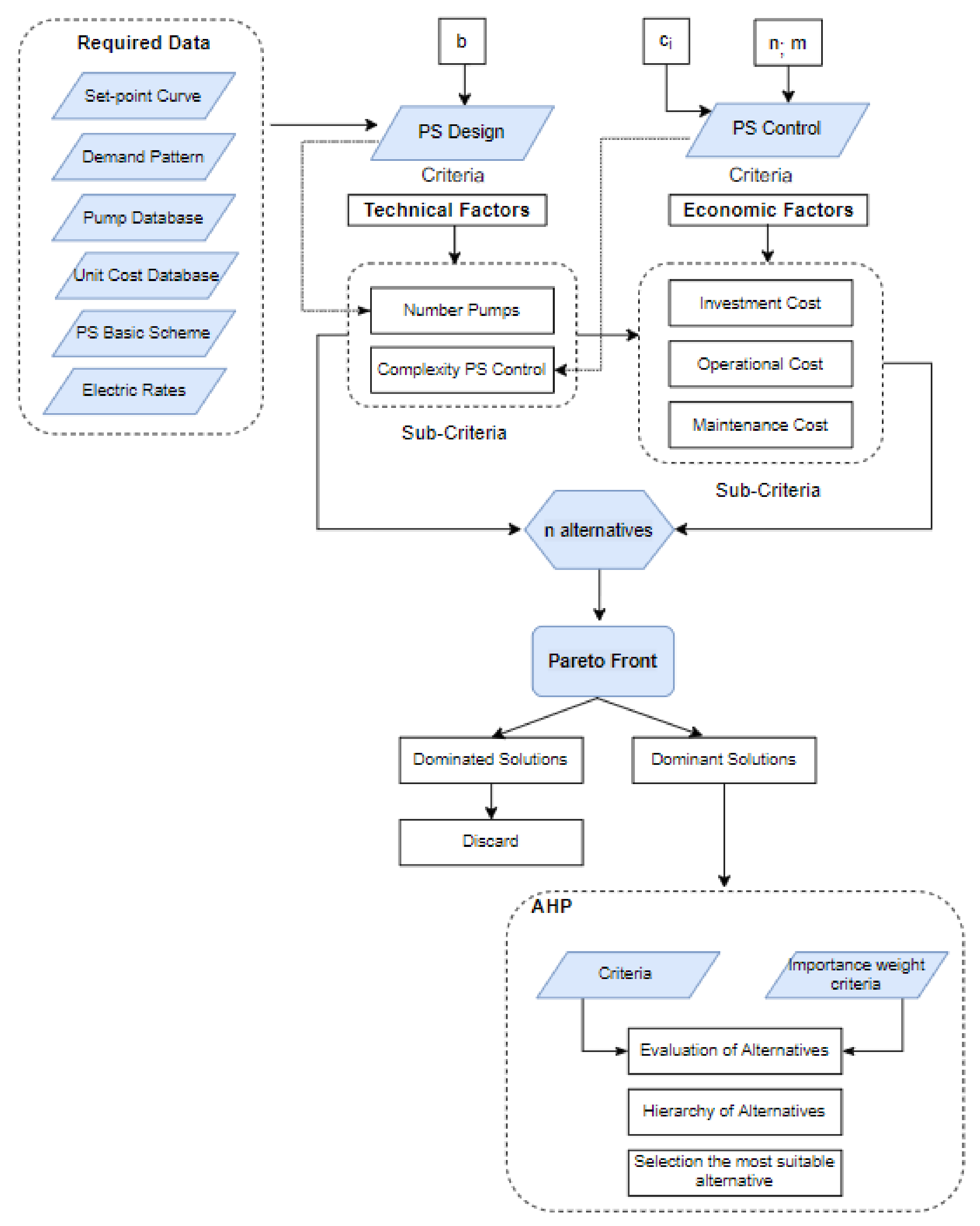
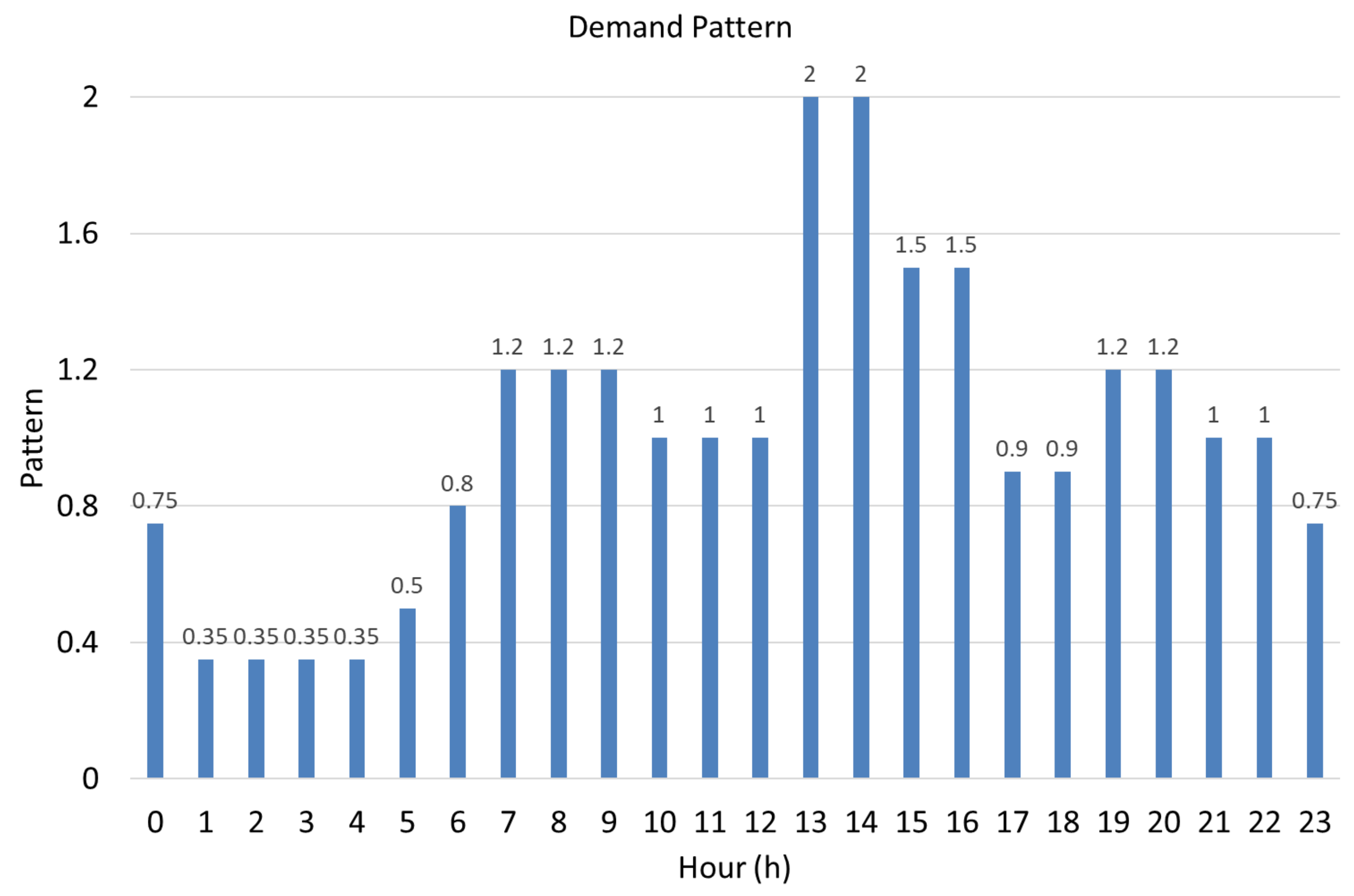
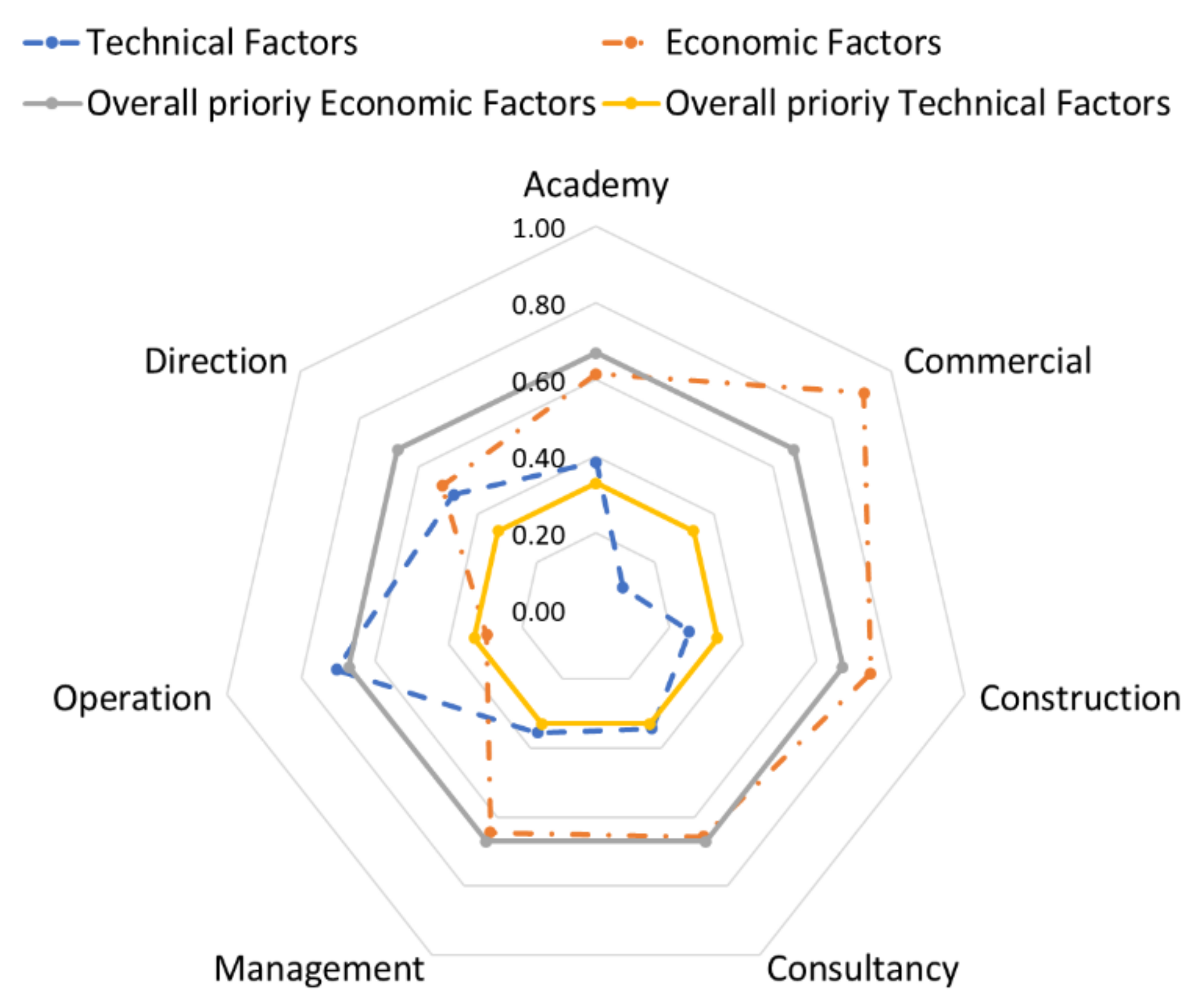
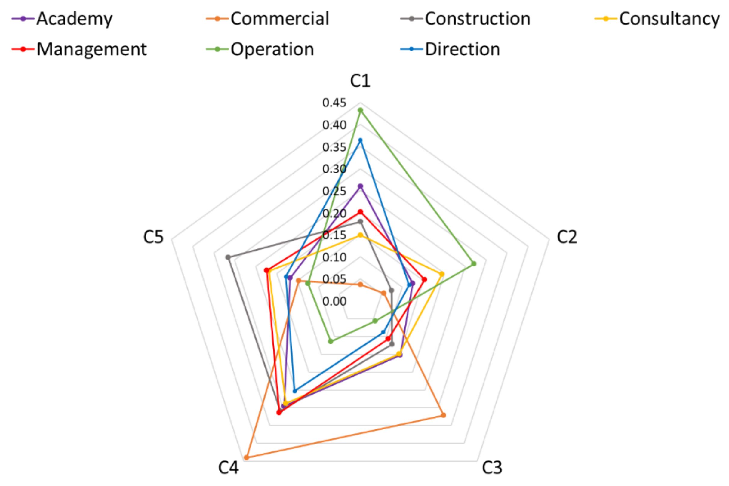
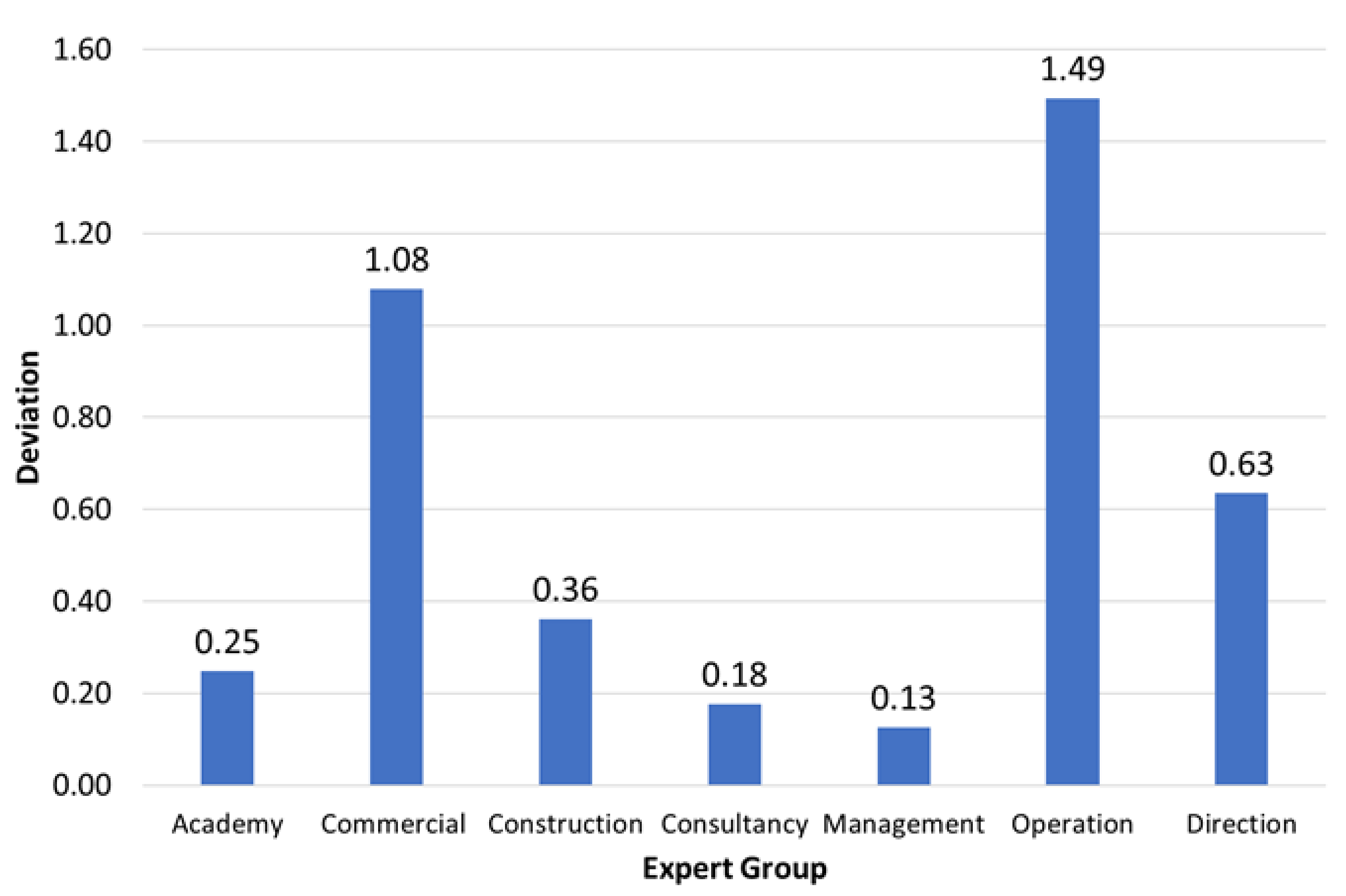
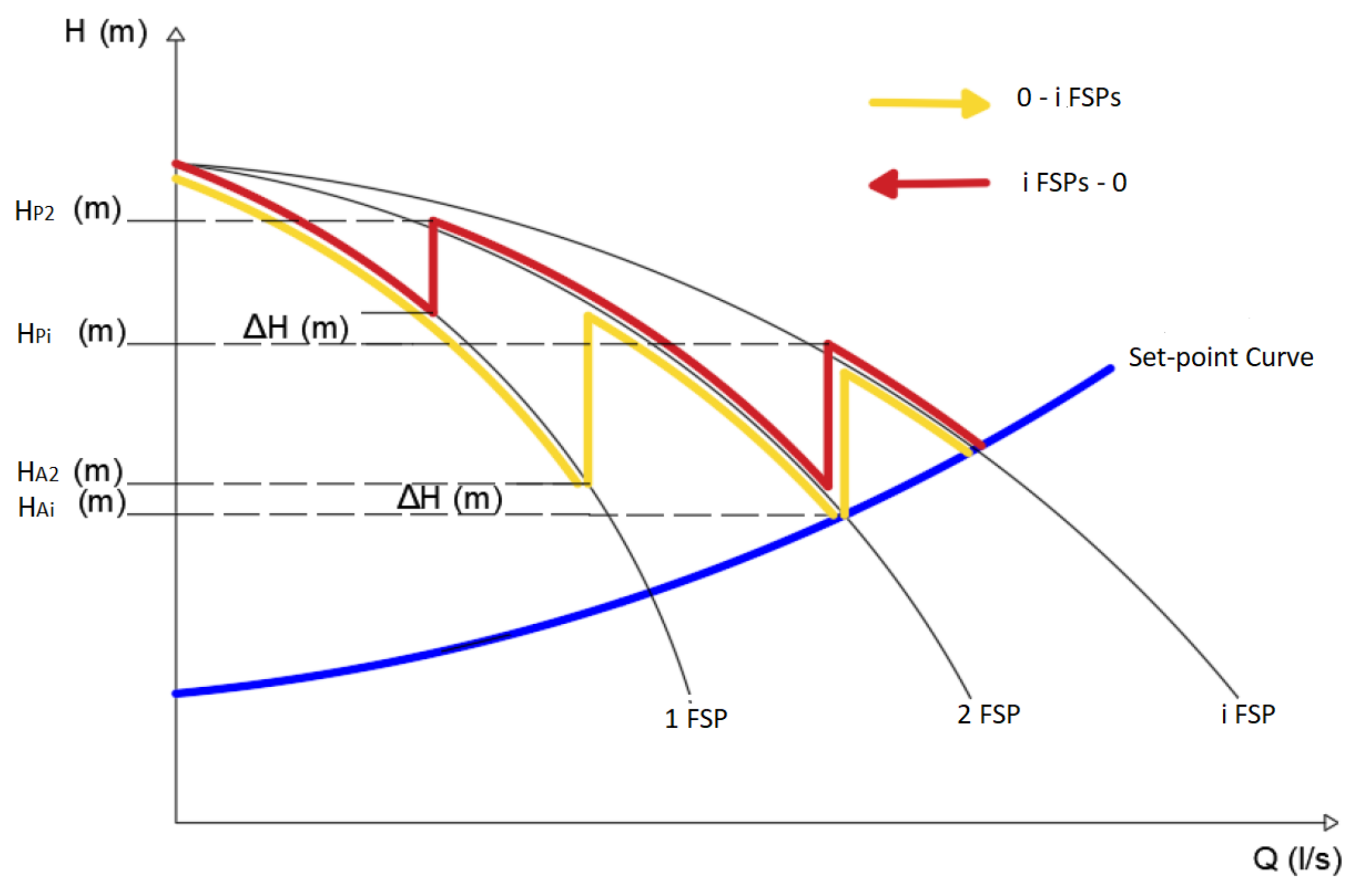
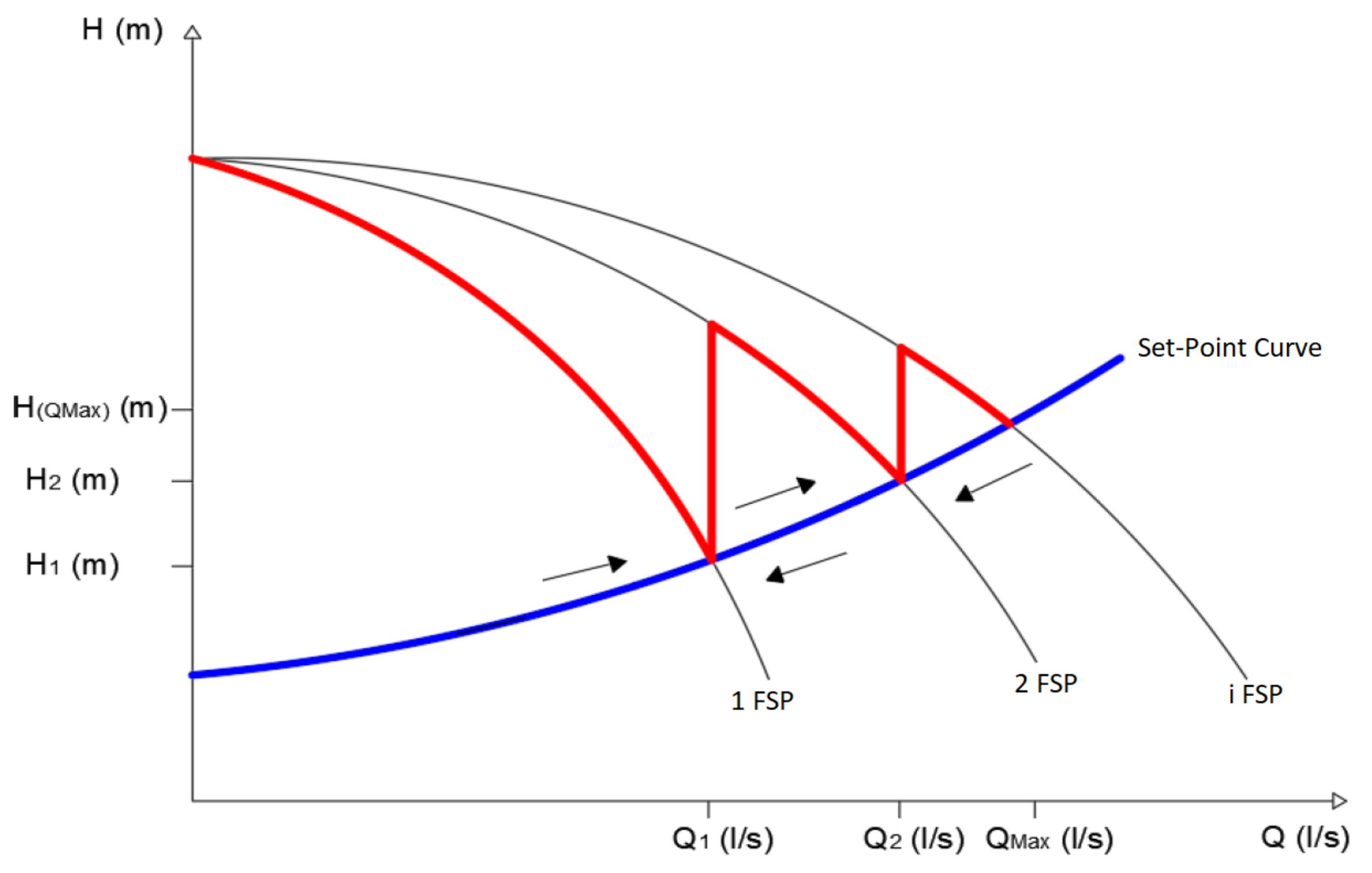
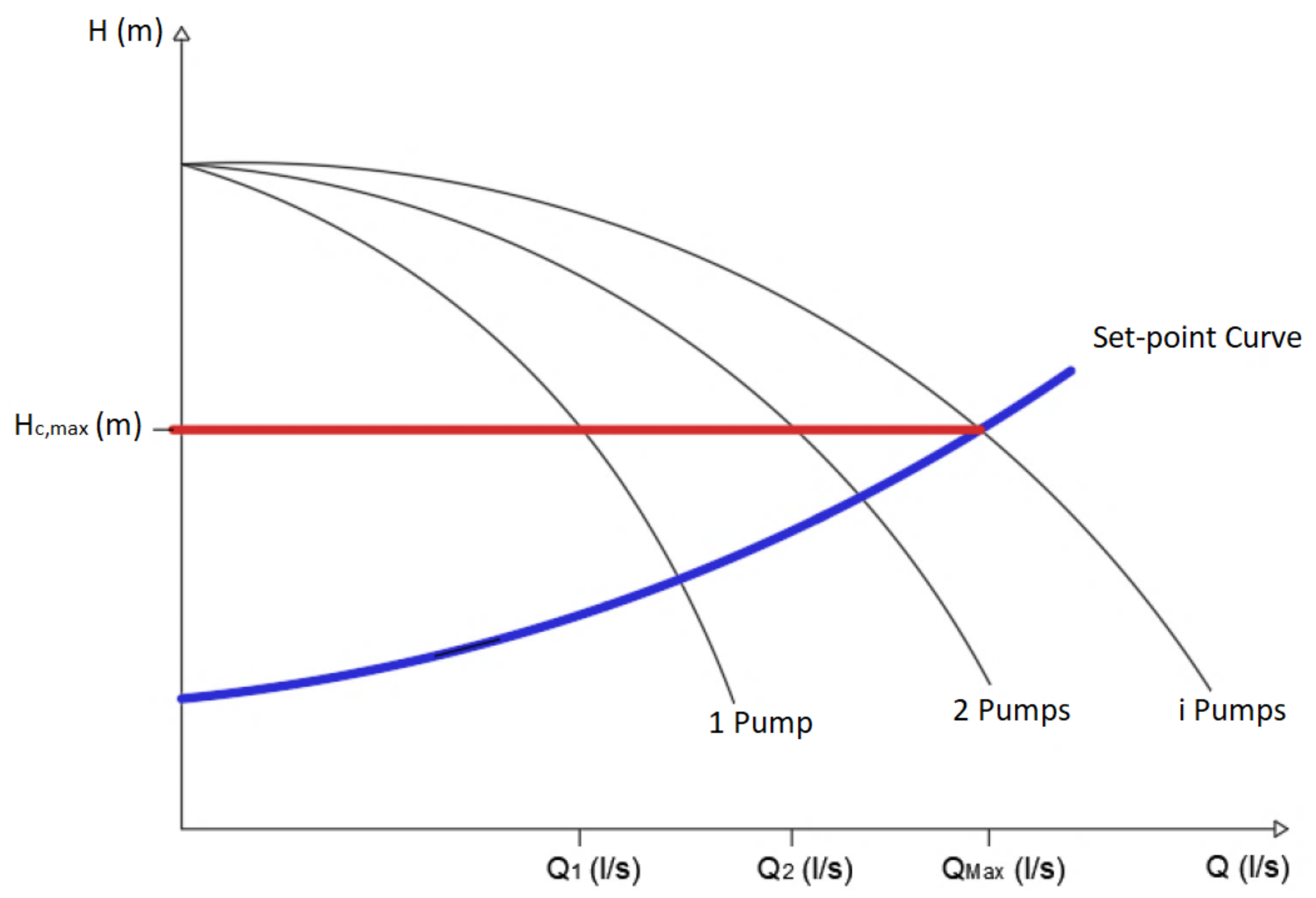
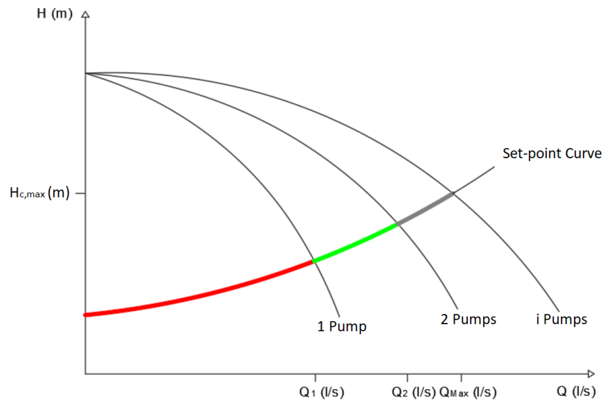
Table A1.
Function cost of different elements in a PS.
| Element | C(X) (EUR) | X | C1 | C2 | C3 |
|---|---|---|---|---|---|
| Pipe | ND (mm) | 10.13 | 0.20 | 0.0005 | |
| Elbow connector | ND (mm) | 29.17 | 0.01 | - | |
| Tee connector | ND (mm) | 42.60 | 0.01 | - | |
| Section Valve | ND (mm) | 63.63 | 0.79 | 0.01 | |
| Check Valve | ND (mm) | 35.63 | −0.14 | 0.01 | |
| Flow meter | Din (mm) | 885.70 | −9.22 | 0.06 | |
| Variable Frequency Drive | P (KW) | 168.19 | 116.08 | −0.60 |
The term C(X) is the function cost of the elements of the PS, x is the variable of every function cost. These variables could be: the nominal diameter (ND) or the internal diameter (Din) of these accessories, and the power (P) of the frequency drive. Finally, the terms C1, C2, and C3 are constant parameters of every function cost.
Maintenance Costs: These costs are related to the maintenance activities of the infrastructure of the PS, control system, and their frequency of implementation. This cost is expressed in annual form, so the frequency of implementation is defined as the number of times to implement the maintenance activities in a year.
The term CMaint is the annual maintenance cost of the PS. The term CUAPSi is the unit cost of the maintenance activities of the pump and the sub-term i is every maintenance activity of the pump. The terms fAPi and b are the annual frequency of maintenance and the number of pumps in the PS, respectively. The term CUpipe is the unit cost of the maintenance activity of the pipe. This cost is expressed in unit of length of the pipe (EUR/m). The terms fpipe and LT are the annual frequency of maintenance and the total length of the pipe, respectively. The term CUACCj is related to the unit cost of the maintenance activity of the accessories in the PS and the sub-term j is every one of these accessories (valves, elbow, and tee connectors). The terms fACCj and NACCj are the annual frequency of maintenance and the number of units of these accessories, respectively. Finally, is the unit cost of maintenance of every equipment of the control mode in the PS. The sub-term k is every one of the equipment of the control mode (pressure switch, flow meter, transducer pressure, PLC, and VFD). The terms fRMk and NRMk are the annual frequency of maintenance and the number of units of these devices of control, respectively. It is important to mention that every maintenance activity of the PS and their frequency of implementation is based on the recommendation for the factory of these elements. The unit cost is obtained from a database of maintenance costs.
Operational Cost: This cost is associated with the consumption energy by the PS in a year. This work considered two types of consumption energy in a year: Summer and Winter. Besides, every season has different energy tariffs concerning the type of hours, which are: peak off-hours, rush hours and plain hours. The following expression determines the operational cost.
The term COp is the operational cost of the PS in a year. The terms PT,i and PT,j corresponds to the consumed power of every hour in summer and winter, respectively. The terms hi and hj are the time interval in hours of summer and winter. CE,i and CE,j are the energy tariffs of every hour in summer and winter. The sub-terms i and j refer to every hour of a day in summer and winter and the term hT represents the 24 h of the day.
References
- Conti, J.; Holtberg, P.; Diefenderfer, J.; LaRose, A.; Turnure, J.T.; Westfall, L. International Energy Outlook 2016 with Projections to 2040. In International Energy Outlook 2016 with Projections; USDOE Energy Information Administration (EIA): Washington, DC, USA, 2016; Volume 0484. [Google Scholar]
- Tolvanen, H.J. Life cycle energy cost savings and pump selection. World Pumps 2007, 2007, 34–37. [Google Scholar] [CrossRef]
- Bunn, S. Pump Scheduling Optimization in Four US Cities: Case Studies. In Proceedings of the Eighth Annual Water Distribution Systems Analysis Symposium (WDSA), Cincinnati, OH, USA, 27–30 August 2006; pp. 1–12. [Google Scholar] [CrossRef]
- Cohen, D.; Shamir, U.; Sinai, G. Sensitivity analysis of optimal operation of irrigation supply systems with water quality considerations. Irrig. Drain. Syst. 2004, 18, 227–253. [Google Scholar] [CrossRef]
- McCormick, G.; Powell, R. Optimal Pump Scheduling in Water Supply Systems with Maximum Demand Charges. J. Water Resour. Plan. Manag. 2003, 129, 372–379. [Google Scholar] [CrossRef]
- Cimorelli, L.; D’Aniello, A.; Cozzolino, L. Boosting Genetic Algorithm Performance in Pump Scheduling Problems with a Novel Decision-Variable Representation. J. Water Resour. Plan. Manag. 2020, 146, 04020023. [Google Scholar] [CrossRef]
- Hashemi, S.S.; Tabesh, M.; Ataeekia, B. Ant-colony optimization of pumping schedule to minimize the energy cost using variable-speed pumps in water distribution networks. Urban Water J. 2013, 11, 335–347. [Google Scholar] [CrossRef]
- Abdallah, M.; Kapelan, Z. Iterative Extended Lexicographic Goal Programming Method for Fast and Optimal Pump Scheduling in Water Distribution Networks. J. Water Resour. Plan. Manag. 2017, 143, 04017066. [Google Scholar] [CrossRef]
- Abdallah, M.; Kapelan, Z. Fast Pump Scheduling Method for Optimum Energy Cost and Water Quality in Water Distribution Networks with Fixed and Variable Speed Pumps. J. Water Resour. Plan. Manag. 2019, 145, 04019055. [Google Scholar] [CrossRef] [Green Version]
- Luna, T.; Ribau, J.; Figueiredo, D.; Alves, R. Improving energy efficiency in water supply systems with pump scheduling optimization. J. Clean. Prod. 2019, 213, 342–356. [Google Scholar] [CrossRef]
- Carpitella, S.; Brentan, B.; Montalvo, I.; Izquierdo, J.; Certa, A. Multi-criteria analysis applied to multi-objective optimal pump scheduling in water systems. Water Supply 2019, 19, 2338–2346. [Google Scholar] [CrossRef] [Green Version]
- León-Celi, C.; Iglesias-Rey, P.L.; Martinez-Solano, F.J.; Mora-Melia, D. A Methodology for the Optimization of Flow Rate Injection to Looped Water Distribution Networks through Multiple Pumping Stations. Water 2016, 8, 575. [Google Scholar] [CrossRef] [Green Version]
- León-Celi, C.F.; Iglesias-Rey, P.L.; Martínez-Solano, F.J.; Savic, D. Operation of Multiple Pumped-Water Sources with No Storage. J. Water Resour. Plan. Manag. 2018, 144, 04018050. [Google Scholar] [CrossRef]
- Briceño-león, C.X.; Iglesias-Rey, P.L.; Martinez-Solano, F.J.; Mora-Melia, D. Use of Fixed and Variable Speed Pumps in Water Distribution Networks with Different Control Strategies. Water 2021, 479, 23. [Google Scholar]
- Mahar, P.S.; Singh, R.P. Optimal Design of Pumping Mains Considering Pump Characteristics. J. Pipeline Syst. Eng. Pr. 2014, 5, 04013010. [Google Scholar] [CrossRef]
- Bhave, P.R.; Gupta, R. Optimal design of water distribution networks for fuzzy demands. Civ. Eng. Environ. Syst. 2004, 21, 229–245. [Google Scholar] [CrossRef]
- Nault, J.; Papa, F. Lifecycle Assessment of a Water Distribution System Pump. J. Water Resour. Plan. Manag. 2015, 141, 1–9. [Google Scholar] [CrossRef]
- Walski, T.; Creaco, E. Selection of Pumping Configuration for Closed Water Distribution Systems. J. Water Resour. Plan. Manag. 2016, 142, 04016009. [Google Scholar] [CrossRef]
- Walski, T.M. Planning-Level Capital Cost Estimates for Pumping. J. Water Resour. Plan. Manag. 2012, 138, 307–310. [Google Scholar] [CrossRef]
- Diao, K.; Sitzenfrei, R.; Rauch, W. The Impacts of Spatially Variable Demand Patterns on Water Distribution System Design and Operation. Water 2019, 11, 567. [Google Scholar] [CrossRef] [Green Version]
- Martin-Candilejo, A.; Santillán, D.; Iglesias, A.; Garrote, L. Optimization of the Design of Water Distribution Systems for Variable Pumping Flow Rates. Water 2020, 12, 359. [Google Scholar] [CrossRef] [Green Version]
- Greco, S.; Figueira, J.; Ehrgott, M. Multiple Criteria Decision Analysis, 2nd ed.; Springer: New York, NY, USA, 2016. [Google Scholar]
- Saaty, T.L. The Analytic Hierarchy Process; McGraw-Hil: New York, NY, USA, 1980. [Google Scholar]
- Saaty, T.L. Decision making with the analytic hierarchy process. Int. J. Serv. Sci. 2008, 1, 83. [Google Scholar] [CrossRef] [Green Version]
- Ariff, H.; Salit, M.S.; Ismail, N.; Nukman, Y. Use of Analytical Hierarchy Process (AHP) for Selecting The Best Design Concept. J. Teknol. 2012, 49, 1–18. [Google Scholar] [CrossRef] [Green Version]
- Ahmed, M.; Qureshi, M.R.; Mallick, J.; Hasan, M.A.; Hussain, M. Decision Support Model for Design of High-Performance Concrete Mixtures Using Two-Phase AHP-TOPSIS Approach. Adv. Civ. Eng. 2019, 2019, 1–8. [Google Scholar] [CrossRef] [Green Version]
- Al-barqawi, H.; Zayed, T. Infrastructure Management: Integrated AHP/ANN Model to Evaluate Municipal Water Mains’ Performance. Infrastruct. Syst. 2008, 14, 305–318. [Google Scholar] [CrossRef]
- Aşchilean, I.; Badea, G.; Giurca, I.; Naghiu, G.S.; Iloaie, F.G. Choosing the Optimal Technology to Rehabilitate the Pipes in Water Distribution Systems Using the AHP Method. Energy Procedia 2017, 112, 19–26. [Google Scholar] [CrossRef]
- Karleuša, B.; Hajdinger, A.; Tadić, L. The Application of Multi-Criteria Analysis Methods for the Determination of Priorities in the Implementation of Irrigation Plans. Water 2019, 11, 501. [Google Scholar] [CrossRef] [Green Version]
- Saaty, T.L. Perspectives on the Theory and Practice of Decision Making with the Analytic Hierarchy Process. Sci. Iran 1994, 9, 215–229. [Google Scholar] [CrossRef]
- Ward, M.; Poleacovschi, C.; Perez, M. Using AHP and Spatial Analysis to Determine Water Surface Storage Suitability in Cambodia. Water 2021, 13, 367. [Google Scholar] [CrossRef]
- Khamudkhanov, M.; Abdullabekov, I.; Khamudkhanova, B.; Dusmatov, K.; Fayzullayev, K. Controls of the modes of operation of the pumping station with the application of frequency-controlled electric drive Controls of the modes of operation of the pumping station with the application of frequency-controlled electric drive. IOP Conf. Ser. Mater. Sci. Eng. 2020, 862, 062048. [Google Scholar] [CrossRef]
- Saaty, T.L. Rank from comparisons and from ratings in the analytic hierarchy/network processes. Eur. J. Oper. Res. 2006, 168, 557–570. [Google Scholar] [CrossRef]
- Iglesias-Rey, P.L.; Martínez-Solano, F.J.; Arango-Gil, F.; Lozano-Cortés, V. Methodology for the selection of pumping stations considering its mode of operation. In Proceedings of the 10th International Perspectives on Water Resources and the Environmental (IPWE), Cartagena, Colombia, 5–7 December 2018; Volume 13. [Google Scholar]
- Jensen Engineered Systems. Pump Station Design Guidelines, 2nd ed.; Jensen EngineeredSystems.com: Sparks, NV, USA, 2012; p. 34. [Google Scholar]
- Jayanthi, M.; Ravishankar, T. Techno economic evaluation of windmill for water pumping in coastal areas for aquaculture. Indian J. Fish 2005, 52, 413–419. [Google Scholar]
- Murugaperumal, K.; Vimal, P.A.D. Feasibility design and techno-economic analysis of hybrid renewable energy system for rural electrification. Sol. Energy 2019, 188, 1068–1083. [Google Scholar] [CrossRef]
- Vilotijević, V.; Karadžić, U.; Vujadinović, R.; Kovijanić, V.; Božić, I. An Improved Techno-Economic Approach to Determination of More Precise Installed Parameter for Small Hydropower Plants. Water 2021, 13, 2419. [Google Scholar] [CrossRef]
- Naval, N.; Yusta, J.M. Optimal short-term water-energy dispatch for pumping stations with grid-connected photovoltaic self-generation. J. Clean. Prod. 2021, 316, 128386. [Google Scholar] [CrossRef]
- Liu, X.; Li, N.; Mu, H.; Li, M.; Liu, X. Techno-energy-economic assessment of a high capacity offshore wind-pumped-storage hybrid power system for regional power system. J. Energy Storage 2021, 41, 102892. [Google Scholar] [CrossRef]
- Department of the Army Corps of Engineers United States. Structural and Architectural Design of Pumping Stations (Engineer Manual); Department of the Army Corps of Engineers United States: Washington, DC, USA, 1989.
- Leiby, V.M.; Burke, M.E. Energy Efficiency Best Practices for North American Drinking Water Utilities; Water Research Foundation: Albany, NY, USA, 2011. [Google Scholar]
- Celi, C.F.L. Optimization of Both Energy Use and Pumping Costs in Water Distribution Networks with Several Water Sources Using the Setpoint Curve. Ph.D. Thesis, Universitat Politécnica de Valencia, Valencia, Spain, 2018. [Google Scholar]
Figure 1.
The basic scheme of a PS.

Figure 2.
Flowchart of the proposed methodology.

Figure 3.
Demand Patter for TF-Network and CAT-Network.

Figure 4.
Importance weight of factors of every group of experts.

Figure 5.
Importance weight of criteria of every group of experts.

Figure 6.
Deviation values of every expert group.

Table 1.
Require equipment or device for different control systems.
| Control System | Frequency Inverter | Pressure Switches | Pressure Transducer | Flowmeter | PLC | No. Regulation Equipment | |
|---|---|---|---|---|---|---|---|
| 1.0 | Without regulation | 0 | |||||
| 2.1 | PC with FSPs | X | 1 | ||||
| 2.2 | FC with FSPs | X | X | 2 | |||
| 3.1 | PC with VSPs | X | X | X | 3 | ||
| 3.2 | FC with VSPs | X | X | X | X | 4 | |
| 4.1 | PC with FSPs and VSPs | X | X | X | 3 | ||
| 4.2 | FC with FSPs and VSPs | X | X | X | X | 4 | |
Table 2.
Regulation modes rating.
| Regulation Mode (i) | 1.0 | 2.1 | 2.2 | 3.1 | 3.2 | 4.1 | 4.2 | Complexity Assessment (Cci) | Rating (Ri) |
|---|---|---|---|---|---|---|---|---|---|
| 1.0 | 1 | 3 | 5 | 7 | 9 | 7 | 9 | 0.43 | 1.00 |
| 2.1 | 1/3 | 1 | 3 | 5 | 7 | 5 | 7 | 0.24 | 0.57 |
| 2.2 | 1/5 | 1/3 | 1 | 3 | 5 | 3 | 5 | 0.14 | 0.32 |
| 3.1 | 1/7 | 1/5 | 1/3 | 1 | 3 | 1 | 3 | 0.07 | 0.15 |
| 3.2 | 1/9 | 1/7 | 1/5 | 1/3 | 1 | 1/3 | 1 | 0.03 | 0.07 |
| 4.1 | 1/7 | 1/5 | 1/3 | 1 | 3 | 1 | 3 | 0.07 | 0.15 |
| 4.2 | 1/9 | 1/7 | 1/5 | 1/3 | 1 | 1/3 | 1 | 0.03 | 0.07 |
Table 3.
Electric tariff for different time zones.
| Time Zones | |||||
|---|---|---|---|---|---|
| Summer Season | Winter Season | ||||
| Type of Hours | Electric Tariff | From | To | From | To |
| Off-peak hours | 0.069 | 0 | 8 | 0 | 8 |
| Peak hours | 0.095 | 11 | 15 | 18 | 21 |
| Plain hours | 0.088 | 9 | 10 | 8 | 18 |
| 16 | 23 | 21 | 23 | ||
Table 4.
Demand flows for the different PSs.
| TF-PS1 | TF-PS2 | CAT-PS2 | CAT-PS3 | |
|---|---|---|---|---|
| Qm (l/s) | 35.00 | 24.44 | 18.00 | 37.00 |
| Qmin (l/s) | 12.30 | 8.60 | 6.30 | 13.00 |
| Qmax (l/s) | 70.00 | 48.88 | 36.00 | 74.00 |
Table 5.
Set-Point curve parameters for every PS.
| Data | TF-PS1 | TF-PS2 | CAT-PS2 | CAT-PS3 |
|---|---|---|---|---|
| ΔH | 25.00 | 28.00 | 25.00 | 22.00 |
| R | 0.0020 | 0.0059 | 0.0106 | 0.0015 |
Table 6.
Overall priority and priority of every criterion for every expert group.
| Overall | Academic | Commercial | Constructor | Consultancy | Management | Operation | Direction | ||
|---|---|---|---|---|---|---|---|---|---|
| TF | Technical Factor | 0.33 | 0.38 | 0.09 | 0.25 | 0.34 | 0.36 | 0.70 | 0.48 |
| EF | Economic Factor | 0.67 | 0.62 | 0.91 | 0.75 | 0.66 | 0.64 | 0.30 | 0.52 |
| C1 | Number of pumps | 0.20 | 0.26 | 0.04 | 0.18 | 0.15 | 0.20 | 0.43 | 0.36 |
| C2 | Control system complexity | 0.13 | 0.13 | 0.06 | 0.07 | 0.19 | 0.15 | 0.27 | 0.12 |
| C3 | Investment Cost | 0.14 | 0.15 | 0.32 | 0.12 | 0.15 | 0.11 | 0.06 | 0.09 |
| C4 | Operational Cost | 0.31 | 0.29 | 0.44 | 0.31 | 0.29 | 0.31 | 0.11 | 0.25 |
| C5 | Maintenance Cost | 0.21 | 0.17 | 0.15 | 0.32 | 0.22 | 0.22 | 0.12 | 0.18 |
Table 7.
Number of viable pumps and solutions numbers for every PS.
| Viable Solutions | Pareto Front | ||||
|---|---|---|---|---|---|
| No. Models | No. Solutions | No. Models | No. Final Solutions | Reduction Rate Solutions | |
| TF-PS1 | 43 | 471 | 12 | 49 | 89.60% |
| TF-PS2 | 39 | 359 | 14 | 40 | 88.86% |
| CAT-PS2 | 45 | 357 | 15 | 30 | 91.60% |
| CAT-PS3 | 45 | 490 | 7 | 31 | 93.67% |
Table 8.
Assessment of the criteria for each alternative (TF-PS1).
| Priory Weight of Factors | Technical Factors (0.33) | Economic Factors (0.67) | ||||||
|---|---|---|---|---|---|---|---|---|
| Priority Weight of Criteria | C1 (0.20) | C2 (0.13) | C3 (0.14) | C4 (0.31) | C5 (0.21) | |||
| Hierarchy | ID Model | No. Pumps bi | ni FSP | mi VSP | Complexity | Investment Cost (EUR) | Operational Cost (EUR/Year) | Maintenance Cost (EUR/Year) |
| 1 | B30 | 3 | 3 | 0 | 2.1 | EUR 77,091.61 | EUR 18,094.16 | EUR 1040.11 |
| 2 | B65 | 3 | 3 | 0 | 1.0 | EUR 100,767.32 | EUR 21,387.13 | EUR 1136.44 |
| 3 | B61 | 3 | 3 | 0 | 2.1 | EUR 109,645.45 | EUR 15,351.70 | EUR 1148.58 |
| 8 | B33 | 2 | 0 | 2 | 3.2 | EUR 76,896.63 | EUR 16,099.10 | EUR 1018.72 |
| 12 | B31 | 3 | 2 | 1 | 4.1 | EUR 81,049.03 | EUR 14,910.76 | EUR 1107.24 |
| 15 | B59 | 4 | 4 | 0 | 1.0 | EUR 120,430.57 | EUR 18,320.99 | EUR 1420.55 |
| 22 | B66 | 3 | 0 | 3 | 3.2 | EUR 126,266.96 | EUR 10,723.13 | EUR 1318.83 |
| 24 | B28 | 4 | 4 | 0 | 2.2 | EUR 98,748.70 | EUR 13,046.24 | EUR 1407.69 |
| 37 | B58 | 5 | 5 | 0 | 2.2 | EUR 145,699.82 | EUR 11,328.55 | EUR 1787.40 |
| 38 | B27 | 6 | 6 | 0 | 2.2 | EUR 134,865.79 | EUR 11,963.36 | EUR 1960.90 |
| 39 | B57 | 8 | 8 | 0 | 2.2 | EUR 205,690.01 | EUR 11,123.06 | EUR 2617.86 |
| 40 | B49 | 10 | 10 | 0 | 2.2 | EUR 243,678.07 | EUR 9936.37 | EUR 3178.36 |
Table 9.
Rating of the criteria and overall rating for each alternative (TF-PS1).
| Priory Weight of Factors | Technical Factors (0.33) | Economic Factors (0.67) | |||||
|---|---|---|---|---|---|---|---|
| Priority Weight of Criteria | C1 (0.20) | C2 (0.13) | C3 (0.14) | C4 (0.31) | C5 (0.21) | ||
| Hierarchy | ID Model | Rating N. Pumps | Rating Complexity | Rating Investment Cost | Rating Operational Cost | Rating Maintenance Cost | Final Rating |
| 1 | B30 | 0.88 | 0.57 | 0.95 | 0.71 | 0.93 | 1.00 |
| 2 | B65 | 0.88 | 1.00 | 0.83 | 0.60 | 0.89 | 1.00 |
| 3 | B61 | 0.88 | 0.57 | 0.79 | 0.80 | 0.89 | 1.00 |
| 8 | B33 | 1.00 | 0.07 | 0.95 | 0.78 | 0.94 | 0.98 |
| 12 | B31 | 0.88 | 0.15 | 0.93 | 0.82 | 0.90 | 0.96 |
| 15 | B59 | 0.75 | 1.00 | 0.74 | 0.70 | 0.78 | 0.96 |
| 22 | B66 | 0.88 | 0.07 | 0.71 | 0.95 | 0.82 | 0.94 |
| 24 | B28 | 0.75 | 0.32 | 0.84 | 0.88 | 0.79 | 0.94 |
| 37 | B58 | 0.63 | 0.32 | 0.61 | 0.93 | 0.64 | 0.85 |
| 38 | B27 | 0.50 | 0.32 | 0.66 | 0.91 | 0.57 | 0.80 |
| 39 | B57 | 0.25 | 0.32 | 0.31 | 0.94 | 0.31 | 0.62 |
| 40 | B49 | 0.00 | 0.32 | 0.12 | 0.98 | 0.10 | 0.48 |
Table 10.
Assessment of the criteria for each alternative (TF-PS2).
| Priory Weight of Factors | Technical Factors (0.33) | Economic Factors (0.67) | ||||||
|---|---|---|---|---|---|---|---|---|
| Priority Weight of Criteria | C1 (0.20) | C2 (0.13) | C3 (0.14) | C4 (0.31) | C5 (0.21) | |||
| Hierarchy | ID Model | No. Pumps bi | ni FSP | mi VSP | Complexity | Investment Cost (EUR) | Operational Cost (EUR/Year) | Maintenance Cost (EUR/Year) |
| 1 | B32 | 2 | 0 | 2 | 3.2 | EUR 40,033.75 | EUR 11,033.00 | EUR 890.95 |
| 4 | B29 | 3 | 3 | 0 | 2.1 | EUR 36,392.86 | EUR 14,103.42 | EUR 1022.96 |
| 9 | B60 | 3 | 3 | 0 | 2.1 | EUR 60,626.74 | EUR 11,562.38 | EUR 1131.43 |
| 10 | B30 | 3 | 0 | 3 | 3.2 | EUR 45,312.38 | EUR 9220.70 | EUR 1193.21 |
| 11 | B31 | 3 | 0 | 3 | 3.2 | EUR 47,703.25 | EUR 9194.79 | EUR 1193.21 |
| 23 | B63 | 3 | 2 | 1 | 4.1 | EUR 77,860.25 | EUR 10,228.48 | EUR 1198.55 |
| 24 | B61 | 3 | 0 | 3 | 3.1 | EUR 85,229.43 | EUR 9529.86 | EUR 1243.41 |
| 26 | B52 | 4 | 4 | 0 | 1.0 | EUR 66,574.52 | EUR 16,032.72 | EUR 1388.39 |
| 28 | B59 | 4 | 4 | 0 | 2.2 | EUR 68,867.09 | EUR 9965.95 | EUR 1483.99 |
| 32 | B62 | 4 | 2 | 2 | 4.1 | EUR 84,374.22 | EUR 9472.57 | EUR 1490.08 |
| 36 | B51 | 5 | 5 | 0 | 1.0 | EUR 76,708.45 | EUR 15,975.26 | EUR 1655.77 |
| 37 | B58 | 5 | 5 | 0 | 2.2 | EUR 79,132.91 | EUR 9269.51 | EUR 1751.38 |
| 39 | B28 | 6 | 6 | 0 | 2.2 | EUR 60,527.23 | EUR 11,276.87 | EUR 1918.87 |
| 40 | B50 | 7 | 7 | 0 | 2.2 | EUR 87,848.31 | EUR 9047.27 | EUR 2303.30 |
Table 11.
Rating of the criteria and overall rating for each alternative (TF-PS2).
| Priory Weight of Factors | Technical Factors (0.33) | Economic Factors (0.67) | |||||
|---|---|---|---|---|---|---|---|
| Priority Weight of Criteria | C1 (0.20) | C2 (0.13) | C3 (0.14) | C4 (0.31) | C5 (0.21) | ||
| Hierarchy | ID Model | Rating N. Pumps | Rating Complexity | Rating Investment Cost | Rating Operational Cost | Rating Maintenance Cost | Final Rating |
| 1 | B32 | 1.00 | 0.07 | 0.88 | 0.83 | 0.90 | 1.00 |
| 4 | B29 | 0.80 | 0.57 | 0.94 | 0.68 | 0.81 | 0.99 |
| 9 | B60 | 0.80 | 0.57 | 0.55 | 0.80 | 0.75 | 0.97 |
| 10 | B30 | 0.80 | 0.07 | 0.80 | 0.92 | 0.71 | 0.97 |
| 11 | B31 | 0.80 | 0.07 | 0.76 | 0.92 | 0.71 | 0.97 |
| 23 | B63 | 0.80 | 0.15 | 0.27 | 0.87 | 0.70 | 0.94 |
| 24 | B61 | 0.80 | 0.15 | 0.15 | 0.90 | 0.67 | 0.94 |
| 26 | B52 | 0.60 | 1.00 | 0.45 | 0.58 | 0.58 | 0.92 |
| 28 | B59 | 0.60 | 0.32 | 0.41 | 0.88 | 0.52 | 0.91 |
| 32 | B62 | 0.60 | 0.15 | 0.16 | 0.91 | 0.52 | 0.91 |
| 36 | B51 | 0.40 | 1.00 | 0.28 | 0.58 | 0.41 | 0.85 |
| 37 | B58 | 0.40 | 0.32 | 0.25 | 0.92 | 0.35 | 0.85 |
| 39 | B28 | 0.20 | 0.32 | 0.55 | 0.82 | 0.24 | 0.62 |
| 40 | B50 | 0.00 | 0.32 | 0.10 | 0.93 | 0.00 | 0.48 |
Table 12.
Assessment of the criteria for each alternative (CAT-PS2).
| Priory Weight of Factors | Technical Factors (0.33) | Economic Factors (0.67) | ||||||
|---|---|---|---|---|---|---|---|---|
| Priority Weight of Criteria | C1 (0.20) | C2 (0.13) | C3 (0.14) | C4 (0.31) | C5 (0.21) | |||
| Hierarchy | ID Model | No. Pumps bi | ni FSP | mi VSP | Complexity | Investment Cost (EUR) | Operational Cost (EUR/Year) | Maintenance Cost (EUR/Year) |
| 1 | B29 | 2 | 2 | 0 | 2.1 | EUR 26,857.50 | EUR 8709.77 | EUR 737.07 |
| 2 | B33 | 1 | 0 | 1 | 3.2 | EUR 36,172.84 | EUR 7584.03 | EUR 601.57 |
| 3 | B60 | 2 | 2 | 0 | 2.1 | EUR 45,032.91 | EUR 7529.47 | EUR 845.53 |
| 8 | B30 | 2 | 0 | 2 | 3.2 | EUR 33,929.54 | EUR 6267.96 | EUR 890.95 |
| 11 | B31 | 2 | 0 | 2 | 3.1 | EUR 34,140.13 | EUR 7678.38 | EUR 832.69 |
| 14 | B61 | 2 | 0 | 2 | 3.1 | EUR 62,754.16 | EUR 6476.45 | EUR 941.16 |
| 15 | B28 | 3 | 3 | 0 | 2.2 | EUR 35,755.30 | EUR 8198.96 | EUR 1097.85 |
| 16 | B58 | 3 | 3 | 0 | 1.0 | EUR 52,068.90 | EUR 10,959.26 | EUR 1110.71 |
| 21 | B59 | 3 | 0 | 3 | 3.2 | EUR 66,803.39 | EUR 5229.30 | EUR 1293.10 |
| 22 | B62 | 3 | 0 | 3 | 3.1 | EUR 73,330.86 | EUR 6405.97 | EUR 1234.83 |
| 23 | B15 | 5 | 5 | 0 | 2.2 | EUR 43,682.33 | EUR 8035.18 | EUR 1642.91 |
| 24 | B50 | 5 | 5 | 0 | 2.2 | EUR 66,086.69 | EUR 6721.67 | EUR 1751.38 |
| 25 | B41 | 5 | 5 | 0 | 2.2 | EUR 64,990.43 | EUR 7054.42 | EUR 1751.38 |
| 26 | B40 | 6 | 6 | 0 | 2.2 | EUR 68,421.27 | EUR 6627.74 | EUR 2027.34 |
| 27 | B38 | 8 | 8 | 0 | 2.2 | EUR 80,856.08 | EUR 5918.28 | EUR 2455.36 |
Table 13.
Rating of the criteria and overall rating for each alternative (CAT-PS2).
| Priory Weight of Factors | Technical Factors (0.33) | Economic Factors (0.67) | |||||
|---|---|---|---|---|---|---|---|
| Priority Weight of Criteria | C1 (0.20) | C2 (0.13) | C3 (0.14) | C4 (0.31) | C5 (0.21) | ||
| Hierarchy | ID Model | Rating N. Pumps | Rating Complexity | Rating Investment Cost | Rating Operational Cost | Rating Maintenance Cost | Final Rating |
| 1 | B29 | 0.86 | 0.57 | 1.00 | 0.76 | 0.88 | 1.00 |
| 2 | B33 | 1.00 | 0.07 | 0.86 | 0.84 | 0.94 | 1.00 |
| 3 | B60 | 0.86 | 0.57 | 0.73 | 0.84 | 0.83 | 1.00 |
| 8 | B30 | 0.86 | 0.07 | 0.90 | 0.93 | 0.81 | 0.98 |
| 11 | B31 | 0.86 | 0.15 | 0.89 | 0.83 | 0.84 | 0.97 |
| 14 | B61 | 0.86 | 0.15 | 0.48 | 0.92 | 0.79 | 0.96 |
| 15 | B28 | 0.71 | 0.32 | 0.87 | 0.80 | 0.72 | 0.96 |
| 16 | B58 | 0.71 | 1.00 | 0.63 | 0.61 | 0.72 | 0.96 |
| 21 | B59 | 0.71 | 0.07 | 0.42 | 1.00 | 0.64 | 0.94 |
| 22 | B62 | 0.71 | 0.15 | 0.32 | 0.92 | 0.66 | 0.94 |
| 23 | B15 | 0.43 | 0.32 | 0.75 | 0.81 | 0.49 | 0.94 |
| 24 | B50 | 0.43 | 0.32 | 0.43 | 0.90 | 0.44 | 0.94 |
| 25 | B41 | 0.43 | 0.32 | 0.45 | 0.88 | 0.44 | 0.93 |
| 26 | B40 | 0.29 | 0.32 | 0.40 | 0.91 | 0.32 | 0.92 |
| 27 | B38 | 0.00 | 0.32 | 0.22 | 0.95 | 0.13 | 0.92 |
Table 14.
Assessment of the criteria for each alternative (CAT-PS3).
| Priory Weight of Factors | Technical Factors (0.33) | Economic Factors (0.67) | ||||||
|---|---|---|---|---|---|---|---|---|
| Priority Weight of Criteria | C1 (0.20) | C2 (0.13) | C3 (0.14) | C4 (0.31) | C5 (0.21) | |||
| Hierarchy | ID Model | No. Pumps bi | ni FSP | mi VSP | Complexity | Investment Cost (EUR) | Operational Cost (EUR/Year) | Maintenance Cost (EUR/Year) |
| 1 | B28 | 3 | 3 | 0 | 1.0 | EUR 76,003.47 | EUR 18,694.99 | EUR 1036.55 |
| 7 | B33 | 2 | 0 | 2 | 3.1 | EUR 78,954.39 | EUR 18,257.10 | EUR 973.32 |
| 10 | B27 | 4 | 4 | 0 | 1.0 | EUR 92,400.92 | EUR 18,663.93 | EUR 1312.08 |
| 12 | B61 | 3 | 0 | 3 | 3.1 | EUR 125,959.65 | EUR 11,041.80 | EUR 1269.14 |
| 14 | B59 | 4 | 4 | 0 | 1.0 | EUR 120,430.57 | EUR 18,564.49 | EUR 1420.55 |
| 20 | B58 | 5 | 5 | 0 | 2.2 | EUR 145,699.82 | EUR 11,276.69 | EUR 1787.40 |
| 24 | B49 | 7 | 7 | 0 | 1.0 | EUR 173,427.47 | EUR 16,154.81 | EUR 2255.73 |
Table 15.
Rating of the criteria and overall rating for each alternative (CAT-PS3).
| Priory Weight of Factors | Technical Factors (0.33) | Economic Factors (0.67) | |||||
|---|---|---|---|---|---|---|---|
| Priority Weight of Criteria | C1 (0.20) | C2 (0.13) | C3 (0.14) | C4 (0.31) | C5 (0.21) | ||
| Hierarchy | ID Model | Rating N. Pumps | Rating Complexity | Rating Investment Cost | Rating Operational Cost | Rating Maintenance Cost | Final Rating |
| 1 | B28 | 0.80 | 1.00 | 0.97 | 0.68 | 0.90 | 1.00 |
| 7 | B33 | 1.00 | 0.15 | 0.94 | 0.69 | 0.94 | 0.98 |
| 10 | B27 | 0.60 | 1.00 | 0.83 | 0.68 | 0.73 | 0.97 |
| 12 | B61 | 0.80 | 0.15 | 0.56 | 0.92 | 0.76 | 0.96 |
| 14 | B59 | 0.60 | 1.00 | 0.60 | 0.68 | 0.67 | 0.96 |
| 20 | B58 | 0.40 | 0.32 | 0.39 | 0.91 | 0.45 | 0.94 |
| 24 | B49 | 0.00 | 1.00 | 0.17 | 0.76 | 0.16 | 0.94 |
Table 16.
Obtained results in (TF-PS1) in the first alternative of conventional design (analyzing life cycle costs).
Table 16.
Obtained results in (TF-PS1) in the first alternative of conventional design (analyzing life cycle costs).
| Hierarchy | ID Model | bi N° Pumps | ni FSP | mi VSP | Control Mode | Investment Cost (EUR/Year) | Operational Cost (EUR/Year) | Maintenance Cost (EUR/Year) | Total Cost (EUR/Year) |
|---|---|---|---|---|---|---|---|---|---|
| 1 | B28 | 4 | 2 | 2 | 4.2 | EUR 7021.77 | EUR 10,259.15 | EUR 1472.04 | EUR 18,754.75 |
Table 17.
Obtained results in (TF-PS1) in the second alternative of conventional design (fixing the number of pumps).
Table 17.
Obtained results in (TF-PS1) in the second alternative of conventional design (fixing the number of pumps).
| Design Method | ID Model | bi | ni FSP | mi VSP | Control Mode | Investment Cost (EUR/Year) | Operational Cost (EUR/Year) | Maintenance Cost (EUR/Year) | Cycle Life Cost (EUR/Year) |
|---|---|---|---|---|---|---|---|---|---|
| Cycle Life Cost | B27 | 6 | 2 | 4 | 4.2 | EUR 8741.36 | EUR 10,707.82 | EUR 2025.25 | EUR 21,474.43 |
Publisher’s Note: MDPI stays neutral with regard to jurisdictional claims in published maps and institutional affiliations. |
© 2021 by the authors. Licensee MDPI, Basel, Switzerland. This article is an open access article distributed under the terms and conditions of the Creative Commons Attribution (CC BY) license (https://creativecommons.org/licenses/by/4.0/).
Share and Cite
MDPI and ACS Style
Briceño-León, C.X.; Sanchez-Ferrer, D.S.; Iglesias-Rey, P.L.; Martinez-Solano, F.J.; Mora-Melia, D. Methodology for Pumping Station Design Based on Analytic Hierarchy Process (AHP). Water 2021, 13, 2886. https://doi.org/10.3390/w13202886
AMA Style
Briceño-León CX, Sanchez-Ferrer DS, Iglesias-Rey PL, Martinez-Solano FJ, Mora-Melia D. Methodology for Pumping Station Design Based on Analytic Hierarchy Process (AHP). Water. 2021; 13(20):2886. https://doi.org/10.3390/w13202886
Chicago/Turabian StyleBriceño-León, Christian X., Diana S. Sanchez-Ferrer, Pedro L. Iglesias-Rey, F. Javier Martinez-Solano, and Daniel Mora-Melia. 2021. "Methodology for Pumping Station Design Based on Analytic Hierarchy Process (AHP)" Water 13, no. 20: 2886. https://doi.org/10.3390/w13202886
Note that from the first issue of 2016, this journal uses article numbers instead of page numbers. See further details here.