
Modelling and Incorporating the Variable Demand Patterns to the Calibration of Water Distribution System Hydraulic Model


1
Scarce Resources and Circular Economy (ScaRCE), UniSA STEM, University of South Australia, Mawson Lakes, SA 5095, Australia
2
Future Industries Institute, University of South Australia, Mawson Lakes, SA 5095, Australia
3
South Australian Water Corporation, Adelaide, SA 5000, Australia
*
Author to whom correspondence should be addressed.
Water 2021, 13(20), 2890; https://doi.org/10.3390/w13202890
Submission received: 9 September 2021
/
Revised: 6 October 2021
/
Accepted: 12 October 2021
/
Published: 15 October 2021
(This article belongs to the Section Hydraulics and Hydrodynamics)
Abstract
:Calibration of a water distribution system (WDS) hydraulic model requires adjusting several parameters including hourly or sub-hourly demand multipliers, pipe roughness and settings of various hydraulic components. The water usage patterns or demand patterns in a 24-h cycle varies with the customer types and can be related to many factors including spatial and temporal factors. The demand patterns can also vary on a daily basis. For an extended period of hydraulic simulation, the modelling tools allows modelling of the variable demand patterns using daily multiplication factors. In this study, a linear modelling approach was used to handle the variable demand patterns. The parameters of the linear model allow modelling of the variable demand patterns with respect to the baseline values, and they were optimised to maximise the association with the observed data. This procedure was applied to calibrate the hydraulic model developed in EPANET of a large drinking water distribution system in regional South Australia. Local and global optimisation techniques were used to find the optimal values of the linear modelling parameters. The result suggests that the approach has the potential to model the variable demand patterns in a WDS hydraulic model and it improves the objective function of calibration.
1. Introduction
Drinking water utilities are aimed at continuously delivering good quality water with sufficient pressure to its customers at minimal cost [1]. Raw water after it has gone through several treatment processes is supplied to consumers via a water distribution system (WDS). A WDS is made up of various components such as pumps, valves, pipes, storage tanks, reservoirs and several fittings. The optimal configuration settings of these components are required to ensure maximum performance at minimal cost. Hydraulic models are frequently used to study and analyse the behaviour of a WDS. The applications of these models include, but are not limited to, the investigation of various management scenarios, extension of the WDS, determination of the optimal network settings and identification of the critical areas for rehabilitation [2]. Hence, a hydraulic model of a WDS acts as a decision support tool to improve the system’s performance and reliability. The reliability of hydraulic model predictions greatly depends on the level of calibration. Under different modelling applications, a different level of calibration is required; hence, it should be done based on the intended purpose of use of the model. Ormsbee and Lingireddy [3] suggested that a maximum deviation of 10% between the observed and the model-simulated values can be considered as a satisfactory calibration in most planning applications, while a deviation of 5% is highly desirable for system design, operation and the application of water quality modelling.
WDS hydraulic model calibration is performed by adjusting several parameters that control the hydraulic behaviour of the network. These parameters are adjusted such that the model closely represents the behaviour of the real system [4]. A well calibrated hydraulic model will reliably reproduce both flow and pressure values at the point of interest [5]. Hydraulic model calibration is a considerably complex task as there are a large number of parameters involved in the calibration process. Hence, manual calibration of a WDS hydraulic model can be a time-consuming task. The calibration of a WDS hydraulic model can be automated by incorporating readily available optimisation algorithms to the hydraulic model. These algorithms are broadly classified into local and global optimisation. A local optimisation searches the minimum value of the objective function within a local region of the input space. In contrast, global optimisation searches the minimum objective function within the whole input space. A majority of the global optimisation algorithms, including the covariance matrix adaptation evolution strategy (CMAES) and the shuffled complex evolution (SCE), belong to the class of evolutionary algorithm, which is a population-based metaheuristic algorithm [6,7,8,9,10,11]. The gradient-based methods such as the Gauss–Levenberg–Marquardt algorithm (GLMA) are commonly used in local optimisation [12]. The global optimisation algorithms are proven to be very reliable, despite the limitation that they cannot effectively handle a large number of parameters [12].
There have been many studies that describe the detailed calibration procedure of a WDS hydraulic model [2,3,5,13,14,15]. The objective function of a WDS hydraulic model calibration is non-linear and the optimisation problem can be considered as ill-posed due to the fact that the number of measurements is much smaller than the variables [14,15]. Using a genetic algorithm (GA), Do et al. [15] proposed an approach to deal with the ill-posed problem and suggested that averaging the result of multiple simulation can be considered as a good solution. Khedr, Tolson and Ziemann [13] compared a manual vs an automatic approach using multiple objective functions where the better performance was achieved under automatic calibration using the pareto archived dynamically dimensioned search (PA-DDS) algorithm. Similarly, Do et al. [16] and Letting et al. [17] used particle swarm optimisation to estimate the water demand in a WDS hydraulic model. Liong and Atiquzzaman [6] compared the performance of several optimisation algorithms including SCE, GA and simulated annealing (SA) and concluded that SCE has the potential to optimise the WDS hydraulic model. An issue with the hydraulic simulation is that zero flows can cause a computation failure while solving the non-linear equations of the model [18]. Currently, hydraulic models are equipped with a low flow adjustment function to prevent the situation of the solution becoming ill-conditioned or not converged.
A major challenge faced by the water utilities is to manage water losses in the network that occur via leakage. According to a survey by the International Water Services Association (IWSA), between approximately 8 and 24% of water losses are due to leakage in most developed countries, while in developing countries this could be vary between 25 and 45% [19]. Several reasons can trigger leakage in the network including aging infrastructure, corrosion in pipes, mechanical damage due to excessive loads, material defects, assembling errors and seasonal variation in temperature [20,21,22]. There are various leakage analysis methods and management strategies available in the literature [20,22,23]. Water leaks in a WDS can affect the quality and quantity of water [20,22]. They can increase the operating cost of the network as more energy is required to ensure the minimum operating pressure. Leakage is also an environmental, sustainability and health and safety issue [22]. Hydraulic modelling tools allow the simulation of leakage in the network using an emitter connected to a junction. An emitter allows modelling of the flow through a nozzle or orifice that discharges water to the atmosphere. The discharge by the emitter is expressed using a power function of the nodal pressure. For each leakage node, an emitter coefficient and a global emitter exponent are used to model the leakage flow, and they are optimised to represent the leakage more accurately. However, this study focused on modelling variable demand patterns and leakage was excluded from the analysis considering the current optimisation problem size. This is because several additional parameters need to be included in the model to simulate the leakage in the network and calibrating all of them with the other model parameters would be computationally very extensive.
Sustainability and efficiency are two major aspects that need to be considered while optimising a hydraulic model. The performance of a WDS can be assessed using several key performance indicators (KPIs) including the quality of and access to the services, efficiency in operation and business management, and financial and environmental sustainability [24,25,26]. A study by Dandy et al. [27] suggested that optimising a WDS with consideration of the KPI variables can significantly reduce the CO2 emissions and consumption of non-renewable resources. While a water column is moving through the pipe network, it involves energy expenditure and minimum energy is sought for sustainability and efficiency aspects. A WDS subjected to low flows with high frequency can potentially reduce the energy footprint and CO2 emissions [26]. Controlling the pressure throughout the network also helps to improve the efficiency of the system [26]. The calibration objective function of a WDS hydraulic model should constitute the KPI variables to ensure sustainability and efficiency. While developing a hydraulic model, the operating rules in the model should be defined to reflect the KPIs. For instance, pump operating rules should be aligned with the minimum energy price of the day in cases where the energy price changes throughout the day to ensure cost and energy efficiency. Similarly, tank operating rules should be defined such that they correspond to a minimum water age to ensure the quality of water. The parameters representing the variable demand patterns in a WDS hydraulic model can be used with other available KPIs to formulate the objective function and optimise the model parameters.
A WDS serves a variety of customers, hence, different consumption patterns are observed in different parts of the network. Typical consumption patterns in a WDS are classified as residential, commercial and industrial [17]. These patterns are comprised by multiplication factors that represent the hourly or sub-hourly water consumption within a 24-h cycle with respect to a baseline value. Among these patterns, the residential demand pattern is highly variable in space and time and probably one of the most dominating factors controlling the hydraulic behaviour of the network. According to Kang and Lansey [28], water demand and pipe roughness are the most uncertain parameters as they are not directly measurable. Therefore, successful calibration mostly depends on the fine tuning of these parameters. Data analysis shows that variable demand patterns for an extended period of hydraulic simulation can be better modelled using a linear modelling approach than using the multiplication factors only. Therefore, the objectives of the study are: (i) to develop a WDS hydraulic model and to incorporate variable demand patterns using linear modelling and (ii) to access the calibration performance under different optimisation algorithms. The proposed strategy has not been investigated before, hence, it brings a new knowledge to WDS hydraulic modelling.
2. Materials and Methods
2.1. Study Area
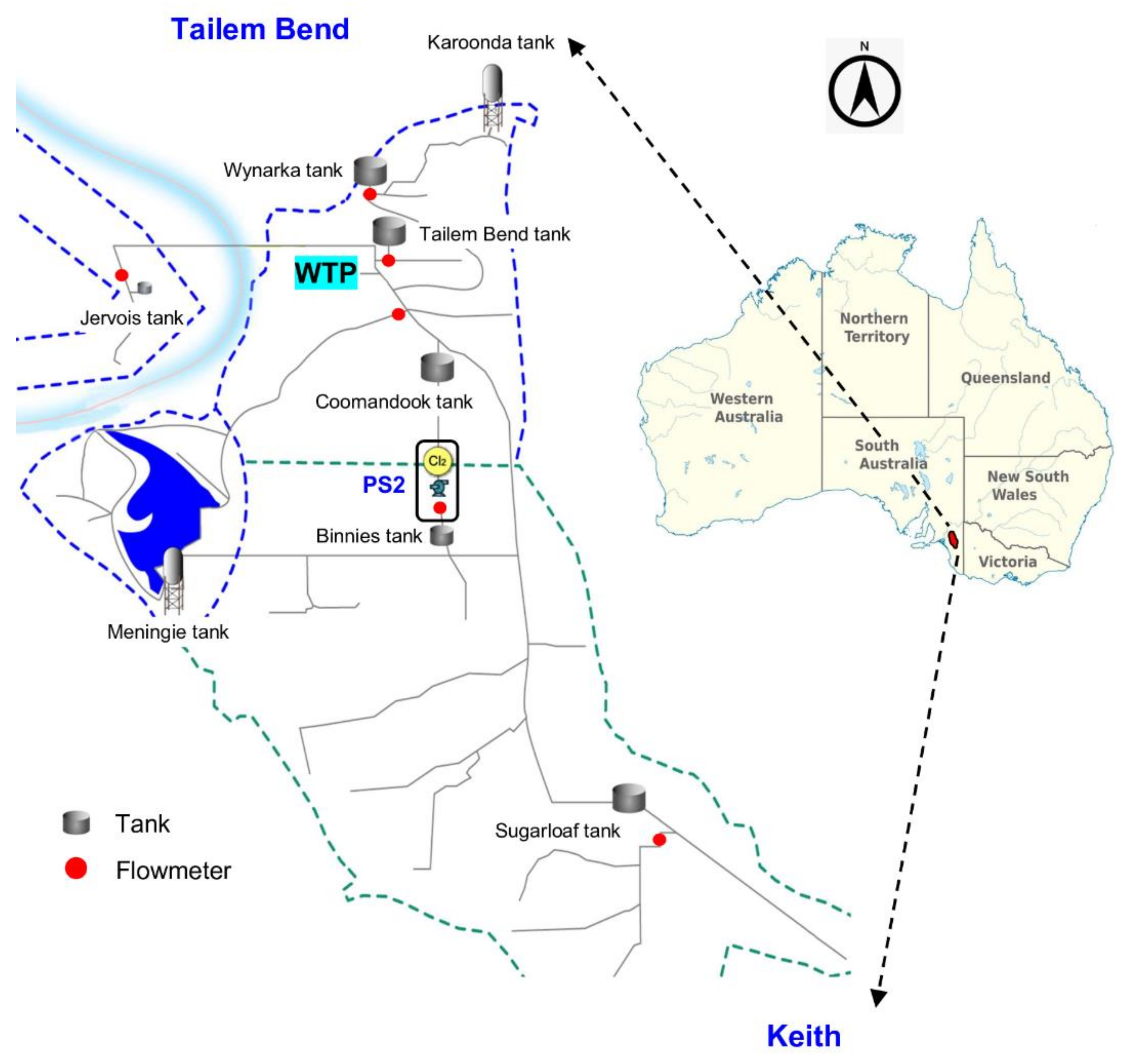
The study was conducted at Tailem Bend drinking water distribution system, which is one of the major drinking water distribution systems operated in regional South Australia (Figure 1). Water is withdrawn from River Murray, treated by a conventional treatment process, and then pumped into the distribution network consisting of about 143 km of pipeline and several hundred kilometres of branch mains [29]. Its supply network starts from Tailem Bend township and extends up to Keith with the treatment plant (WTP) located at the Tailem Bend township. On the way from Tailem Bend to Keith, the Tailem Bend–Keith (TBK) distribution system supplies drinking water in many intermediate locations including Lower Lakes, Binnies, Meningie and Sugarloaf Hill. The strategic locations of the distribution system are monitored by a supervisory control and data acquisition (SCADA) system that stores real-time monitoring data to the database server. It monitors a wide range of network configurations such as tank levels, pump status, valve status, pressure and flows. The location map and the schematic of the distribution system is presented in Figure 1.
2.2. Hydraulic Modelling Tool
EPANET, a WDS modelling tool developed by the U.S. Environmental Protection Agency (USEPA), was used to build the hydraulic model. Its hydraulic solver computes the nodal head and link flows by simultaneously solving the mass conservation equation for each node and the energy equation for each link in the network [30,31].
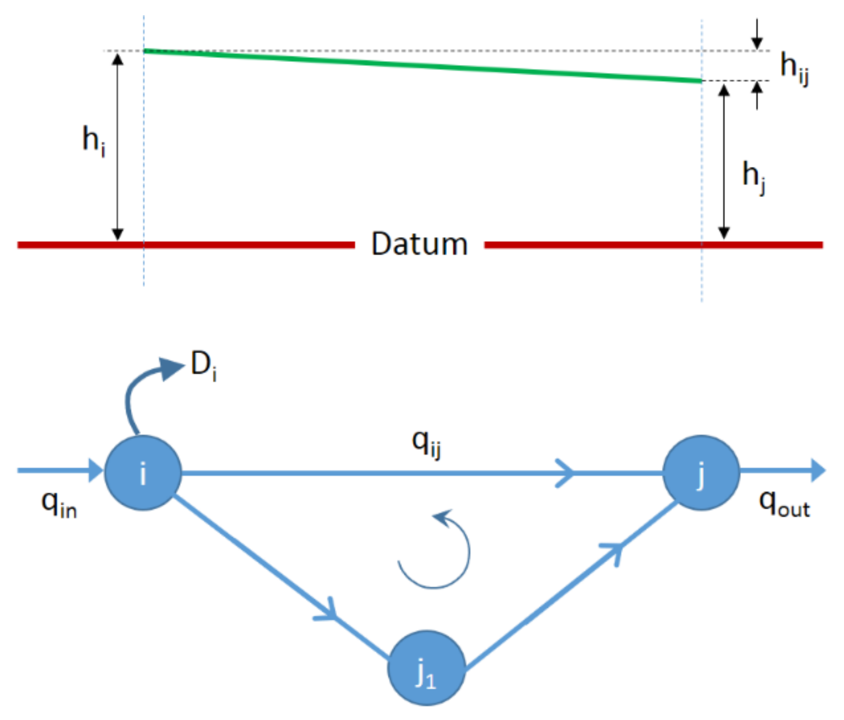
As shown in Figure 2, the conservation of mass requires that total inflow to a given node is equal to total outflow from that node, hence
where is the flow in pipe connecting nodes i and j and the summation is performed for all nodes, j connected to node i, is the demand or water consumed at node i.
The conservation of energy in a link between nodes i and j is given by
where represent head loss in pipe between the nodes, and are hydraulic heads at node i and j, r is a head loss coefficient whose value depends on the friction head-loss formula being used, n is a flow exponent and m is a minor loss coefficient. For a pump between node i and j, the head loss is calculated as
where is pump relative speed factor, is the pump usual head when not operating and , are pump curve coefficients.
The head loss coefficient, r, along the pipe is calculated by using one of the three methods: (i) Hazen–Williams formula (suitable to model flow under average conditions such as turbulent flow with temperature between 60 and 75° F and viscosity similar to water); (ii) Darcy–Weisbach formula (suitable to model pressurized flow under a wide range of hydraulic conditions); (iii) Chezy–Manning formula (generally used for open channel flow) [31]. The global gradient algorithm (GGA) introduced by Todini and Pilati [32] is employed to solve these linearized systems of equations through iterative process until the convergence criterion is met. Water demand is modelled by assigning a baseline demand at nodes, which are multiplied by an adjustment factor for each hour within a 24-h cycle. Pumps are modelled using a head-discharge curve, which shows the maximum head to which a given flow can be delivered. EPANET can perform two types of hydraulic simulations: (i) steady state simulation and (ii) extended period simulation [31]. The steady state simulation provides a snapshot of the distribution system for a given point in time, while the extended period simulation performs continuous simulation of the system and provides temporal variability of the system’s characteristics during the period. EPANET can also be used in various water quality analyses such as tracking the movement of a reactive or non-reactive chemical species in the network system over time, simulation of water age and the decay behaviour of chemical species. It is a public domain software and can be easily incorporated into many parameter optimisation tools. The available source code compiles and runs in the high performance computing (HPC) environment.
2.3. Optimisation Tool
The optimisation tools used are: (i) Parameter ESTimation (PEST) suite and (ii) R programming language. PEST is a model-independent parameter optimisation tool developed by Watermark Numerical Computing [12]. This software is frequently used in calibrating models of different domains including surface- and groundwater-based models [33,34]. Calibration setup in PEST requires creation of three files: (i) instruction file, (ii) template file and (iii) control file. The instruction file contains the information on how to read the desired portion of a simulation result from the model output file. The template file is similar to an EPANET input file except the parameters to calibrate are placed between a marker delimiter. During the optimisation process, template file is used to generate the model input file by populating the marked parameters in it with different values supplied by the optimisation algorithm. The control file contains calibration settings information, including the problem size, definition of control variables, initial parameter values, upper and lower boundary, observed data and variables’ corresponding weights. For parallel processing, a run management file is required that contains the path information of master and slave directory and the communication protocol between them. The optimisation algorithm takes control of the hydraulic model throughout the optimisation process. It performs hundreds to thousands of model runs until a termination criterion is reached and returns the optimised values. The calibration objective function is to minimise the difference between the observed and the simulated values, which is given by
where is the weight assigned to the ith measurement, and are the observed and the simulated values, respectively, and n is the total number of data points. The minimum value of is zero which means a perfect fit. However, it is very unlikely to achieve a zero and, hence, minimum value is sought.
The optimisation process involves many iterations where a number of criteria can be applied to terminate the process. The termination criteria used are: (i) convergence of adjustable parameters to their optimal values (parameter convergence); (ii) insignificant relative parameter change over the successive iterations (function convergence); (iii) insignificant objective function reduction over successive iterations; (iv) exceedance of the upper limit of the number of optimisation iterations [12]. During calibration, the optimisation iteration continues until one of the termination criteria is met and returns an optimum parameter set.
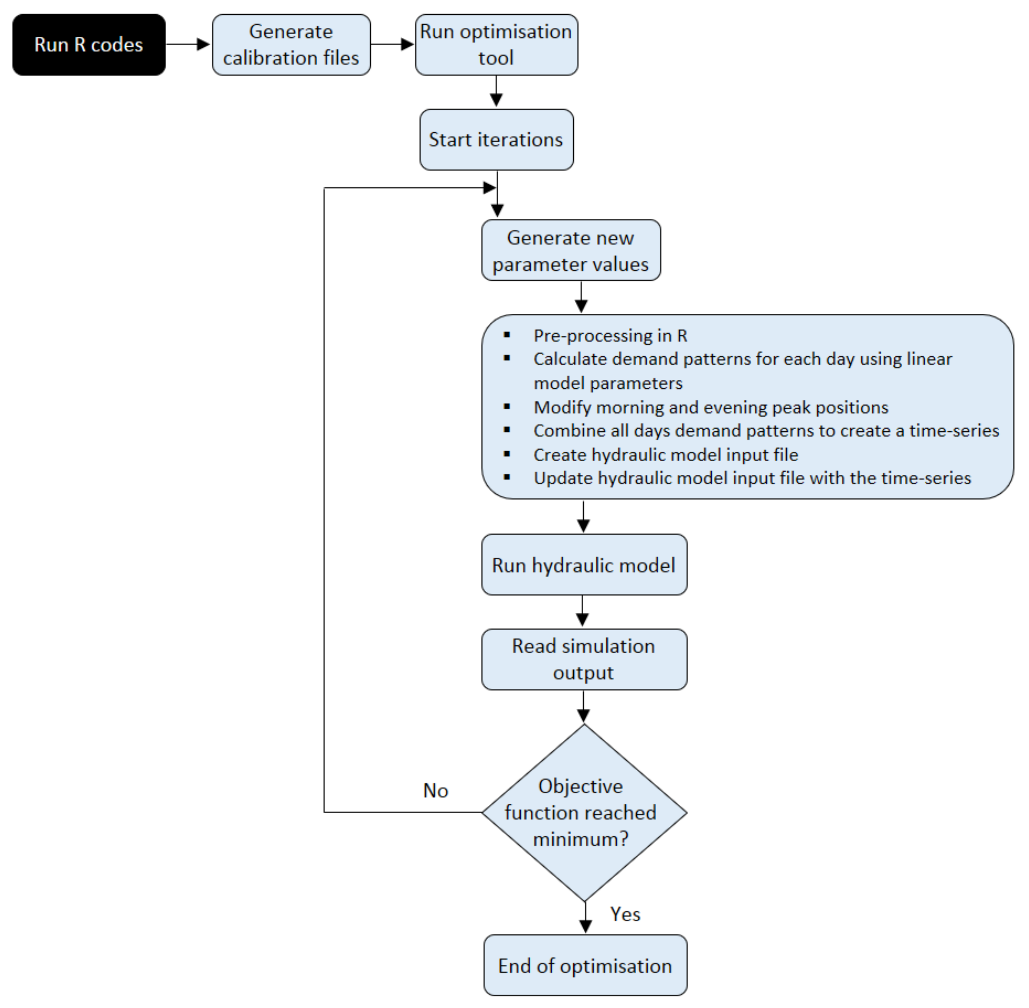
R is an open source programming language [35] used to perform various programming tasks with an extensive application in the field of statistical computing and graphics. Users can create specialized libraries and algorithms to manipulate data and/or to cope with the analysis requirements. In this study, R was used to create an interface between the optimisation tool and the hydraulic model and provide various settings’ information. Using this information, the necessary calibration files were generated for the desired period of simulation. During the optimisation iterations, the data sampled and returned by the optimisation algorithm were pre-processed in R prior to generating the hydraulic model input file. The interaction of these software and the flowchart of the procedure is shown in Figure 3.
2.4. Optimisation Algorithm
Both local and global optimisation were performed to find the minimum objective function. The GLMA algorithm built-in with PEST was employed in local search. In the algorithm, the parameter upgrade vector defines the direction and magnitude of the parameter adjustment in subsequent iterations. For a linear behaviour of the objective function, the parameter update vector is determined by gradient descent method where the direction of the vector is from the steepest descent of the objective function. For a non-linear behaviour of the objective function, Gauss–Newton method is applied where the upgrade vector is calculated based on the quadratic behaviour of the objective function. The linearity and non-linearity of the objective function is defined by a parameter called Marquardt lambda. A value of lambda greater than 10 indicates a linear behaviour of the objective function, while a value less than 2 indicates non-linear behaviour [12]. During the optimisation iterations, lambda is continuously updated to reduce the objective function to reach the local minima.
The global search methods used in the study were CMAES and SCE. The CMAES algorithm, proposed by Nikolaus Hansen, is generally used in optimising non-linear, non-convex, constrained or unconstrained problems in continuous domains [10]. This method is proven to be suitable in many different cases where derivative based methods, such as conjugate gradient or Quasi-Newton methods, fail due to a rugged search landscape (e.g., multi-modality, noisy, many local optima and outliers). The CMAES method is highly reliable in finding the local minima [10], while it is comparatively faster than many other evolutionary algorithms in finding the global minima [11].
CMAES minimizes the objective function through an iterative procedure where at each iteration, candidate solutions are generated according to a multivariate normal distribution. Three parameters are used to define the multivariate normal distribution, N(m, σ2, C) where m is the mean vector, σ is the step-size and C is the covariance matrix, which is a positive definite convex quadratic function, similar to the inverse Hessian matrix. The parameters m and σ determine the centre and spread of the distribution, while parameter C is mainly related to the shape of the distribution [36]. For each iteration, these candidate solutions and the corresponding objective functions are evaluated and ranked. Based on the rank, the parameters of the multivariate normal distribution are updated. The CMAES algorithm adaptively increases or decreases the search space in the next iteration based on the result of the previous iteration. The number of candidate solutions, referred to as population size, is the most critical strategy parameter. The default population size is given by 4 + 3 ln(n) where n is the number of variables to optimise. The population size needs to be increased in case of multi-modal and/or noisy objective function. The global search performance is improved by increasing the population size [37]. However, a large population size significantly increases the convergence time, while a relatively small population size allows faster convergence. The initial step-size, σ, should be carefully defined such that it can be reasonably applied to all variables.
SCE is a population-based stochastic optimisation algorithm introduced by Duan, Sorooshian and Gupta [9]. This method is based on four key concepts: (i) combination of deterministic and probabilistic approaches; (ii) grouping the sampled parameter sets into complexes and systematic evolution towards the direction of global improvement; (iii) competitive evolution; (iv) complex shuffling [8]. The optimisation process begins by generating several sets of random parameter values within their upper and lower boundary on the basis of a uniform probability distribution. Using each set of parameters, the model is run. and the objective function is evaluated. Based on the rank of the objective function value, these parameter sets are grouped into several complexes. A complex represents a local area of the whole domain where many individual local communities exist, similar to a genetic pool in GA [7]. Concurrent and independent searches are undertaken within these communities until each complex converges to its local minimum value. The feedback from each complex is collected into a common pool and re-ranks them by evaluating the objective function values. The parameter sets are then re-grouped and assigned to new complexes based on the new rank. The procedure is terminated once there is no significant improvement of the objective function value compared to the best objective function value found within a predefined number of iteration loops. The SCE algorithm maintains a balance between the search of the large solution space and the deep search of the sensitive locations [7].
In the same way as many global optimisation algorithms, random number generation drives much of the SCE optimisation process. Hence, choosing a different initial seed will lead to a different optimisation pathway [12]. Therefore, running the optimisation with a different initial seed can maximise the chance of finding the global minima. The SCE algorithm is more robust than traditional GA [38]. The sampling strategy involved in the SCE algorithm minimises the chance of being trapped in the local minima. However, it requires many more model runs to complete the optimisation process because the search does not always head straight downhill of the objective function terrain [12].
2.5. Hydraulic and Calibration Setup
The data required to set up the hydraulic model include initial states of various hydraulic components in the network and their geometry and settings information. The SCADA data from strategic locations of the network were used to configure the initial hydraulic states of the network. For calibration setup, observed time-series of flows and nodal heads at the points of interest were also required. All of these data were obtained from the South Australian Water Corporation (SA Water) who manage the TBK WDS network. The historic tank level data were expressed as a percentage full of the tank, which was subsequently converted to equivalent tank heads to make it compatible with EPANET. The SCADA data at the selected locations contained few missing values, which were estimated by linear interpolation method [39]. Additionally, data were checked for outliers and replaced them by the closest sensible values.
The Hazen–Williams formula was used to calculate pipe head loss. The hydraulic simulation time step and reporting time step in EPANET were set to 30 min, while the demand pattern time step was one hour. The necessary rules to simulate the behaviour of various hydraulic components in the model were defined. In the TBK WDS, historic time-series of some tank levels were found to have irregular empty and fill patterns. To accurately simulate the unsteady tank heads, several time-based control rules were defined, and they were also optimised. The model was divided into different zones and an overall correction factor was applied over the total nodal base demand for each zone.
Except for the built-in parameters in EPANET, some additional parameters were defined to adequately model the variable demand patterns. For each day of the simulation period, a linear modelling slope and intercept parameters were considered that relate the demand multipliers on that day with the baseline values, which could often be the average values from all days. However, by analysing the flow data during the study period, several demand patterns were identified, which were assigned to the model instead of assigning a global baseline value. Using the linear modelling parameters and the assigned patterns, the demand multipliers for all days were calculated. Additionally, to correct the position of morning and evening peaks on each day, two other parameters were utilised. The calculated demand multipliers of all days within the simulation period were then combined to create a time-series and the R codes were used to update the EPANET input file with the created time-series. The parameters that were optimised to calibrate the hydraulic model are presented in Table 1.
The initial values and the upper and lower boundary of the calibration parameters can considerably affect the number of model runs needed and the convergence time. An adequately defined initial value helps to reduce the number of iteration loops involved during the optimisation process. Majority of the initial values were acquired from the SCADA data, while the rest were decided from the modelling experience. The upper and lower boundaries of the demand multipliers and the linear modelling parameters were obtained by analysing the flowmeter readings during the simulation period. In deciding pipe roughness values, the age of the pipe was considered. The optimisation algorithms were run with different configuration settings (i.e., different population size, different number of complexes).
The PEST optimisation tool offers parameter transformation and suggests that using a combination of parameter transformation into natural and log domains can enhance the optimisation performance [12]. Therefore, in the calibration setup file, some parameters were randomly selected and defined to be log transformed, while others were in natural domain. Moreover, observation data such as flows and nodal head values have different numeric ranges that can make one variable become more sensitive than others, resulting in a different optimisation pathway being taken, led by the variable containing larger values. Hence, individual weight factor was assigned to each variable so that all observation variables had similar contribution to the objective function.
Model calibration requires hundreds to thousands of simulations with different parameter values in each simulation. Depending on the optimisation problem size, i.e., possible solution space by the number of parameters to calibrate, simulation period and the optimisation algorithm using, it can take several hours up to several days to complete the calibration process. To reduce the optimisation time, parallel processing was employed. The Linux-based tango 2.0 HPC (https://tango.unisa.edu.au/; accessed on January 2021) was used to perform the task. For this purpose, several software packages including EPANET and PEST were rebuilt to Linux compatible binaries from their source codes. In the Tango 2.0 system, computing task can be managed by using a bash script or using an interactive session. Programming codes were composed to create an interactive interface to view real-time information of calibration and the EPANET run status. GNU Linux screen utility was used to display the real-time output from the multiple parallel run windows in the same screen.
2.6. Goodness-of-Fit (GOF)
Standard GOF functions were used to evaluate the calibration performance. It is useful to assess the calibration performance using different GOF functions as the same optimisation can exhibit different levels of fit score under different GOF functions. There are several GOF functions available in the literature [34,40,41,42]. Among the various GOF functions, Nash–Sutcliffe efficiency (NSE) has been increasingly used in many areas including hydrological model evaluation, irrigation network system studies and optimising model parameters in different areas [34,41,42]. In this study, coefficient of determination (R2), root mean square error (RMSE) and NSE were used to assess the fit between the observed and the simulated time-series. These are given by the following equations
where and are the observed and simulated values for the flow and pressure, respectively, n is the total number of data points, and and are the means of the observed and simulated values, respectively. The value of NSE and R2 lies between 0 and 1, where 1 indicates perfect fit and 0 means no fit at all. On the other hand, a better calibrated model will encounter a relatively lower RMSE value.
3. Results and Discussion
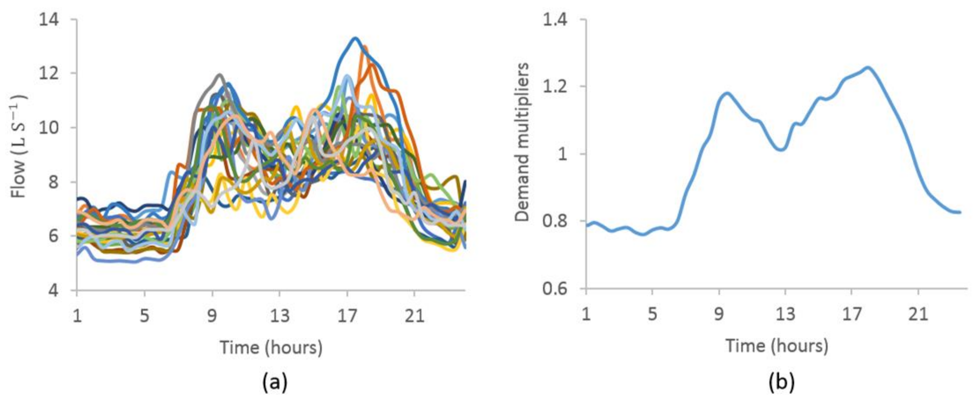
The EPANET hydraulic model for the TBK WDS was calibrated for a period of four weeks in early February–March, 2021. The flow pattern from a flowmeter during this period is presented in Figure 4a and the estimated average daily demand multipliers of all days are presented in Figure 4b. Both figures indicate the residential consumption mainly characterising the flow pattern in the area. There is a peak flow in the morning and in the evening, which is similar to a diurnal curve. A strong correlation was observed between the flows on different days with the correlation matrix ranged between 0.95 and 0.41. The maximum and minimum flows during this period were 13.29 L S−1 and 5.06 L S−1, respectively, with a mean value of 7.94 L S−1 and standard deviation of 1.64 L S−1. Several reasons, including seasonal variation of temperature, the day in the week (weekdays or weekend) and holidays can influence people’s water consumption pattern; hence, the demand multipliers on different days can also change.
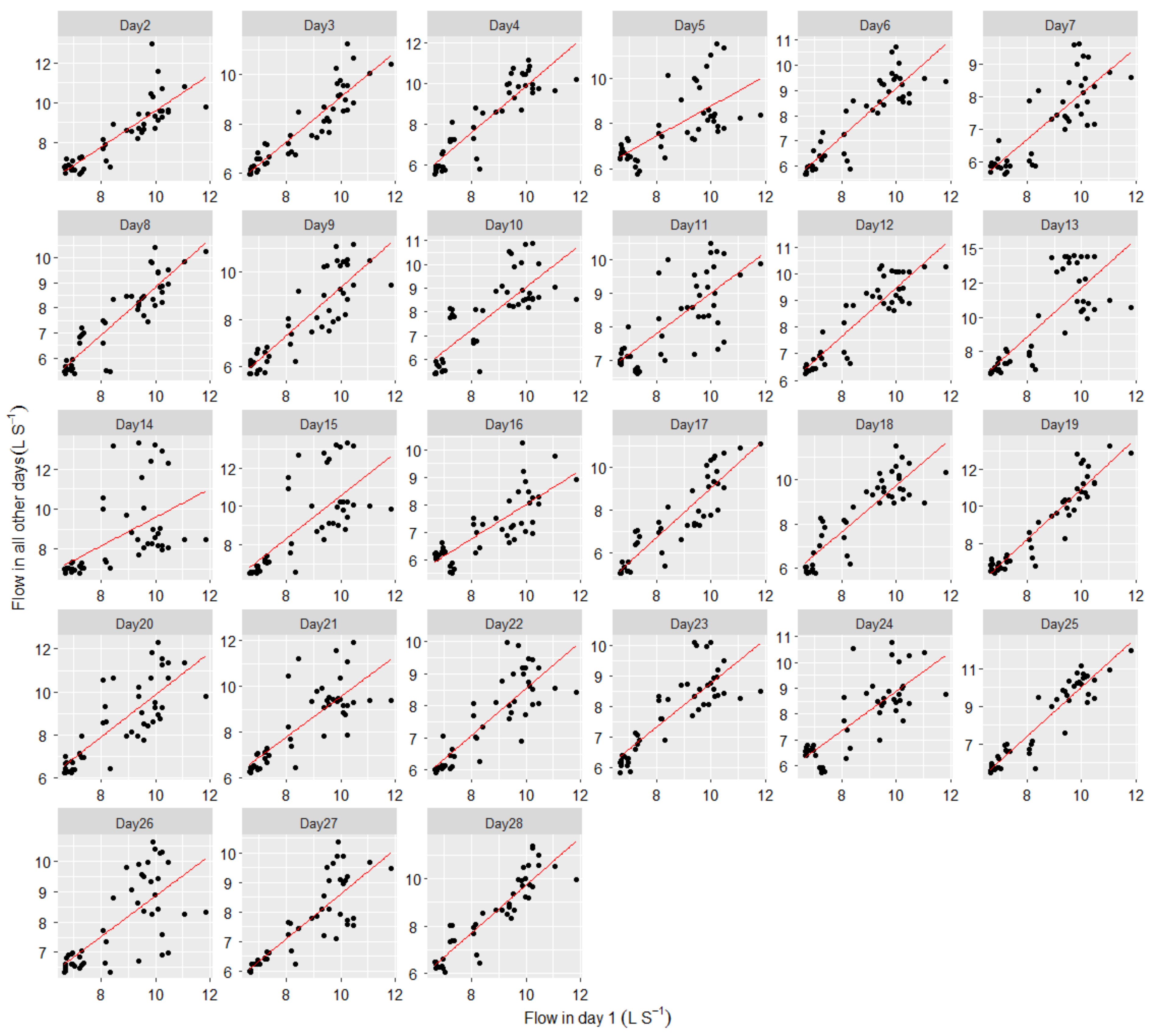
Further investigation was conducted to model the relationship between the flow patterns on different days. Figure 5 shows the plot of demand multipliers on the first day against the same on all other days during the study period. In the figure, it is evident that a linear relationship exists between the demand multipliers on different days. The trend lines of these linear models have an offset in the y-axis to the origin.
Hence, using the daily multiplication factor may not be adequate to represent their relationship. Therefore, the intercept term was also considered in modelling the demand pattern relationship. Both the slope and the intercept terms were considered as calibration parameters, and their values were searched through the calibration process that closely represents their relationship. This range of parameters related to demand modelling allows additional pathways for further reduction of the objective function during calibration. However, this increases the number of parameters to optimise, hence, increasing the solution space. Running the optimisation task in the HPC environment can effectively handle this kind of large problem. Non-linear functions were not considered as they introduce more parameters than linear functions, consequently, the problem size would also increase.
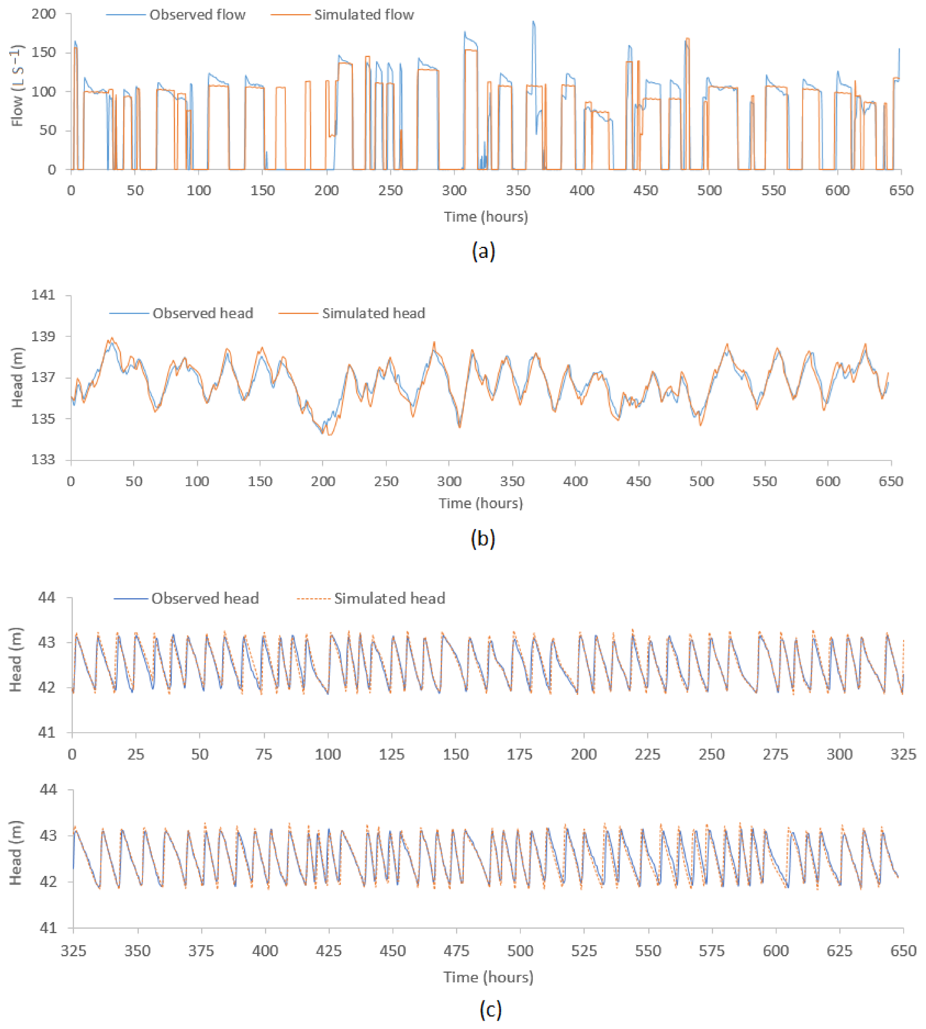
CMAES and SCE optimisation were run with different population sizes and a different number of complexes. It was found that increasing the number of complexes in the SCE optimisation considerably increased the number of model runs. The global search does not require any starting points as they perform the optimisation considering multiple start points. However, providing a set of initial values considerably decreases the number of model runs. Hence, the patterns identified through data analysis for residential demand multipliers and the typical values of commercial demand multipliers were used as the initial starting point for CMAES and SCE runs, respectively. For a local search using the GLMA algorithm, R codes were composed to generate random starting points within the upper and lower boundaries of the parameters. Several batch runs were performed with 28 local searches in each batch employing all 28 processors in a single HPC node. However, none of these GLMA-based searches seemed to proceed towards the global minima, while CMAES and SCE showed comparatively more reduction of the objective function. Figure 6 presents the observed and model-simulated time-series corresponding to the best objective function at three different locations in the TBK WDS: (a) flow at pump station 2 (PS2); (b) head at Binnies tank; (c) head at Meningie tank.
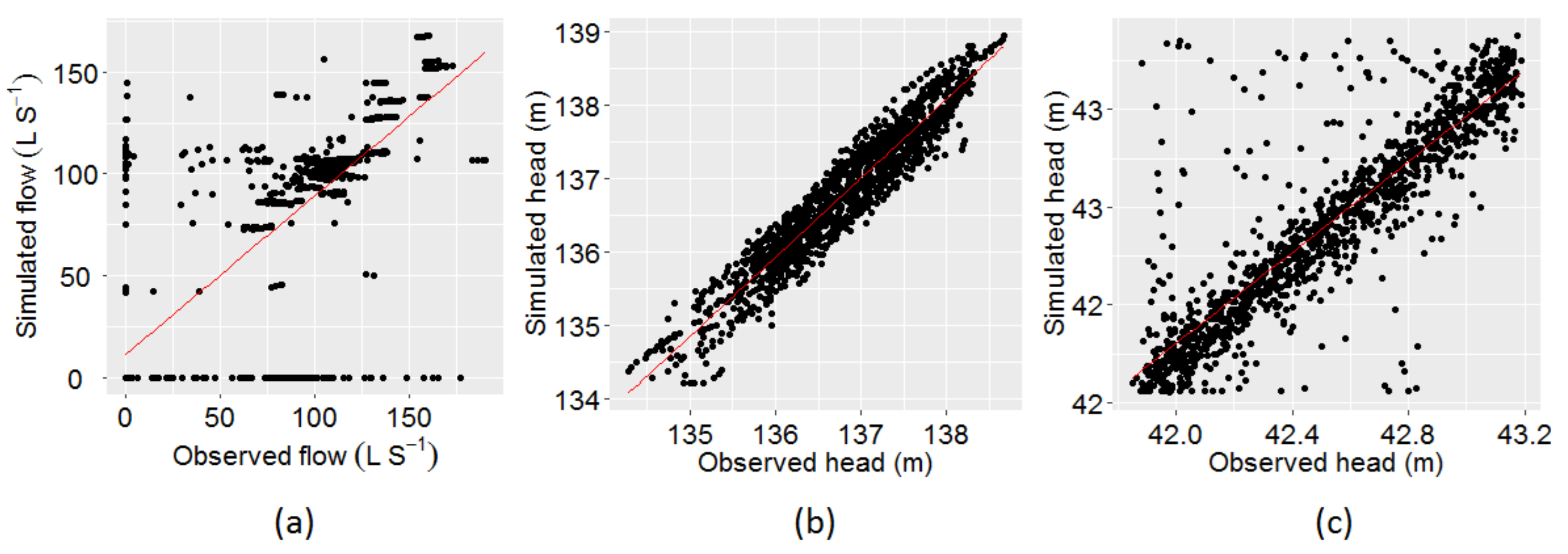
As can be seen in Figure 6, simulated time-series closely match with the observed time-series. However, Figure 6a shows that the simulated flow was steady while the pump was running but the actual observed flow was unsteady, indicating that the variable pump speed was poorly simulated by the model. Some studies have suggested simulating the variable pump speed by modifying the rotor speed using several rule-based controls [43]. This was not further explored in the current study considering the optimisation problem size as several additional parameters would have been needed to be included in the model to simulate the variable pump speed. Furthermore, the simulated flow between 160 to 190 h suggests that the pump was run twice, while the observed flow data shows zero flows during this period. The tank connected to the pump (Figure 6b) also indicates a rise of head twice between 160 to 190 h. This suggest that there could be possible SCADA outage or instrument failure during this period, hence, no data was recorded. Figure 7 presents the plot of observed vs model-simulated values at these locations. The correlation between the observed and the simulated flows at PS2 and heads at Binnies and Meningie tanks were 0.89, 0.96 and 0.88, respectively. The mean of the observed flow and heads at these locations were 57.12 L S−1, 136.77 m and 42.53 m, respectively, while the same obtained through model simulation were 54.71 L S−1, 136.78 m and 42.54 m, respectively. These statistics indicate that the observed data were reasonably reproduced.
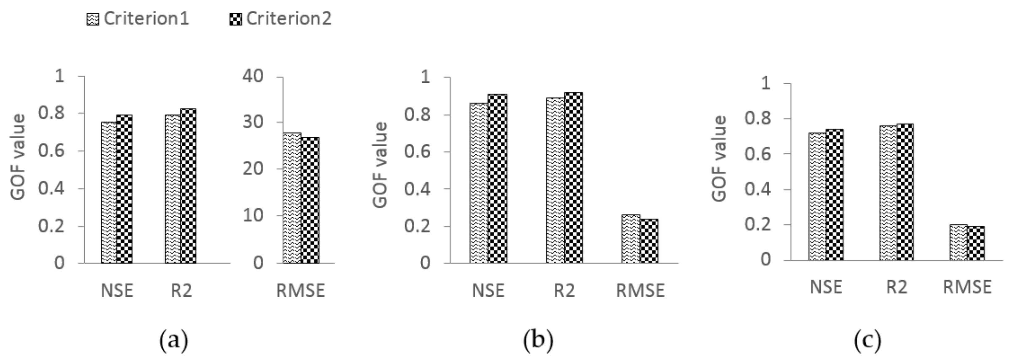
The modelling of variable demand patterns and the corresponding calibration performance was compared using two different criteria: (i) daily demand multiplication factors and (ii) a linear modelling approach. GOF tests were used to assess the fit between the observed and the model simulated values. The GOF statistics for both cases are presented in Figure 8 where an improved fit is evident under second criterion. The value of NSE, R2 and RMSE for the first criterion at PS2 were 0.73, 0.77 and 27.63, respectively, while for the second criterion they were 0.77, 0.80 and 26.80, respectively. Similarly, at Binnies tank, NSE, R2 and RMSE between the observed and simulated time-series were 0.86, 0.89 and 0.26, respectively, under criterion 1, while for criterion 2, they were 0.91, 0.92 and 0.24, respectively. On the other hand, at Meningie tank, the values of NSE, R2 and RMSE for criterion 1 were 0.72, 0.76 and 0.20, respectively, while for criterion 2 they were 0.74, 0.77 and 0.19, respectively. These statistics indicate that the proposed method to model the variable demand patterns can improve the fit between the observed and simulated time-series. Although the calibration performances under both criteria during the studied period do not differ much, incorporating the linear modelling parameters into the calibration process allows modelling of the demand patterns on days with a relatively flatter peak.
Both CMAES and SCE algorithms showed different levels of optimisation performance. Compared to CMAES, it took considerably longer to complete the optimisation process by the SCE algorithm. Up to five complexes and 90,000 runs were tried but the overall achievement was poorer than CMAES. Increasing the number of complexes may improve the performance of SCE optimisation. Likewise, for SCE algorithm settings, increasing the population size was found to improve the CMAES performance. Hence, both of the CMAES and SCE algorithms’ performances were found to be subjective, and they varied with many factors, including the algorithm runtime settings. Furthermore, no leakage analysis was performed in the current study. Modelling and including the emitter parameters to the calibration can ensure water loss through leakage is reasonably accounted for, which can further improve the overall calibration performance. Table 2 presents a summary of the calibration run information using the different optimisation algorithms.
4. Conclusions
This paper has incorporated a linear modelling approach into the calibration of the water distribution system hydraulic model that allows the modelling of variable demand patterns and obtaining a better calibration by fine tuning the linear modelling parameters. A large drinking water distribution system in South Australia was selected as a case study. EPANET was used to build up the hydraulic model, and the SCADA data were used to configure the initial states of the network. The analysis of flow data during the simulation period suggests an association between flow patterns on various days. The existing modelling technique of variable demand patterns that uses a single multiplication factor for each day can be further improved by using the linear modelling approach. For each day of the simulation period, the linear model parameters can have different values. Hence, they were optimised to capture the maximum variation of demand patterns. A global optimisation algorithm and local optimisation with multiple start points were used to find the optimum parameter values. Throughout the calibration process, the demand patterns for all days were generated using the linear modelling slope and intercept parameters, and they were combined together to create a time-series that was placed into the hydraulic model’s input file prior to each model run. Several software tools were incorporated together and their performance in running the whole calibration process was investigated in order. Out of the optimisation algorithms investigated, the covariance matrix adaptation evolution strategy showed a better performance compared to the shuffled complex evolution and the Gauss–Levenberg–Marquardt algorithm. The calibrated model showed a good agreement with the observed data. The correlation between the observed and simulated flow was 0.89 and between the observed and simulated tank heads at two different locations they were 0.96 and 0.88. However, a limitation of the proposed method is that by introducing additional parameters, the optimisation problem size, hence the solution space, is increased, which increases the number of model runs and the convergence time. This issue can be handled by running the optimisation task using a high performance parallel computing environment. Overall, this approach was found to improve the calibration of the water distribution system hydraulic model.
Author Contributions
Conceptualization, S.H., G.A.H., C.W.K.C. and D.C.; Data curation, S.H.; Formal analysis, S.H.; Funding acquisition, G.A.H., C.W.K.C. and D.C.; Investigation, S.H., G.A.H., C.W.K.C. and D.C.; Methodology, S.H., G.A.H., C.W.K.C. and D.C.; Resources, G.A.H., C.W.K.C. and D.C.; Software, S.H.; Supervision, G.A.H., C.W.K.C. and D.C.; Validation, S.H., G.A.H., C.W.K.C. and D.C.; Writing—original draft, S.H.; Writing—review and editing, G.A.H., C.W.K.C. and D.C. All authors have read and agreed to the published version of the manuscript.
Funding
The University of South Australia provided funding for this project through the postgraduate scholarship award scheme. Additional funding was provided by the South Australian Water Corporation through Water Research Australia (grant number 4535-17).
Acknowledgments
This project was a collaboration by the University of South Australia, Water Research Australia, the South Australian Water Corporation, TRILITY and DCM Process Control. We acknowledge all parties for their time and effort in the project. Special thanks to South Australian Water Corporation for their support by providing the necessary data.
Conflicts of Interest
The authors declare no conflict of interest.
References
- Peters, A.; Liang, B.; Tian, H.; Li, Z.; Doolan, C.; Vitanage, D.; Norris, H.; Simpson, K.; Wang, Y.; Chen, F. Data-driven water quality prediction in chloraminated systems. Water e-J. 2020, 5, 1–19. [Google Scholar] [CrossRef]
- Kara, S.; Karadirek, I.E.; Muhammetoglu, A.; Muhammetoglu, H. Hydraulic Modeling of a Water Distribution Network in a Tourism Area with Highly Varying Characteristics. Procedia Eng. 2016, 162, 521–529. [Google Scholar] [CrossRef] [Green Version]
- Ormsbee, L.E.; Lingireddy, S. Calibrating hydraulic network models. J. AWWA 1997, 89, 42–50. [Google Scholar] [CrossRef]
- Shen, H.; McBean, E. Hydraulic calibration for a small water distribution network. In Water Distribution Systems Analysis 2010; American Society of Civil Engineers: Reston, VA, USA, 2010; pp. 1545–1557. [Google Scholar]
- Alves, Z.; Muranho, J.; Albuquerque, T.; Ferreira, A. Water Distribution Network’s Modeling and Calibration. A Case Study based on Scarce Inventory Data. Procedia Eng. 2014, 70, 31–40. [Google Scholar] [CrossRef] [Green Version]
- Liong, S.-Y.; Atiquzzaman, M. Optimal design of water distribution network using shuffled complex evolution. J. Inst. Eng. 2004, 44, 93–107. [Google Scholar]
- Moosavian, N.; Jaefarzadeh, M.R. Hydraulic analysis of water distribution network using shuffled complex evolution. J. Fluids 2014, 2014, 979706. [Google Scholar] [CrossRef] [Green Version]
- Duan, Q.; Sorooshian, S.; Gupta, V.K. Optimal use of the SCE-UA global optimization method for calibrating watershed models. J. Hydrol. 1994, 158, 265–284. [Google Scholar] [CrossRef]
- Duan, Q.; Sorooshian, S.; Gupta, V. Effective and efficient global optimization for conceptual rainfall-runoff models. Water Resour. Res. 1992, 28, 1015–1031. [Google Scholar] [CrossRef]
- Hansen, N.; Ostermeier, A. Completely Derandomized Self-Adaptation in Evolution Strategies. Evol. Comput. 2001, 9, 159–195. [Google Scholar] [CrossRef]
- Hansen, N.; Kern, S. Evaluating the CMA Evolution Strategy on Multimodal Test Functions. In Parallel Problem Solving from Nature—PPSN VIII; Springer: Berlin/Heidelberg, Germany, 2004; pp. 282–291. [Google Scholar]
- Doherty, J. PEST: Model Independent Parameter Estimation—User Manual, 5th ed.; Watermark Numerical Computing: Brisbane, Australia, 2005. [Google Scholar]
- Khedr, A.; Tolson, B.; Ziemann, S. Water distribution system calibration: Manual versus optimization-based approach. Procedia Eng. 2015, 119, 725–733. [Google Scholar] [CrossRef] [Green Version]
- Zanfei, A.; Menapace, A.; Santopietro, S.; Righetti, M. Calibration Procedure for Water Distribution Systems: Comparison among Hydraulic Models. Water 2020, 12, 1421. [Google Scholar] [CrossRef]
- Do, N.C.; Simpson, A.R.; Deuerlein, J.W.; Piller, O. Calibration of Water Demand Multipliers in Water Distribution Systems Using Genetic Algorithms. J. Water Resour. Plan. Manag. 2016, 142, 04016044. [Google Scholar] [CrossRef]
- Do, N.C.; Simpson, A.R.; Deuerlein, J.W.; Piller, O. Particle Filter-Based Model for Online Estimation of Demand Multipliers in Water Distribution Systems under Uncertainty. J. Water Resour. Plan. Manag. 2017, 143, 04017065. [Google Scholar] [CrossRef] [Green Version]
- Letting, L.K.; Hamam, Y.; Abu-Mahfouz, A.M. Estimation of Water Demand in Water Distribution Systems Using Particle Swarm Optimization. Water 2017, 9, 593. [Google Scholar] [CrossRef] [Green Version]
- Elhay, S.; Simpson, A.R. Dealing with Zero Flows in Solving the Nonlinear Equations for Water Distribution Systems. J. Hydraul. Eng. 2011, 137, 1216–1224. [Google Scholar] [CrossRef] [Green Version]
- Farley, M. Leakage Management and Control: A Best Practice Training Manual; World Health Organization: Geneva, Switzerland, 2001. [Google Scholar]
- Ávila, C.A.M.; Sánchez-Romero, F.-J.; López-Jiménez, P.A.; Pérez-Sánchez, M. Leakage Management and Pipe System Efficiency: Its Influence in the Improvement of the Efficiency Indexes. Water 2021, 13, 1909. [Google Scholar] [CrossRef]
- García-Ávila, F.; Avilés-Añazco, A.; Ordoñez-Jara, J.; Guanuchi-Quezada, C.; Flores del Pino, L.; Ramos-Fernández, L. Pressure management for leakage reduction using pressure reducing valves. Case study in an Andean city. Alex. Eng. J. 2019, 58, 1313–1326. [Google Scholar] [CrossRef]
- Puust, R.; Kapelan, Z.; Savic, D.A.; Koppel, T. A review of methods for leakage management in pipe networks. Urban Water J. 2010, 7, 25–45. [Google Scholar] [CrossRef]
- Zyl, J.E.v.; Clayton, C.R.I. The effect of pressure on leakage in water distribution systems. Water Manag. 2007, 160, 109–114. [Google Scholar] [CrossRef]
- García, I.F.; Novara, D.; Mc Nabola, A. A Model for Selecting the Most Cost-Effective Pressure Control Device for More Sustainable Water Supply Networks. Water 2019, 11, 1297. [Google Scholar] [CrossRef] [Green Version]
- Karimov, A.; Molden, D.; Khamzina, T.; Platonov, A.; Ivanov, Y. A water accounting procedure to determine the water savings potential of the Fergana Valley. Agric. Water Manag. 2012, 108, 61–72. [Google Scholar] [CrossRef]
- Mercedes Garcia, A.V.; López-Jiménez, P.A.; Sánchez-Romero, F.-J.; Pérez-Sánchez, M. Objectives, Keys and Results in the Water Networks to Reach the Sustainable Development Goals. Water 2021, 13, 1268. [Google Scholar] [CrossRef]
- Dandy, G.; Roberts, A.; Hewitson, C.; Chrystie, P. Sustainability Objectives for the Optimization of Water Distribution Networks. In Water Distribution Systems Analysis Symposium 2006; American Society of Civil Engineers: Reston, VA, USA, 2008; pp. 1–11. [Google Scholar]
- Kang, D.; Lansey, K. Demand and Roughness Estimation in Water Distribution Systems. J. Water Resour. Plan. Manag. 2011, 137, 20–30. [Google Scholar] [CrossRef]
- Hossain, S.; Chow, C.W.K.; Hewa, G.A.; Cook, D.; Harris, M. Spectrophotometric Online Detection of Drinking Water Disinfectant: A Machine Learning Approach. Sensors 2020, 20, 6671. [Google Scholar] [CrossRef]
- Muranho, J.; Ferreira, A.; Sousa, J.; Gomes, A.; Marques, A.S. Convergence issues in the EPANET solver. Procedia Eng. 2015, 119, 700–709. [Google Scholar] [CrossRef] [Green Version]
- Rossman, L.A.; Woo, H.; Tryby, M.; Shang, F.; Janke, R.; Haxton, T. EPANET 2.2 User Manual; U.S. Environmental Protection Agency: Washington, DC, USA, 2020. [Google Scholar]
- Todini, E.; Pilati, S. A gradient method for the solution of looped pipe networks. In Computer Applications in Water Supply: Volume 1—System Analysis and Simulation; Coulbeck, B., Orr, C.H., Eds.; John Wiley & Sons: Hoboken, NJ, USA, 1988; pp. 1–20. [Google Scholar]
- Doherty, J.; Skahill, B.E. An advanced regularization methodology for use in watershed model calibration. J. Hydrol. 2006, 327, 564–577. [Google Scholar] [CrossRef]
- Hossain, S.; Hewa, G.A.; Wella-Hewage, S. A Comparison of Continuous and Event-Based Rainfall–Runoff (RR) Modelling Using EPA-SWMM. Water 2019, 11, 611. [Google Scholar] [CrossRef] [Green Version]
- R Core Team. R: A Language and Environment for Statistical Computing; R Core Team: Vienna, Austria, 2019. [Google Scholar]
- Nishida, K.; Akimoto, Y. PSA-CMA-ES: CMA-ES with population size adaptation. In Proceedings of the Genetic and Evolutionary Computation Conference, Kyoto, Japan, 15–19 July 2018; pp. 865–872. [Google Scholar]
- Auger, A.; Hansen, N. A restart CMA evolution strategy with increasing population size. In Proceedings of the 2005 IEEE Congress on Evolutionary Computation, Edinburgh, UK, 2–5 September 2005; Volume 1762, pp. 1769–1776. [Google Scholar]
- Kuczera, G. Efficient subspace probabilistic parameter optimization for catchment models. Water Resour. Res. 1997, 33, 177–185. [Google Scholar] [CrossRef]
- Lepot, M.; Aubin, J.-B.; Clemens, F.H.L.R. Interpolation in Time Series: An Introductive Overview of Existing Methods, Their Performance Criteria and Uncertainty Assessment. Water 2017, 9, 796. [Google Scholar] [CrossRef] [Green Version]
- Moriasi, D.; Arnold, J.; van Liew, M.W.; Bingner, R.; Harmel, R.D.; Veith, T.L. Model Evaluation Guidelines for Systematic Quantification of Accuracy in Watershed Simulations. Trans. ASABE 2007, 50, 885–900. [Google Scholar] [CrossRef]
- Pérez-Sánchez, M.; Sánchez-Romero, F.J.; Ramos, H.M.; López-Jiménez, P.A. Optimization Strategy for Improving the Energy Efficiency of Irrigation Systems by Micro Hydropower: Practical Application. Water 2017, 9, 799. [Google Scholar] [CrossRef] [Green Version]
- Pérez-Sánchez, M.; Sánchez-Romero, F.J.; Ramos, H.M.; López-Jiménez, P.A. Calibrating a flow model in an irrigation network: Case study in Alicante, Spain. Span. J. Agric. Res. 2017, 15, 1202. [Google Scholar] [CrossRef]
- Georgescu, A.-M.; Georgescu, S.-C.; Cosoiu, C.I.; Hasegan, L.; Anton, A.; Bucur, D.M. EPANET Simulation of Control Methods for Centrifugal Pumps Operating under Variable System Demand. Procedia Eng. 2015, 119, 1012–1019. [Google Scholar] [CrossRef] [Green Version]
Figure 1.
Layout of the Tailem Bend–Keith (TBK) drinking water distribution system.

Figure 2.
Node-link representation in EPANET.

Figure 3.
Flowchart of the calibration procedure.

Figure 4.
(a) Flow pattern on different days during the simulation period and (b) estimated average demand multipliers from flow patterns.
Figure 4.
(a) Flow pattern on different days during the simulation period and (b) estimated average demand multipliers from flow patterns.

Figure 5.
Plot of day 1 flows vs flows on sequential days.

Figure 6.
Plot of observed vs model simulated values (a) flow at PS2 (b) head at Binnies tank and (c) head at Meningie tank.
Figure 6.
Plot of observed vs model simulated values (a) flow at PS2 (b) head at Binnies tank and (c) head at Meningie tank.

Figure 7.
Plot of observed vs model-simulated values (a) flow at PS2 (b) head at Binnies tank and (c) head at Meningie tank.
Figure 7.
Plot of observed vs model-simulated values (a) flow at PS2 (b) head at Binnies tank and (c) head at Meningie tank.

Figure 8.
Comparison of calibration performance while modelling the variable demand patterns using daily multiplication factors (criterion 1) and linear models (criterion 2) (a) GOF for PS2 (b) GOF for Binnies tank and (c) GOF for Meningie tank.
Figure 8.
Comparison of calibration performance while modelling the variable demand patterns using daily multiplication factors (criterion 1) and linear models (criterion 2) (a) GOF for PS2 (b) GOF for Binnies tank and (c) GOF for Meningie tank.


Table 1.
Selected parameters to calibrate the hydraulic model.
| Parameter Group | No. of Parameters | Group Range |
|---|---|---|
| Pipe roughness | 9 | 87–165 |
| Pump settings/rotor speed | 42 | 0.80–1.33 |
| Time-based controls for pump operation | 83 | 2–644 |
| Morning and evening peak shifting | 56 | ±3 |
| Linear model slope parameter | 28 | 0.70–1.40 |
| Linear model Intercept parameter | 28 | 0.00–0.30 |
Table 2.
Calibration run summary using different optimisation algorithms.
| Optimisation Algorithm | Algorithm Type | Number of Model Runs | Elapsed Time | % Reduction of Objective Function |
|---|---|---|---|---|
| CMAES | Global search | 14,338 | 16 h using 28 processors | 29 |
| SCE | Global search | 90,000 | 9 days and 16 h using 5 processors | 22 |
| GLMA | Local search | 3196 | 1 day and 15 h using single processer | 19 |
Publisher’s Note: MDPI stays neutral with regard to jurisdictional claims in published maps and institutional affiliations. |
© 2021 by the authors. Licensee MDPI, Basel, Switzerland. This article is an open access article distributed under the terms and conditions of the Creative Commons Attribution (CC BY) license (https://creativecommons.org/licenses/by/4.0/).
Share and Cite
MDPI and ACS Style
Hossain, S.; Hewa, G.A.; Chow, C.W.K.; Cook, D. Modelling and Incorporating the Variable Demand Patterns to the Calibration of Water Distribution System Hydraulic Model. Water 2021, 13, 2890. https://doi.org/10.3390/w13202890
AMA Style
Hossain S, Hewa GA, Chow CWK, Cook D. Modelling and Incorporating the Variable Demand Patterns to the Calibration of Water Distribution System Hydraulic Model. Water. 2021; 13(20):2890. https://doi.org/10.3390/w13202890
Chicago/Turabian StyleHossain, Sharif, Guna A. Hewa, Christopher W. K. Chow, and David Cook. 2021. "Modelling and Incorporating the Variable Demand Patterns to the Calibration of Water Distribution System Hydraulic Model" Water 13, no. 20: 2890. https://doi.org/10.3390/w13202890
Note that from the first issue of 2016, this journal uses article numbers instead of page numbers. See further details here.