Identification of Natural and Anthropogenic Geochemical Processes Determining the Groundwater Quality in Port del Comte High Mountain Karst Aquifer (SE, Pyrenees)

Abstract

The Port del Comte Massif (SE, Pyrenees) contains one of the most important vulnerable and strategic karst aquifers for supplying freshwater to the city of Barcelona (Spain). It is a fragile system, whose possible environmental impact is highly conditioned by land use. To improve the hydrogeological knowledge of the system, between September 2013 and October 2015, a detailed fieldwork was carried out for the revision of the geological model, the inventory of water points, and the in situ physico-chemical characterization on major elements and isotopes of up to a total of 43 springs, as well as precipitation water. This paper focuses on the characterization of the geochemical processes that allow explanation of the observed chemical variability of groundwater drained by the pristine aquifer system to determine the origin of salinity. The results show that the main process is the dissolution of calcite and dolomite, followed by gypsum and halite, and a minor cation exchange-like process. Sulfur and oxygen isotopes from dissolved sulfate in the studied springs point out a geogenic origin related to the dissolution of gypsum from Triassic and Tertiary materials, and that the contribution from anthropogenic sources, like fertilizers, is lower. Nitrate in groundwater is not an important issue, with a few localized cases related with agricultural activities. The multidisciplinary approach has allowed the development of a consistent hydrogeological conceptual model of the functioning of the aquifer system, which can be replicated in other places to understand the geogenic character of the hydrogeochemistry.

1. Introduction

High mountain karst aquifers are strategic freshwater reservoirs to maintain dependent ecosystems downstream, many of which are in semiarid zones. Globally, 68.9% of all the surface exposures of carbonate rocks occur in hills and mountain areas. Roughly, 20–25% of the world’s population depends directly or indirectly on water supplies from karst aquifers [1]. Given the relevance, it is essential to characterize such mountain karst aquifers and protect them to avoid undesirable quality issues in the stored water resources, because karst aquifers have been shown to be very vulnerable, especially to pollution, given their inner structure, hydrogeological behavior, and limited self-depuration capacity [2]. This is true especially when these karst aquifers are unconfined and the focused recharge flows through the most conductive karst features. This facilitates the widespread rapid incorporation and transport of pollutants to groundwater [3]. Such threating process might even be highlighted in the framework of climate change, mainly through the possible warming trends devised by the Intergovernmental Panel on Climate Change [4]. The expected increasing temperatures will reduce solid atmospheric precipitation and hence the snow cover duration in the mountain areas. This will drive the aquifer-dominant recharge process to migrate from spatial diffuse to a focused one [5], while exposing the aquifer to eventual surface contamination by anthropogenic activities for longer [6].

Mountain karst aquifers developed in carbonate materials are usually complex systems that may show a distinctive hydrochemical response depending on the physicochemical processes controlling the water–rock interactions. During the transit of groundwater (GW) from the recharge areas to the discharge zones, different hydrochemical processes may take place, including dissolution-precipitation reactions associated with carbonate materials [7,8], dissolution processes often associated with evaporite lithologies (e.g., gypsum, anhydrite, halite) [9,10], and even cation release/retention processes associated with shales [11]. The existence and role of these hydrochemical processes depend strongly on the geological settings of the mountain range hosting the aquifer, which are typically complex due to the orogenic processes driving the range uplift. Such hydrochemical processes along with the heterogeneity in the inner karst structure make characterizing the behavior of the associated aquifer system difficult. To this end, it is convenient to adopt a multidisciplinary approach [12], considering the hydrodynamic behavior and analyzing the physico-chemical and isotopic characteristics of groundwater (GW) throughout the aquifer [7,13,14,15,16], using both environmental and chemical tracers [17,18,19], applying data analysis techniques [20,21,22], conducting geophysical prospection [23], and/or applying hydrodynamic and hydrogeochemical and isotopic modeling tools [24,25,26,27,28,29].

The Port del Comte Massif (PCM) is a Mediterranean mountain karst aquifer located in the complex geotectonic zone of the south-eastern Pyrenean region [30,31]. The aquifer discharges through a series of springs with typically low flow rates (<1 L/s) [29]. Nevertheless, with a mean annual discharge of 7.5 hm³/year, the spring Fonts del Cardener stands out. This spring tributes downstream to the Llobregat River and amounts to 7% of the mean annual water use of Barcelona [32]. Several authors have investigated the PCM karst aquifer from different perspectives, including the delineation of the catchment zone associated with the main springs of PCM by building a 3-D geological model of the massif [33], the characterization of the hydrodynamic behavior of such springs and their associated GW transit time distributions [29], and the definition of natural background levels (NBLs) for NO₃, SO₄, and Cl in the aquifer, as NBLs are especially important to detect GW contamination from anthropic activities in PCM, given that the aquifer system presents a high intrinsic vulnerability [34].

Despite the PCM being a strategic freshwater resource, there is not a thorough hydrogeochemical characterization of the aquifer. There are only scarce attempts centered in the SW part of the massif [35,36,37]. It is well known that mountain karst aquifers are vulnerable to climate change. The increasing warming trends impact directly on the snowpack cover formation, the corresponding snowmelt infiltration, and hence aquifer recharge. These effects have been predicted in well-known high mountain karst systems, such as the Hochifen–Gottesacker system in the Northern Alps [38] and the aquifer system of Sierra de las Nieves [39], with the latter being a privileged unparalleled observatory of the early impact of climate change in continental Europe since it is the southernmost high mountain karst system of the Iberian Peninsula. Moreover, [6] simulated the impact of climate change scenarios in the PCM at the end of the 21st century, considering an increase in temperature of up to +3.1 °C and a reduction of the snow cover of up to 76% with respect to the current conditions. A decrease in the snow cover exposes the karst system to external pollutants for longer, which is an issue, because the high hydraulic conductivity and limited self-depuration capacity of such aquifers make them especially vulnerable to pollution [2].

The aim of this work is to point out the geogenic origin of solutes as well as possible anthropogenic contributions driving the hydrogeochemical composition of GW in a pristine rural karst system to form a comprehensive picture of the hydrogeochemical behavior of this vulnerable type of aquifer in order to prevent the effect of changes due to future scenarios for global change.

2. The Study Area

2.1. Geographical and Climatological Settings

The PCM is approximately 100 km north of Barcelona (Spain), in the south of the eastern Pyrenees (Figure 1). The elevation of the mountainous massif ranges from 900 m a.s.l. to 2383 m a.s.l. at the ‘Padró dels Quatre Batlles’ peak. The study area covers an extension of about 110 km². The NW and SW part of the massif drain to the Segre River basin, whereas the eastern and southern parts drain to the Cardener river. The main source of this last river is the Fonts del Cardener spring (M-22, Figure 1). The area is covered by forest (63.9%) and mountain meadows (21.1%), which include one alpine ski resort and one cross-country (Nordic) ski resort, areas without soil and vegetation (11.5%), agricultural cultivation areas (1.5%), and the rest corresponding to residential zones (0.5%) [29]. From a climatological point of view, and according to the Köppen-Geiger classification system [40], the study area is characterized by a cold climate without a dry season and with a temperate summer. Within the study area, there are two meteorological stations located at 2315 m a.s.l. (SMC) and 1800 m a.s.l. (AEMET). For the period 2005 to 2019, the average annual precipitation, temperature, and potential evapotranspiration (Hargreaves) measured at the SMC station are 1055 mm, 3.24 °C, and 525 mm, respectively. During 3 to 4 months in the winter, depending on the year, the snow cover is above 1800 m a.s.l. The infiltration of the snowmelt during the spring season generates the main contribution to aquifer recharge in the PCM [29]. The massif presents a characteristic karst pattern in the upper part, which appears in the form of sinkholes and karren fields that allows a fast infiltration of the meteoric waters and prevents large surface runoff events.

2.2. Geology and Hydrogeology Setting

From the geological point of view, the PCM constitutes an independent thrust sheet limited by other thrusts with complex structural relationships (Figure 1). Internally, the massif presents a set of folds (anticlines and synclines) and some faults. The folds have a characteristic NE-SW direction parallel to the NW boundary of the thrust sheet [31]. Stratigraphically, the massif contains materials from the Triassic (Muschelkalk limestones and Keuper evaporites), the Cretaceous (limestones, calcarenites, shales), and the Paleogene from the Eocene to the Oligocene (karstified limestones with dolostones, sandstones, and marls). The Jurassic carbonates only outcrops in the NW part of the study area. The massif has a total thickness exceeding 1300 m. From the geomorphological perspective, the PCM is characterized by presenting a rounded or flat relief in the highest part, where no vegetation cover is present and almost without any type of soil development exists. The rest of the massif is covered by mountain meadows and forests, with little thin soil. The area most affected by karstification becomes visible progressively, from 1950 m a.s.l. to the top.

Hydrogeologically, the PCM can be considered an independent unit and a multi-aquifer system. The Lower Eocene fissured and karstified limestones and dolostones form the main aquifer. It constitutes one of the most important high mountain karst aquifers (HMKA) of the Catalan Pyrenees. The other aquifers and aquitards in the study zone are related to the Cretaceous limestone formations, Triassic limestone and evaporites, other Paleogene conglomerates and sandstones, and small local quaternary aquifers (draining small areas) located at low or medium elevations. The Garumnian materials (Upper Cretaceous-Lower Paleogene), composed of shales, marls, and multicolored clay deposits (geological unit 5 in Figure 1), constitute a low permeability layer that acts as a lower impervious limit for both the Tertiary materials and the main karst aquifer. In addition, the geological structure of the system strongly influences the location and hydrodynamical behavior of the springs and their geochemical fingerprint.

Although many high mountain karst systems play a strategic role in terms of availability of underground water resources, such as the case of PCM [29], frequently they are not sufficiently known because the conventional hydrogeological investigation techniques are often difficult to be applied given the complicated access and harsh working conditions typically existing in high mountain zones [42,43,44,45,46].

From a hydrological point of view, there are relevant processes, such as the aquifer recharge or the mean transit time, that need to be characterized to correctly manage the water resources generated in such alpine groundwater systems. Spring hydrograph analysis and the use of environmental tracer methods allow the characterization of aquifer recharge and discharge processes, assessing spring vulnerability, as well as estimating the available water resources [47,48,49,50]. Rainfall-runoff hydrological models are useful to simulate the behavior of such complex mountain karst systems. Such models can be broadly categorized into lumped, semi-distributed, and fully-distributed models [51]. Semi-distributed and lumped parameter models (LPMs) are often used to simulate the behavior of high mountain aquifer systems, because they do not require a detailed hydrological knowledge of the physical system, and therefore, they are specially well suited when the hydrogeological systems are poorly characterized. Additionally, the stable isotopes of water (δ¹⁸O and δ²H) in precipitation have proved to be good environmental tracers for investigating the dynamics of such hydrological systems karst systems [52]. These tracers enter the system as recharge, migrate downslope exploring the entire hydrological system, and leave the karst aquifer through the springs discharge. In the case of PCM, [29] presents a hydrogeological characterization of the aquifer system response that includes:

(1)

The hydrodynamic behavior of the system, simulating the system response with a set of semi-distributed rainfall-runoff HBV models [53,54], while taking into account the elevation dependences of both the hydrometeorological variables (e.g., precipitation and temperature) and the related processes (e.g., snow accumulation and ablation). The estimated groundwater storage capacity of the system is 35.2 hm³, and the mean annual groundwater discharge is 15.4 hm³; and

(2)

The estimation of the mean transit times corresponding to the main springs draining the aquifer system. This is done by using a set of LPMs models [55] to simulate the environmental tracers’ content evolution in groundwater. The LPMs were implemented for the most important karst springs of the PCM systems, i.e., the four ‘regional springs’ named as M-22, M-25, M-31, and M-43 in Figure 1. The results indicate that the PCM karst system presents a relatively short mean transit time (~2.25 year). This result is relevant if the hydrological high conductive features existing in the karst system are taken into account, which may favor a fast contaminant migration from the recharge to the discharge areas in the case of eventual surface spills of contaminants.

In the framework of the ‘GeoERA Resources of groundwater harmonized at cross-border and pan-European scale (RESOURCE) Project’ (2018–2021) funded from the European Union’s Horizon 2020 research and innovation programme, the PCM karst aquifer was incorporated as a pilot case study among others across Europe [56]. In this framework, a well-known hydrodynamic typology classification method proposed by Mangin (1975) is applied [57], which is based on a recession curve analysis of the spring hydrograph. The method describes the hydrodynamic behavior of a karst system as a function of two indices, k and i, defining the extent of the karst phreatic zone and characterizing the infiltration conditions, respectively. In the case of spring M-22, and for a diagram k vs. i [57], the indices lie in the k < 0.5 and i > 0.5 domain, thus indicating a complex, large karst system, made up of several sub-systems. This result is consistent with those obtained for other important karst springs in the Pyrenees, such as Fonts del Llobregat springs [58], which are one of the main groundwater resource for the Barcelona metropolitan area.

This manuscript presents the work done to characterize the PCM system from the hydrogeochemical point of view. In this sense, several geochemical fieldworks were carried out on 43 springs during the period September 2013–October 2015. The 43 springs were grouped from a geochemical point of view [59] applying an approach based on a the Gaussian mixture model (GMM) [60], obtaining four groups (Figure 2). GMM is a ‘soft’ model-based clustering method that avoids the degree of subjectivity assumed by the classical ‘hard’—or heuristic-based—algorithms (e.g., k-means, hierarchical clustering) [61] to determine the relevant number of clusters. Following [59], the four spring clusters found in PCM can be summarized as:

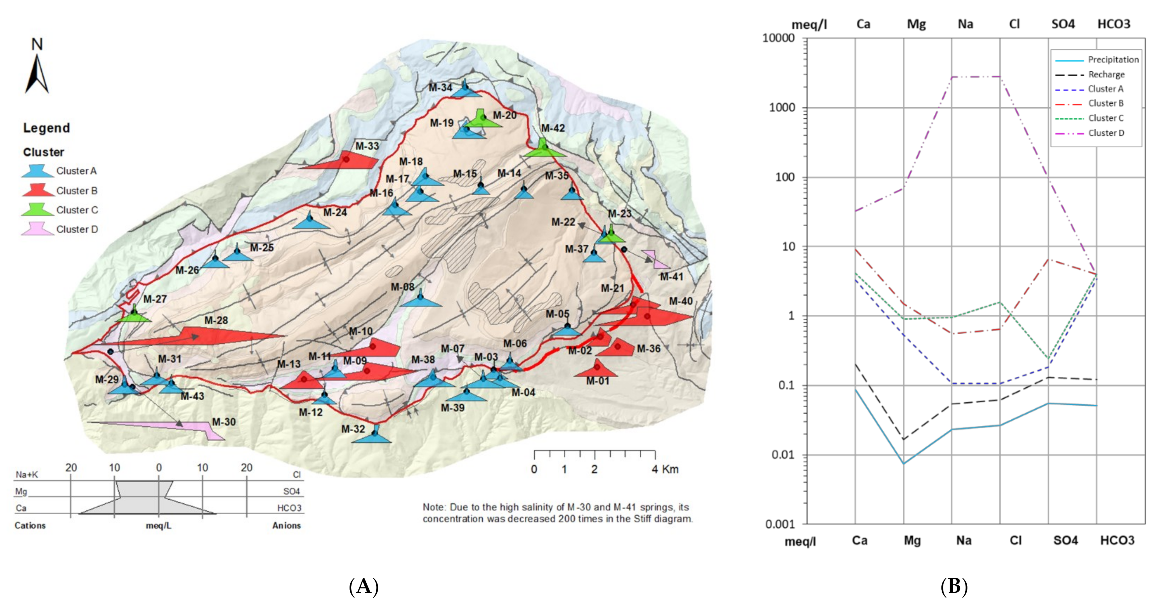
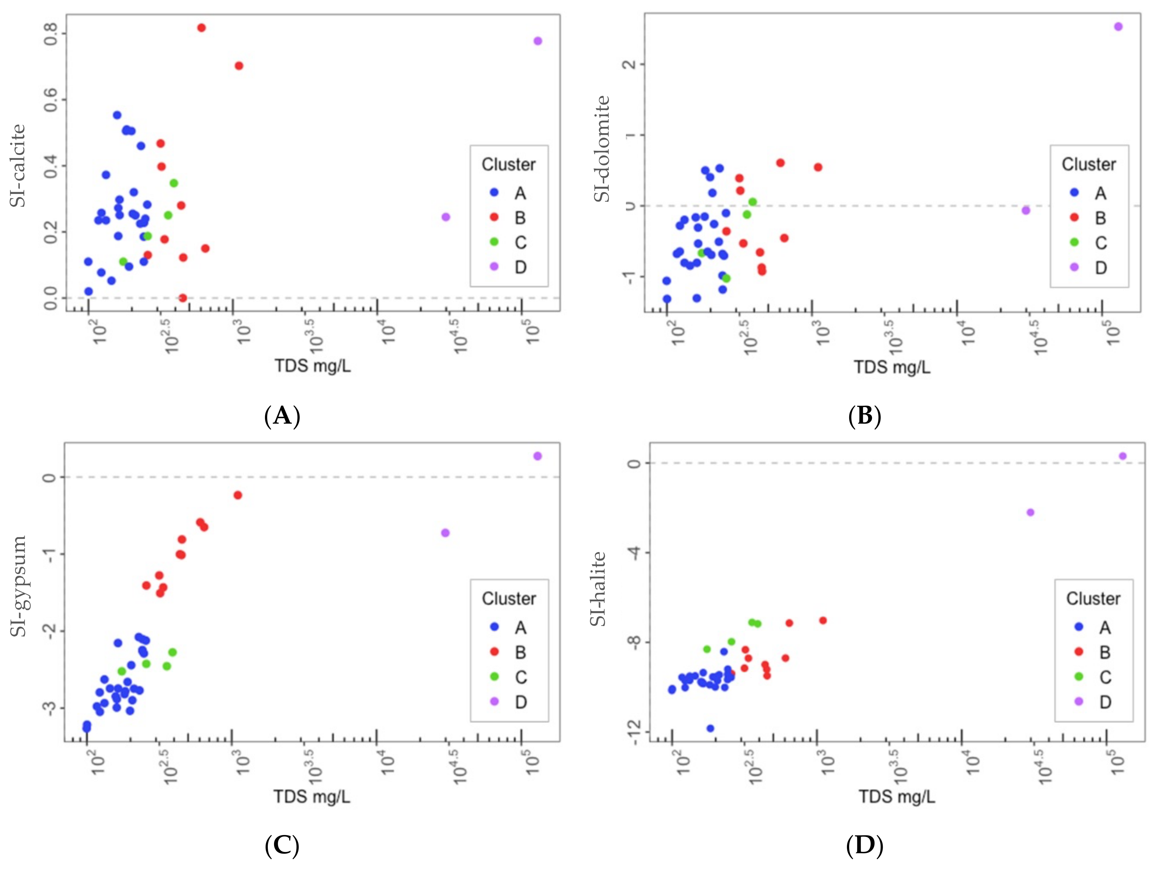
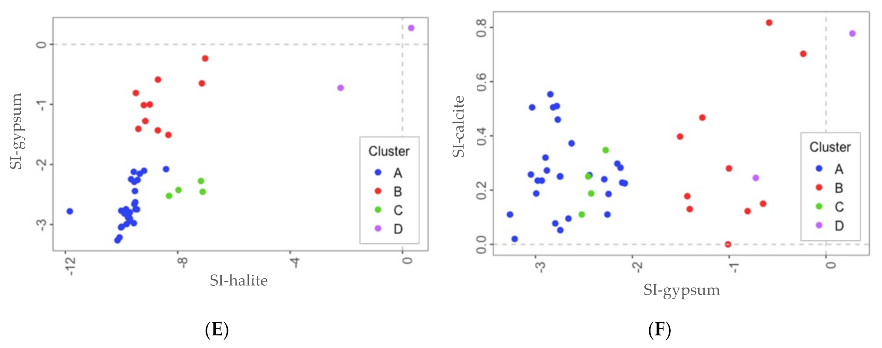
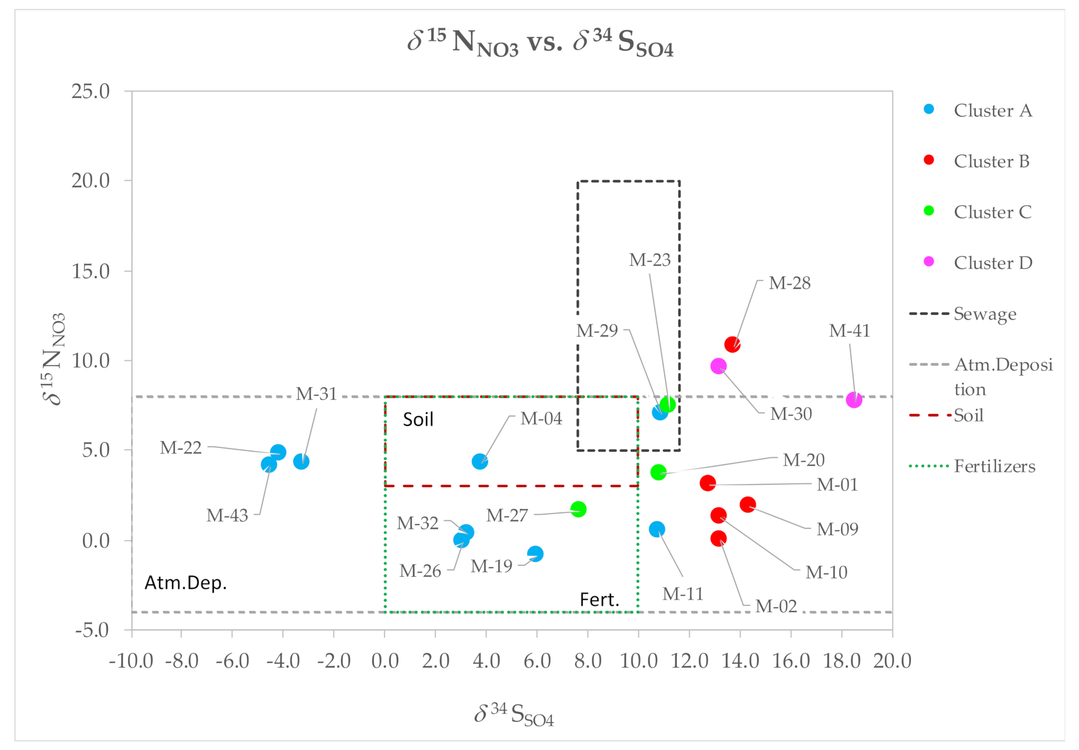
• Cluster A: 27 springs characterized by low mineralization and dominated by slightly alkaline Ca–HCO₃ water type, which is associated with the Eocene carbonate materials conforming the main aquifer of PCM.
• Cluster B: 10 springs that include different types of water from Ca–HCO₃ to Ca–HCO₃–SO₄, Ca–SO₄–HCO₃, and Ca–SO₄, which are characterized by moderate mineralization. These springs are located both inside and outside the structural limits of the PCM trust sheet. The springs located inside the limits are mainly found in materials from the Cretaceous and Triassic (Keuper) that outcrop in the area. These materials underlie the main aquifer of the massif (the Eocene karst carbonate system). In the southeastern part of the study zone, there are five springs related to sediments with a high content of tertiary gypsum from the Eocene-Oligocene Beuda’s gypsum Formation, pinched out within the South Pyrenees thrust fault in the front SE of the PCM.
• Cluster C: 4 springs with water types of Ca–HCO₃ and Ca–HCO₃–Cl. Three of these springs are located at the boundaries of the PCM sheet.
• Cluster D: corresponds to two salty springs with Na–Cl facies that are in the eastern and western limits of the PCM thrust sheet, respectively. They are characterized by remarkably high mineralization and are saturated relative to gypsum.

According to Herms et al. (2019) [29], the recharge of the main aquifer of the PCM is produced by diffuse infiltration of precipitation-rainfall and snowmelt, but it is also concentrated through the well-developed karstic elements, mostly situated at the top of the massif. The infiltrated water flows vertically through the unsaturated zone, which may be thicker than 1000 m, towards the saturated zone of the aquifer. GW discharges through a large network of springs. In the framework of this work, more than 100 springs have been identified in the study zone. Most of them discharge local sub-surface waters with low flow rates ranging between <0.1 L/s and 10 L/s. There are four ‘regional’ springs (M-22, M-25, M-31, and M-43; Figure 1) with mean flow rates from 1 L/s to 900 L/s, whose recharge areas are at medium to high elevation areas. Springs M-22 and M-25 discharge through Quaternary deposits overlying the Lower Eocene limestones, M-31 discharge directly through the limestone outcrops, and M-43 through well-developed karstic conduits affecting the conglomeratic materials of the Ebro Basin (the southern foreland basin of the Pyrenees), which are located just at the southern border of the PCM mantle. There are also some GW diffuse discharge zones, especially in the northern sector of the PCM. The regional water table main aquifer is located at elevations between 1000 and 1100 m a.s.l. [29].

3. Materials and Methods

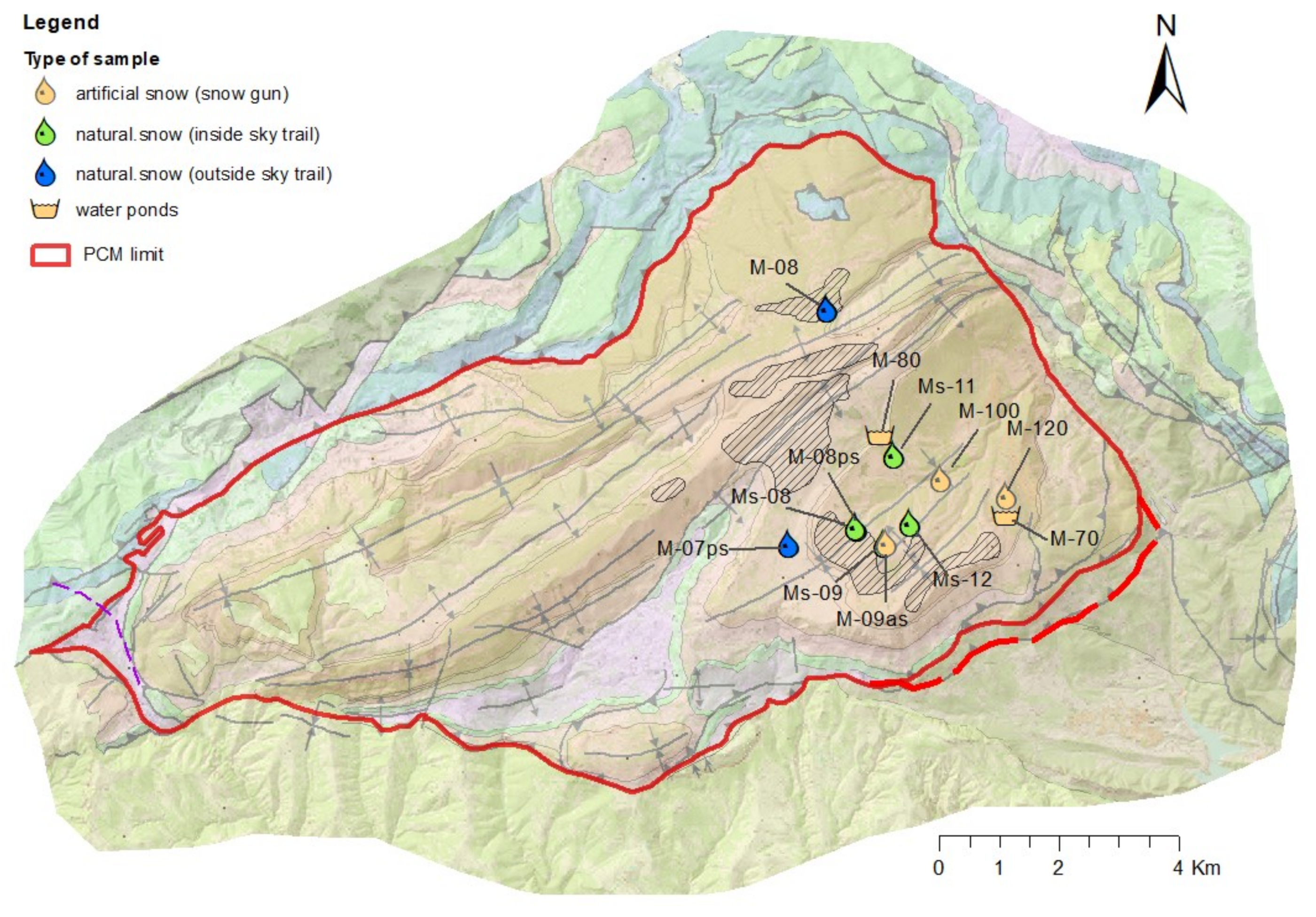
3.1. Field Measurements, Sampling, and Laboratory Analysis

A total of 43 springs (Figure 2A) were monitored in this research for the period from September 2013–October 2015, in which the springs were sampled twice per year (i.e., before snowfall in October and after snowmelt in April). Additionally, springs M-04, M-20, M-22, M-25, M-31, and M-43 were regularly sampled more frequently, every three to four weeks, along the same sampling period. In every case, the “in situ” physico-chemical parameters (pH, EC, T, redox, alkalinity, TDS) were measured. A total of 288 GW samples were obtained.

Table A1. Summary of water sample types and analysis done in the research project.

Type of Sample	Number of Control Points	Total Field Campaigns	Total Number of Samples	Number of Analysis with Major Ions	Number of Analysis with Trace Metals	Total Number Analysis Stable Isotopes of δ2HH2O, δ18O	Total Number Analysis Stable Isotopes of δ34S, δ18OSO42-	Total Number Analysis Stable Isotopes of δ15N, δ18ONO3-
Pluviometers (quarterly)	8	9	71	-	-	71	-	-
Spring samples	-	-	288	288	285	283	209	72
Springs (biannually)	40/43	4	-	138	136	134	88	42
Spring (monthly)	6	25	-	150	149	149	121	30
Snow samples			10	10	10	10	1	-
Natural snow	10	-	-	7	7	7	-	-
Artificial snow	3	-	-	3	3	3	1	-
Water ponds (artificial snow production)	2	-	2	2	2	-	-	-
		Total	371

in Appendix A summarizes the details of the GW sampling campaigns conducted in this work. Table A1,

Table A2. Chemical characteristics of major constituents for the 43 water springs (median values for the whole campaigns carried out from September 2013–October 2015).

ID	Num. Samples	Water Type	Cluster	GU	EC [μS/cm]	TDS [ppm]	pH	T [ºC]	Ca [ppm]	Mg [ppm]	Na [ppm]	K [ppm]	HCO3 [ppm]	Cl [ppm]	NO3 [ppm]	SO4 [ppm]
M-03	4	Ca-HCO3	A	PEalb	306.25	161.00	7.8	11.4	63.75	2.05	2.53	1.93	190.96	3.75	3.83	4.38
M-04	25	Ca-HCO3	A	POcgs	470.04	241.68	7.4	10.2	94.84	6.35	2.16	2.60	291.00	4.32	3.88	16.13
M-05	4	Ca-HCO3	A	Qpe	307.00	160.75	7.7	10.1	69.25	1.10	2.15	0.50	198.48	2.80	3.92	3.14
M-06	4	Ca-HCO3	A	KMgp	251.00	132.25	8.1	7.8	54.25	5.18	2.83	1.18	170.68	5.67	3.36	8.82
M-07	4	Ca-HCO3	A	POcgs	461.50	241.75	7.3	9.7	102.25	4.90	3.53	0.88	297.37	5.56	2.20	14.10
M-08	4	Ca-HCO3	A	KMgp	384.25	202.50	7.6	5.5	86.50	4.45	3.28	0.85	264.86	4.24	2.01	10.03
M-11	4	Ca-HCO3	A	KMca	312.75	164.00	8.0	10.7	59.25	5.50	3.78	0.65	162.11	4.16	10.84	25.35
M-12	4	Ca-HCO3	A	KMgp	252.00	132.25	7.9	8.5	54.50	2.35	1.70	0.58	167.31	4.29	1.88	4.19
M-14	4	Ca-HCO3	A	PPEc	190.75	100.25	8.0	5.8	44.75	1.85	1.43	0.48	119.61	2.55	5.48	2.62
M-15	3	Ca-HCO3	A	PEci	186.67	99.67	8.2	6.0	37.67	1.83	1.53	0.53	109.90	2.87	7.35	2.49
M-16	1	Ca-HCO3	A	PEci	306.00	184.00	8.0	13.4	60.00	12.00	1.00	0.80	221.00	2.50	0.50	6.30
M-17	2	Ca-HCO3	A	PEci	361.50	198.50	8.0	7.0	67.00	14.50	1.30	1.00	251.50	2.75	6.99	3.29
M-18	1	Ca-HCO3	A	PEci	385.00	231.00	7.9	11.9	64.00	18.00	1.70	3.80	253.00	2.50	8.30	6.40
M-19	4	Ca-HCO3	A	TJcd	392.00	206.00	7.8	7.4	63.25	18.75	1.85	0.73	258.30	4.43	5.62	4.60
M-22	25	Ca-HCO3	A	Qvl	241.04	122.71	7.9	7.4	44.64	6.14	1.63	0.49	147.94	5.35	3.19	7.14
M-24	4	Ca-HCO3	A	PPEc	402.50	211.50	7.6	8.2	77.50	11.00	3.18	1.08	269.94	6.59	3.00	5.45
M-25	25	Ca-HCO3	A	KMgp	323.76	164.32	7.8	8.0	65.84	5.03	1.75	0.59	210.24	3.36	2.54	5.87
M-26	3	Ca-HCO3	A	KMca	296.33	158.00	8.1	10.5	63.00	2.50	2.30	0.53	185.50	2.97	2.90	4.76
M-29	4	Ca-HCO3	A	Qpe	436.00	228.25	7.7	10.2	76.50	6.43	8.15	1.70	218.59	16.82	8.86	27.32
M-31	25	Ca-HCO3	A	PPEc	353.80	182.12	7.9	8.6	75.52	4.12	1.40	0.46	234.54	4.34	3.03	4.55
M-32	4	Ca-HCO3	A	POmlg	461.75	242.50	7.6	10.9	95.75	1.60	2.83	0.85	203.77	8.61	58.70	20.12
M-34	4	Ca-HCO3	A	TJb	331.75	191.00	7.6	7.6	68.50	8.43	2.90	0.75	238.90	4.22	1.94	7.15
M-35	4	Ca-HCO3	A	PEcp1	232.00	123.00	8.1	12.6	42.00	4.55	1.53	0.48	138.85	3.27	3.48	4.12
M-37	4	Ca-HCO3	A	Qvl	223.75	117.25	8.1	8.2	45.25	2.68	2.40	0.40	133.98	3.99	3.81	4.43
M-38	4	Ca-HCO3	A	KSCat	486.50	255.50	7.6	8.8	86.00	14.75	2.85	1.08	305.16	3.92	1.65	22.39
M-39	4	Ca-HCO3	A	POmlg	472.25	247.50	7.5	11.2	95.25	4.48	2.48	0.55	283.15	5.95	1.78	13.75
M-43	25	Ca-HCO3	A	POcgs	283.76	144.36	7.7	9.0	54.48	4.90	2.51	0.43	174.64	5.47	2.88	6.95
M-01	4	Ca-HCO3	B	PEm1	640.50	336.50	7.3	12.2	120.50	10.93	7.20	1.83	287.83	11.93	5.48	93.48
M-02	4	Ca-SO4 HCO3	B	PEmb	493.00	257.50	7.8	10.7	81.75	14.25	4.25	1.43	133.56	7.30	4.02	139.26
M-09	4	Ca-SO4	B	Tk	1155.50	606.75	7.9	9.0	252.50	17.25	9.83	2.28	207.56	8.70	4.29	495.92
M-10	4	Ca-SO4 HCO3	B	Tk	829.50	438.50	7.3	9.6	179.75	8.38	4.18	1.45	298.25	11.51	16.36	203.08
M-13	4	Ca-HCO3 SO4	B	Tm	574.25	320.75	7.7	11.2	98.25	19.00	9.43	1.65	254.25	20.83	1.94	96.03
M-21	4	Ca-SO4	B	Qcoo	867.25	453.25	7.4	11.8	179.50	8.55	3.18	1.13	178.47	4.63	3.43	327.72
M-28	4	Ca-SO4	B	Tk	2102.75	1102.75	7.5	12.9	438.00	40.75	43.75	9.03	291.14	95.40	42.70	961.12
M-33	4	Ca-SO4 HCO3	B	Tk	851.00	450.25	7.1	7.8	166.50	18.50	7.43	2.20	316.42	4.77	1.88	223.46
M-36	4	Ca-SO4 HCO3	B	PEmb	601.25	316.00	7.9	11.0	95.25	19.75	6.05	1.58	197.18	4.64	1.97	166.82
M-40	4	Ca-SO4	B	Tk	1234.13	644.88	7.2	12.3	230.75	28.00	41.75	2.40	240.88	69.38	2.72	464.13
M-20	25	Ca-HCO3 Cl	C	PEcp2	701.56	356.56	7.7	6.2	85.64	18.36	33.36	1.19	265.67	88.37	10.95	10.88
M-23	4	Ca-HCO3	C	Qt0	332.25	174.25	7.8	8.3	55.50	5.90	7.35	0.63	161.46	23.39	5.37	11.25
M-27	4	Ca-HCO3	C	KMca	492.25	257.25	7.5	9.3	93.25	2.88	11.10	0.70	239.60	37.29	3.06	9.78
M-42	4	Ca-HCO3	C	KMca	747.00	390.25	7.5	10.6	101.00	17.25	37.25	1.08	330.65	75.82	2.43	15.16
M-30	4	Na-Cl	D	Tk	247100	129475	6	15	744	1638	113946	3040	252	177879	4	8138
M-41	4	N -Cl	D	Tk	57170	29855	7.3	12.3	546.00	76.75	13347	126.25	215.27	21196	5.11	1264.67

and

Table A3. Average values of saturation indices (SIs) relative to calcite, dolomite, gypsum, and halite, values of pCO₂, and δ²H_H2O, δ¹⁸O_H2O for the 43 water springs (median values for the whole campaigns carried out from September 2013–October 2015). pCO₂ is –logPCO₂, the partial pressure of CO₂ in the gas in atm.

ID	Num. Samples	Water Type	Cluster	Ca/Mg [mmol/L]	SI Calcite	SI Dolomite	SI Gypsum	SI Halite	SI pCO2g	ZR_Mean (m a.s.l.)	Zd (m a.s.l.)	ZR-Zd (m)	δ2HH20 (‰)	δ18OH20 (‰)
M-03	4	Ca-HCO3	A	18.89	0.273	−0.81	−2.88	−9.77	−2.62	1865.14	1582	283.14	−59.65	−9.23
M-04	25	Ca-HCO3	A	9.08	0.186	−0.68	−2.25	−9.66	−2.07	1770.63	1464	306.63	−58.11	−9.01
M-05	4	Ca-HCO3	A	38.24	0.188	−1.31	−2.99	−9.82	−2.50	1751.76	1730	21.76	−58.53	−9.01
M-06	4	Ca-HCO3	A	6.37	0.373	−0.20	−2.63	−9.51	−2.97	1698.78	1657	41.78	−54.75	−8.70
M-07	4	Ca-HCO3	A	12.68	0.110	−0.99	−2.26	−9.43	−1.95	1803.03	1478	325.03	−58.37	−9.07
M-08	4	Ca-HCO3	A	11.81	0.255	−0.69	−2.44	−9.52	−2.25	1935.20	1871	64.20	−62.22	−9.49
M-11	4	Ca-HCO3	A	6.54	0.298	−0.31	−2.16	−9.35	−2.85	1590.12	1245	345.12	−57.65	−8.73
M-12	4	Ca-HCO3	A	14.09	0.235	−0.81	−2.94	−9.70	−2.81	1679.61	1234	445.61	−56.45	−8.78
M-14	4	Ca-HCO3	A	14.69	0.020	−1.32	−3.22	−10.07	−3.04	2108.37	2053	55.37	−64.01	−9.69
M-15	3	Ca-HCO3	A	12.48	0.110	−1.06	−3.26	−10.14	−3.24	2228.43	2158	70.43	−62.45	−9.61
M-16	1	Ca-HCO3	A	3.04	0.510	0.50	−2.78	−11.84	−2.74	2149.38	2077	72.38	−64.03	−9.90
M-17	2	Ca-HCO3	A	2.81	0.505	0.41	−3.04	−9.99	−2.72	2073.96	1989	84.96	−63.59	−9.62
M-18	1	Ca-HCO3	A	2.16	0.460	0.53	−2.77	−10.01	−2.59	2027.84	1940	87.84	−64.64	−9.76
M-19	4	Ca-HCO3	A	2.05	0.320	0.18	−2.90	−9.71	−2.53	1995.60	1944	51.60	−64.49	−9.71
M-22	25	Ca-HCO3	A	4.41	0.077	−0.65	−2.80	−9.70	−2.87	2061.21	1032	1029.21	−63.36	−9.73
M-24	4	Ca-HCO3	A	4.28	0.250	−0.26	−2.75	−9.45	−2.32	1878.24	1550	328.24	−62.26	−9.41
M-25	25	Ca-HCO3	A	7.95	0.251	−0.53	−2.74	−9.84	−2.58	1850.63	1098	752.63	−60.62	−9.27
M-26	3	Ca-HCO3	A	15.31	0.553	−0.16	−2.85	−9.76	−2.96	1769.48	1091	678.48	−57.65	−8.98
M-29	4	Ca-HCO3	A	7.23	0.225	−0.51	−2.08	−8.42	−2.43	1259.67	1050	209.67	−51.87	−7.91
M-31	25	Ca-HCO3	A	11.14	0.505	−0.15	−2.82	−9.89	−2.68	1820.01	1062	758.01	−59.85	−9.18
M-32	4	Ca-HCO3	A	36.36	0.228	−1.18	−2.11	−9.20	−2.39	1483.70	1425	58.70	−56.43	−8.50
M-34	4	Ca-HCO3	A	4.94	0.095	−0.65	−2.66	−9.54	−2.31	1813.78	1511	302.78	−60.91	−9.24
M-35	4	Ca-HCO3	A	5.61	0.258	−0.28	−3.05	−10.02	−3.03	1852.12	1330	522.12	−57.02	−8.90
M-37	4	Ca-HCO3	A	10.28	0.235	−0.68	−2.98	−9.56	−3.09	1544.69	1315	229.69	−54.00	−8.44
M-38	4	Ca-HCO3	A	3.54	0.283	−0.10	−2.12	−9.56	−2.21	1534.22	1402	132.22	−53.71	−8.41
M-39	4	Ca-HCO3	A	12.93	0.240	−0.71	−2.29	−9.55	−2.13	1697.19	1360	337.19	−59.01	−8.96
M-43	25	Ca-HCO3	A	6.75	0.052	−0.85	−2.74	−9.50	−2.59	1996.16	944	1052.16	−62.82	−9.61
M-01	4	Ca-HCO3	B	6.70	0.178	−0.53	−1.43	−8.71	−1.98	1478.00	970	508.00	−53.66	−8.33
M-02	4	Ca-SO4 HCO3	B	3.49	0.130	−0.36	−1.41	−9.40	−2.80	1567.28	1220	347.28	−53.97	−8.47
M-09	4	Ca-SO4	B	8.89	0.818	0.61	−0.59	−8.70	−2.75	1742.65	1404	338.65	−57.26	−8.92
M-10	4	Ca-SO4 HCO3	B	13.04	0.280	−0.66	−1.00	−8.99	−1.99	1758.76	1456	302.76	−58.98	−9.04
M-13	4	Ca-HCO3 SO4	B	3.14	0.398	0.22	−1.51	−8.33	−2.41	1449.55	1205	244.55	−55.55	−8.40
M-21	4	Ca-SO4	B	12.75	0.123	−0.93	−0.81	−9.49	−2.25	1501.83	992	509.83	−54.57	−8.41
M-28	4	Ca-SO4	B	6.53	0.703	0.55	−0.24	−7.02	−2.21	1409.40	1119	290.40	−53.57	−8.22
M-33	4	Ca-SO4 HCO3	B	5.47	0.000	−0.87	−1.01	−9.21	−1.74	1603.08	1369	234.08	−57.92	−8.76
M-36	4	Ca-SO4 HCO3	B	2.93	0.468	0.39	−1.28	−9.15	−2.74	1446.25	1005	441.25	−53.11	−8.25
M-40	4	Ca-SO4	B	5.01	0.150	−0.46	−0.65	−7.14	−1.97	1455.97	867	588.97	−55.05	−8.38
M-20	25	Ca-HCO3 Cl	C	2.83	0.250	−0.12	−2.46	−7.11	−2.37	2010.28	1858	152.28	−64.15	−9.71
M-23	4	Ca-HCO3	C	5.71	0.110	−0.67	−2.52	−8.31	−2.73	1817.54	1017	800.54	−59.94	−9.18
M-27	4	Ca-HCO3	C	19.70	0.188	−1.03	−2.43	−7.97	−2.26	1557.56	1156	401.56	−54.54	−8.49
M-42	4	Ca-HCO3	C	3.56	0.348	0.06	−2.28	−7.17	−2.13	1720.97	1601	119.97	−58.55	−8.96
M-30	4	Na-Cl	D	0.28	0.770	2.53	0.27	0.31	−1.82	1324.16	1023	301.16	−53.39	−9.60
M-41	4	Na-Cl	D	4.32	0.133	−0.36	−0.69	−2.20	−2.26	1061.74	993	68.74	−55.52	−7.85

in Appendix A provide the chemical characteristics of major constituents for the 43 water springs (median values for the whole campaigns carried out from September 2013–October 2015) and the rest of samples. Hereinafter, for simplicity, the different ions are indicated without the charge if this does not create confusion.

The hydrochemical composition of precipitation is obtained from an open (bulk) precipitation gauge [62] at the neighboring meteorological station of la Molina (42°20′30″ N, 1°57′14″ E, altitude 1704 m a.s.l.), which is located 30 km to the NW of PCM. The hydrochemical composition of recharge (Figure 2B) is estimated from that of precipitation but applying an evapo-concentration process to simulate the effect of actual evapotranspiration in the PCM as estimated by [29].

To estimate the impact of evapo-concentration in the meteoric water percolating through the soil, the modelling results obtained by Herms et al. (2019) [29] with the HBV model [63] for the springs M-25, M-43, M-31, M-22, and M-20 are used (springs in Figure 2). A regression line between the evaporation factor (Ef) and the recharge zone elevation of these 5 springs is obtained, thus allowing estimation of the associated Ef for the other 43 springs of the study zone. The average calculated value for the recharge chloride content is 2.2 mg/L, which is consistent with that obtained with the chloride mass balance method by [64]. Figure 2B and

Table A5. Hydrochemical composition of precipitation [62] and the estimated average recharge evapo-concentrated water chemistry in the PMC applying a concentration factor as estimated by Herms et al. (2019) [29].

Precipitation and Recharge Water Chemistry	HCO3 [ppm]	Ca [ppm]	Cl [ppm]	K [ppm]	Mg [ppm]	Na [ppm]	SO4 [ppm]	NO3 [ppm]
Precipitation water from the meteorological station of La Molina (42°20’30’’ N, 1°57’14” E, altitude 1704 m a.s.l.)	3.14	1.73	0.94	0.35	0.09	0.54	2.66	1.31
Estimated average recharge (evapo-concentrated water chemistry in the PMC applying a reduced concentration factor).	7.35	4.06	2.19	0.82	0.20	1.25	6.23	3.07

in Appendix A show the hydrochemical composition of precipitation [62] and the estimated average recharge evapo-concentrated water chemistry in the PMC applying a reduced concentration factor as estimated by Herms et al. (2019) [29].

To characterize the temporal variation of the isotopic content of precipitation at the PCM, precipitation was sampled seasonally in 8 cumulative rain gauges installed at elevations between 896 and 1935 m a.s.l. A total of 71 precipitation water samples were taken, besides 10 snow samples (3 of them corresponding to artificial snow samples from a ski resort situated within the catchment area), and 2 surface water samples, from water ponds used for manufacturing artificial snow. In addition, rock samples containing gypsum were taken to characterize isotopically local sulfate. Figure A1 and

Table A7. Rock samples collected for the characterization of S and O isotopic composition of from sulfate in Triassic and Tertiary gypsum in the PCM study area.

Rock Sample ID	Lithology	Geology	Geological Unit (BG50M)	δ34SSO4 (‰)	δ18OSO4 (‰)
RS-01	massive nodular gypsum with shales	Keuper (Upper Triassic)	Tk	+14.2	+14.8
RS-02	massive nodular gypsum with shales	Keuper (Upper Triassic)	Tk	+14.3	+12.9
RS-03	massive nodular gypsum with shales	Keuper (Upper Triassic)	Tk	+14.1	+13.0
RS-04	massive nodular gypsum with shales	Keuper (Upper Triassic)	Tk	+15.3	+13.3
RS-05	massive nodular gypsum with shales	Keuper (Upper Triassic)	Tk	+15.1	+12.8
RS-06	laminated gypsum and marls	Beuda Fm. Eocene (Paleogene)	Pexb	+22.0	+14.5
RS-07	laminated gypsum and marls	Beuda Fm. Eocene (Paleogene)	Pexb	+20.7	+11.6
RS-08	laminated gypsum and marls	Beuda Fm. Eocene (Paleogene)	Pexb	+21.9	+13.6

in Appendix A show the location of the sampling points and the results obtained.

All water samples were filtered in the field using a 0.45 μm membrane filter and stored in new 200–500 mL polyethylene bottles washed with diluted nitric acid and rinsed with the water to be sampled prior to sampling. Samples for cation analysis were acidified to pH<2 with ultrapure HNO₃ to prevent precipitation, while samples for anion analysis were not acidified. Samples were preserved at 4 °C until laboratory measurement. The physico-chemical parameters of GW (T, CE, pH, Eh, and TDS) were measured in situ by a portable Hanna meter (Multiparameter Water Quality Meter HI9829). Total alkalinity was determined in situ by using the titration method in the first four campaigns as well as with an Alkalinity Test Checker de (HI755) of Hanna Instruments.

The major ions, cations (Ca^, Mg, Na, K, NH₄), and anions (Cl, NO₃, HCO₃, CO₃, SO₄ were measured in the Laboratori Ambiental d’Aigües de Terrassa: the cations were analyzed by inductively coupled plasma atomic emission spectrometry—ICP-OES (Agilent 5100 DV), except ammonium that was determined by ultraviolet-visible (UV_VIS) spectrophotometer, and the anions by ion chromatography (Dionex, DX-120). Table A2 Appendix A summarizes the median concentrations for the 8 major ions of the total 43 monitored springs.

The isotopic composition (δ²H and δ¹⁸O) of the low-salinity water samples was determined in the Center of Hydrogeology of the University of Málaga (CEHIUMA), with a Picarro^® “L2130-I” cavity ring down-spectroscopy analyzer, which is based on cavity-enhanced, near-infrared laser absorption spectroscopy procedures, tuned on a narrow spectral region. The analytical uncertainties for δ²H and δ¹⁸O are ±0.2 ‰ and ±1.0 ‰, respectively. According to Coplen (2011) [65], several international and laboratory standards have been interspersed for normalization of analyses. The standards used (WICO-13, WICO-14, WICO-15) were calibrated in an interlaboratory comparison exercise [66]. In the case of high-salinity water samples, analysis of δ²H and δ¹⁸O for the GW brine samples (M-30 and M-41) was performed at the Centres Científics i Tecnològics of the Universitat de Barcelona (CCiT-UB). For the saline samples, δ²H-H₂O was measured by pyrolysis using a Thermo-Quest high-temperature conversion analyzer (TC/EA) unit with a Finnigan MAT Delta XP IRMS. δ¹⁸O-H₂O was measured using the CO₂ equilibrium technique following the standard method [67] using a GasBench coupled to the MAT-253 IRMS. For GW samples with enough SO₄ and NO₃ concentration, δ³⁴S_SO4, δ¹⁸O_SO4, δ¹⁵N_NO3, and δ¹⁸O_NO3 were also determined.

The analysis of δ¹⁵N_NO3 and δ¹⁸O_NO3 was done with the method involving the chemical reduction of NO₃⁻ to NO₂⁻ using spongy cadmium [68]. Simultaneous δ¹⁵N and δ¹⁸O analyses of the produced N₂O were carried out using a Pre-Con (Thermo Scientific) coupled in continuous flow to a Finnigan MAT-253 Isotope Ratio Mass Spectrometer (IRMS, Thermo Scientific). The analysis of δ³⁴S_SO4 and δ¹⁸O_SO4 was done, adding BaCl₂·2H₂O to precipitate SO₄²⁻ as BaSO₄ after acidifying the sample with HCl and boiling it to prevent BaCO₃ precipitation according to standard methods [69]. Solid gypsum samples from Triassic and Tertiary evaporites were previously dissolved in water. The δ³⁴S was analyzed in a Carlo Erba Elemental Analyser (EA) coupled in continuous flow to a Finnigan Delta XP IRMS. The δ¹⁸O was analyzed in duplicate with a Thermo Quest high-temperature conversion analyser (TC/EA) unit in continuous flow to a Finnigan Matt Delta XP IRMS.

To check the accuracy of the analytical results, ionic balance errors were calculated using the USGS software PHREEQC^® [70] using the phreeqc.dat database for all water springs, except for the brines from M-30 and M-41. Most of the samples have ionic balance errors below the recommended standard of ±5% [71]. Isotope ratios were calculated using both international and internal laboratory standards. Notation was expressed in terms of delta (δ)‰ relative to the international standards: V-SMOW for δ¹⁸O and δ²H, atmospheric N₂ for δ¹⁵N, and V-CDT for δ³⁴S. The precision of the analyses calculated from the reproducibility of standards interspersed in the analytical batches was ±0.3‰ for δ¹⁵N, ±0.2‰ for δ³⁴S, and ±0.5‰ for δ¹⁸O of SO₄ and NO₃.

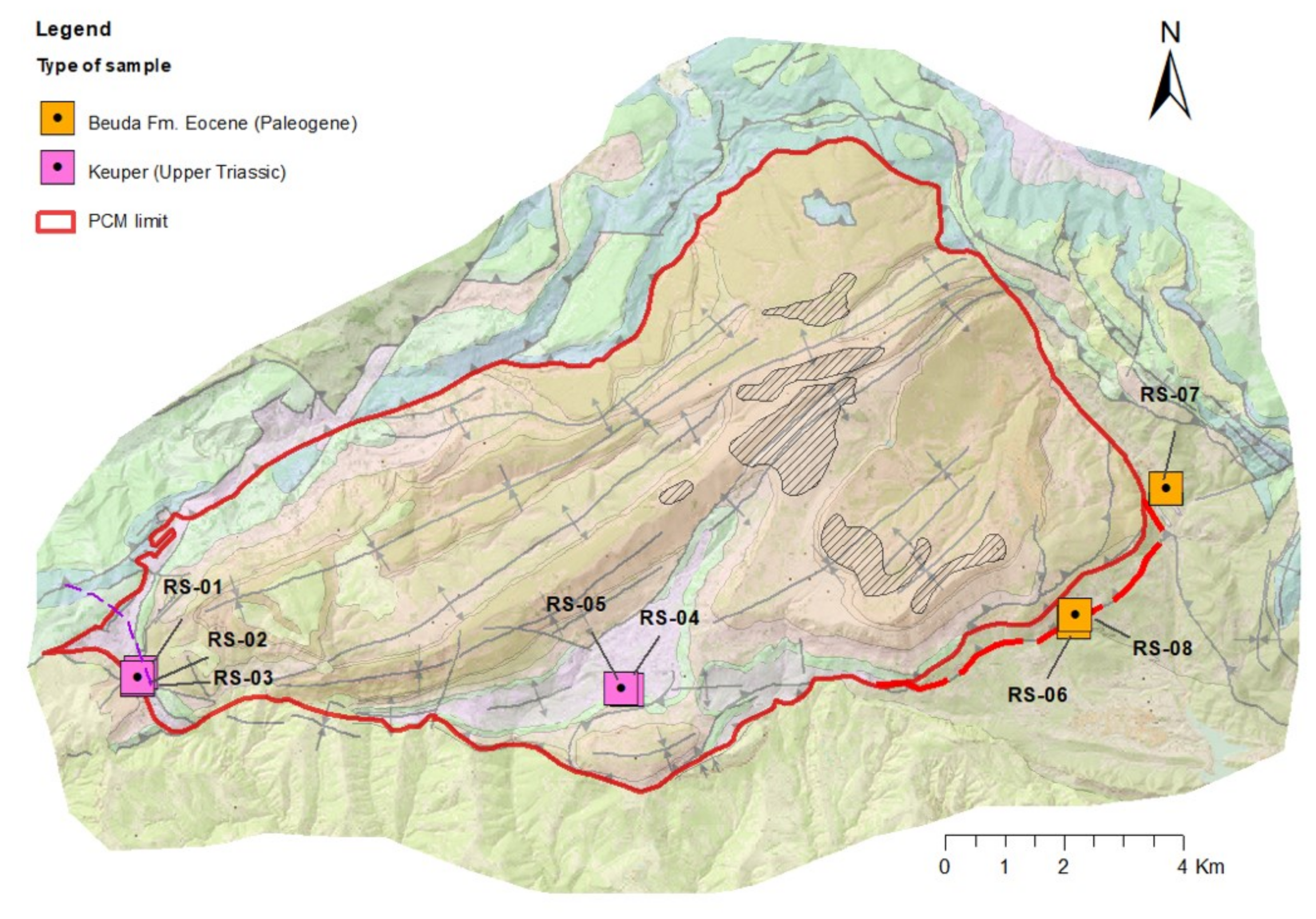
3.2. Application of the Dual-Isotope Approach for δ³⁴S and δ¹⁵N

The existence of NO₃ and SO₄ in GW may pose an environmental risk in many mountains and rural areas with pristine waters. The use of stable isotopes of N and O of dissolved NO₃ and S and O of dissolved SO₄, together with the geochemical data, has proven to be a useful tool to evaluate the origin of solutes [7,20,72,73]. These tools help to improve the knowledge of the hydrogeological system, but also to understand both the natural and anthropogenic geochemical processes driving the GW quality in the aquifer system. In this research, stable isotopes of δ¹⁵N_NO3 and δ¹⁸O_NO3 as well as δ³⁴S_SO4 and δ¹⁸O_SO4 were used to identify NO₃ and SO₄ sources in groundwater using the well-known dual isotope approach [74]. Ranges of NO₃ and SO₄ isotope compositions of the main potential sources were obtained from [73].

3.3. Determination of Proportional Contributions of NO₃ and SO₄ Sources

To estimate the relative contribution of different sources, stable isotope mixing models have become a common tool in environmental studies. Beyond the well-known limitations of the classical mass-balance mixing models—related to the restriction of taking at maximum n + 1 sources for n isotopes [75]—nowadays, the Bayesian isotope mixing models (BMMs) [76,77] are the focus of attention to determine the probable source apportionment. BMMs are traditionally used to identify biogeochemical sources. They allow estimation of the probability distribution for the relative contribution of each source considering the uncertainty associated within the sources themselves and their isotopic compositions. Since a few years ago, these techniques have been used to assess the contribution of NO₃ pollution in general studies [78,79,80,81,82,83,84]. They have also been used specifically in karst studies [85,86], and in very few cases for SO₄ studies [87,88]. Different BMM codes for R and MATLAB have been reported, among them: SIAR, MixSIR, SIMMR, and MixSIAR. In this research, the Stable Isotope Mixing Model (SIMMR) package for R, an updated version of the Bayesian isotope mixing model named as SIAR [76,77], was used to determine the proportional contributions of natural and anthropogenic NO₃ and SO₄ sources into groundwater. The SIAR model (Stable Isotope Analysis in R) is an open-source software package for R. It uses a Markov chain Monte Carlo method to simulate plausible source proportions. The SIAR model is formulated according to Equations (1)–(4):

$$X_{ij}={{\displaystyle \sum }}_{k=1}^K{p}_k·\left(S_{jk}+c_{jk}\right)+{\epsilon }_{ij}$$

(1)

$$S_{jk}~ N\left({\mu }_{jk},{\omega }_{kj}^2\right)$$

(2)

$$c_{jk}~ N\left({\lambda }_{jk},{\tau }_{kj}^2\right)$$

(3)

$${\epsilon }_{ij}~ N\left(0,{\sigma }_j^2\right)$$

(4)

where $X_{ij}$ is the isotope value $j$ of the mixture $i$, in which $i$ = 1, 2, 3,…, N and $j$ = 1, 2, 3,…, J; $S_{jk}$ is the source value $k$ on the isotope $j$ ($k$ = 1, 2, 3,…, K) and is normally distributed with mean ${\mu }_{jk}$ and standard deviation ${\omega }_{kj}^2$; $p_k$ is the proportion of source $k$, which is estimated by the SIAR model; $c_{jk}$ is the fractionation factor for isotope $j$ on source $k$ and is normally distributed with mean ${\lambda }_{jk}$ and standard deviation ${\tau }_{kj}^2$; and finally, ${\epsilon }_{ij}$ is the residual error representing the additional unquantified variation between individual mixtures and is assumed to be normally distributed with mean 0 and standard deviation ${\sigma }_j^2$.

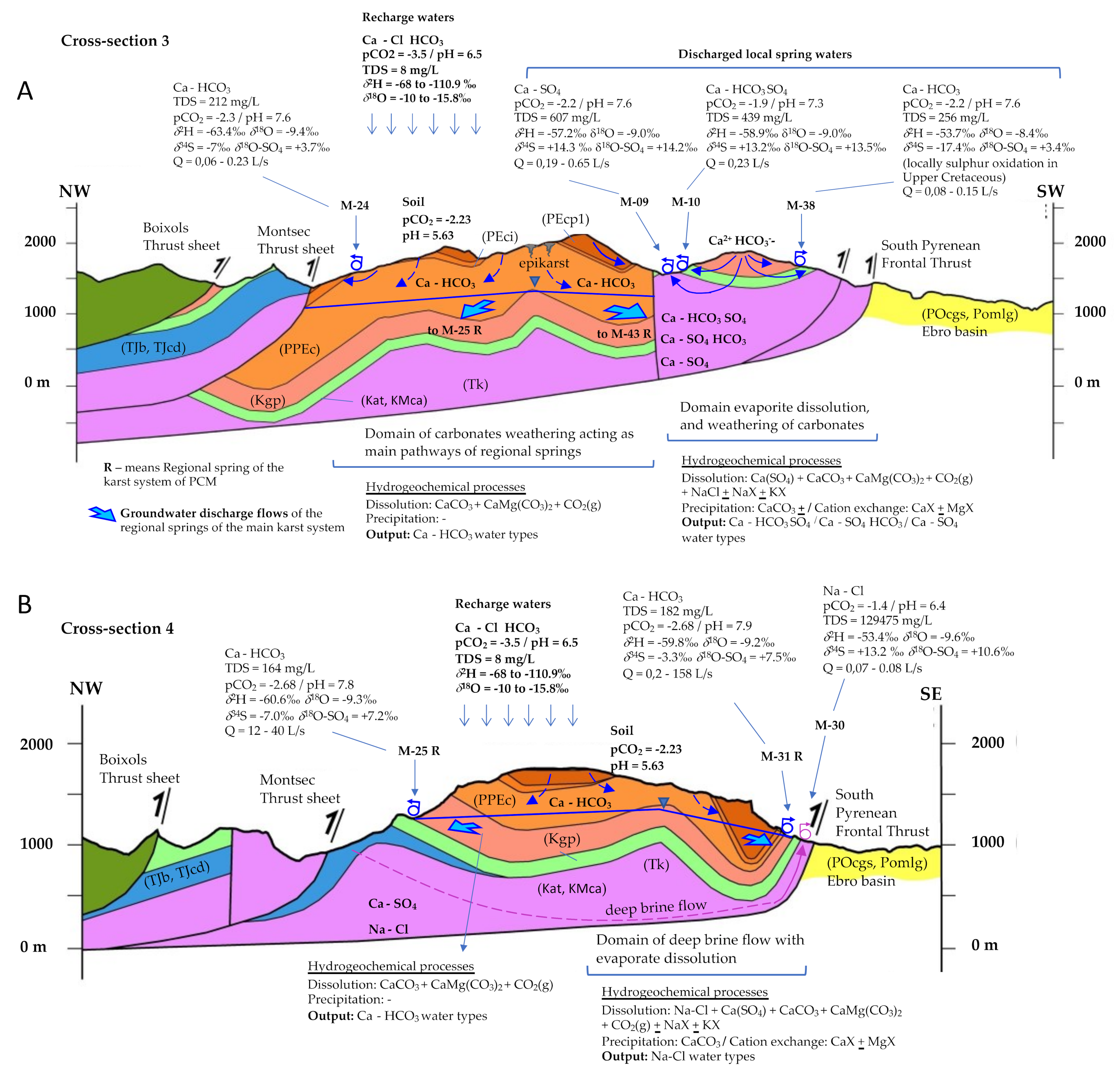
3.4. Delineation of the Main Recharge-Discharge Pathways

The stable isotopes of water δ²H_H20 and δ¹⁸O _H20 values were used by [29] to study the response of the hydrologic system to the seasonal variation of the isotope content in the recharge waters, estimating the Local Meteoric Water Line (LWML) and the local Isotopic Altitudinal Lines (IALs) for δ²H_H20 and δ¹⁸O_H20. In this work, the IAL is used to support the building of the hydrogeochemical conceptual model. To this end, the main Recharge-Discharge Pathways (RDP) of the system are delineated based on (1) the estimated centroid of the recharge zone elevation associated with every spring, and (2) the geological structure of the PCM.

3.5. Inverse Hydrogeochemical Modeling for the Quantification of Chemical Processes

Using the PHREEQC code [70], mass-balance inverse geochemical models are applied to analyze the chemical changes that occur from the recharging areas to the discharge points, and to validate the conceptual hydrogeochemical model of the PCM. Inverse modelling is based on a geochemical mole-balance model, which calculates the transfer of moles of minerals and gases that must enter or leave a solution, while accounting for the differences in an initial and a final water composition along a hypothetic GW flow line. In this work, the study is focused on 14 springs that are considered representative of the main Recharge-Discharge Pathways (RDP) of the system, which were previously defined based on the recharge elevations inferred by means of the IALs. The differences in hydrogeochemical composition between the springs are assumed to be due exclusively to reactions between GW and the minerals within the PCM. The selection of the solid phase reactants is based on the geological knowledge of the main lithologies, which comprise calcite, dolomite, gypsum, and halite. In addition, soil gas CO₂ is also considered. The existence of marl and clay materials in the limits of the PCM, as in the Cretaceous and Triassic materials, suggests that ionic exchange-like processes between cations Ca, Mg, Na, and K and an exchanger X might occur. As all water samples are undersaturated according to the calculated saturation index, the inverse modeling was constrained so that dolomite, gypsum, and halite only dissolve whereas calcite is allowed to both dissolve and precipitate. In summary, the expected reactions responsible for the groundwater composition can be defined as:

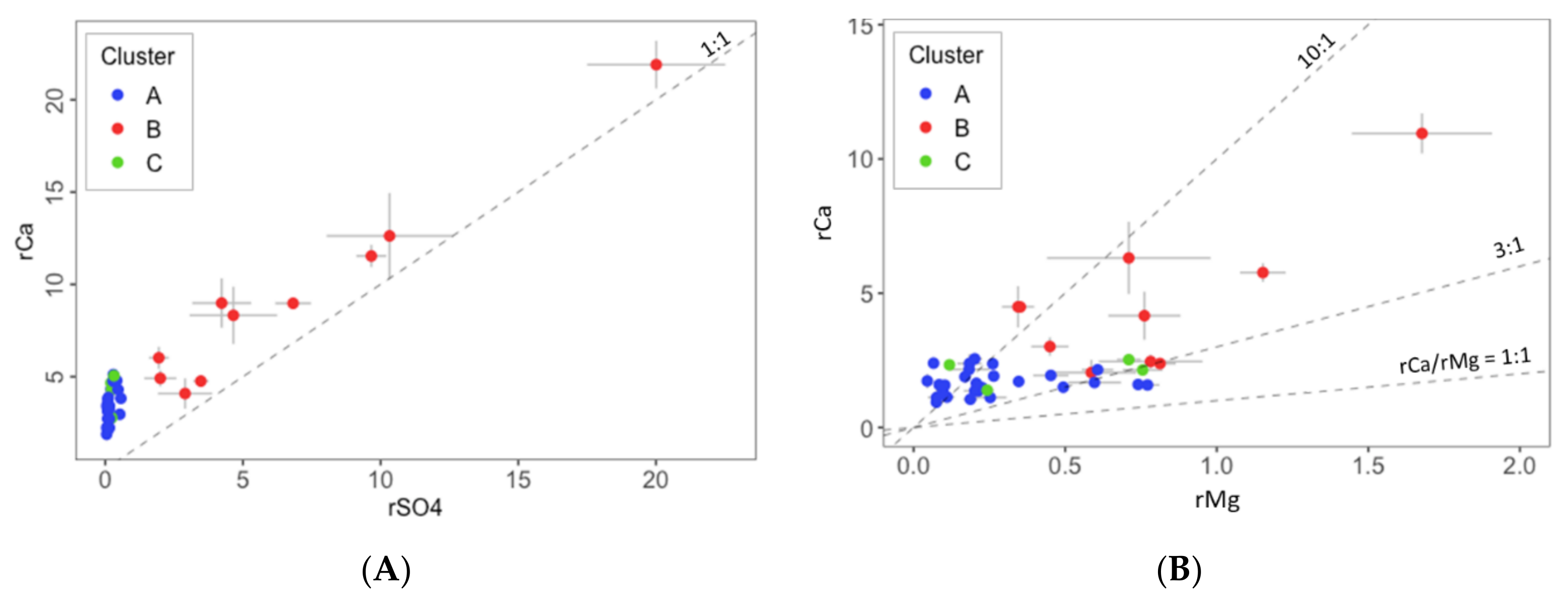
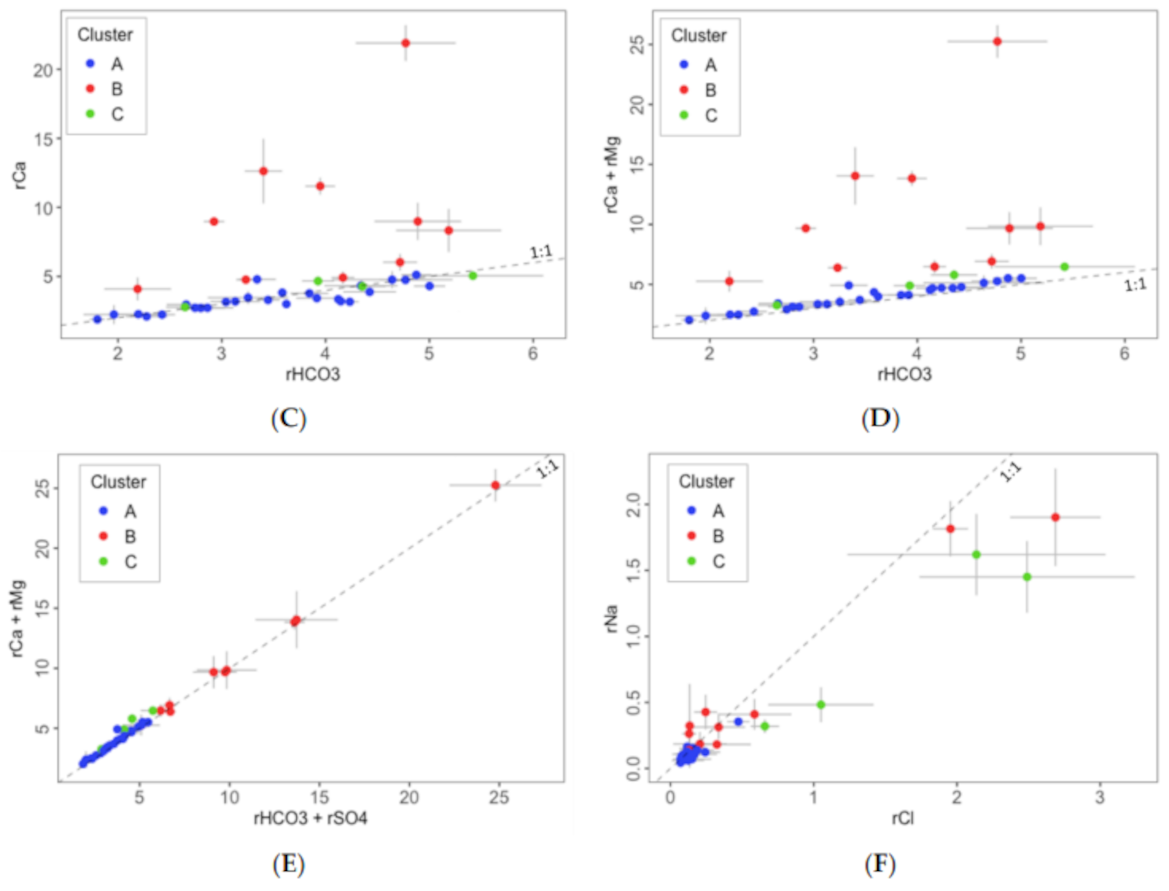
• Dissolution of carbonate minerals, such as calcite and dolomite, and precipitation of calcite according to Equations (5) and (6) [89]. Equation (7) is obtained as the sum of Equations (5) and (6), and it shows that the molar ratio Ca²⁺/Mg²⁺ is 3:1:

  $$2{\mathrm{CaCO}}_3+2{\mathrm{CO}}_2\left(\mathrm{g}\right)+2{\mathrm{H}}_2\mathrm{O}\leftrightarrow 2{\mathrm{Ca}}^{2+}+4{\mathrm{HCO}}_3^{-}$$

  (5)

  $$2\mathrm{CaMg}{({\mathrm{CO}}_3)}_2+4{\mathrm{CO}}_2\left(\mathrm{g}\right)+4{\mathrm{H}}_2{\mathrm{O}\leftrightarrow \mathrm{Ca}}^{2+}+{\mathrm{Mg}}^{2+}+8{\mathrm{HCO}}_3^{-}$$

  (6)

  $$2{\mathrm{CaCO}}_3+2\mathrm{CaMg}{({\mathrm{CO}}_3)}_2+6{\mathrm{CO}}_2\left(\mathrm{g}\right)+6{\mathrm{H}}_2\mathrm{O}\leftrightarrow 3{\mathrm{Ca}}^{2+}+{\mathrm{Mg}}^{2+}+12{\mathrm{HCO}}_3^{-}$$

  (7)
• Dissolution of evaporite minerals, such as gypsum and halite, according to Equations (8) and (9):

  $${\mathrm{CaSO}}_4·2{\mathrm{H}}_2\mathrm{O}\leftrightarrow {\mathrm{Ca}}^{2+}+{\mathrm{SO}}_4^{2-}+2{\mathrm{H}}_2\mathrm{O}$$

  (8)

  $$\mathrm{NaCl}\leftrightarrow {\mathrm{Na}}^{+}+{\mathrm{Cl}}^{-}$$

  (9)
• Dedolomitization processes according to Equation (10) [71], which causes an increment of Ca²⁺ due to gypsum dissolution (as indicated in Equation (8)) and precipitation of calcite:

  $$\mathrm{CaMg}{({\mathrm{CO}}_3)}_2+{\mathrm{CaSO}}_4·2{\mathrm{H}}_2\mathrm{O}\leftrightarrow 2{\mathrm{CaCO}}_3+{\mathrm{Mg}}^{2+}+{\mathrm{SO}}_4^{2-}+2{\mathrm{H}}_2\mathrm{O}$$

  (10)
• Ion exchange reactions due to weathering reactions in marls, shales, and clays associated with Triassic and Cretaceous layers, according to the following Equations (11)–(14):

  $$2\mathrm{NaX}+{\mathrm{Ca}}^{2+}\leftrightarrow 2{\mathrm{Na}}^{+}+{\mathrm{CaX}}_2$$

  (11)

  $$2\mathrm{NaX}+{\mathrm{Mg}}^{2+}\leftrightarrow 2{\mathrm{Na}}^{+}+{\mathrm{MgX}}_2$$

  (12)

  $$2\mathrm{KX}+{\mathrm{Ca}}^{2+}\leftrightarrow 2{\mathrm{K}}^{+}+{\mathrm{CaX}}_2$$

  (13)

  $$2\mathrm{KX}+{\mathrm{Mg}}^{2+}\leftrightarrow 2{\mathrm{K}}^{+}+{\mathrm{MgX}}_2$$

  (14)

Silicate minerals in the aquifer were generated in the marine environment in which the carbonates were deposited, and this affects the sorbed cation composition. Dispersed silicates in the carbonate rock matrix may progressively contribute Na⁺ as carbonates are dissolved, as well as a fraction of the K⁺, at the time that HCO₃ increases. This is a minor process. Marl and clay layers may contain evaporitic minerals that slowly diffuse out, contributing Cl⁻, SO₄²⁻, and cations that correspond approximately to halite and gypsum dissolution, although with a modified cation composition. All these processes can be assumed steady in a hydrogeological system under natural conditions, so cation exchange is minor and not significant. However, the silicate weathering and porewater diffusion in clays produce similar results as cation exchange, and therefore they are considered as such for general treatment and called cation exchange-like process.

There are no data on soil CO₂ partial pressure and therefore this value and the carbon isotopic composition must be assumed. Then, the CO₂ dissolved in the meteoric water recharging the aquifer is assumed to be (1) in equilibrium with atmospheric CO₂ partial pressure for elevations above 1900 m a.s.l. and equal to log(PCO₂) = −3.2 (no vegetation), and (2) equilibrated with the soil CO₂ for elevations below 1900 m a.s.l., with the CO₂ content estimated by the following equation [71] to consider the existence of decaying vegetation and root respiration:

$$\log \left({\mathrm{PCO}}_2\right)=-3.47+2.09(1-{\mathrm{e}}^{-0.00172·\mathrm{ETP}})$$

(15)

where PCO₂ corresponds to the mean growing-season soil CO₂ partial pressure and ETP is the mean potential evapotranspiration. The mean ETP in the PCM is 525 mm/year [90] and the obtained log(PCO₂) is −2.23.

Considering the geological structure of the PCM along with the estimated average recharge altitude associated to every sampled spring, a total of 14 representative Recharge-Discharge Pathways, named as RDPs 1 to 14 (Figure 3), were considered for inverse hydrochemical modeling with PHREEQC.

Every RDP tries to recreate the GW flow line integrating all the processes driving the hydrochemical composition of the corresponding spring discharge, from which the RDP adopts the cluster type. Therefore, the RDPs are classified in clusters as:

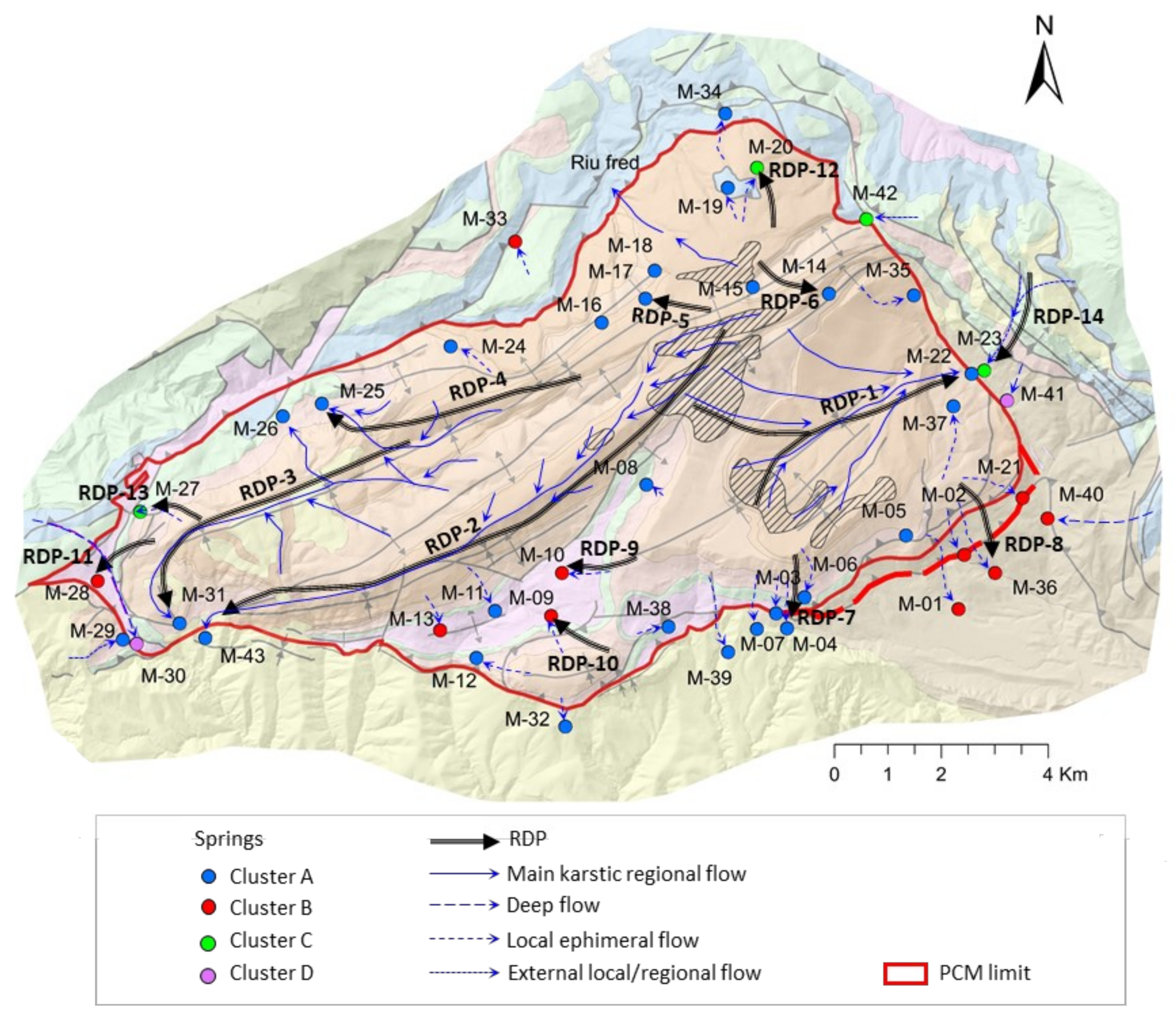
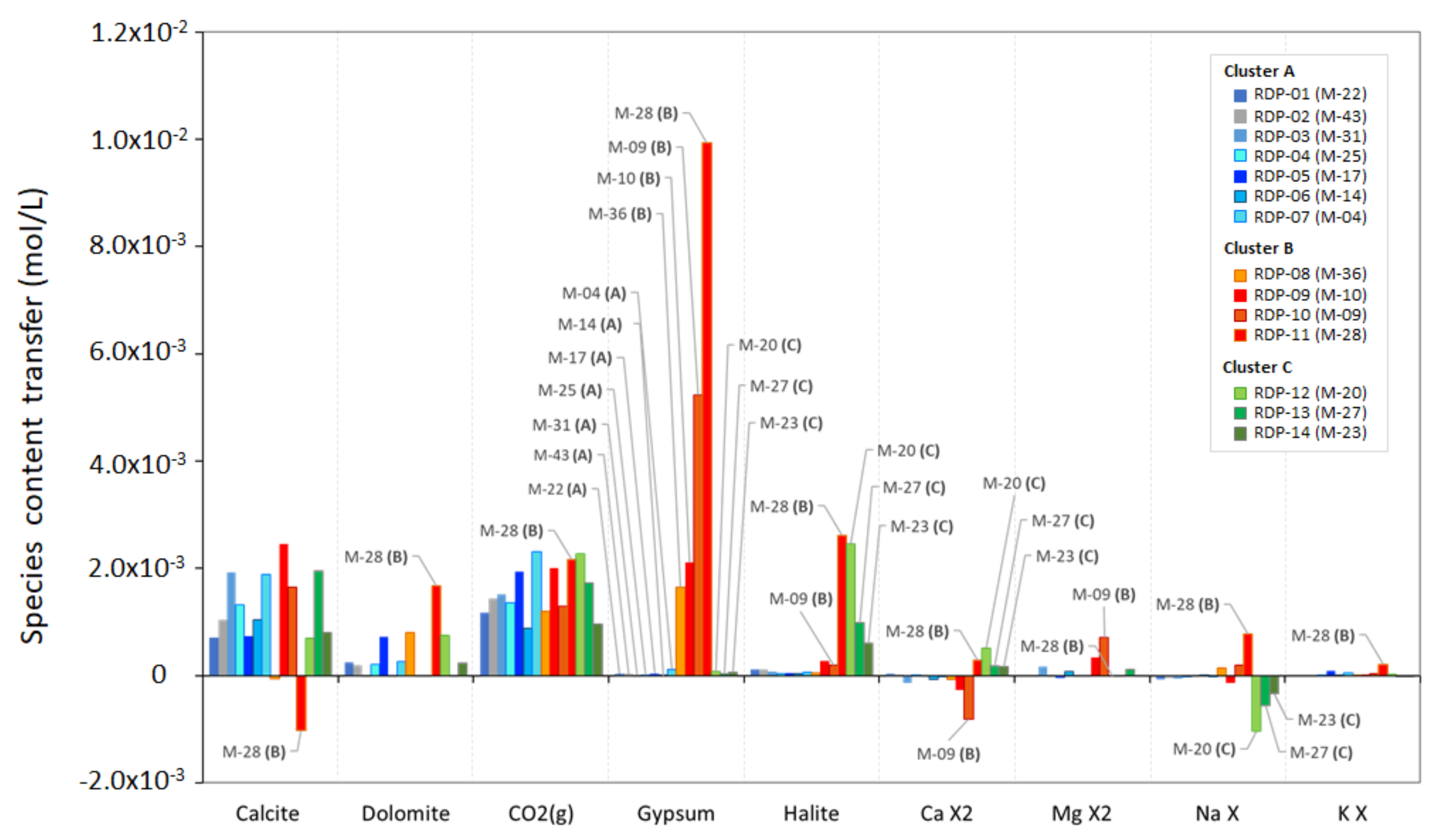
• RDP-Cluster A: RDP-1 to RDP-4 correspond to the four regionals springs (M-22, M-43, M-31, and M-25). RDP-05 is related to the springs located in the upper part of the PCM (M-16, M-17, M-18, and M-19) that discharge to the north and are oversaturated with respect to dolomite. On the contrary, RDP-06 refers to the other two springs located in the upper part of the PCM (M-14 and M-15) draining to the south, which are under-saturated with respect to dolomite. RDP-07 is related to the five local springs M-06, M-03, M-04, M-07, and M-39 of Cluster A that drain the southern part of the PCM through fractures that affect the PPEc unit or contact the underlying Kgp unit.
• RDP-Cluster B: RDP-08 represents the flow line associated with the four springs M-01, M-02, M-36, and M-21 that drain through the southeast part of the PCM while being affected by the presence of the Eocene-Oligocene Beuda’s gypsum Formation. RDP-09 and RDP-10 are associated with the local springs M-10 and M-09, respectively. According to the recharge elevation zone associated with these springs, the meteoric water enters the system through the Kgp unit. Then GW flows downstream through the Kat and KMca units and finally discharges through the Tk unit. RDP-11 is associated with M-28 spring, whose recharge zone is in the PPEc unit. Then, GW flows through the Cretaceous and discharges through the Tk unit.
• RDP-Cluster C: RDP-12 and RDP-13 correspond to local RDPs running through the Tk unit that contains halite. These two RDPs are located at the NW and W of the PCM, respectively. Finally, RDP-14 is a flow path out of the PCM boundaries and associated with spring M-23, a spring with a water-type like that of the neighboring spring M-22 (Figure 2A).

4. Results and Discussion

The hydrochemical and isotope data of GW corresponding to the different sampling campaigns conducted in this work are reported in Table A1, Table A2, Table A3,

Table A4. Chemical characteristics of major constituents for the 10 snow samples (7 natural and 3 artificial) and 2 water ponds. (samples type T-1 correspond to artificial snow (snow gun); T-2 natural snow (inside sky trail); T-3 natural snow (outside sky trail); and T-4 water ponds for artificial snow production.

ID	Date	Water Type	Sample Type	EC [μS/cm]	TDS [ppm]	pH	T [ºC]	Ca [ppm]	Mg [ppm]	Na [ppm]	K [ppm]	HCO3 [ppm]	CO3 [ppm]	Cl [ppm]	NO3 [ppm]	SO4 [ppm]	δ2HH20 (‰)	δ18OH20 (‰)
M-09as	09/12/13	Ca-HCO3 Cl	T-1	49	24	10.3	-	5.6	0.5	1.3	1.2	11.6	2.9	4.9	1.6	1.6	−41.4	−5.1
M-120	07/12/14	Ca-HCO3	T-1	142	71	10.0	-	18.0	4.0	6.3	1.2	55.0	12.0	9.3	1.3	5.0	−45.0	−5.9
M-100	07/12/14	Ca-HCO3	T-1	51	26	9.6	-	8.9	1.0	1.2	0.2	24.0	<2.4	2.5	<1	1.1	−51.6	−7.5
M-08ps	09/12/13	Ca Na-Cl	T-2	25	13	7.0	-	<2	<0.4	1.4	1.3	3.0	<2.4	4.0	0.2	<0.7	−110.9	−15.8
Ms-11	09/03/14	Ca-Cl HCO3	T-2	21	11	6.7	-	<2	<0.4	1.0	0.9	3.5	<2.4	<2.5	2.9	<0.7	−70.0	−10.2
Ms-09	09/03/14	Ca-Cl HCO3	T-2	16	8	6.2	-	<2	<0.4	1.0	0.4	2.7	<2.4	<2.5	2.3	<0.7	−88.3	−12.4
Ms-08	09/03/14	Ca-Cl	T-2	21	10	5.6	-	<2	<0.4	1.0	0.7	1.2	<2.4	<2.5	3.5	<0.7	−101.0	−14.1
Ms-12	09/03/14	Ca-Cl HCO3	T-2	13	6	5.7	-	<2	<0.4	1.0	0.4	2.5	<2.4	<2.5	1.9	<0.7	−68.7	−10.3
M-07ps	07/12/13	Ca-Cl HCO3	T-3	5	2	6.7	-	<2	<0.4	1.0	0.3	2.7	<2.4	2.5	0.3	<0.7	−105.8	−14.8
M-10ps	12/01/14	Ca-Cl HCO3	T-3	20	9	5.5	-	<2	<0.4	1.0	0.2	3.7	<2.4	4.2	<1	1.4	−88.1	−11.7
M-80	23710/14	Ca-HCO3	T-4	142	71	8.3	10.6	28.0	1.8	1.6	0.7	83.0	<2.4	4.2	<1	3.3	−50.7	−7.0
M-70	23/10/14	Ca-HCO3	T-4	177	88	8.2	10.2	27.0	3.5	4.8	1.0	74.0	<2.4	19.9	1.7	5.3	−43.6	−6.0

, Table A5,

Table A6. Average values for δ³⁴S_SO4 and δ¹⁸O_SO4 of samples available of all springs and the corresponding average SO₄ concentration.

Spring	Cluster	Num. Samples	GU (BG50M)	SO4 [ppm]	Water Type	δ34SSO4 (‰)	δ18OSO4 (‰)
M-03	A	2	PEalb	4.44	Ca-HCO3	+7.6	+5.8
M-04	A	21	POcgs	16.29	Ca-HCO3	+3.9	+8.1
M-05	A	1	Qpe	3.39	Ca-HCO3	+6.4	+9.7
M-06	A	2	Kgp	9.82	Ca-HCO3	+0.4	+8.0
M-07	A	3	POcgs	14.14	Ca-HCO3	+8.3	+10.9
M-08	A	2	Kgp	8.72	Ca-HCO3	+11.6	+13.7
M-11	A	3	KMca	25.13	Ca-HCO3	+10.8	+12.5
M-12	A	1	Kgp	4.03	Ca-HCO3	+4.7	+6.3
M-19	A	2	TJcd	4.52	Ca-HCO3	+6.0	+5.5
M-22	A	21	Qvl	7.07	Ca-HCO3	−3.3	+7.6
M-24	A	2	PPEc	5.44	Ca-HCO3	−7.0	+3.7
M-25	A	20	Kgp	Kgp	Ca-HCO3	−7.0	+7.2
M-26	A	1	KMca	4.94	Ca-HCO3	+3.1	+10.5
M-29	A	3	Qpe	28.42	Ca-HCO3	+10.9	+11.1
M-31	A	19	PPEc	4.45	Ca-HCO3	−3.3	+7.5
M-32	A	2	POmlg	19.72	Ca-HCO3	+3.2	+8.2
M-34	A	3	TJb	6.93	Ca-HCO3	+6.1	+8.1
M-35	A	1	PEcp1	4.49	Ca-HCO3	−0.6	+13.7
M-37	A	2	Qvl	3.89	Ca-HCO3	+3.5	+7.2
M-38	A	3	Kat	21.52	Ca-HCO3	−17.5	+3.4
M-39	A	2	POmlg	14.69	Ca-HCO3	+7.8	+9.7
M-43	A	21	POcgs	6.66	Ca-HCO3	−4.5	+8.2
M-01	B	2	PEm1	106.52	Ca-HCO3	+12.8	+10.1
M-02	B	4	PEmb	139.26	Ca-SO4 HCO3	+13.2	+10.2
M-09	B	4	Tk	495.92	Ca-SO4	+14.4	+14.2
M-10	B	4	Tk	203.08	Ca-SO4 HCO3	+13.2	+13.5
M-13	B	4	Tm	96.03	Ca-HCO3 SO4	+13.2	+13.3
M-21	B	4	Qcoo	327.72	Ca-SO4	+20.4	+13.2
M-28	B	4	Tk	961.12	Ca-SO4	+13.8	+14.1
M-33	B	4	Tk	223.46	Ca-SO4 HCO3	+9.1	+10.6
M-36	B	4	PEmb	166.82	Ca-SO4 HCO3	+8.5	+8.7
M-40	B	4	Tk	464.13	Ca-SO4	+20.0	+12.7
M-20	C	22	PEcp2	10.8	Ca-HCO3 Cl	+10.2	+9.1
M-23	C	2	Qt0	12.2	Ca-HCO3	+11.2	+11.1
M-27	C	2	KMca	9.7	Ca-HCO3	+7.7	+8.8
M-42	C	3	KMca	14.9	Ca-HCO3	−5.1	+3.5
M-30	D	4	Tk	8138.20	Na-Cl	+13.2	+10.6
M-41	D	4	Tk	1264.67	Na-Cl	+18.6	+12.4

, Table A7 and

Table A8. Average values for δ¹⁵N_NO3 and δ¹⁸O_NO3, of samples available of all springs and the corresponding average NO₃ concentration.

Spring	Clust	Num. Samples	GU (BG50M)	NO3 [ppm]	Water Type	δ15NNO3 (‰)	δ18ONO3 (‰)
M-04	A	11	POcgs	4.15	Ca-HCO3	4.3	3.7
M-11	A	2	KMca	10.76	Ca-HCO3	0.5	0.0
M-14	A	1	PPEc	11.69	Ca-HCO3	−0.1	0.7
M-19	A	3	TJcd	6.06	Ca-HCO3	−0.9	1.0
M-22	A	4	Qvl	5.62	Ca-HCO3	4.8	4.5
M-26	A	1	KMca	2.54	Ca-HCO3	−0.1	0.0
M-29	A	3	Qpe	8.78	Ca-HCO3	7.0	1.5
M-31	A	4	PPEc	3.73	Ca-HCO3	4.3	4.8
M-32	A	3	POmlg	57.27	Ca-HCO3	0.3	1.4
M-43	A	2	POcgs	3.64	Ca-HCO3	4.1	3.9
M-01	B	2	PEm1	6.16	Ca-HCO3	3.1	3.0
M-02	B	2	PEmb	4.58	Ca-SO4 HCO3	−0.1	1.4
M-09	B	2	Tk	4.90	Ca-SO4	1.9	1.5
M-10	B	3	Tk	18.14	Ca-SO4 HCO3	1.2	2.6
M-28	B	3	Tk	38.60	Ca-SO4	10.7	3.7
M-20	C	21	PEcp2	11.3	Ca-HCO3 Cl	3.7	0.7
M-23	C	2	Qt0	4.4	Ca-HCO3	7.4	8.0
M-27	C	1	KMca	2.1	Ca-HCO3	1.6	3.1
M-30	D	1	Tk	4.49	Na-Cl	9.6	6.2
M-41	D	1	Tk	6.75	Na-Cl	7.7	1.6

, Appendix A.

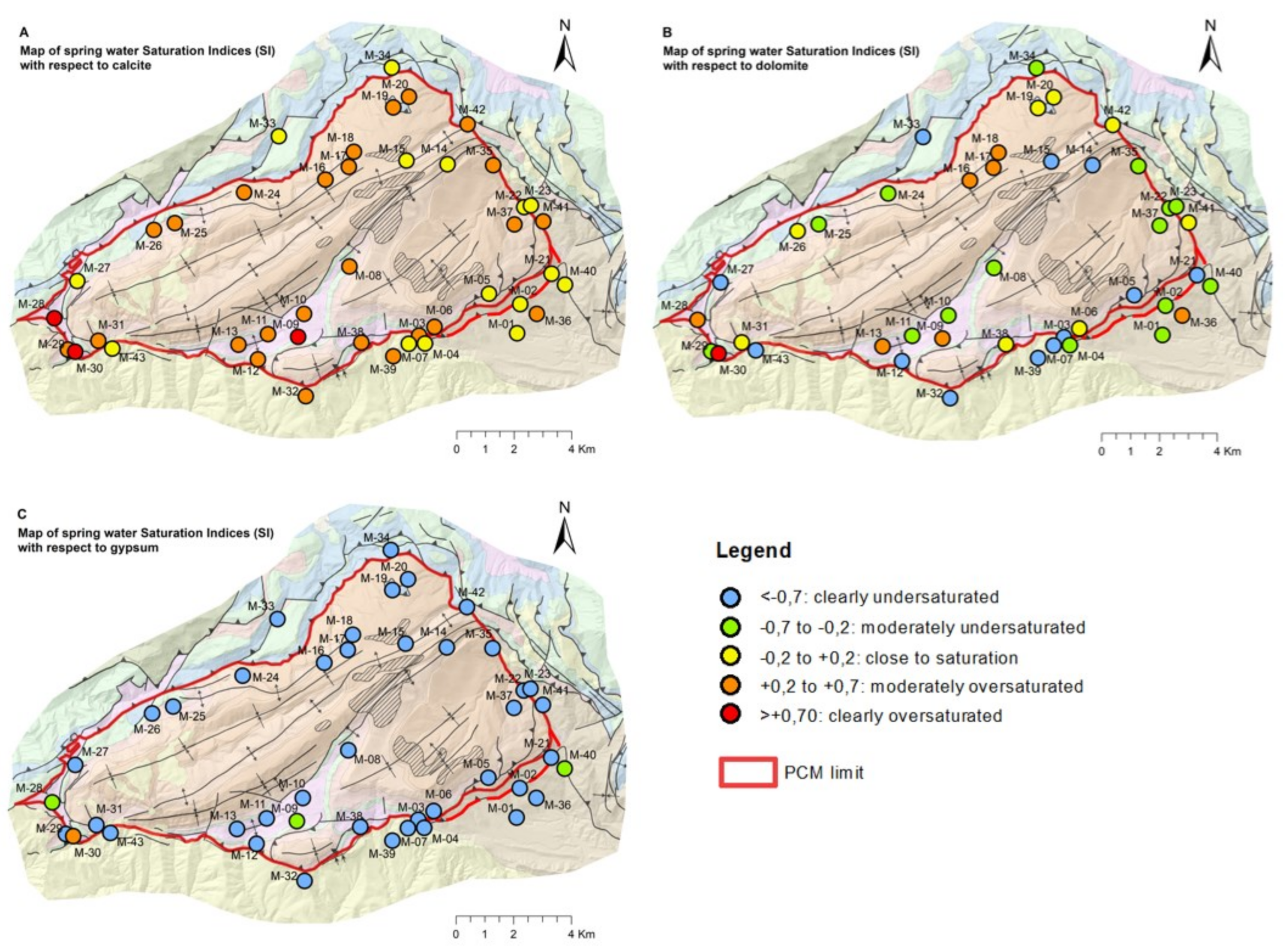
4.1. Saturation Indexes

The saturation indexes (SIs) were calculated using PHREEQC^® [70]. The SI relative to calcite for all the dataset ranges from 0 to 0.82, indicating calcite saturation to oversaturation throughout the PCM (Figure 4A). The SI relative to dolomite ranges from −1.32 to 0.61, except for a 2.3 value corresponding to the deep flow brine spring M-30 (Figure 4B). The SI relative to gypsum ranges from −3.26 to 0.27 (the highest value in M-30), between under-saturated to almost equilibrium conditions within the Triassic (Keuper) window and the Tertiary window (Eocene-Oligocene Beuda’s gypsum Formation, which is pinched out within the South Pyrenees thrust fault in the front SE of the PCM), affecting the springs M-21, M-40, M-01, M-02, and M-36 (Figure 4C).

Figure A4 shows the relationship between SI relative to calcite, dolomite, gypsum, and halite with respect to TDS [mg/L], besides SI of gypsum with respect to SI of halite, and SI of calcite with respect to SI of gypsum. In all cases, it is possible to observe a clear separation between all the clusters A, B, C, and D. In addition, a trend of increasing TDS can be observed from clusters A, C towards cluster B, and later to the extreme D.

In general, the springs of cluster A have lower TDS than those of cluster B. Figure 5A shows that despite all the samples being in equilibrium or slightly supersaturated with respect to calcite, cluster A shows much less TDS content than cluster B. Additionally, Figure 5B indicates that most of the samples are subsaturated relative to dolomite, except in four samples from cluster A (springs M-16, M-17, M-18, and M-19 located in the northern part of the PCM that discharge the PPEc unit in contact with the PEci unit), four samples from cluster B (M-28, M-36, M-09, M-13), and one sample from cluster C (M-20) that is close to the equilibrium relative to dolomite. Figure 5C shows how all the springs but one (M-30 from cluster D) are under-saturated with respect to gypsum. Moreover, here the separation between clusters A and C with respect to B and D can be clearly observed, indicating that the samples of cluster B are influenced by Triassic (Keuper) and Tertiary (Beuda Formation) formations that contain gypsum. Furthermore, the clusters’ separation is even clearer when looking at the relationship between SI relative to halite and TDS (Figure 5D), SI of gypsum, and SI of halite (Figure 5E), and less evident for SI of calcite and SI gypsum (Figure 5F).

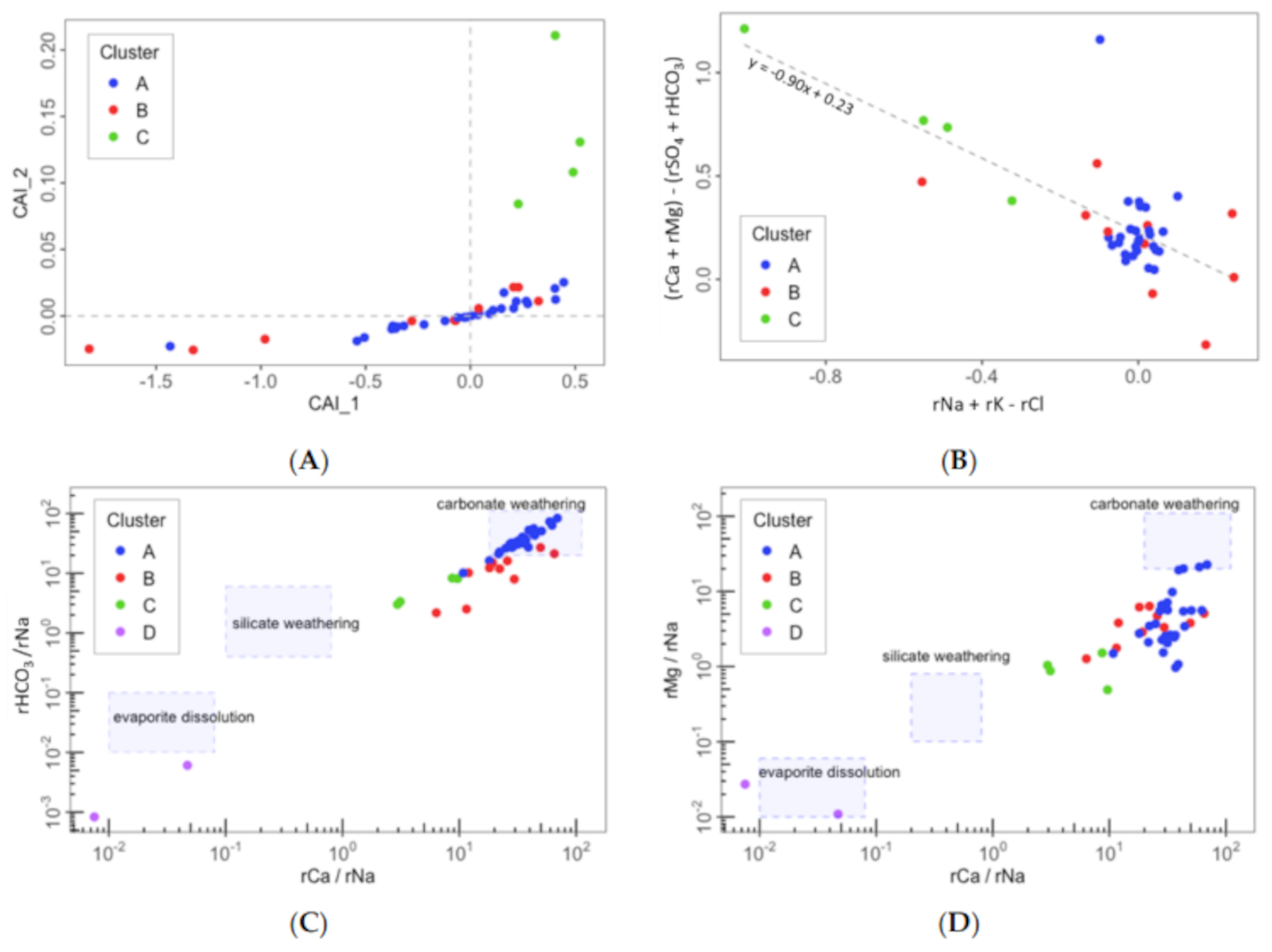
4.2. Identification of Hydrogeochemical Processes Explaining the Spring Clusters

To determine the main rock–water interactions within the PCM system driving the hydrogeochemical composition of GW, it is necessary to focus on the relationships between major cations and anions. This will help to decipher the main hydrogeochemical processes conditioning the cluster definition presented by [59]. The data presented in this analysis for every spring corresponds to average content values for the monitored period September 2013–October 2015 (Table A2 Appendix A).

The relationship between Ca and SO₄ is depicted in Figure 5A. The samples of cluster B follow the line of slope 1:1, thus indicating most probably the dissolution of gypsum as the origin of sulfate in cluster B, while cluster A and C are not clearly related with this process. This suggests that calcite and dolomite are not the primary sources of Ca for cluster B, but they might be for cluster A and C.

The relative contribution of calcite and dolomite in the carbonate weathering processes can be approached by looking at the molar ratio rCa/rMg (r = concentration in meq/L) (Figure 5B). A molar ratio of 1 (1:1 slope line) indicates pure dolomite contribution (Equation (6), ratio values between 1 and 3 indicate a dominance of dolomite dissolution with some calcite contribution, rCa/rMg = 3 indicates dissolution of both calcite and dolomite according to Equation (7)). Larger ratio values mean a predominance of calcite dissolution plus certain dolomite contribution, and finally, rCa/rMg = 10 represents a total contribution of calcite, beyond the evident contribution of sulphate dissolution in cluster B, as indicated in Figure 5A. As can be shown, all the GW samples have rCa/rMg > 1. Almost 50% of the molar ratio values range between 3 and 10, and 16% between 1 and 3. Cluster A shows 12 springs with rCa/rMg >10, 11 springs with 3 < rCa/rMg < 10, and four springs with rCa/rMg < 3. The four springs of this latter case (M-16, M-17, M-18, and M-19) also show saturation indices (SI) relative to dolomite > 1. Dolomite is present in the recharge area within the PPEc unit. Cluster B contains two springs (M-10 and M-21) with rCa/rMg > 10, seven springs with 3 < rCa/rMg < 10, and one spring (M-36) with rCa/rMg < 3. Cluster C shows one spring (M-27) with rCa/rMg >10, two springs (M-23 and M-42) with 3 < rCa/rMg < 10, and one spring with rCa/rMg < 3. The two springs of cluster D show rCa/rMg values equal to 0.18 (M-30) and 4.32 (M-41). These results suggest that, except for the four cited samples from cluster A that drain the upper part of the PCM, where the materials associated with the PPEc unit are richer in dolomite, the contribution of dolomite increases as the discharge altitude decreases.

The influence of calcite dissolution on cluster A can be observed looking at the ratio rCa/rHCO₃ in Figure 5C. Here, the samples of the cluster A plot align along the line of slope 1:1, representing the stoichiometric ratio of calcite dissolution. To evaluate the influences of the combined dissolution of calcite and dolomite on karst groundwater chemistry, Figure 5D shows the ratio between rCa + rMg with respect to rHCO₃. The plot shows that one part of the data for cluster A fits the 3: 1 slope line, suggesting that both dissolution of calcite and dolomite contributes to defining groundwater chemistry, whereas the remainder seems to be concentrated at the base of the 10:1 slope, indicating exclusive contribution from calcite. In the case of cluster C, the four springs plot displaced above while maintaining the slope 1:1, which might be related to ion exchange-like processes adding Ca into dissolution according to Equation (11). The samples of cluster B are clearly scattered relative to the 1:1 slope line, thus confirming that they have other Ca sources than calcite and/or dolomite dissolution.

To confirm that dissolution of carbonates (calcite and dolomite) and evaporites (gypsum and halite) are the dominant processes affecting the hydrochemical features of the different clusters, and that ion exchange is a minor process driving the hydrogeological composition of GW, the relationship between (rCa + rMg) and (rHCO₃ + rSO₄) is presented in Figure 5E. Most of the springs match the line 1:1 with just very small shifts for clusters B and C, thus suggesting the existence of a very small ion exchange-like process adding Ca and/or Mg into dissolution (Equations (11) and (12)). Figure 5F shows the scatterplot of rNa content versus rCl. In general, the gravity center of all the clusters is below the line of the 1:1 slope, reflecting a chloride excess that principally comes from the atmospheric chloride deposition, although a minor part, especially in the case of samples from cluster B and C, might be attributed to silicate weathering and ion exchange-like reactions in marls, shales, and clays associated with the Triassic and Cretaceous layers through which the groundwater of these springs interacts.

In this regard, and to get more information about the possible contribution of such an exchange-like process, Schoeller (1965) [91] propose using the chloro-alkaline indices indexes, CAI_1 and CAI_2, of common use in hydrogeochemical studies, which are defined as:

$$\mathrm{CAI}\_1=\left(\mathrm{rCl}-\left(\mathrm{rNa}+\mathrm{rK}\right)\right)/\mathrm{rCl}$$

(16)

$$\mathrm{CAI}\_2=\left(\mathrm{rCl}-\left(\mathrm{rNa}+\mathrm{rK}\right)\right)/\left({\mathrm{rHCO}}_3+{\mathrm{rSO}}_4+{\mathrm{rCO}}_3+{\mathrm{rNO}}_3\right)$$

(17)

Values > 0 of both indexes indicate ion exchange and ion exchange-like processes in which dissolved Na and/or K are retained while Ca and/or Mg are released, or Ca-rich brines are incorporated. Values < 0 point to a reverse ion exchange prevalent process [91] or weathering of alkaline ion-rich silicates. In this line, most of the samples do not show a clear sensitivity of CAI_2 with respect to CAI_1 (Figure 6A). Nevertheless, the samples of cluster C are clearly located in the first quadrant where both CAI_1 and CAI_2 are >0.

Figure 6A shows the plot of (rCa + rMg) − (rSO₄ + rHCO₃) versus (rNa + rK − rCl). The dependent variable represents the increment of Ca and Mg that is attributed to processes that exclude weathering by carbonates and evaporites (dissolution of calcite, dolomite, and gypsum) while the independent variable gives information of the increment of Na generated by processes other than halite dissolution. A linear relation between these two variables with a slope equal to −1 indicates the significance of ion exchange-like processes as an important factor controlling the groundwater chemistry and its evolution. In the case of the samples of the PCM, the slope of the regression line between (rCa + rMg) − (rSO₄ + rHCO₃) and (rNa + rK − rCl) is −0.90 (Figure 6B). Such a relationship is basically conditioned by the samples of cluster B and C, which would suggest that there may indeed be ion exchange-like processes between the monovalent ions Na and K, and the bivalent Ca and Mg. Moreover, values of (rCa + rMg) − (rSO₄ + rHCO₃) > 0 indicate adsorption of Na and release of Ca [92].

The relationship between both HCO₃/rNa and rMg/rNa vs. rCa/rNa, in Figure 6C,D, respectively, can be used to check the main geochemical process in the system [15,93,94,95]. In these figures, it can be shown how the origin of HCO₃ for the samples of cluster A is carbonate dissolution. Cluster C and some samples of Cluster B tend to the silicate weathering zone, which also would be related to sodium-calcium ion exchange-like in the weathering of shales. Besides, the two samples of cluster D, corresponding to the deep flow brines, fit in the evaporite window domain.

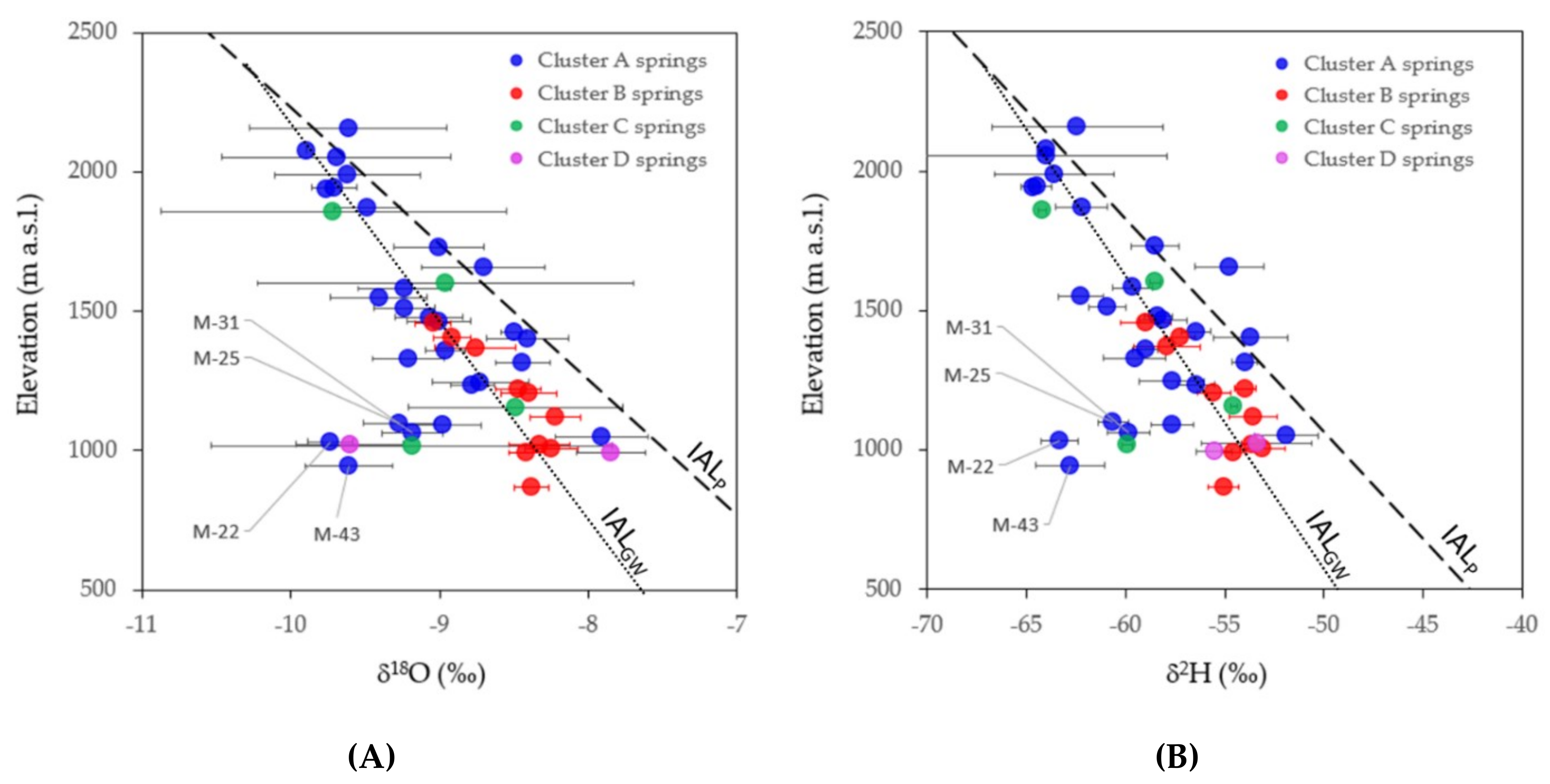
4.3. Aquifer Recharge Altitude Based on δ²H and δ¹⁸O in Precipitation and GW

The estimation of the recharge elevation associated with the springs sampled during this study is conducted by projecting the mean isotopic content of δ²H and δ¹⁸O associated with every spring discharge to the corresponding IAL obtained by [33], which are shown in Figure 7.

Table 1. Recharge elevation associated with GW clusters in the PCM.

	Recharge Elevation (m a.s.l.)			${\nabla }_{\mathbf{z}}{\mathit{\delta }}_{GW} \mathbf{\left(}‰/\mathbf{km}\mathbf{\right)}$
	Average	Min	Max	δ18O	δ2H
Cluster A	1823	1259	2228	−1.5	−9.8
Cluster B	1541	1409	1758	−1.5	−9.7
Cluster C	1776	1557	2010	−1.2	−8.0
Cluster D	1193	1061	1324	−1.2	−9.3

shows the mean recharge elevation intervals for each cluster. The slope of the isotopic altitudinal line for precipitation (${\nabla }_{\mathrm{z}}{\delta }_{\mathrm{P}}=\Delta {\delta }_{\mathrm{P}}/\Delta \mathrm{z}$) is −1.9 and −12.1‰/km for δ¹⁸O and δ²H, respectively. The overall isotopic altitudinal line for GW (IAL_GW) shows a slope (${\nabla }_{\mathrm{z}}{\delta }_{GW}=\Delta {\delta }_{GW}/\Delta \mathrm{z}$) of −1.4 and 9.5‰/km for δ¹⁸O and δ²H, respectively. The slope values are larger than those corresponding to the isotopic altitudinal line of precipitation (IAL_P), indicating the existence of aquifer recharge along the mountain slope and mixing at the sampling point, a process also known as slope effect [96].

Table 1 and Figure 7 show the values and graphs of slope of IAL_GW for the different clusters. Table A2 in Appendix A summarizes the isotope data for each spring, Figure A3 shows the IAL_GW graphs for all water samples, including snow water and water ponds, and Figure A4 shows the location of the sampling points for the 10 snow samples and water ponds. As can be seen in Figure 7, the steepest gradient, and therefore the highest role played by slope recharge, corresponds to cluster A, whose springs show typically a Ca-HCO₃ water composition that is related to the Tertiary karst aquifer, which presents a well-developed epikarst zone, thus favoring the infiltration along the mountain slopes where this Tertiary formation crops out.

4.4. Quantification of Hydrogeochemical Processes along the Recharge-Discharge Pathways

The principal results obtained with the application of PHREEQC are depicted in Figure 8, which shows the contribution of the different species to all the 14 RDPs considered in the inverse modelling exercise that was conducted.

Table 2. Summary of the results obtained by the inverse modeling using PHREEQC. For every RDP cluster, the results are given in terms of the average of the total mass of dissolved species in GW, and the corresponding percentage of mass of the dissolved species.

Cluster	Total Mass Dissolved (mol/L)	Calcite (%)	Dolomite (%)	CO2(g) (%)	Gypsum (%)	Halite (%)	CaΧ2 (%)	MgΧ2 (%)	NaΧ (%)	KΧ (%)
RDP-A (a)	3.25 × 10−3	37.02	9.87	48.25	1.11	2.20	-	0.75	-	0.81
RDP-B (b)	9.73 × 10−3	4.00	12.15	17.12	52.23	9.89	-	3.21	0.56	0.83
RDP-C (c)	4.61 × 10−3	24.81	7.61	32.03	1.20	25.16	6.18	2.99	-	0.02

^(a) RDP-01, RDP-02, RDP-03, RDP-04, RDP-05, RDP-06, RDP-07; ^(b) RDP-08, RDP-09, RDP-10, RDP-11; ^(c) RDP-12, RDP-13, RDP-14.

summarizes the complete results for clusters A, B, and C. Additionally,

Table A9. Results of inverse geochemical reaction Recharge-Discharge Pathway Modelling using PHREEQC (Values in moles per kilogram. Positive values indicate dissolution and negative values indicate precipitation. Dashes indicate phase not used in model) (Clust—cluster; n—number of models; sm—selected models; Ca/Mg—molar ratios; Cal—Calcite; Do—Dolomite; Gyp—gypsum; Hal—halite).

Springs	Water Type	Clust	RDP-1	n	sm	Ca/Mg	Cal	Dol	CO2(g)	Gyp	Hal	CaΧ2	MgΧ2	NaΧ	KΧ
M-22R	Ca-HCO3	A	RDP-01	8	Model 4	4.41	7.10 × 10−4	2.48 × 10−4	1.17 × 10−3	3.59 × 10−5	1.13 × 10−4	3.80 × 10−5	-	−7.60 × 10−5	-
					Model 6		7.86 × 10−4	2.10 × 10−4	1.17 × 10−3	3.59 × 10−5	1.13 × 10−4	-	3.80 × 10−5	−7.60 × 10−5	-
M-43R	Ca-HCO3	A	RDP-02	4	Model 2	6.75	1.03 × 10−3	1.96 × 10−4	1.44 × 10−3	2.93 × 10−5	1.11 × 10−4	2.15 × 10−5	-	−4.00 × 10−5	−3.00 × 10−6
					Model 3		1.08 × 10−3	1.75 × 10−4	1.44 × 10−3	2.93 × 10−5	1.11 × 10−4	-	2.15 × 10−5	−4.00 × 10−5	−3.00 × 10−6
M-31R	Ca-HCO3	A	RDP-03	8	Model 7	11.14	1.93 × 10−3	-	1.51 × 10−3	2.31 × 10−6	7.70 × 10−5	−1.35 × 10−4	1.64 × 10−4	−5.60 × 10−5	−3.00 × 10−6
					-		-	-	-	-	-	-	-	-	-
M-25R	Ca-HCO3	A	RDP-04	4	Model 2	7.95	1.31 × 10−3	2.03 × 10−4	1.36 × 10−3	6.69 × 10−6	3.86 × 10−5	2.66 × 10−6	-	−7.00 × 10−6	1.67 × 10−6
					Model 3		1.32 × 10−3	2.00 × 10−4	1.36 × 10−3	6.69 × 10−6	3.86 × 10−5	-	2.66 × 10−6	−7.00 × 10−6	1.67 × 10−6
M-17	Ca-HCO3	A	RDP-05	8	Model 5	2.81	7.33 × 10−4	7.26 × 10−4	1.93 × 10−3	3.41 × 10−5	4.40 × 10−5	-	−4.35 × 10−5	9.99 × 10−7	8.60 × 10−5
					Model 6		7.33 × 10−4	7.26 × 10−4	1.93 × 10−3	3.41 × 10−5	4.50 × 10−5	-	−4.30 × 10−5	-	8.60 × 10−5
M-14	Ca-HCO3	A	RDP-06	18	Model 8	14.69	1.04 × 10−3	-	8.75 × 10−4	4.00 × 10−9	3.70 × 10−5	−6.99 × 10−5	6.74 × 10−5	2.00 × 10−6	3.00 × 10−6
					-		-	-	-	-	-	-	-	-	-
M-04	Ca-HCO3	A	RDP-07	4	Model 2	9.08	1.88 × 10−3	2.53 × 10−4	2.31 × 10−3	1.08 × 10−4	6.50 × 10−5	−1.20 × 10−5	-	−2.30 × 10−5	4.70 × 10−5
					Model 3		1.86 × 10−3	2.65 × 10−4	2.31 × 10−3	1.08 × 10−4	6.50 × 10−5	-	−1.20 × 10−5	−2.30 × 10−5	4.70 × 10−5
M-36	Ca-SO4 HCO3	B	RDP-08	4	Model 2	2.93	−6.42 × 10−5	8.02 × 10−4	1.20 × 10−3	1.64 × 10−3	5.13 × 10−5	−7.64 × 10−5	-	1.40 × 10−4	1.30 × 10−5
					Model 3		−2.17 × 10−4	8.79 × 10−4	1.20 × 10−3	1.64 × 10−3	5.13 × 10−5	-	−7.64 × 10−5	1.40 × 10−4	1.30 × 10−5
M-10	Ca-SO4 HCO3	B	RDP-09	4	Model 4	13.04	2.45 × 10−3	-	2.01 × 10−3	2.11 × 10−3	2.67 × 10−4	−2.74 × 10−4	3.35 × 10−4	−1.38 × 10−4	1.64 × 10−5
					-		-	-	-	-	-	-	-	-	-
M-09	Ca-SO4	B	RDP-10	5	Model 5	8.89	1.65 × 10−3	-	1.29 × 10−3	5.23 × 10−3	1.86 × 10−4	−8.15 × 10−4	7.03 × 10−4	1.86 × 10−4	3.76 × 10−5
					-		-	-	-	-	-	-	-	-	-
M-28	Ca-SO4	B	RDP-11	4	Model 2	6.53	−1.03 × 10−3	1.67 × 10−3	2.16 × 10−3	9.94 × 10−3	2.61 × 10−3	2.88 × 10−4	-	7.80 × 10−4	2.03 × 10−4
					Model 3		−4.50 × 10−4	1.38 × 10−3	2.16 × 10−3	9.94 × 10−3	2.61 × 10−3	-	2.88 × 10−4	−7.80 × 10−4	2.03 × 10−4
M-20	Ca-HCO3 Cl	C	RDP-12	4	Model 2	2.83	6.92 × 10−4	7.50 × 10−4	2.27 × 10−3	7.06 × 10−5	2.45 × 10−3	5.09 × 10−4	-	−1.04 × 10−3	1.70 × 10−5
					-		-	-	-	-	-	-	-	-	-
M-27	Ca-HCO3	C	RDP-13	3	Model 3	19.7	1.94 × 10−3	-	1.72 × 10−3	2.77 × 10−5	9.82 × 10−4	1.77 × 10−4	1.08 × 10−4	−5.64 × 10−4	−7.00 × 10−6
					-		-	-	-	-	-	-	-	-	-
M-23	Ca-HCO3	C	RDP-14	4	Model 2	5.71	8.01 × 10−4	2.35 × 10−4	9.55 × 10−4	6.11 × 10−5	6.04 × 10−4	1.68 × 10−4	-	−3.33 × 10−4	−3.00 × 10−6
					Model 3		1.14 × 10−3	6.70 × 10−5	9.55 × 10−4	6.11 × 10−5	6.04 × 10−4	-	1.68 × 10−4	−3.33 × 10−4	−3.00 × 10−6

Appendix A provides the complete data set of results.

The predominant geochemical process in cluster A is the dissolution of carbonates, mainly calcite (37% of dissolved species), followed by dolomite (9.9%) with a bit part of gypsum (1.1%), halite (2.2%), and a residual part corresponding to ion exchange-like processes (0.8%), which agrees with the observations obtained in the scatterplots of ions. The predominant process in cluster B is dissolution of gypsum (52.3%), followed by dolomite (12.1%), halite (9.9%), and calcite (4%), and a small contribution of ion exchange-like processes (3.2%). In this case, this highlights the great range of gypsum dissolution, with values of 1.64 × 10⁻³ mol/L (M-36 in RDP-08 with Ca-SO₄-HCO₃ water type), 5.23 × 10⁻³ mol/L (M-10 in RDP-09 with Ca-SO₄-HCO₃ water type), 2.11 × 10⁻³ mol/L (M-09 in RDP-10 with Ca-SO₄ water type), and 9.94 × 10⁻² mol/L (in the M-28 in RDP-11 with Ca-SO₄), which are highly conditioned to the typology and extension of Keuper outcrops with gypsum (Tk) and Tertiary with gypsum (PExb), as well as the transit time of groundwater through these materials. The presence of calcite precipitation with dolomite and gypsum dissolution also stands out, which is an indication of de-dolomitization processes in RDP-08 and RDP-11. This process may be especially important in sample M-28 from RDP-11, which shows SI values of 0.70 with respect to calcite, 0.55 with respect to dolomite, and −0.24 with respect to gypsum [71].

Although it has not been modeled, it is worth noting that, according to Municio (2017) [97], feldspar is encountered in the Cretaceous layers (Kat, KMca units), so a small contribution of feldspar dissolution in the weathering processes might also be possible, to explain the contribution of Na and K [98]. In the case of cluster C, the predominant geochemical process is the dissolution of halite (25.2%), but with a similar contribution of calcite dissolution (24.8%), followed by dolomite (7.6%), with a bit part of gypsum (1.2%) and a reverse ion exchange-like process in the weathering of shales, where the Ca (6.2%) and Mg (3%) ions in the aquifer matrix replace Na in solution that probably comes from halite dissolution.

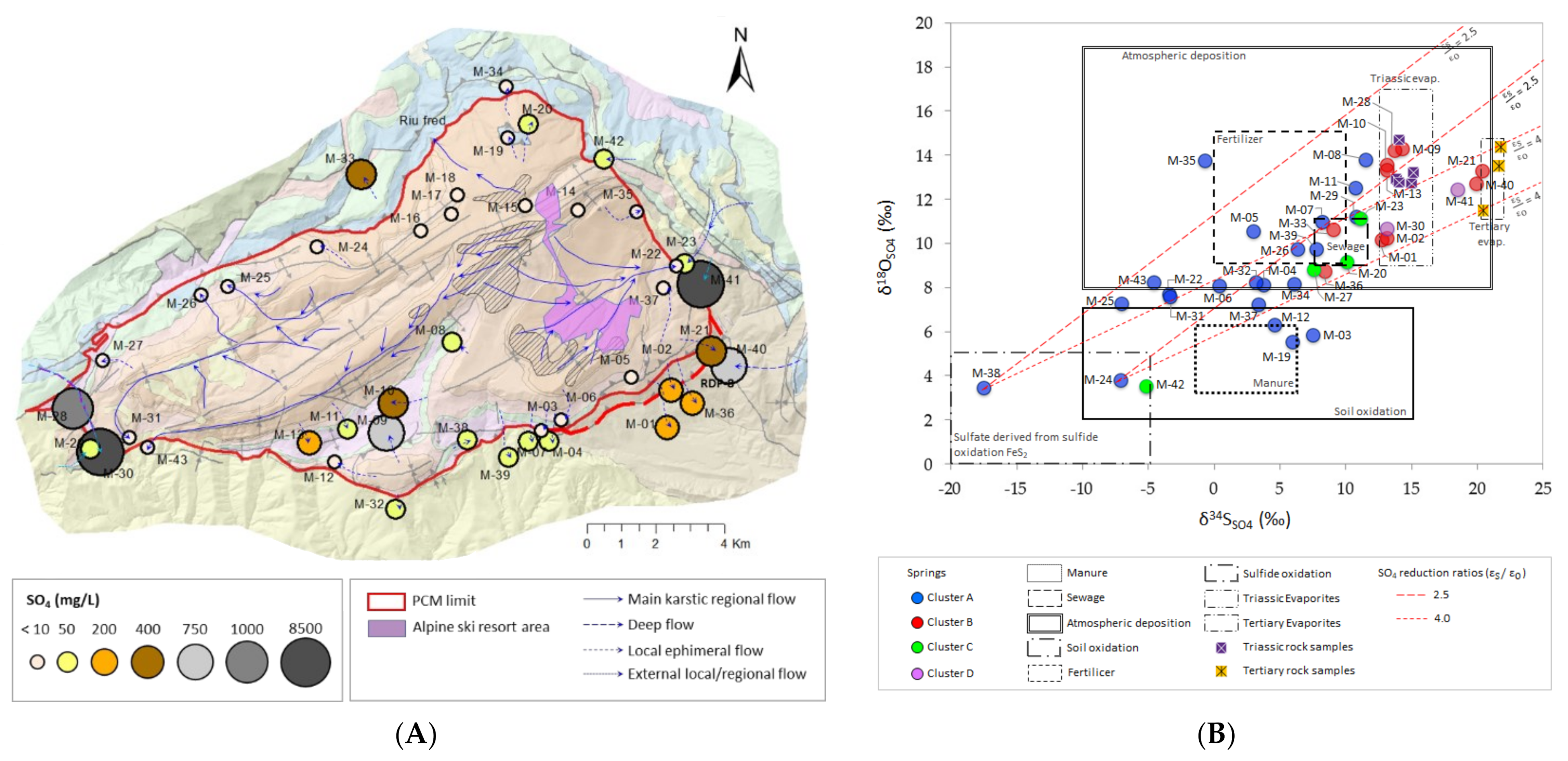
4.5. Identification of SO₄ Sources in GW Based on Stable Isotopes

To infer the origin of SO₄ in GW, the relationship between δ³⁴S_SO4 and δ¹⁸O_SO4 was considered for the different groundwater samples. In this analysis, the isotopic content obtained for the eight gypsum rock samples collected in the PCM area was included (Figure 9). The overall mean δ³⁴S_SO4 and mean δ¹⁸O_SO4 in GW are +6.5‰ and +9.5‰, respectively, with a large variation throughout the study area, between −17.5 and +20.4‰, and between +3.4 and +14.3‰, respectively. Based on the geological context, and supported by all available isotopic groundwater compositions, eight possible sources of SO₄ are considered: (1) Atmospheric deposition of SO₄ (Satm); (2) SO₄ derived from fertilizers (F); (3) SO₄ derived from sewage (Sew); (4) SO₄ derived manure (M); (5) SO₄ derived from soil (S); (6) SO₄ derived from weathering (oxidation) of sulfide minerals mainly related to Cretaceous carbonate rocks (SO); (7) dissolution of SO₄ from evaporites in the Triassic sequence (Tri); and (8) dissolution of SO₄ from evaporites in the Tertiary sequence (Ter).

Table 3. Mean δ³⁴S_SO4, δ¹⁸O_SO4, δ¹⁵N_NO3, and δ¹⁸O_NO3 isotopic content along with the sulfate and nitrate concentrations associated with the four GW clusters defined in the PCM.

	Cluster A	Cluster B	Cluster C	Cluster D
δ34SSO4 (‰)	+3.6	+13.2	+8.9	+15.9
δ18OSO4 (‰)	+8.1	+12.9	+8.9	+11.5
SO4 (mg/L)	6.9	213.3	11.5	4701
δ15NNO3 (‰)	+3.3	+3.8	+3.9	+8.6
δ18ONO3 (‰)	+2.9	+2.6	+1.4	+3.9
NO3 (mg/L)	10.1	16.8	10.4	5.6

shows the mean isotopic content by clusters. Table A6 and Table A7 Appendix A provide the average values for δ³⁴S_SO4 and δ¹⁸O_SO4 of samples available for all springs and the corresponding average SO₄ concentration and the data for the rock samples collected for the characterization of S and O sulfate isotopes content in Triassic and Tertiary gypsum in the PCM study area. Only groundwater samples from 38 springs out of a total of 48 could be considered in the analysis. No samples could be prepared for springs M-14, M-15, M-16, M-17, and M-18, which are associated with cluster A. These five springs are located at the highest part of the massif and present the lowest SO₄ content in groundwater.

The results suggest that the main source of SO₄ for cluster A might be related to all the factors, from pyrite oxidation to Beuda gypsum dissolution. Due to their intermediate isotopic composition, the role of atmospheric deposition, fertilizers, and sewage cannot be determined. Fertilizers have high sulphate contents [103,108] and cannot be discarded because they are applied in alpine ski resort areas to help the grass on the slopes reach maximum growth, and those applied in agricultural soils, which are planted with potato in some areas of the PCM. The sample with the lowest δ³⁴S_SO4 content (−17.5‰, in M-38 of Cluster A) is assumed to be, according to Municio (2017) [97], the result of sulfide mineral weathering. The spring M-38 is in the upper limit of the ‘sulphide oxidation field’ as defined by Van Stempvoort and Krouse (1994) [99]. Here, the sulfide minerals correspond to pyrites from marls with lignite materials, such as those appearing in the Upper Cretaceous—limestone-marl alternations and calcarenites (Kat, KMca) formations of the PCM.

The GW samples from Cluster B show a clear relationship with the Triassic (Keuper) window (M-09, M-10, M-28) and Tertiary window (Eocene-Oligocene Beuda’s gypsum Formation pinched out within the South Pyrenees thrust fault in the front SE of the PCM) (M-40, M-21), and partially mixed with soil inputs and atmospheric deposition (M-36 and M-33). Samples M-01 and M-02 are geologically affected by Tertiary gypsum. This has been observed directly in the field, so their position in the graph could be explained as a mixture of this source with soil sulfate.

The samples of cluster C are mostly related to Triassic evaporites but mixed with other sources. In the case of M-20 (cluster C), the isotopic content is consistent with the existence of a klippe of Triassic with Keuper outcropping, which affects the spring catchment, and with some contributions of fertilizers related to the cross-country (Nordic) ski resort, which is close to the spring. The isotopic composition of springs M-23 and M-42 suggests an origin in the soil. Nevertheless, in the case of M-42, there is an additional contribution of sulfate from atmospheric deposition.

The origin of the isotopic composition of the springs belonging to cluster D is related with the Triassic materials. The deep flow brine in spring M-30 matches perfectly inside the Triassic window, whereas the deep flow brine in spring M-41 falls between the Triassic and the Tertiary window, suggesting that the isotopic composition of this spring is affected by SO₄ contributions from these two origins. This is consistent with the structural geological context in which the spring M-41 is located, where the PCM and the Pedraforca thrust sheets coexist and are related to the ductile materials of the Keuper. As a result, the isotopic fingerprint of the Tertiary gypsum is added to that of the Triassic materials into the GW sampled in this spring.

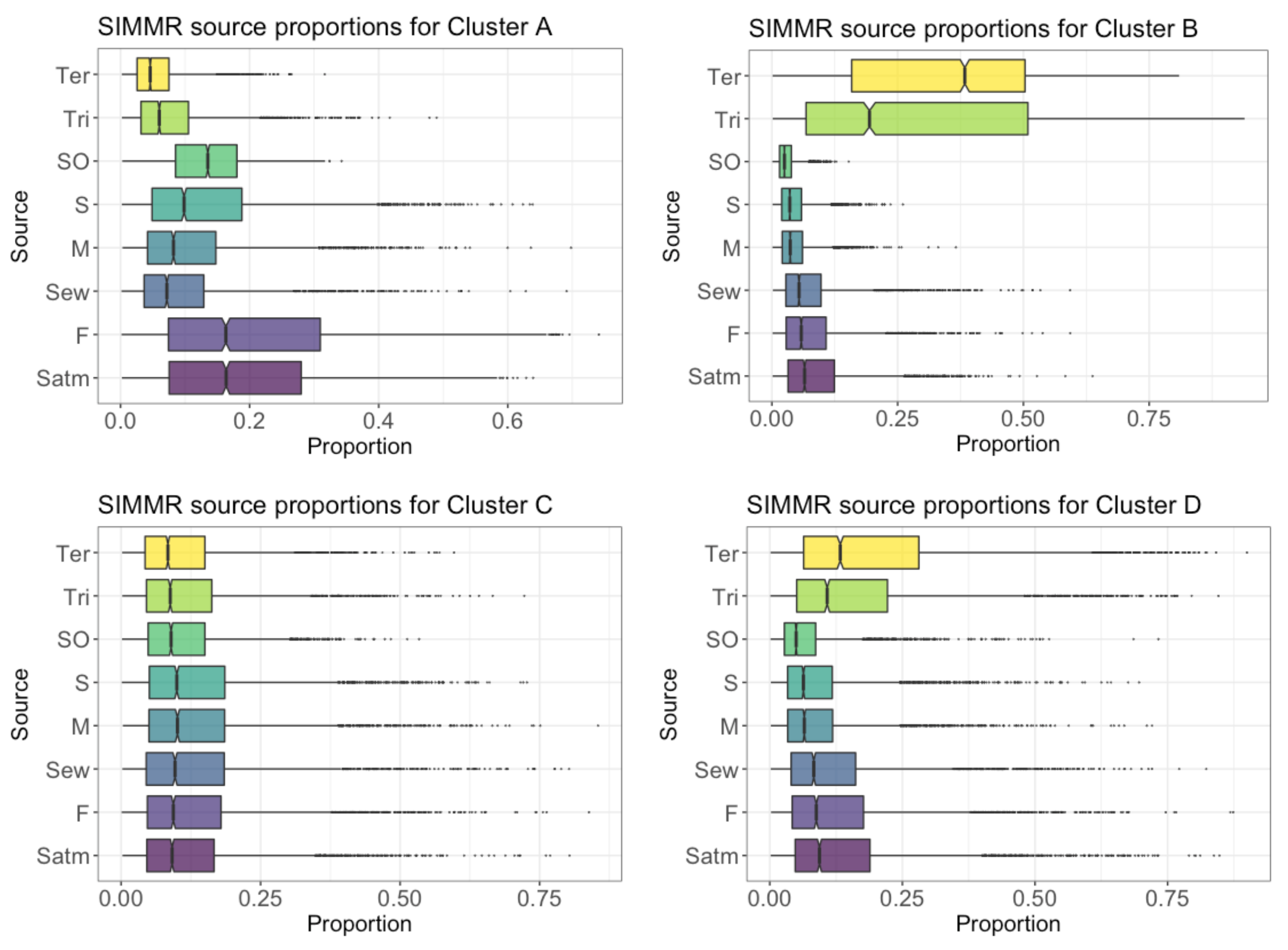
4.6. Proportional Contribution of SO₄ Sources in GW in the PCM

To enhance the existing knowledge regarding the sources of sulfate in groundwater, and to better explain the sources’ contribution, a Bayesian isotope mixing model was prepared using the SIMMR package for R (an updated version of the SIAR model [76,77]. Figure 10 presents the corresponding outputs aggregated for the four cluster A, B, C, and D with a horizontal boxplot showing the probabilistic contributions for each SO₄ source.

The results of the model indicate that the greatest contribution to springs associated with cluster A, which are mostly recharged in areas with little development of soil cover, comes from fertilizers (proportion~20.4%). They are probably related to their use in (1) the “Port del Comte” alpine ski resort, which is located near the top of the massif (Figure 11), an area that is drained by the four regional springs M-22, M-25, M-31, and M-43, and also other local springs, and (2) in the potato fields that are scattered throughout the massif. The atmospheric deposition also contributes (~18.9%), and finally sulfate from sulphide oxidation (~13.4%). For cluster B, the results confirm the clear effect of geogenic sulfate pollution, normally exceeding the drinking water limits > 250 mg/L of groundwater springs principally located at the lowest parts of the PCM. This is due to dissolution of Tertiary evaporites, mainly in the eastern part, with a mean proportion of ~ 34.4% with respect to the total sulfate contributions, and Triassic evaporites (~29.2%). In cluster C, the model shows a generalized mix of all eight sulfate sources considered, ranging between 10.8% and 13.7%. Regarding cluster D, which is composed of springs M-31 and M-41, the model also confirms that the origin of sulfate is mainly geogenic, related to Triassic and Tertiary evaporites with contributions between 16% and 19.6%. Figure A5, Appendix A, presents the model output for every spring. In relation to cluster A, the results obtained for the spring M-38 suggest that the contribution due to sulfide oxidation (64%) is consistent with the biplot shown in Figure 9B, and it is consistent with the field inspections, where the oxidation of sulphides associated with the Cretaceous limestones located in its drainage basin is observed. Another group of outstanding results from the Bayesian model are those associated with the springs belonging to cluster B, which are located at the eastern end of the PCM, an area where there is Tertiary gypsum outcrop. This is the case of the springs M-21, M-41, and M-40 that present a clear contribution, almost exclusive, from this source, with contributions of 85.2%, 78,1% and 89%, respectively.

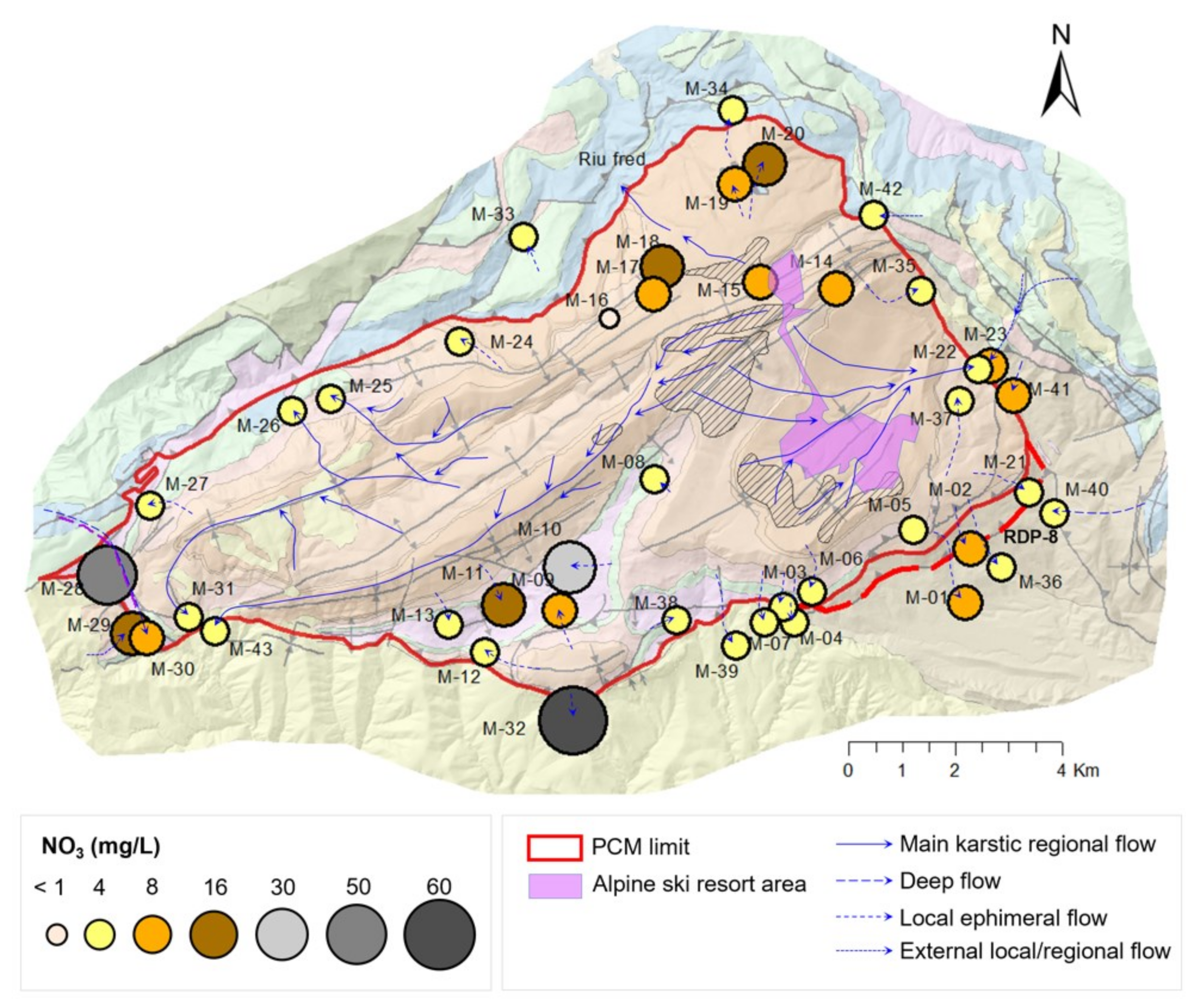
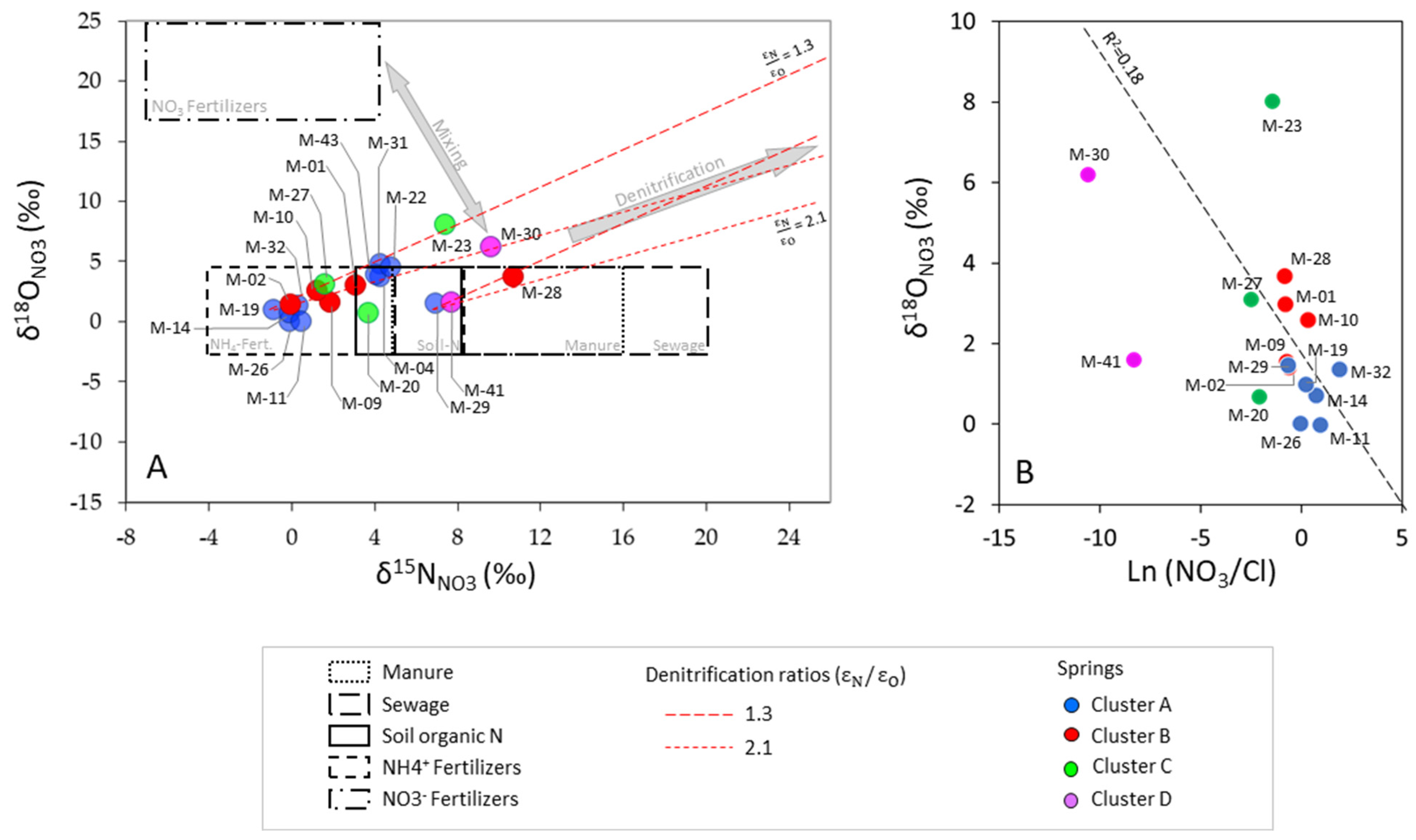
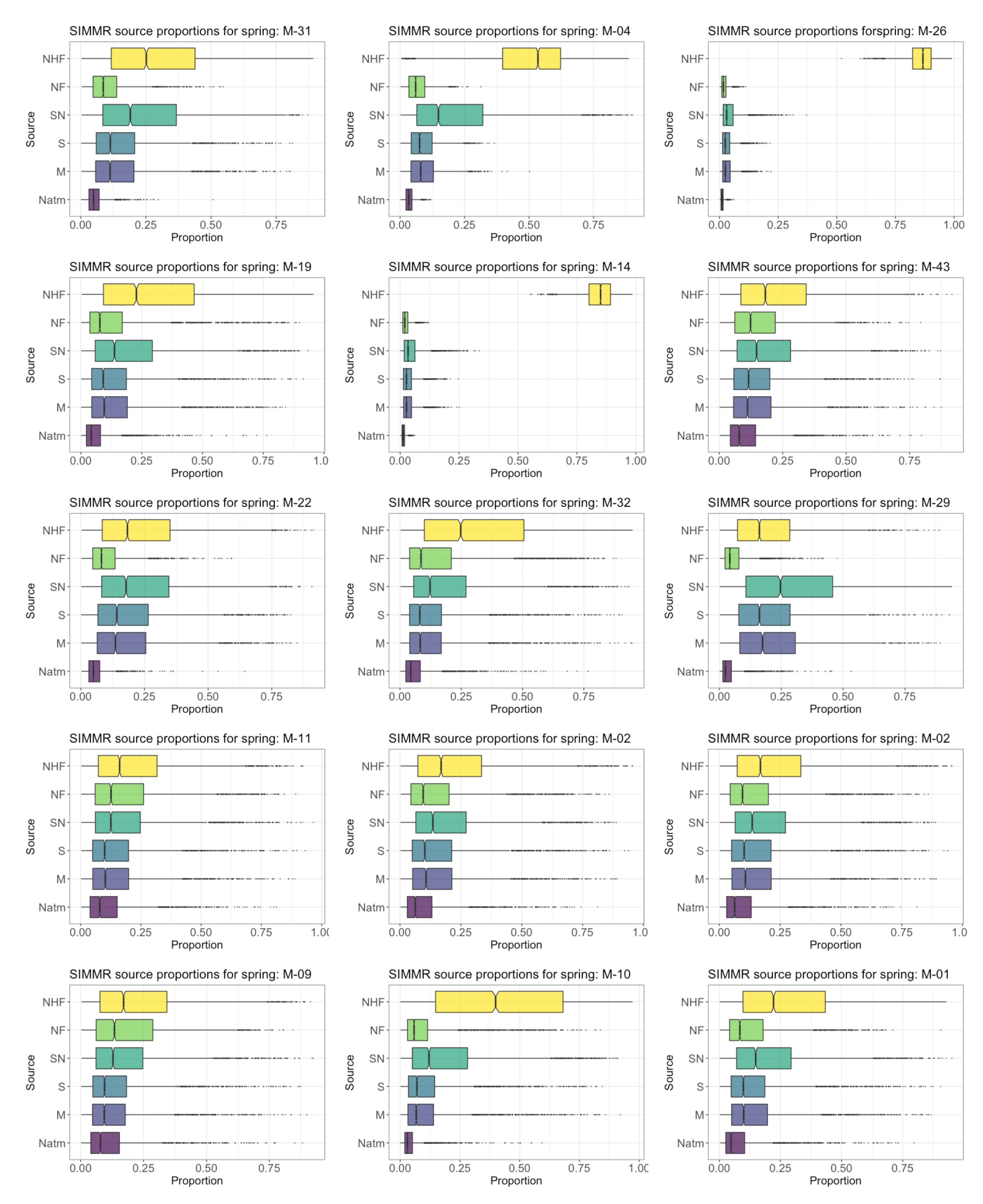
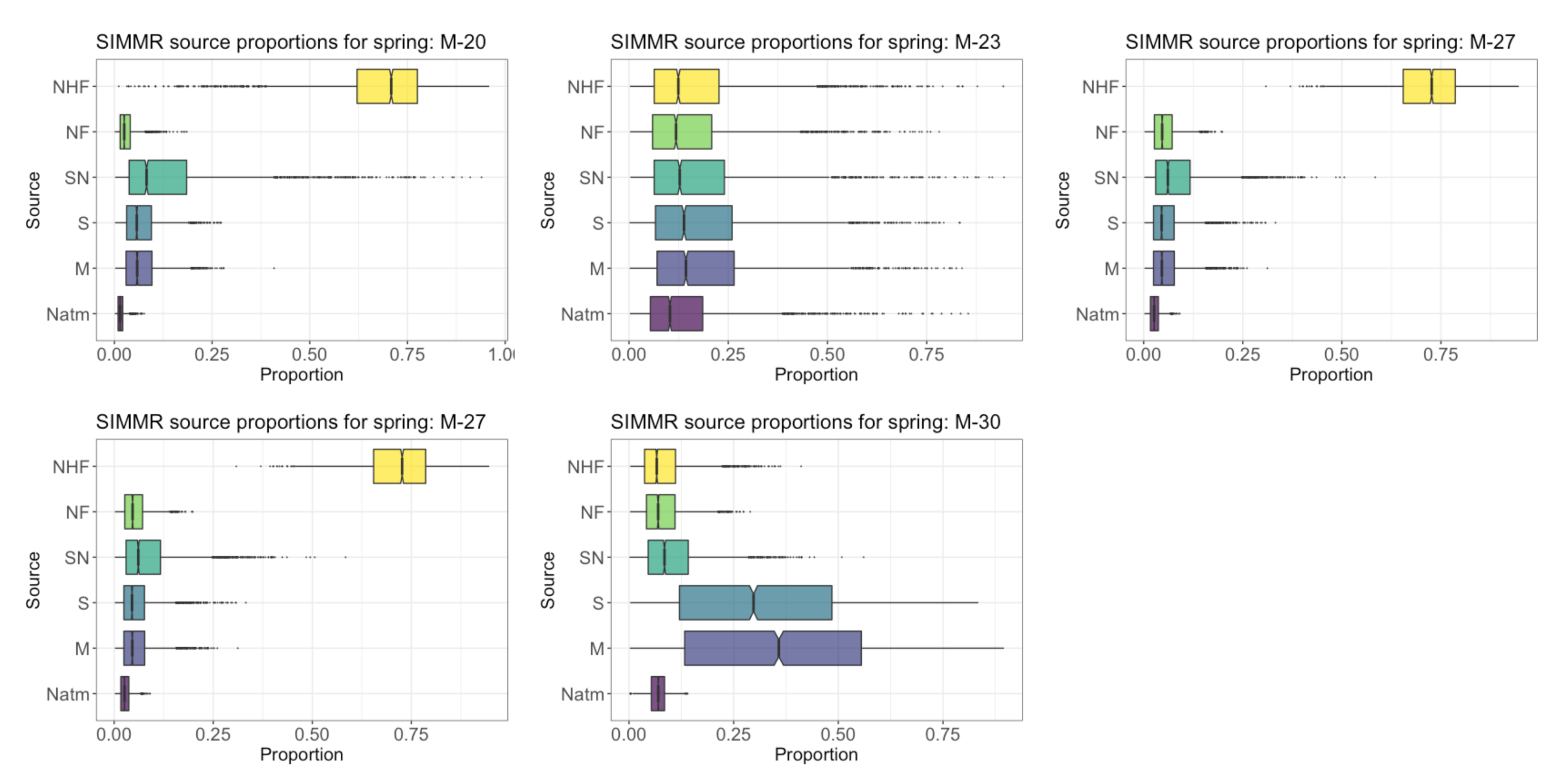
4.7. Identification of NO₃ Sources in GW and Perspectives on Aquifer Vulnerability in PCM

The most important N cycling reactions in lands are nitrification, mineralization-immobilization-turnover (MIT), plant uptake, denitrification, and NH₄ volatilization [109,110,111]. MIT refers to the recycling of NO₃ via immobilization as organic N, subsequent mineralization to NH₄ via organic matter degradation, and a turnover back to NO₃ via nitrification [111]. Immobilization, together with plant uptake, are two N assimilation pathways, which involve the production of organic N from inorganic compounds, such as NO₃, NO₂, or NH₄ [112].

The GW sampling campaigns revealed the existence of nitrate in some of the springs of the study area (Figure 11). With a median and a mean value of 3.83 and 7.13 mg/L, respectively, the nitrate content in GW does not seem to be a water quality issue in the PCM. Nevertheless, the spatial distribution of nitrate shows that the sources of nitrate may play a role locally. This is important when recharge is produced in a concentrated way, given that focused recharge facilitates the widespread, rapid incorporation and transport of pollutants to groundwater [3].

From the total 43 sampled springs, only 20 of them showed high enough nitrate concentrations in the GW samples to allow determination of the corresponding isotopic (δ¹⁵N_NO3 and δ¹⁸O_NO3) content (Figure 12A). The isotope content in GW ranges between −0.9‰ and +10.7‰ for δ¹⁵N_NO3, and between −0.0‰ and +8.2‰ for δ¹⁸O_NO3, with overall mean isotopic contents of +3.5‰ and +2.6‰ for δ¹⁵N_NO3 and δ¹⁸O_NO3, respectively. Table 3 shows both the mean nitrate and isotopic content by clusters.

Table A8Appendix A provides the average values for δ¹⁵N_NO3 and δ¹⁸O_NO3 of samples available of all springs and the corresponding average NO₃ concentration. The nitrate in GW seems to be unlinked to nitrate fertilizers, as the values of δ¹⁸O_NO3 and δ¹⁵N_NO3 in GW are far from the values of nitrate fertilizers (Figure 12A), although some mixing is not discarded. Nevertheless, NO₃ in GW appears to originate from soil organic nitrogen compounds, NH₄ fertilizers, sewage/manure sources, or even from a mixing of them. The highest NO₃ content value is 57.3 mg/L in spring M-32 (cluster A; Figure 11). This spring is located close to a potato crop field, where fertilizers are applied. This is consistent with the results obtained for δ¹⁸O_SO4 and δ³⁴S_SO4, which suggest the origin of SO₄ is a mixture of soil and fertilizer sulfate sources contributing to GW (Figure 9 and Figure A5, Appendix A for M-32). There is only one spring, M-28, whose H and O water isotopic composition presents the fingerprint of manure and sewage. In fact, this spring is neighbors a cattle farm where manure stocks are managed.

Concerning the δ¹⁸O_NO3 in the NO₃ from GW, its value depends on the δ¹⁸O of NO₃⁻ in water (−11.1‰, SD = 5.08‰) and on the isotopic effect produced during nitrification, which is in turn influenced by the +23.5‰ δ¹⁸O of dissolved atmospheric O₂ [113] and that of H₂O. The limited variation of δ¹⁸O_NO3 values along the study seems to indicate a negligible isotopic effect from plant uptake. Additionally, it indicates that denitrification processes were not significant along the studied area.

Most of the samples seem to follow a straight-line relationship between the δ¹⁵N and δ¹⁸O, with a factor between 1.3 and 2.1, which is consistent with natural denitrification [114] but with a slight variation. The natural denitrification process would be supported by the negative linear correlation between δ¹⁸O_NO3 and ln (NO₃/Cl) for the GW samples [115] (Figure 12B). Nevertheless, in the case of PCM, there is almost no correlation indicating that such a process, if it exists, is not significant.

The contamination of groundwater by nitrates in the PCM is mostly related to anthropic activities conducted in aquifer recharge areas. Here, the highest nitrate contents in GW are related to agricultural practices. Other relevant anthropic activities in the study area are restricted to those linked with the “Port del Comte” alpine ski resort. It is located near the top of the massif (Figure 11), in an area drained by the regional spring M-22, which is the most important resource of the PCM. Given the high karstification degree of the highest parts of the PCM, a hypothetical contamination coming from the ski resort would reach the aquifer feeding the spring M-22. Despite this, the impact of the sky resort in M-22 is not relevant at all, at least from the perspective of the NO₃ content in GW. This result stresses the good practices of the ski resort managers in terms of adopting measures to minimize the impact of such activity in the environment.

The dual-isotope diagram δ¹⁵N_NO3 vs. δ³⁴S_SO4 representing the isotopic composition of atmospheric deposition, soil, fertilizers, and sewage (Figure A7, Appendix A) for the water samples with both data available (i.e., δ¹⁵N_NO3 and δ³⁴S_SO4; a total of 19 springs) confirms that the main sources of groundwater pollution for springs belonging to cluster A, which are those discharging close to main recharge areas at the top of the PCM, are mainly the atmospheric deposition and fertilizers, and less the mineralization of soil organic matter. Nevertheless, in the case of the regional springs M-22, M-32, and M-43 (Figure 1), the oxidation of sulfides or organogenic sulfur appear to be an additional polluting source as pointed out by the BBM model. Besides, in the case of springs belonging to cluster B, there must be another contribution of sulfate, along with the atmospheric deposition, to explain their isotope content. According to the results of BMM, this source might be the sulfate of geogenic origin, due to the dissolution of Triassic and/or Tertiary gypsum.

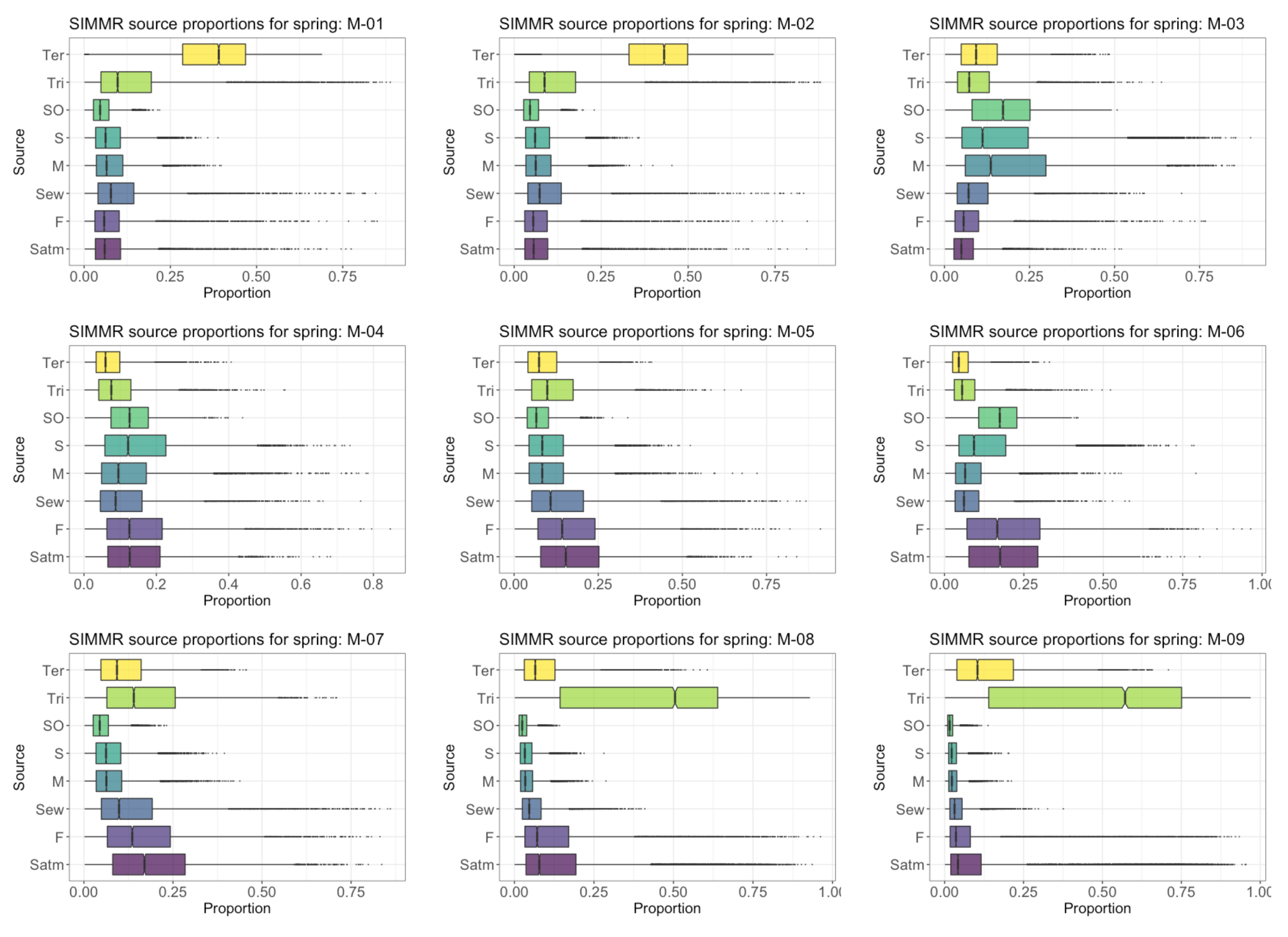
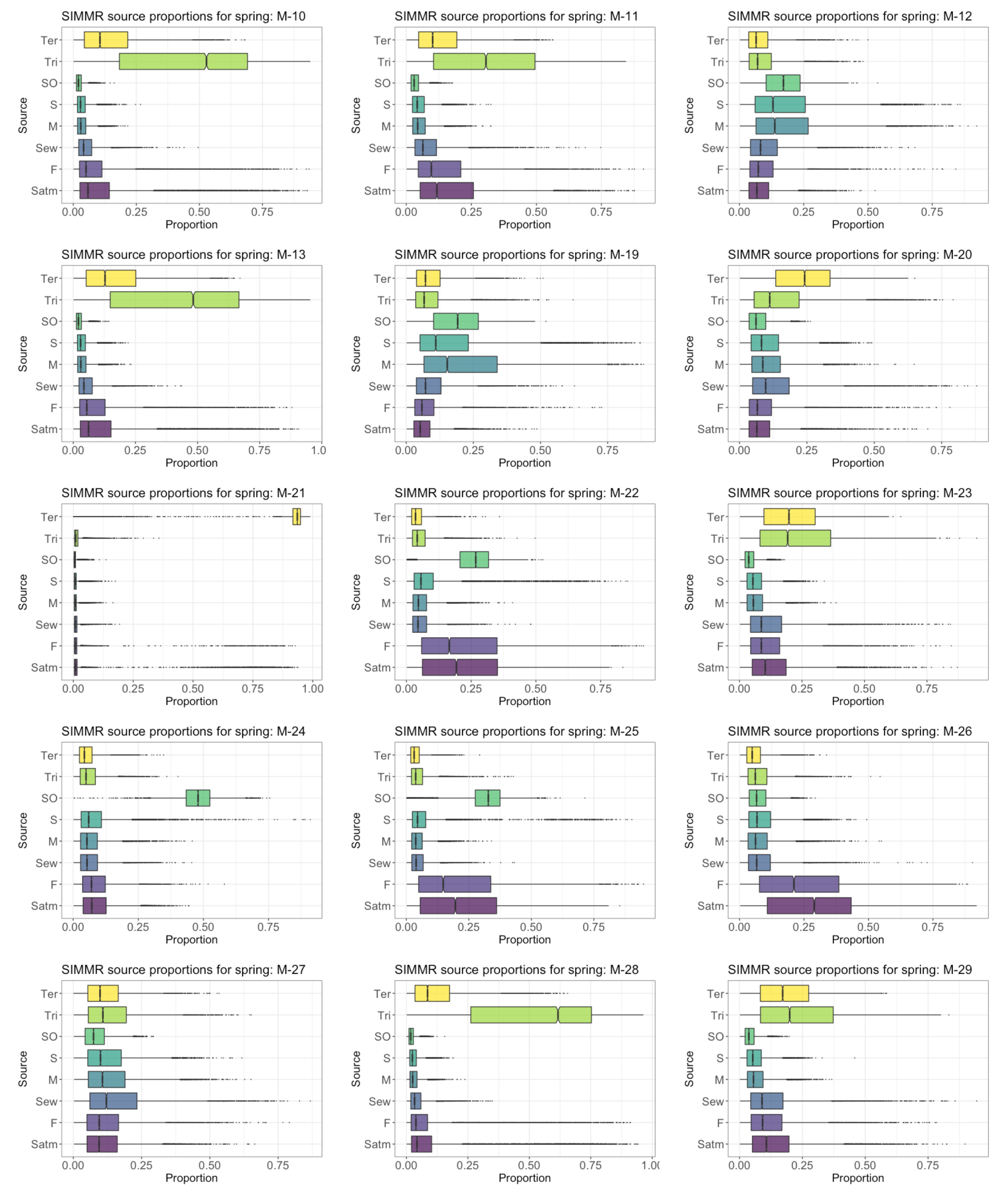
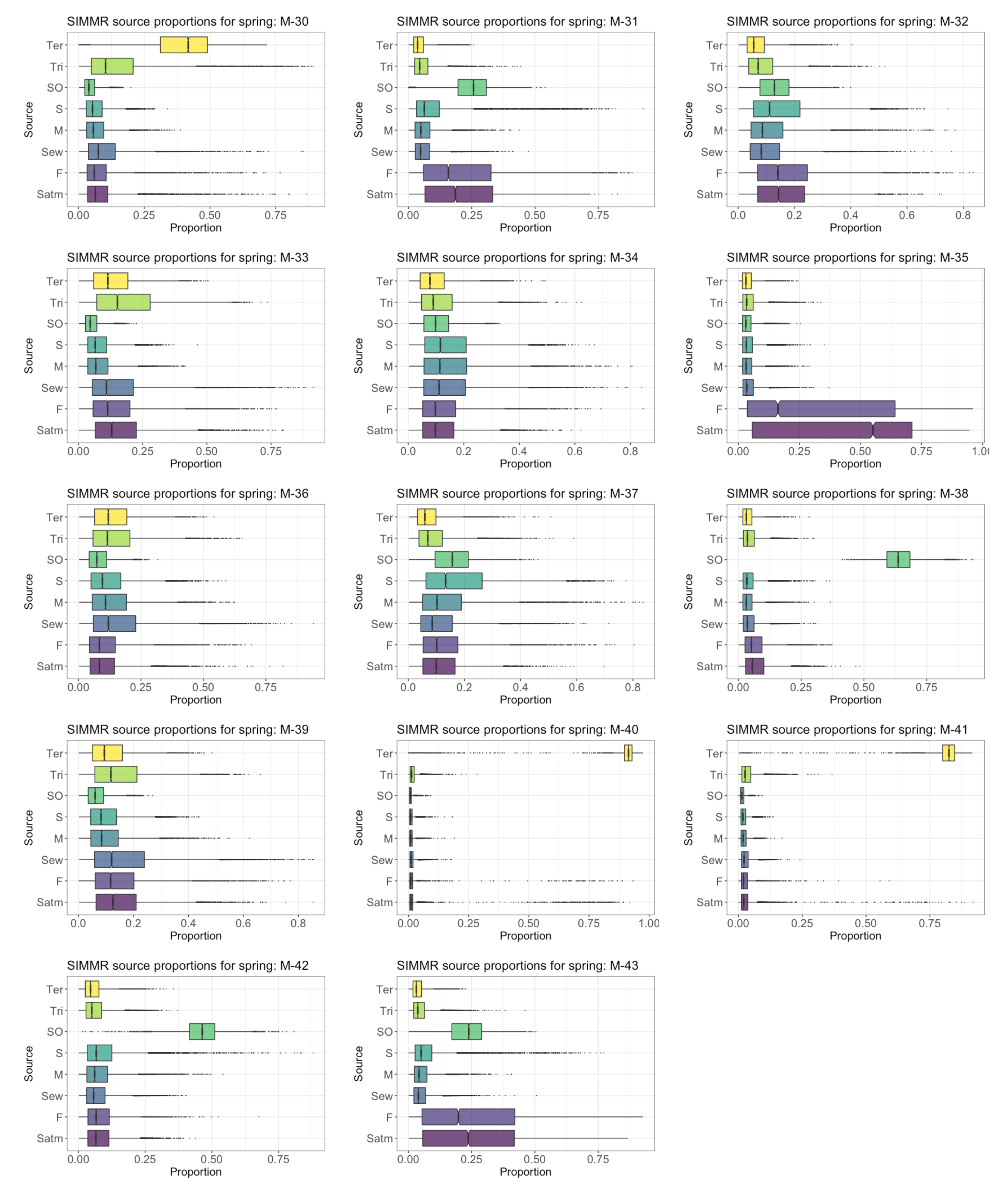
4.8. Proportional Contribution of NO₃ Sources in GW in PCM

A Bayesian isotope mixing model was prepared using the SIMMR package for R and was run to estimate proportional contributions of the NO₃ source for the 20 spring groundwater samples. The considered sources are the same as the biplots (Figure 12A) plus atmospheric deposition: (NHF) NO₃⁻ derived from NH₄⁺ in chemical fertilizers and precipitation; (NF) NO₃ in chemical fertilizer; (SN) soil organic nitrogen; (S) soil; (M) manure; and (Natm) atmospheric deposition. Figure A6, Appendix A, presents the corresponding outputs separated for each water spring.

The result of the model confirms that, in general, the greatest contribution of nitrates comes from pollution related to anthropic activities carried out in the aquifer recharge areas, mainly the use of fertilizers (NHF), except in a specific case with a notable proportion of manure (M) and sewage (S). Most springs have nitrate concentrations below current standards for drinking water. The only spring that exceeds the reference levels established at 50 ppm is the M-32 spring (with 57.3 ppm). This spring is located downstream of an area of field potato crops. The model indicates that it has an NHF proportion of 32%. The rest of the springs present similar or slightly higher NHF contributions although with lower nitrate concentrations. The second spring with the highest nitrate concentration corresponds to spring M-28 (38.6 ppm). In this case, the origin is clearly influenced by the livestock activity located upstream, presenting a proportion of 39.2% coming from manure and 31.7% coming from sewage.

4.9. Conceptual Model for Hydrogeochemical Evolution of GW in the PCM

From the combined analysis of the geological and hydrogeological context and chemical and isotopic data, global hydrogeological and hydrogeochemical conceptual models were interpreted based on the four cross-sections indicated in Figure 1.

The PCM is a high mountain karst aquifer, built upon several thrust sheets of carbonate materials. Precipitation is usually as snow in the highest part of the massif, where bare land abounds, along with the most developed karst forms in the epikarst (Figure 13 and Figure 14). The meteoric water from snowmelt and rainfall infiltrates and recharges the aquifer, mostly as Ca-Cl-HCO₃ type water. Recharged water flows in all directions and discharges through multiple significant springs. The main aquifer of the system is the one associated with the karstified limestones and dolostones of the Tertiary PPEc unit (Figure 1, Figure 13 and Figure 14), which underlies the PEcp1 and PEcp2 units.

The four most important springs in the system—named in decreasing discharge rate—are M-22 (in Figure 13A), M-25 and M-31 (in Figure 14B), and M-43 (see Figure 1). These springs drain the Tertiary karst aquifer along the syncline axes and were classified into cluster A by Herms et al. (2021) [59]. According to both their recharge elevation zones obtained with the H and O water isotopic content and the 3-D geological structure, these four springs present recharge-discharge pathways, several km long, while presenting a Ca-HCO₃ water type with low TDS (from 122 to 182 mg/L). These characteristics are interpreted as an indicator of a high karstification degree affecting the geological PPEc, PEcp1, and PEcp2 units, which favors large flow rates in both the percolating meteoric water through the unsaturated zone and the GW flow in the saturated zone. The hydrochemical signature of the GW flowing through the karst aquifer is obtained quickly, during the percolation and the first stages of the GW flow phases, as supported by the inverse modeling analysis done with the help of PHREEQC.

To illustrate this, Figure 13A shows the conceptual long RDP associated with the regional karst spring M-22. It includes a thick unsaturated zone and a regional water table level at elevations between 1000 and 1100 m a.s.l. Additionally, small and local springs, such as M-08 and M-05 (in Figure 13A), M-15 (in Figure 13B), or M-24 (in Figure 14A), drain the same karst aquifer and have a Ca-HCO₃ hydrochemical water type, with TDS mostly between 99 and 255 mg/L, and SO₄ coming from soil and atmospheric deposition, a composition which is similar to that of the regional springs. Additionally, the local springs may be affected by NH₄ fertilizers and/or manure. The discharge of springs located in the SE part of the study zone, which crosses the limits of the South Pyrenees thrust fault in the front SE of the PCM (right side of the Figure 13B), may be affected by Tertiary gypsum (PExb unit), generated by Ca-SO₄-HCO₃ to Ca-SO₄ water types.

Below the Tertiary limestone layers, the Garumnian Kgp unit acts as an aquitard, while the Upper Cretaceous Kat, KMca units, the Keuper Tk unit, and the Muschelkalk Tm unit (Triassic) act as local aquifers. These aquifer units drain through small local springs that may have been recharged through the overlying Tertiary carbonate units. The incoming recharge presents an initial Ca-HCO₃ signature, but it changes along the GW flow line by incorporating other solutes from the most soluble evaporite minerals in such local aquifers. There are some springs whose discharge present some hydrochemical special characteristics. Spring M-38 in cluster A (Figure 14A) interacts with lignite-bearing marls (KMca unit), incorporating sulfate from sulfide minerals (disseminated pyrites) or coal organic sulfur weathering, as is supported by the SO₄ isotope composition in groundwater; spring M-20 in cluster C incorporates Cl by dissolution of halite from the outcropping Keuper materials in the NE part of the massif (Figure 1). Additionally, Ca is dissolved by a reverse ion exchange-like process in weathering of shales, in which Na in dissolution replaces Ca in the terrain matrix. The springs that interact with the Keuper (Tk) unit, which are recharged either in the outcrops of this TK unit or through the geological units overlying it (e.g., Kgp, Kat, KMca), incorporate significant amounts of sulfate by dissolution of gypsum, as happens in springs M-10 (in Figure 13A and Figure 14A) and M-09 (Figure 14A). Both the S and O from the dissolved sulfate isotope composition and the inverse modeling with PHREEQC support this. Additionally, GW discharge may experience local de-dolomitization, as in the case of M-28 (see Figure 8), which presents the highest content of sulfate (Figure 9), thus inducing the precipitation of calcite, while those with deeper flow lines, such as springs M-30 (Figure 14B) and M-41 (see Figure 1) of cluster D, incorporate Cl and Na by dissolution of halite as well.

5. Conclusions

The Port del Comte Massif (PCM) contains one of the most important karst aquifers in the South-Eastern part of the Pyrenees. In this work, hydrochemical and multi-isotope data along with hydrogeological framework information were coupled to characterize the hydrochemical processes driving the hydrogeochemical behavior of this complex hydrogeological system.

In general, the groundwater is dominantly of the calcium bicarbonate and calcium–magnesium bicarbonate type, suggesting a dominant calcite dissolution process in agreement with the lithology associated with the Eocene carbonate materials conforming the main aquifer of PCM. The main source of sulfate in GW is the dissolution of geogenic origin from gypsum dissolution from the Eocene-Oligocene Beuda Formation and from Triassic evaporites. Some influence of sulfate from sulfide mineral or coal organic sulfur weathering was also indicated. From the anthropogenic point of view, sulphate from fertilizers seems to play a role in some places around the ski resort. Due to their intermediate values, the role of soil sulphate and sulphate from atmospheric deposition cannot be discarded. Isotope data showed that the source of recharge is precipitation that enters the system along the mountain slopes, favored by the high karstification of the carbonate materials that abundantly crop out in the area. Isotopes also show that dissolved NO₃ in groundwater mainly comes from mineral fertilizers, soil organic nitrogen, and pig manure application to the fields, with at most minor contributions from sewage. As the other high mountain karst systems, the PCM is very vulnerable to pollution. Here, nitrates from agricultural practices represent the main threat to the pristine waters of the aquifer system despite its low significance. Fortunately, the dissolved nitrate concentration in GW is generally low.

The carbonate karstic aquifer of the PCM is a very complex hydrological system developed in a high mountain environment. The multidisciplinary approach allowed the development of a hydrogeological conceptual model of aquifer system functioning, which is coherent with the available information from previous studies, but which is also consistent with the processes driving the hydrogeochemical and isotopic fingerprint of groundwater in this aquifer system.

References

1. Goldscheider, N.; Chen, Z.; Auler, A.S.; Bakalowicz, M.; Broda, S.; Drew, D.; Hartmann, J.; Jiang, G.; Moosdorf, N.; Stevanovic, Z.; et al. Global distribution of carbonate rocks and karst water resources. Hydrogeol. J. 2020, 28, 1661–1677. [Google Scholar] [CrossRef] [Green Version]
2. Parise, M.; Closson, D.; Gutiérrez, F.; Stevanović, Z. Anticipating and managing engineering problems in the complex karst environment. Environ. Earth Sci. 2015, 74, 7823–7835. [Google Scholar] [CrossRef]
3. Hartmann, A.; Jasechko, S.; Gleeson, T.; Wada, Y.; Andreo, B.; Barberá, J.A.; Brielmann, H.; Bouchaou, L.; Charlier, J.-B.; Darling, W.G.; et al. Risk of groundwater contamination widely underestimated because of fast flow into aquifers. Proc. Natl. Acad. Sci. USA 2021, 118, e2024492118. [Google Scholar] [CrossRef] [PubMed]
4. Hock, R.; Rasul, G.; Adler, C.; Cáceres, B.; Gruber, S.; Hirabayashi, Y.; Jackson, M.; Kääb, A.; Kang, S.; Kutuzov, S.; et al. 2019: High mountain areas. In IPCC Special Report on the Ocean and Cryosphere in a Changing Climate; Pörtner, H.-O., Roberts, D.C., Masson-Delmotte, V., Zhai, P., Tignor, M., Poloczanska, E., Mintenbeck, K., Alegría, A., Nicolai, M., Okem, A., et al., Eds.; IPCC—Intergovernmental Panel on Climate Change: Geneva, Switzerland, 2019; pp. 131–202. Available online: http://urn.kb.se/resolve?urn=urn:nbn:se:uu:diva-414230. (accessed on 1 June 2021).
5. Jódar, J.; Lambán, L.J.; González, A.; Martos, S.; Custodio, E. High Mountain Karst Aquifer Vulnerability to Climate Change and Groundwater Transit Times. In Proceedings of the EGU General Assembly 2020, Online, 4–8 May 2020. [Google Scholar] [CrossRef]
6. Jódar, J.; Herms, I.; Lambán, L.J.; Martos-Rosillo, S.; Herrera-Lameli, C.; Urrutia, J.; Soler, A.; Custodio, E. Isotopic content in high mountain karst aquifers as a proxy for climate change impact in Mediterranean zones: The Port del Comte karst aquifer (SE Pyrenees, Catalonia, Spain). Sci. Total Environ. 2021, 790, 148036. [Google Scholar] [CrossRef]
7. Lambán, L.J.; Jódar, J.; Custodio, E.; Soler, A.; Sapriza, G.; Soto, R. Isotopic and hydrogeochemical characterization of high-altitude karst aquifers in complex geological settings. The Ordesa and Monte Perdido National Park (Northern Spain) case study. Sci. Total Environ. 2015, 506–507, 466–479. [Google Scholar] [CrossRef] [Green Version]
8. Sheikhy Narany, T.; Bittner, D.; Disse, M.; Chiogna, G. Spatial and temporal variability in hydrochemistry of a small-scale dolomite karst environment. Environ. Earth Sci. 2019, 78, 273. [Google Scholar] [CrossRef]
9. Mudarra, M.; Andreo, B.; Mudry, J. Monitoring groundwater in the discharge area of a complex karst aquifer to assess the role of the saturated and unsaturated zones. Environ. Earth Sci. 2012, 65, 2321–2336. [Google Scholar] [CrossRef]
10. Montalván, F.J.; Heredia, J.; Ruiz, J.M.; Pardo-Igúzquiza, E.; García de Domingo, A.; Elorza, F.J. Hydrochemical and isotopes studies in a hypersaline wetland to define the hydrogeological conceptual model: Fuente de Piedra Lake (Málaga, Spain). Sci. Total Environ. 2017, 576, 335–346. [Google Scholar] [CrossRef]
11. Apollaro, C.; Fuoco, I.; Bloise, L.; Calabrese, E.; Marini, L.; Vespasiano, G.; Muto, F. Geochemical modeling of water-rock interaction processes in the Pollino National Park. Geofluids 2021, 2021, 6655711. [Google Scholar] [CrossRef]
12. Goldscheider, N. Overview of methods applied in karst hydrogeology. In Karst Aquifers—Characterization and Engineering; Professional Practice in Earth Sciences Series; Stevanović, Z., Ed.; Springer International Publishing: Cham, Switzerland, 2015; pp. 127–145. ISBN 978-3-319-12849-8. [Google Scholar]
13. Simsek, C.; Elci, A.; Gunduz, O.; Erdogan, B. Hydrogeological and hydrogeochemical characterization of a karstic mountain region. Environ. Geol. 2008, 54, 291–308. [Google Scholar] [CrossRef]
14. Mustafa, O.; Merkel, B.; Weise, S. Assessment of Hydrogeochemistry and environmental isotopes in karst springs of Makook anticline, Kurdistan Region, Iraq. Hydrology 2015, 2, 48–68. [Google Scholar] [CrossRef] [Green Version]
15. Guo, Y.; Zhang, C.; Xiao, Q.; Bu, H. Hydrogeochemical characteristics of a closed karst groundwater basin in North China. J. Radioanal. Nucl. Chem. 2020, 325, 365–379. [Google Scholar] [CrossRef]
16. De la Torre, B.; Mudarra, M.; Andreo, B. Investigating karst aquifers in tectonically complex alpine areas coupling geological and hydrogeological methods. J. Hydrol. X 2020, 6, 100047. [Google Scholar] [CrossRef]
17. Farlin, J.; Małoszewski, P. On using lumped parameter models and temperature cycles in heterogeneous aquifers. Groundwater 2018, 56, 969–977. [Google Scholar] [CrossRef]
18. Jódar, J.; Custodio, E.; Lambán, L.J.; Martos-Rosillo, S.; Herrera-Lameli, C.; Sapriza-Azuri, G. Vertical variation in the amplitude of the seasonal isotopic content of rainfall as a tool to jointly estimate the groundwater recharge zone and transit times in the Ordesa and Monte Perdido National Park Aquifer System, North-Eastern Spain. Sci. Total Environ. 2016, 573, 505–517. [Google Scholar] [CrossRef] [Green Version]
19. Jódar, J.; González-Ramón, A.; Martos-Rosillo, S.; Heredia, J.; Herrera, C.; Urrutia, J.; Caballero, Y.; Zabaleta, A.; Antigüedad, I.; Custodio, E.; et al. Snowmelt as a determinant factor in the hydrogeological behaviour of high mountain karst aquifers: The Garcés Karst System, Central Pyrenees (Spain). Sci. Total Environ. 2020, 748, 141363. [Google Scholar] [CrossRef] [PubMed]
20. Díaz-Puga, M.A.; Vallejos, A.; Sola, F.; Daniele, L.; Molina, L.; Pulido-Bosch, A. Groundwater flow and residence time in a karst aquifer using ion and isotope characterization. Int. J. Environ. Sci. Technol. 2016, 13, 2579–2596. [Google Scholar] [CrossRef]
21. Gao, Z.; Liu, J.; Xu, X.; Wang, Q.; Wang, M.; Feng, J.; Fu, T. Temporal variations of spring water in karst areas: A case study of Jinan Spring Area, Northern China. Water 2020, 12, 1009. [Google Scholar] [CrossRef] [Green Version]
22. Safari, M.; Hezarkhani, A.; Mashhadi, S.R. Hydrogeochemical characteristics and water quality of Aji-Chay River, Eastern Catchment of Lake Urmia, Iran. J. Earth Syst. Sci. 2020, 129, 199. [Google Scholar] [CrossRef]
23. Chalikakis, K.; Plagnes, V.; Guerin, R.; Valois, R.; Bosch, F.P. Contribution of geophysical methods to karst-system exploration: An overview. Hydrogeol. J. 2011, 19, 1169–1180. [Google Scholar] [CrossRef]
24. Jia, Z.; Zang, H.; Hobbs, P.; Zheng, X.; Xu, Y.; Wang, K. Application of inverse modeling in a study of the hydrogeochemical evolution of karst groundwater in the Jinci Spring Region, Northern China. Environ. Earth Sci. 2017, 76, 312. [Google Scholar] [CrossRef]
25. Moran-Ramírez, J.; Ramos-Leal, J.A.; Mahlknecht, J.; Santacruz-DeLeón, G.; Martín-Romero, F.; Fuentes Rivas, R.; Mora, A. Modeling of groundwater processes in a karstic aquifer of Sierra Madre Oriental, Mexico. Appl. Geochem. 2018, 95, 97–109. [Google Scholar] [CrossRef]
26. Zheng, X.; Zang, H.; Zhang, Y.; Chen, J.; Zhang, F.; Shen, Y. A study of hydrogeochemical processes on karst groundwater using a mass balance model in the Liulin Spring Area, North China. Water 2018, 10, 903. [Google Scholar] [CrossRef] [Green Version]
27. Pérez-Ceballos, R.; Canul-Macario, C.; Pacheco-Castro, R.; Pacheco-Ávila, J.; Euán-Ávila, J.; Merino-Ibarra, M. Regional hydrogeochemical evolution of groundwater in the ring of cenotes, Yucatán (Mexico): An Inverse Modelling Approach. Water 2021, 13, 614. [Google Scholar] [CrossRef]
28. Chen, Z.; Goldscheider, N. Modeling spatially and temporally varied hydraulic behavior of a folded karst system with dominant conduit drainage at catchment scale, Hochifen–Gottesacker, Alps. J. Hydrol. 2014, 514, 41–52. [Google Scholar] [CrossRef]
29. Herms, I.; Jódar, J.; Soler, A.; Vadillo, I.; Lambán, L.J.; Martos-Rosillo, S.; Núñez, J.A.; Arnó, G.; Jorge, J. Contribution of isotopic research techniques to characterize high-mountain-Mediterranean karst aquifers: The Port del Comte (Eastern Pyrenees) aquifer. Sci. Total Environ. 2019, 656, 209–230. [Google Scholar] [CrossRef]
30. Betzler, C. A Carbonate complex in an active foreland basin: The Paleogene of the Sierra de Port del Comte and the Sierra del Cadi (Southern Pyrenees). Geodin. Acta 1989, 3, 207–220. [Google Scholar] [CrossRef]
31. Vergès i Masip, J. Estudi Geològic del Vessant Sud del Pirineu Oriental i Central. Evolució Cinemàtica en 3D; Universitat de Barcelona UB: Barcelona, Spain, 1993. [Google Scholar]
32. Barcelona City Council. Evolution of Water Consumption in the City of Barcelona; Barcelona City Council: Barcelona, Spain, 2008.
33. Herms, I. 3D geological modelling as a tool for supporting spring catchment delineation in high-mountain karst aquifers: The case study of the Port Del Comte (Eastern Pyrenees) Aquifer. In Proceedings of the 5th European Meeting on 3D Geological Modelling, Bern, Switzerland, 21–24 May 2019. [Google Scholar]
34. Arnó, G.; Conesa, A.; Carreras, X.; Camps, V.; Fraile, J.; Herms, I.; Iglesias, M. Mapa de Vulnerabilitat Intrínseca a la Contaminació dels Aqüífers de Catalunya (MVIAC) 2020, Escala 1:100.000. Barcelona. Institut Cartogràfic i Geològic de Catalunya (ICGC) i Agència Catalana de l’Aigua (ACA). Available online: https://www.icgc.cat/ca/Administracio-i-empresa/Eines/Visualitzadors-Geoindex/Geoindex-Vulnerabilitat-intrinseca-a-la-contaminacio-dels-aqueifers (accessed on 15 January 2021).
35. DARP. Proyecto de Prospección e Investigación Hidrogeológica (Solsonès–Lleida); DARP (Departament d’Agricultura, Ramaderia i Pesca, Generalitat de Catalunya): Barcelona, Spain, 1990; pp. 20–117.
36. Gil, R.; Núñez, I. Estudio Hidrogeológico de la Sierra de Odén–Port del Comte (Solsonès–Lleida); CIHS: Barcelona, Spain, 2003; p. 85. [Google Scholar]
37. Núñez, I.; Gil, R.; Vázquez, E. Estudio hidrogeológico de la cabecera de la Ribera Salada, (Lleida). In Proceedings of the VIII Simposio de Hidrogeología, Zaragoza, Spain, 18–22 October 2004; pp. 107–120. [Google Scholar]
38. Chen, Z.; Hartmann, A.; Wagener, T.; Goldscheider, N. Dynamics of water fluxes and storages in an alpine karst catchment under current and potential future climate conditions. Hydrol. Earth Syst. Sci. 2018, 22, 3807–3823. [Google Scholar] [CrossRef] [Green Version]
39. Pardo-Igúzquiza, E.; Collados-Lara, A.J.; Pulido-Velàzquez, D. Potential future impact of climate change on recharge in the Sierra de Las Nieves (Southern Spain) high-relief karst aquifer using regional climate models and statistical corrections. Environ. Earth Sci. 2019, 78, 598. [Google Scholar] [CrossRef]
40. Peel, M.C.; Finlayson, B.L.; McMahon, T.A. Updated world map of the Köppen-Geiger climate classification. Hydrol. Earth Syst. Sci. 2007, 11, 1633–1644. [Google Scholar] [CrossRef] [Green Version]
41. ICGC. Full Alt Urgell. Mapa Geològic Comarcal de Catalunya 1:50.000. 2007. Available online: https://www.icgc.cat/en/Public-Administration-and-Enterprises/Downloads/Geological-and-geothematic-cartography/Geological-cartography/Geological-map-1-50-000/Regional-geological-map-of-Catalonia-1-50-000 (accessed on 10 January 2021).
42. Lauber, U.; Kotyla, P.; Morche, D.; Goldscheider, N. Hydrogeology of an alpine rockfall aquifer system and its role in flood attenuation and maintaining baseflow. Hydrol. Earth Syst. Sci. 2014, 18, 4437–4452. [Google Scholar] [CrossRef] [Green Version]
43. Hood, J.L.; Hayashi, M. Assessing the Application of a laser rangefinder for determining snow depth in inaccessible alpine terrain. Hydrol. Earth Syst. Sci. 2010, 14, 901–910. [Google Scholar] [CrossRef] [Green Version]
44. Goldscheider, N. Alpine hydrogeologie. Grundwasser 2011, 16, 1. [Google Scholar] [CrossRef] [Green Version]
45. Bakalowicz, M. Karst groundwater: A challenge for new resources. Hydrogeol. J. 2005, 13, 148–160. [Google Scholar] [CrossRef]
46. Goldscheider, N.; Drew, D. Methods in karst hydrogeology. In International Contributions to Hydrogeology 26; Taylor&Francis: London, UK, 2007; ISBN 978-0-415-42873-6. [Google Scholar]
47. Wetzel, K.-F. On the hydrology of the partnach area in the Wetterstein Mountains (Bavarian Alps). Erdkunde 2004, 58, 172–186. [Google Scholar] [CrossRef]
48. Malard, A.; Sinreich, M.; Jeannin, P.-Y. A novel approach for estimating karst groundwater recharge in mountainous regions and its application in Switzerland: Karst groundwater recharge: Approach and application. Hydrol. Process. 2016, 30, 2153–2166. [Google Scholar] [CrossRef]
49. Epting, J.; Page, R.M.; Auckenthaler, A.; Huggenberger, P. Process-based monitoring and modeling of karst springs–linking intrinsic to specific vulnerability. Sci. Total Environ. 2018, 625, 403–415. [Google Scholar] [CrossRef] [PubMed]
50. Jódar, J.; Custodio, E.; Liotta, M.; Lambán, L.J.; Herrera, C.; Martos-Rosillo, S.; Sapriza, G.; Rigo, T. Correlation of the seasonal isotopic amplitude of precipitation with annual evaporation and altitude in alpine regions. Sci. Total Environ. 2016, 550, 27–37. [Google Scholar] [CrossRef] [PubMed]
51. Beven, K.J. Rainfall-Runoff Modelling, The Primer, 2nd ed.; Wiley-Blackwell: Chichester, UK, 2012; ISBN 978-0-470-71459-1. [Google Scholar]
52. Andreo, B.; Liñán, C.; Carrasco, F.; Jiménez de Cisneros, C.; Caballero, F.; Mudry, J. Influence of rainfall quantity on the isotopic composition (18O and 2H) of water in mountainous areas. application for groundwater research in the Yunquera-Nieves Karst Aquifers (S Spain). Appl. Geochem. 2004, 19, 561–574. [Google Scholar] [CrossRef]
53. Bergström, S. Development and Application of a Conceptual Runoff Model for Scandinavian Catchments; SMHI: Norrköping, Sweden, 1976; p. 134. [Google Scholar]
54. Seibert, J. HBV Light Version 2. User’s Manual; Stockholm University: Uppsala, Sweden, 2005. [Google Scholar]
55. Małoszewski, P.; Zuber, A. Lumped Parameter Models for the Interpretation of Environmental Tracer Data. Manual on Mathematical Models in Isotope Hydrology; IAEA: Vienna, Austria, 1996. [Google Scholar]
56. Maréchal, J.C.; Bailly-Comte, V.; Hickey, C.; Maurice, L.; Stroj, A.; Bunting, S.Y.; Charlier, J.B.; Elster, D.; Hakoun, V.; Herms, I.; et al. GeoERA Resources of Groundwater Harmonized at Cross-Border and Pan-European Scale (RESOURCE) Project’. Deliverable 5.3 Karst and Chalk Aquifers Classification and Management Recommendations; BRGM: Toulousse, France, 2021; p. 114. [Google Scholar]
57. Mangin, A. Contribution à L’étude Hydrodynamique des Aquifères Karstiques; Université de Dijon: Dijon, France, 1975. [Google Scholar]
58. Freixes, A. Els Aqüífers Càrstics dels Pirineus de Catalunya. Interès Estratègic i Sostenibilitat; Universitat de Barcelona UB: Barcelona, Spain, 2014. [Google Scholar]
59. Herms, I.; Jódar, J.; Soler, A.; Lambán, L.J.; Custodio, E.; Núñez, J.A.; Arnó, G.; Ortego, M.I.; Parcerisa, D.; Jorge, J. Evaluation of natural background levels of high mountain karst aquifers in complex hydrogeological settings. A gaussian mixture model approach in the Port del Comte (SE, Pyrenees) case study. Sci. Total Environ. 2021, 756, 143864. [Google Scholar] [CrossRef] [PubMed]
60. Fraley, C.; Raftery, A.E. Model-based clustering, discriminant analysis, and density estimation. J. Am. Stat. Assoc. 2002, 97, 611–631. [Google Scholar] [CrossRef]
61. Bouveyron, C.; Brunet-Saumard, C. Model-based clustering of high-dimensional data: A review. Comput. Stat. Data Anal. 2014, 71, 52–78. [Google Scholar] [CrossRef] [Green Version]
62. Camarero, L.; Catalan, J. Chemistry of bulk precipitation in the Central and Eastern Pyrenees, Northeast Spain. Atmos. Environ. Part Gen. Top. 1993, 27, 83–94. [Google Scholar] [CrossRef]
63. Bergström, S. The HBV Model–Its Structure and Applications; Reports Hydrology; SMHI: Norrkoping, Sweden, 1992. [Google Scholar]
64. Alcalá, F.J.; Custodio, E. Atmospheric chloride deposition in continental Spain. Hydrol. Process. 2008, 22, 3636–3650. [Google Scholar] [CrossRef]
65. Coplen, T.B. Guidelines and recommended terms for expression of stable-isotope-ratio and gas-ratio measurement results: Guidelines and recommended terms for expressing stable isotope results. Rapid Commun. Mass Spectrom. 2011, 25, 2538–2560. [Google Scholar] [CrossRef] [PubMed]
66. Wassenaar, L.I.; Ahmad, M.; Aggarwal, P.; Duren, M.; Pöltenstein, L.; Araguas, L.; Kurttas, T. Worldwide proficiency test for routine analysis of δ2H and δ 18O in water by isotope-ratio mass spectrometry and laser absorption spectroscopy: Proficiency Test for δ 2H and δ 18O in natural waters. Rapid Commun. Mass Spectrom. 2012, 26, 1641–1648. [Google Scholar] [CrossRef]
67. Epstein, S.; Mayeda, T. Variation of O18 content of waters from natural sources. Geochim. Cosmochim. Acta 1953, 4, 213–224. [Google Scholar] [CrossRef]
68. McIlvin, M.R.; Altabet, M.A. Chemical conversion of nitrate and nitrite to nitrous oxide for nitrogen and oxygen isotopic analysis in freshwater and seawater. Anal. Chem. 2005, 77, 5589–5595. [Google Scholar] [CrossRef]
69. Dogramaci, S.S.; Herczeg, A.L.; Schi, S.L.; Bone, Y. Controls on δ 34S and δ18O of dissolved sulfate in aquifers of the Murray basin, Australia and their use as indicators of flow processes. Appl. Geochem. 2001, 14, 475–488. [Google Scholar] [CrossRef]
70. Parkhurst, D.L.; Appelo, C.A.J. Description of Input and Examples for PHREEQC Version 3—A Computer Program for Speciation, Batch-Reaction, One-Dimensional Transport, and Inverse Geochemical Calculations; U.S. Geological Survey Techniques and Methods: Reston, VA, USA, 2013; Book 6, Chapter A43; p. 497.
71. Appelo, C.A.J.; Postma, D. Geochemistry, Groundwater and Pollution, 2nd ed.; CRC Press: London, UK, 2005. [Google Scholar]
72. Puig, R.; Folch, A.; Menció, A.; Soler, A.; Mas-Pla, J. Multi-isotopic study (15N, 34S, 18O, 13C) to identify processes affecting nitrate and sulfate in response to local and regional groundwater mixing in a large-scale flow system. Appl. Geochem. 2013, 32, 129–141. [Google Scholar] [CrossRef]
73. Puig, R.; Soler, A.; Widory, D.; Mas-Pla, J.; Domènech, C.; Otero, N. Characterizing sources and natural attenuation of nitrate contamination in the Baix Ter Aquifer System (NE Spain) using a multi-isotope approach. Sci. Total Environ. 2017, 580, 518–532. [Google Scholar] [CrossRef] [PubMed]
74. Kendall, C.; McDonnell, J.J. Tracing nitrogen sources and cycling in catchments. In Isotope Tracers in Catchment Hydrology; Elsevier: Amsterdam, The Netherlands, 1998; pp. 519–576. [Google Scholar] [CrossRef]
75. Xue, D.; De Baets, B.; Van Cleemput, O.; Hennessy, C.; Berglund, M.; Boeckx, P. Use of a Bayesian isotope mixing model to estimate proportional contributions of multiple nitrate sources in surface water. Environ. Pollut. 2012, 161, 43–49. [Google Scholar] [CrossRef] [PubMed]
76. Parnell, A.C.; Phillips, D.L.; Bearhop, S.; Semmens, B.X.; Ward, E.J.; Moore, J.W.; Jackson, A.L.; Grey, J.; Kelly, D.J.; Inger, R. Bayesian stable isotope mixing models. Environmetrics 2013, 24, 387–399. [Google Scholar] [CrossRef] [Green Version]
77. Parnell, A.C.; Inger, R.; Bearhop, S.; Jackson, A.L. Source partitioning using stable isotopes: Coping with too much variation. PLoS ONE 2010, 5, e9672. [Google Scholar] [CrossRef]
78. Kazakis, N.; Matiatos, I.; Ntona, M.-M.; Bannenberg, M.; Kalaitzidou, K.; Kaprara, E.; Mitrakas, M.; Ioannidou, A.; Vargemezis, G.; Voudouris, K. Origin, implications and management strategies for nitrate pollution in surface and ground waters of anthemountas basin based on a δ15N-NO3− and δ18O-NO3−isotope approach. Sci. Total Environ. 2020, 724, 138211. [Google Scholar] [CrossRef]
79. Kim, K.-H.; Yun, S.-T.; Mayer, B.; Lee, J.-H.; Kim, T.-S.; Kim, H.-K. Quantification of nitrate sources in groundwater using hydrochemical and dual isotopic data combined with a bayesian mixing model. Agric. Ecosyst. Environ. 2015, 199, 369–381. [Google Scholar] [CrossRef]
80. Matiatos, I. Nitrate Source identification in groundwater of multiple land-use areas by combining isotopes and multivariate statistical analysis: A case study of Asopos Basin (Central Greece). Sci. Total Environ. 2016, 541, 802–814. [Google Scholar] [CrossRef] [PubMed]
81. Wang, M.; Lu, B.; Wang, J.; Zhang, H.; Guo, L.; Lin, H. Using dual isotopes and a bayesian isotope mixing model to evaluate nitrate sources of surface water in a drinking water source watershed, East China. Water 2016, 8, 355. [Google Scholar] [CrossRef] [Green Version]
82. Xu, W.; Xu, W.; Cai, Y.; Tan, Q.; Xu, Y. Estimating the proportional contributions of multiple nitrate sources in shallow groundwater with a Bayesian isotope mixing model. Int. J. Environ. Sci. Dev. 2016, 7, 581–585. [Google Scholar] [CrossRef] [Green Version]
83. Yu, L.; Zheng, T.; Zheng, X.; Hao, Y.; Yuan, R. Nitrate source apportionment in groundwater using bayesian isotope mixing model based on nitrogen isotope fractionation. Sci. Total Environ. 2020, 718, 137242. [Google Scholar] [CrossRef]
84. Paredes, I. Agricultural and urban delivered nitrate pollution input to Mediterranean temporary freshwaters. Agric. Ecosyst. Environ. 2020, 294, 106859. [Google Scholar] [CrossRef]
85. El Gaouzi, F.-Z.J.; Sebilo, M.; Ribstein, P.; Plagnes, V.; Boeckx, P.; Xue, D.; Derenne, S.; Zakeossian, M. Using δ15N and δ18O values to identify sources of nitrate in karstic springs in the Paris Basin (France). Appl. Geochem. 2013, 35, 230–243. [Google Scholar] [CrossRef]
86. Ming, X.; Groves, C.; Wu, X.; Chang, L.; Zheng, Y.; Yang, P. Nitrate migration and transformations in groundwater quantified by dual nitrate isotopes and hydrochemistry in a karst world heritage site. Sci. Total Environ. 2020, 735, 138907. [Google Scholar] [CrossRef] [PubMed]
87. Samborska, K.; Halas, S.; Bottrell, S.H. Sources and impact of sulphate on groundwaters of Triassic carbonate aquifers, upper Silesia, Poland. J. Hydrol. 2013, 486, 136–150. [Google Scholar] [CrossRef]
88. Torres-Martínez, J.A.; Mora, A.; Knappett, P.S.K.; Ornelas-Soto, N.; Mahlknecht, J. Tracking nitrate and sulfate sources in groundwater of an urbanized valley using a multi-tracer approach combined with a Bayesian isotope mixing model. Water Res. 2020, 182, 115962. [Google Scholar] [CrossRef] [PubMed]
89. Szramek, K.; Walter, L.M.; Kanduč, T.; Ogrinc, N. Dolomite versus calcite weathering in hydrogeochemically diverse watersheds established on bedded carbonates (Sava and Soča Rivers, Slovenia). Aquat. Geochem. 2011, 17, 357–396. [Google Scholar] [CrossRef]
90. Brook, G.A.; Folkoff, M.E.; Box, E.O. A World model of soil carbon Dioxide. Earth Surf. Process. Landf. 1983, 8, 79–88. [Google Scholar] [CrossRef]
91. Schoeller, H. Qualitative evaluation of groundwater resources. In Methods and Techniques of Groundwater Investigations and Developemnt; UNESCO: Paris, France, 1965; pp. 54–83. [Google Scholar]
92. Kumar, P.; Mahajan, A.K.; Kumar, A. Groundwater geochemical facie: Implications of rock-water interaction at the Chamba City (HP), Northwest Himalaya, India. Environ. Sci. Pollut. Res. 2020, 27, 9012–9026. [Google Scholar] [CrossRef]
93. Gaillardet, J.; Dupré, B.; Louvat, P.; Allègre, C.J. Global silicate weathering and CO2 consumption rates deduced from the chemistry of large rivers. Chem. Geol. 1999, 159, 3–30. [Google Scholar] [CrossRef]
94. Wang, J.; Lu, N.; Fu, B. Inter-comparison of stable isotope mixing models for determining plant water source partitioning. Sci. Total Environ. 2019, 666, 685–693. [Google Scholar] [CrossRef] [PubMed]
95. Talib, M.; Tang, Z.; Shahab, A.; Siddique, J.; Faheem, M.; Fatima, M. Hydrogeochemical characterization and suitability assessment of groundwater: A case study in Central Sindh, Pakistan. Int. J. Environ. Res. Public Health 2019, 16, 886. [Google Scholar] [CrossRef] [Green Version]
96. Custodio, E.; Jódar, J. Simple solutions for steady–state diffuse recharge evaluation in sloping homogeneous unconfined aquifers by means of atmospheric tracers. J. Hydrol. 2016, 540, 287–305. [Google Scholar] [CrossRef]
97. Municio, G. Estudi Geològic del Marge Merididonal de la Làmina del Port del Comte (Pirineu Oriental): Desxifrant-ne L’estructura i Estratigrafía. Bachelor’s Thesis, Universitat Autònoma de Barcelona, Catalonia, Spain, 2017. [Google Scholar]
98. Blum, A.E.; Stillings, L.L. Chapter 7. Feldspar dissolution kinetics. In Chemical Weathering Rates of Silicate Minerals; White, A.F., Brantley, S.L., Eds.; De Gruyter: Berlin, Germany, 1995; pp. 291–352. ISBN 978-1-5015-0965-0. [Google Scholar]
99. Van Stempvoort, D.R.; Krouse, H.R. Controls of δ 18 O in Sulfate: Review of experimental data and application to specific environments. In Environmental Geochemistry of Sulfide Oxidation; Alpers, C.N., Blowes, D.W., Eds.; ACS Symposium Series; American Chemical Society: Washington, DC, USA, 1993; Volume 550, pp. 446–480. ISBN 978-0-8412-2772-9. [Google Scholar]
100. Cravotta, C.A. Use of Stable Isotopes of Carbon, Nitrogen, and Sulfur to Identify Sources of Nitrogen in Surface Waters in the Lower Susquehanna River Basin, Pennsylvania; Water-Supply Paper; U.S. Geological Survey: New Cumberland, PA, USA, 1997.
101. Krouse, H.R.; Mayer, B. Sulphur and oxygen isotopes in Sulphate. In Environmental Tracers in Subsurface Hydrology; Cook, P.G., Herczeg, A.L., Eds.; Springer: Boston, MA, USA, 2000; pp. 195–231. ISBN 978-1-4613-7057-4. [Google Scholar]
102. Mayer, B. Assessing sources and transformations of sulphate and nitrate in the hydrosphere using isotope techniques. In Isotopes in the Water Cycle; Aggarwal, P.K., Gat, J.R., Froehlich, K.F.O., Eds.; Springer: Berlin/Heidelberg, Germany, 2005; pp. 67–89. ISBN 978-1-4020-3010-9. [Google Scholar]
103. Vitòria, L.; Otero, N.; Soler, A.; Canals, À. Fertilizer characterization: Isotopic data (N, S, O, C, and Sr). Environ. Sci. Technol. 2004, 38, 3254–3262. [Google Scholar] [CrossRef]
104. Otero, N.; Soler, A.; Canals, À. Controls of δ34S and δ18O in dissolved sulphate: Learning from a detailed survey in the Llobregat River (Spain). Appl. Geochem. 2008, 23, 1166–1185. [Google Scholar] [CrossRef]
105. Ortí, F.; Pérez-López, A.; García-Veigas, J.; Rosell, L.; Cendón, D.I.; Pérez-Valera, F. Sulfate Isotope Compositions (δ34S, δ18O) and Strontium Isotopic Ratios (87sr/86sr) of Triassic Evaporites in the Betic Cordillera (se Spain); SGE: Salamanca, Spain, 2014; Volume 13. [Google Scholar]
106. Utrilla, R.; Pierre, C.; Orti, F.; Pueyo, J.J. Oxygen and sulphur isotope compositions as indicators of the origin of Mesozoic and Cenozoic Evaporites from Spain. Chem. Geol. 1992, 102, 229–244. [Google Scholar] [CrossRef]
107. Mizutani, Y.; Rafter, T.A. Isotopic behaviour of sulphate oxygen in the bacterial reduction of sulphate. Geochem. J. 1973, 6, 183–191. [Google Scholar] [CrossRef]
108. Otero, N.; Vitòria, L.; Soler, A.; Canals, A. Fertiliser characterisation: Major, trace and rare earth elements. Appl. Geochem. 2005, 20, 1473–1488. [Google Scholar] [CrossRef]
109. Craine, J.M.; Brookshire, E.N.J.; Cramer, M.D.; Hasselquist, N.J.; Koba, K.; Marin-Spiotta, E.; Wang, L. Ecological interpretations of nitrogen isotope ratios of terrestrial plants and soils. Plant Soil 2015, 396, 1–26. [Google Scholar] [CrossRef] [Green Version]
110. Kelley, C.J.; Keller, C.K.; Evans, R.D.; Orr, C.H.; Smith, J.L.; Harlow, B.A. Nitrate–nitrogen and oxygen isotope ratios for identification of nitrate sources and dominant nitrogen cycle processes in a tile-drained dryland agricultural field. Soil Biol. Biochem. 2013, 57, 731–738. [Google Scholar] [CrossRef]
111. Mengis, M.; Walther, U.; Bernasconi, S.M.; Wehrli, B. Limitations of using δ18O for the source identification of nitrate in agricultural soils. Environ. Sci. Technol. 2001, 35, 1840–1844. [Google Scholar] [CrossRef]
112. Cabello, P.; Roldán, M.D.; Moreno-Vivián, C. Nitrate reduction and the nitrogen cycle in Archaea. Microbiology 2004, 150, 3527–3546. [Google Scholar] [CrossRef] [PubMed]
113. Kroopnick, P.; Craig, H. Atmospheric oxygen: Isotopic composition and solubility fractionation. Science 1972, 175, 54–55. [Google Scholar] [CrossRef]
114. Kendall, C.; Elliott, E.M.; Wankel, S.D. Tracing anthropogenic inputs of nitrogen to ecosystems. In Stable Isotopes in Ecology and Environmental Science; Michener, R., Lajtha, K., Eds.; Blackwell Publishing Ltd.: Oxford, UK, 2007; pp. 375–449. ISBN 978-0-470-69185-4. [Google Scholar]
115. Vitòria, L.; Soler, A.; Canals, À.; Otero, N. Environmental isotopes (N, S, C, O, D) to determine natural attenuation processes in nitrate contaminated waters: Example of Osona (NE Spain). Appl. Geochem. 2008, 23, 3597–3611. [Google Scholar] [CrossRef]
116. Aravena, R.; Mayer, B. Isotopes and processes in the nitrogen and sulfur cycles. In Environmental Isotopes in Biodegradation and Bioremediation; Aelion, C.M., Höhener, P., Hunkeler, D., Aravena, R., Eds.; CRC Press: Boca Raton, FL, USA, 2010; pp. 203–246. ISBN 978-1-56670-661-2. [Google Scholar]
117. Fukada, T.; Hiscock, K.M.; Dennis, P.F.; Grischek, T. A Dual isotope approach to identify denitrification in groundwater at a River-Bank infiltration site. Water Res. 2003, 37, 3070–3078. [Google Scholar] [CrossRef]
118. Böttcher, J.; Strebel, O.; Voerkelius, S.; Schmidt, H.-L. Using isotope fractionation of nitrate-nitrogen and nitrate-oxygen for evaluation of microbial denitrification in a sandy aquifer. J. Hydrol. 1990, 114, 413–424. [Google Scholar] [CrossRef]
Figure 1. Geological setting of the Port del Comte massif. (1) Triassic: shales, limestones, dolomites, and evaporites (Tk, Tm); (2) Jurassic: marls, bioclastic limestones and dolomites (TJb, TJcd); (3) Lower Cretaceous: micritic limestone-marl alternations; (4) Upper Cretaceous: limestone-marl alternations and calcarenites (Kat, KMca); (5) Garumnian (Upper Cretaceous-Lower Paleogene): shales, marls and limestone (Kgp), multicoloured ‘redbed’ facies clay deposits; (6) Lower Eocene: fissured/karstified alveoline limestones and dolostones (PPEc), and includes colluvial Quaternary formations that partially overlap (Qpe, Qvl); (7) Lower Eocene: marls, sandstones, and limestones (PEci); (8) Lower Eocene: fissured/karstified micritic and bioclastic limestones (PEcp1, PEcp2); (9) Middle Eocene: sandstones, marls, conglomerates, limestones, and evaporites (PEalb, PEm1, PEmb and PExb), including colluvial Quaternary deposits (Qcoo) and alluvium (Qoo) that partially overlap; (10) Upper Eocene: alluvial systems: conglomerates and sandstones; and (11) Oligocene alluvial system: conglomerates and breccias deposits and sandstones (POcgs, POmlg). The breccia deposits covering the Lower Eocene in the upper part of the massif are very thin. The epigraphs in parentheses correspond to the geological units [41] where the springs included in this work are located (modified from Herms et al., 2021).
Water 13 02891 g001
Figure 2. (A) Map of springs with the associated modified Stiff diagrams colored according to their corresponding cluster. For each spring, the different ionic content values (in meq/L) are obtained averaging the corresponding values for all the GW sampling campaigns during the period September 2013–October 2015.; (B) Schoeller—Berkaloff diagram. Hydrochemical data corresponds to precipitation [62] calculated recharge with a concentration factor and GW as an average composition for the different clusters.
Water 13 02891 g002
Figure 3. Recharge-Discharge Pathways (RDPs) considered on the geological map (Figure 1), to be analyzed with PHREEQC. The cluster associated to every RDP coincides with that of the corresponding discharge spring. The GW flow lines are only indicative.
Water 13 02891 g003
Figure 4. Saturation index maps relative to calcite (A), dolomite (B), and gypsum (C) in GW for the sampled springs.
Water 13 02891 g004
Figure 5. Bivariate relationship graphs of major ions in spring water samples (A) rCa/rSO4; (B) rMg/rCa; (C) rHCO3/rCa; (D) (rMg + rCa)/rHCO3; (E) (rCa + rMg) and (rHCO3 + rSO4); (F) rNa vs. rCl), where ‘r’ means that the concentration is given in meq/L.
Water 13 02891 g005aWater 13 02891 g005b
Figure 6. (A) Chloro-Alkaline Indexes (CAI_1 and CAI_2) relationship; (B) (rCa + rMg) − (rSO4 + rHCO3) vs. (rNa + rK − rCl); (C) bivariate mixing diagrams of Na-normalized HCO3 vs. Ca; and (D) Na-normalized Mg vs. Ca; where ‘r’ means that the concentration is in meq/L.
Water 13 02891 g006
Figure 7. Relationship between elevation, the isotopic content in GW, and the isotopic altitudinal line defined by Herms et al. (2019) [29]. The dashed and dotted lines correspond to the isotopic altitudinal lines of precipitation (IALP) and groundwater (IALGW), respectively. (A) δ18O, and (B) δ2H.
Water 13 02891 g007
Figure 8. Graph of the inverse geochemical results using PHREEQC for the different RDPs (Recharge-Discharge-Pathways) and their associated reference spring. Results in moles per liter of H2O. Positive and negative values indicate species dissolution and precipitation, respectively.
Water 13 02891 g008
Figure 9. (A) Map of sulfate dissolved in GW. The values correspond to the averaged concentration for all the GW sampling campaigns conducted during the period September 2013–October 2015. (B) Dual isotope scatterplot using δ18OSO4 and δ34SSO4. The areas of sulfates are derived from (1) sulfide oxidation [99]; (2) manure [100]; (3) soil [101]; (4) atmospheric deposition [102]; (5) fertilizers [103]; (6) sewage [104]; (7) Triassic evaporites [105]; and (8) Tertiary evaporites [106]. The long and short dashed red lines define the isotopic fractionation range (ε34S/ε18OSO4) in SO4 reduction reactions, varying between 2.5 and 4, respectively [107].
Water 13 02891 g009
Figure 10. Bayesian isotope mixing model corresponding to sulfate for clusters A, B, C, and D. The considered sources are the same as the biplots (Figure 9): (SO) sulfide oxidation; (M) manure; (S) soil; (Satm) atmosphere deposition (F) fertilizers; (S) sewage; (Tri) Triassic evapo-rites; and (Ter) Tertiary evaporites.
Water 13 02891 g010
Figure 11. Map of nitrate dissolved in GW. The values correspond to the averaged concentration obtained for all the GW sampling campaigns conducted during the period September 2013–October 2015.
Water 13 02891 g011
Figure 12. (A) Dual isotope scatterplot using δ18ONO3 and δ15NNO3. The area of nitrates is derived from (1) NO3-fertilizers and (2) NH4-fertilizers [103]; (3) Soil organic N [116]; (4) Manure [103]; (5) Sewage [116]. The long and short dashed red lines define the isotopic fractionation range (ε15S/ε18ONO3) in denitrification reactions, varying between 1.3 [117] and 2.1 [118], respectively. (B) Scatterplot of δ18ONO3 values against ln(NO3/Cl).
Water 13 02891 g012
Figure 13. Hydrogeological-hydrogeochemical conceptual models of (A) cross-section 1 and (B) cross-section 2. The sketch includes different water springs projected close to the cross-section. The situation of the cross-sections is shown in Figure 1.
Water 13 02891 g013
Figure 14. Hydrogeological-hydrogeochemical conceptual models corresponding to the cross-section 3 (A) and 4 (B). The sketch shows the closest springs, projected in the cross-section.
Water 13 02891 g014