
Evaluation of Catchments’ Similarity by Penalization in the Context of Engineering Tasks—A Case Study of Four Slovakian Catchments

Faculty of Civil Engineering, Slovak University of Technology in Bratislava, Radlinskeho 11, 810 05 Bratislava, Slovakia
*
Author to whom correspondence should be addressed.
Water 2021, 13(20), 2894; https://doi.org/10.3390/w13202894
Submission received: 5 September 2021
/
Revised: 10 October 2021
/
Accepted: 11 October 2021
/
Published: 15 October 2021
(This article belongs to the Section Hydrology)
Abstract
:The present study deals with the similarity of catchments, which is a preliminary investigation before performing various water resource analyses and computations regarding other catchments, e.g., catchments’ similarity may be utilized in the context of analogous calculations of river flows in catchments without measured flows. In this paper, the penalization method of evaluating similarity is proposed; this method is appropriate for tasks in which fewer catchments are analyzed for engineering purposes. In addition to the various physical characteristics of the catchment, the “catchment’s calibrability” property is also formulated and evaluated. A methodology that used specific flows from catchments in a case study from Slovakia successfully verified the proposed penalization method. This verification confirmed that physical similarity, as evaluated using the proposed penalization methodology, also helps to identify hydrological similarity, i.e., finding the most similar catchment to a given catchment in terms of the rainfall-runoff process. Such a finding can be helpful, e.g., in the computation of the mentioned flows in ungauged catchments. Determining unmeasured flows can help to solve many engineering tasks, such as various technical calculations during the design of small reservoirs, defining the potential of a given stream for supplying irrigation, flood protection, etc.
1. Introduction
The similarity of catchments is an intensively researched issue, examining how it can be determined and how it is possible to deduce from the physical similarity of catchments the similarity concerning the formation of runoff from them. A good synthesis of knowledge and an introduction to the topic can be found in [1], in which more than 120 expert international authors participated under the guidance of the leading editors. The formation of runoff consists of the interaction of basic processes: distribution (e.g., interception and infiltration), storage (e.g., in plants, lakes, and soil), and release of water from catchments (e.g., evapotranspiration or river flow) [2]. However, these processes are not often measured or cannot be observed directly with enough precision. Geographical and geophysical features are essential indicators of the hydrological response of catchments [3] and can be used for catchment classification [4,5,6] and the evaluation of their similarity. This is a complicated issue; the dominant factors in runoff generation are different in various parts of the world [7,8], and the identification of the weights or relative importance of various elements of runoff generation is often limited by convoluted effects of multiple variables [9].
Similarity analysis can be used, for example, in determining flows in unmeasured catchments, which in turn is of great importance for solving many engineering tasks of water management. The determination of unknown flows is not addressed in this article; it only serves to introduce a possible context for the utilization of similarity of the catchments.
In most catchments, the flows are not measured, particularly in smaller streams. However, the flows of such streams need to be analyzed to check flood protection, the design of supply irrigation reservoirs, etc. Catchments that lack gauging stations are called unmeasured or ungauged catchments [1].
Rainfall-runoff models can be used for the calculation of these unmeasured flows. However, one needs to calibrate such a model, which is highly problematic in unmeasured catchments, as some period of the measurement of flows is necessary for the calibration. One possible way to create and calibrate a model of ungauged catchment flows involves utilizing a catchment located in a nearby and similar region with measured flows. The chosen region should have comparable climate characteristics, geological conditions, topography, vegetation, land use, and soil types, as such a situation should generally lead to similar runoff. The model is calibrated in this catchment and can be used with limited accuracy in an unmeasured catchment. With this example, we can illustrate that determining the similarity of catchments has very useful applications.
The transfer of information from similar catchments is known as hydrological regionalization [10]. The issue of hydrological regionalization has been the subject of intensive research. A helpful introduction to this topic is Hrachowitz et al. [11] or Guo et al. [12]. This article addresses only a portion of this subject, evaluating the similarities of catchments.
The term hydrological analogy is used in this work as its subject of interest is not larger regions, but rather single unmeasured catchments or small groups of catchments. Many different characteristics fundamentally influence the hydrological response of a catchment (geometric characteristics, topography, soil, land cover, geology, climate, etc.). Similarities between catchments must be evaluated using several such elements. Previous studies have demonstrated the usefulness of clustering in identifying similar groups of catchments. It has been shown to be possible to directly transpose the most similar donor catchment’s parameters to the target catchment for catchments in the same clustering group [13,14]. The k-means clustering algorithm was often used in these works. Some of the limitations of this algorithm are the accuracy of the initial random centroid’s location and the identification of the optimal number of clusters. To solve this problem, in [15], the authors proposed a similarity analysis method based on the iterative clustering ensemble algorithm with random sampling, which was able to find more potentially similar watersheds than the standard application of k-means. Rao and Srinivas in [16] used a two-step clustering procedure to identify groups of similar catchments by refining the clusters derived from agglomerative hierarchical clustering using the k-means algorithm. The physical similarity approach using clustering and principal component analysis, proposed in [17], differs from the classical regionalization method, which simply transfers a full set of model parameters from donor catchments to the unmeasured target catchments, by finding relationships between physical catchment characteristics and model parameters. In [18], the similarity of catchments with the k-means clustering method was investigated by using the hydrological response units, which are the smallest units that can be thought of as the cells of the SWAT model [19]. Similarity measures based on Kohonen self-organizing maps [20] and copulas have also been proposed [21]. SOMs have some advantages over the k-means algorithm, such as a better visualization in two-dimensional space, into which multidimensional data (for example, a set of different river basin characteristics) are projected. Therefore, they allow a better decision on the number of clusters, which do not have to be input in advance. However, in various works where this method was evaluated, e.g., in [22], comparisons with other methods show that it is only slightly better. Nevertheless, based on the mentioned advantages, the SOM is the more objective strategy in comparison with, e.g., k-means.
Studies on this topic, however, have usually involved testing a larger number of catchments, and so cluster analysis, principal component analysis, Kohonen self-organizing maps, and the like were appropriate. However, in this study, we do not intend to propose tools for analyzing large regions, processing large volumes of data, or studying many catchments. Instead, we aim to offer a penalization methodology for searching for the level of similarity in a smaller group of catchments to complete a practical engineering task (for example, the mentioned detection of unknown flows). From the point of view of solving practical tasks, the use of the advanced algorithms mentioned above is further complicated by several unresolved problems associated with their use, some of which we tried to indicate above.
More emphasis can be placed on engineering know-how—for example, visual inspection based on maps, graphs or direct field evaluation and the consideration of various irregular details when analyzing a smaller number of catchments. Errors in datasets that represent a larger number of catchments may not be as influential in terms of overall evaluation but can frequently lead to incorrect judgment when evaluating only a few catchments. Roughly speaking, when we consider a group of five objects, and a mistake occurs with one object, there is a 20% error. When we make the same error when analyzing 50 objects, the error may not be significant. Therefore, a task involving a smaller number of analyzed catchments differs from a task dealing with larger regions and is the novel contribution of this work.
This paper offers a similarity analysis method for small catchments (under 100 km2) in practical engineering tasks, and its original contributions are as follows:
- (1)
- An evaluation model combining several aspects of catchments into a conjunct characteristic of their similarity utilizing a penalty approach
- (2)
- A newly proposed catchment characteristic designed to evaluate the overall suitability of a given catchment for tasks related to hydrological similarity, which we call “calibrability”
The structure of this paper is as follows: in Section 2, the case study is described; in Section 3, the methods applied in this study are briefly explained; in Section 4, GIS and statistical analyses performed with selected catchments are evaluated and discussed, and Section 5 summarizes the results and offers conclusions.
2. Study Area
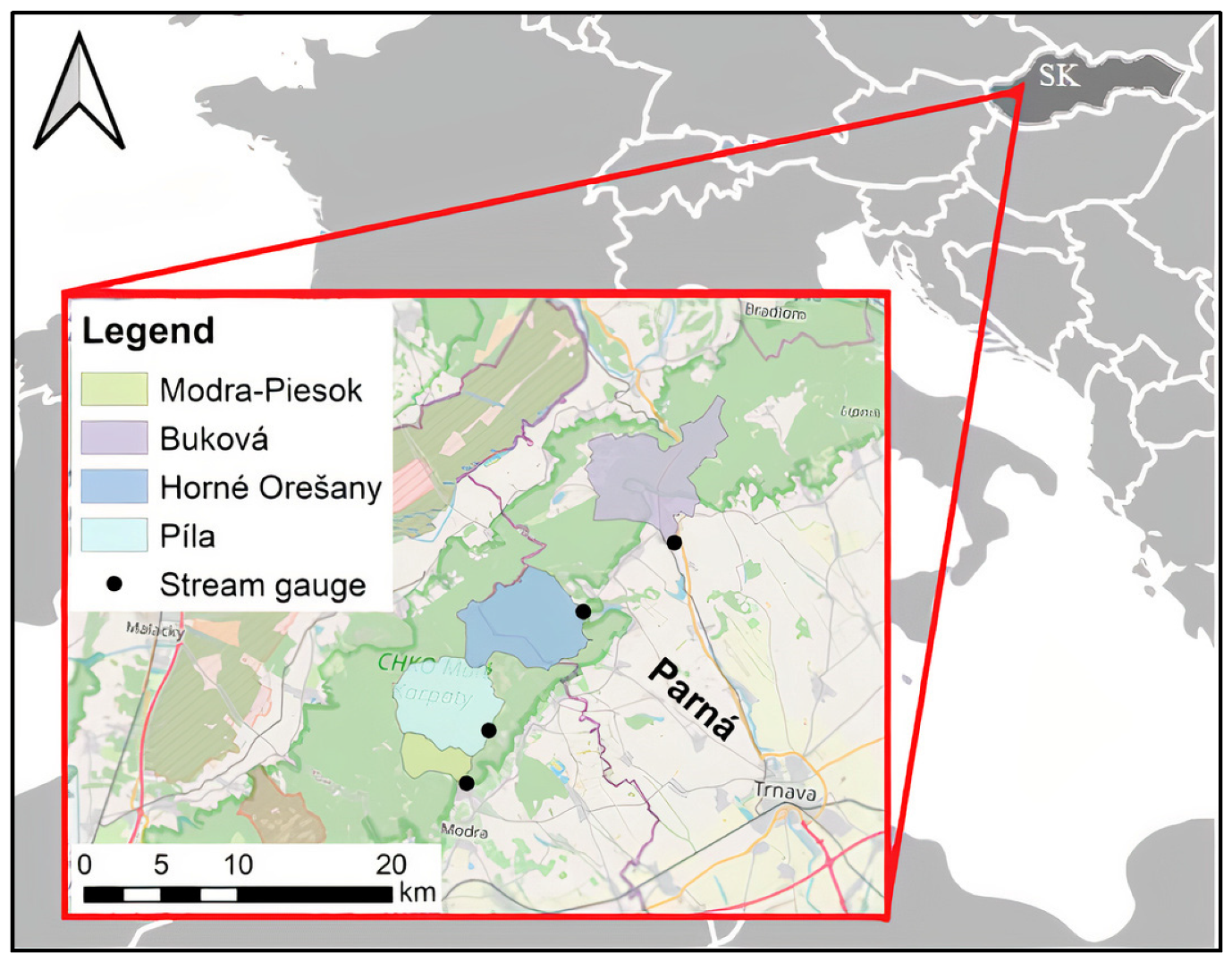
In this case study, a comparison of catchments was tested on four catchments in the Small Carpathians in Western Slovakia (Figure 1); namely, the catchment of the small mountain stream Parná (catchment size—37.33 km2), measured at the Horné Orešany water gauging station, the catchment of the Trnávka stream using the Buková gauging station (42.96 km2), the catchment of the Vištucký stream using the Modra-Piesok station (9.38 km2), and the Gidra stream catchment using the Píla gauging station (32.9 km2). We will henceforth refer to these catchments by the names of their measuring stations.
In a real investigation of catchment similarity aiming to determine the unmeasured flows, the flows in the so-called target catchments are unknown. However, all selected catchments had measured flows in the presented study, meaning that it was possible to evaluate the relationship between their physical and hydrological similarity. To obtain more results, each catchment was alternately considered as unmeasured, and the remaining three catchments were understood as those from which we seek the most similar to this “unmeasured catchment”; so, we de facto examined the mutual similarity of all catchments.
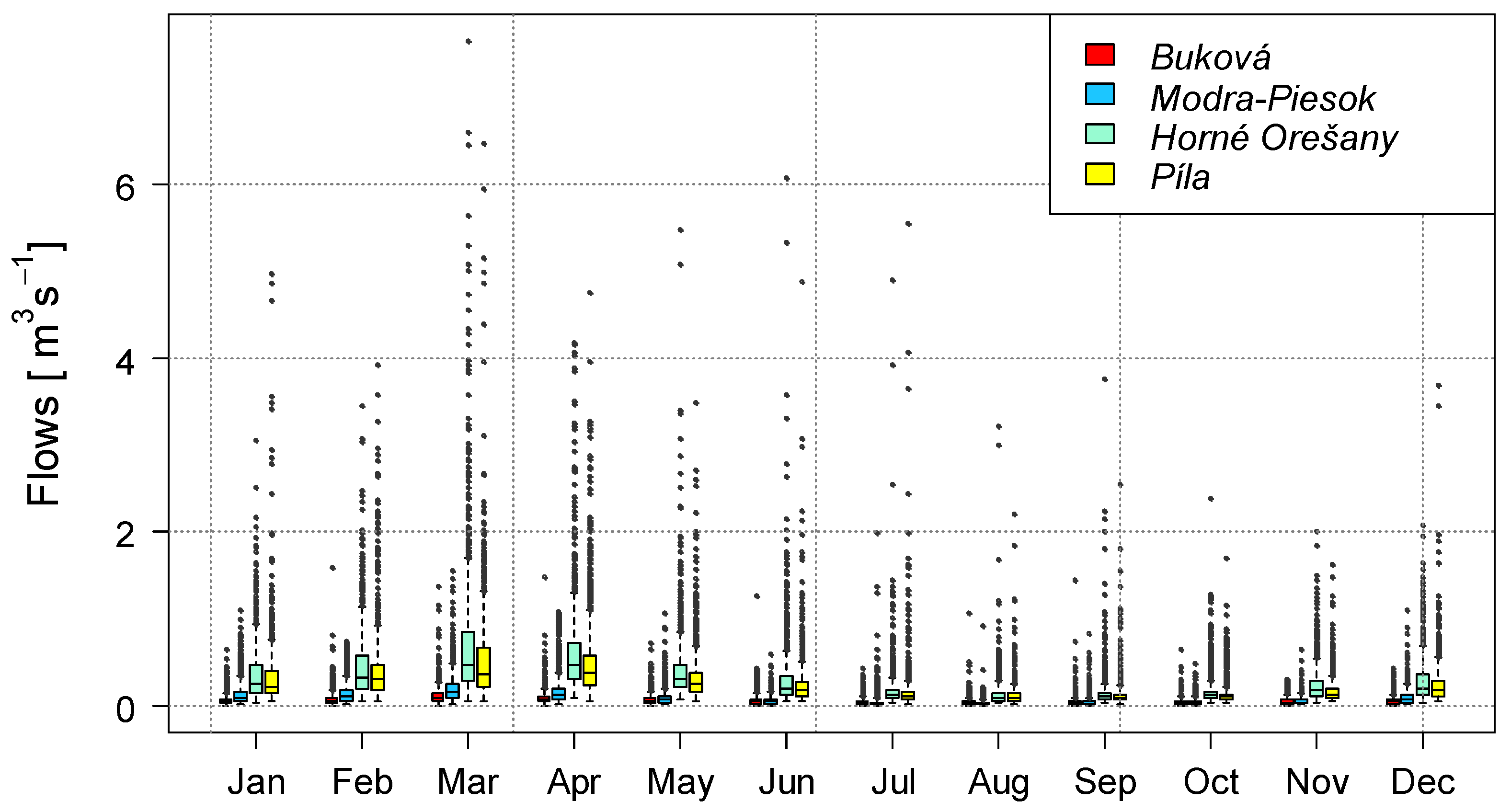
The daily flow data for all the river catchments were obtained from the Slovak Hydro-meteorological Institute in Bratislava, Slovakia for the years 1980 to 2017. These data were used to create a rainfall-runoff models and, at the end of the work, to verify the similarity of the catchments determined based on other characteristics of the catchment. They were not used to determine similarity, as one catchment is always considered unmeasured. The data on precipitation and temperatures were also obtained from the same institution and used in rainfall-runoff modelling, not in determining the similarity of the catchments, as they are nearby areas. The distribution of flow data is shown in Figure 2. The average monthly precipitation totals and temperatures in the area of interest are provided in Table 1.
As neighboring catchments were investigated, it can be assumed that their properties, i.e., climate, topography, geology, soil cover, land use, the genesis of runoff, etc., were similar but not identical. Differences are analyzed in the Results section in such a way that in terms of each catchment descriptor, the least similar catchment to the others is always identified.
3. Methodology
In this work, digital elevation models (DEMs), land use maps, soil maps, and various other information sources were used to analyze the properties of the study area that influence runoff. The characteristics of the catchments investigated are reviewed below.
Various geometric properties influencing a catchment’s hydrological response, including the catchment’s area, perimeter, stream length, catchment length, and various catchment shape factors such as the form factor, circulation ratio, and elongation ratio, were determined using GIS software. The methods for determining these characteristics are well-known and can easily be found in the established hydrological literature [23,24,25]. For this reason, we present the methodology for their determination in Appendix A.
The topographic characteristics were derived from a DEM using GIS software. QGIS [26] and R software [27] were the primary tools used. The topographic similarity was examined using a digital elevation model with a grid size of 20 × 20 m. The characteristics evaluated included altitude, slope, and aspect, among others. Higher altitudes were accompanied by a higher total rainfall, depth, snow cover duration, and reduced temperature. Statistical methods and a hypsometric curve were used to compare the altitudes of the catchments; the hypsometric curve represents the relative area below (or above) a given altitude [28] and describes the distributions of elevations across a catchment. A catchment’s slope determines the direction and speed of the runoff [29].
Both the composition of the bedrock and soil properties also significantly influence the hydrological response of a catchment, as these characteristics result in a different rate of rainfall infiltration, percolation, retention of soil moisture, etc. [29].
The parent rock and terrain also influence the formation of the drainage networks of the catchments, which were evaluated based on their density. A digital elevation model and QGIS software were used for mapping the drainage networks and evaluating their density.
Land cover is another crucial factor; it encompasses the percentage of forest soil, agricultural soil, and the built-up area in the catchment. Runoff is usually slowed by forest cover because it influences hydrological processes such as interception, rainfall infiltration, evaporation, and transpiration. Conversely, a built-up area or improperly cultivated arable land accelerates outflow [30]. The areas of the individual land-use types in the examined localities were compared using GIS tools.
The climatic similarity between catchments can be evaluated by comparing factors such as precipitation, temperature, differences in rainfall, and potential evapotranspiration. Quite often, climate has been identified as the most important driving factor for different hydrological behaviours [5,6]. However, when comparing only nearby catchments, as is the case in this study, the climatic differences are usually negligible. As such, this work devotes minimal space to this factor.
This work also introduces the catchment characteristic “calibrability”, which is the level of precision achieved via the hydrological modelling of flows. Suppose we are investigating the similarity of catchments with the goal of creating a hydrological model for unmeasured catchments. If the flows cannot be modelled with sufficient precision in a measured catchment, transferring the model parameters to another, unmeasured catchment model, would be probably even less successful. The engineers solving the task in which the determination of unknown flows will be used must assess what level of accuracy is still acceptable in a particular task context, i.e., it would be different in the introductory study of an irrigation system design and different in a detailed design of flood protection. In general, however, it can be said that the determination of flow rates below a Nash–Sutcliffe efficiency of 0.5 is insufficient.
In this work, we will therefore use the umbrella term “calibrability” to emphasise the context in which it is used, to stress the importance of evaluating this aspect in searching for a suitable source (analogous) catchment and also because one must decide how to determine this level of accuracy in a particular task. It is necessary to take into account the purpose for which derived flows will be used. In a real-life task, the engineer may choose different indicators for tasks that address low flows and other indicators for solving flood problems. Identifying this characteristic can also be based on graphical methods (for example, the comparison of measured and calculated hydrograms) or on a combination of several indicators. This characteristic is expressed by the Nash–Sutcliffe coefficient in this work [31], since the purpose for which the similarity of the catchments is evaluated is not addressed in it, and it is a frequently used indicator in the hydrological community. As will be shown in the Results section, it served quite well for the given purpose.
Based on the catchment properties (catchment descriptors), this paper offers a practical penalization methodology for identifying the most similar catchments from a few catchments surrounding an ungauged catchment of interest. In this penalization methodology, some space is left to engineering know-how for considering various irregular details. This is both possible and more appropriate due to the smaller number of catchments than in regional studies. Therefore, we proposed testing the process of determining the overall similarity between catchments using a penalization methodology in which a catchment most dissimilar from the other catchments is penalised by one point. The authors think that the determination of the penalty with different values of the penalty coefficient for each characteristic of the catchment exceeds the current know-how in this issue and exceeds the possibilities of a practical study that does not analyse the whole region.
The “hydrological response” view of catchment similarity was verified using specific flows. These are flows in millimetres per time step, i.e., computed from usual units according to the following formula:
where Qm3/s is the flow in m3 ∗ s−1, Qmm/day is the flow in mm × day−1, and a is the catchment area in km2. We chose these units because the investigated catchments have/can have different areas (so that the flows can be compared). These units are also more advantageous in evaluating the hydrological balance, because evapotranspiration and precipitation are also in mm. The correlation of the specific flows was investigated because the catchments in the presented case study have different areas. In this verification process (Figure 2), the proposed manner of penalization and mentioned unified size of the penalty coefficient was verified. Therefore, the similarity between catchments was evaluated from two points of view, one based on the catchment descriptors (which is an evaluation of the physical similarity) and the other based on the similarity of runoff response. Runoff response of two or more catchments is similar, when flows (time series of flows) have good correlation (e.g., above 0.65). A comparison of these two methods of assessing the similarity of catchments served as verification. In this process, it was verified as to whether both the penalty procedure and the assessment of the hydrological response led to the identification of the same catchment as most similar to the ungauged catchment.
Qmm/day = 86.4 × a−1 × Qm3/s,
4. Results and Discussion
This chapter contains catchment similarity assessments from several viewpoints, i.e., according to various characteristics. In the following, the most different catchment from the others in terms of each characteristic is evaluated. This catchment is penalized by one point. Penalization is summarized, and the overall similarity/dissimilarity of the catchments in question is determined at the end of this chapter in Table 6 (firstly, four auxiliary tables follow).
The basic geometric properties of the catchments, including area, perimeter, catchment length, segmentation of the catchment boundary, form factor, circulation ratio, elongation ratio and shape factor, are evaluated and summarized in Table 2. The value of the most different catchment’s characteristic is marked in bold and is underlined. The most different catchment is then penalized with one point; these points are summed at the bottom. The perimeter and length of the catchments are not evaluated as they are used in the calculations of other (evaluated) geometric characteristics. Based on Table 2, it can be concluded that the Buková catchment is the most dissimilar in terms of geometric properties, and it is recorded in Table 6, which summarizes all the properties.
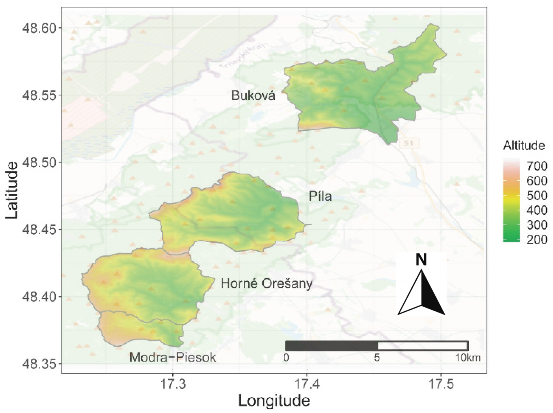
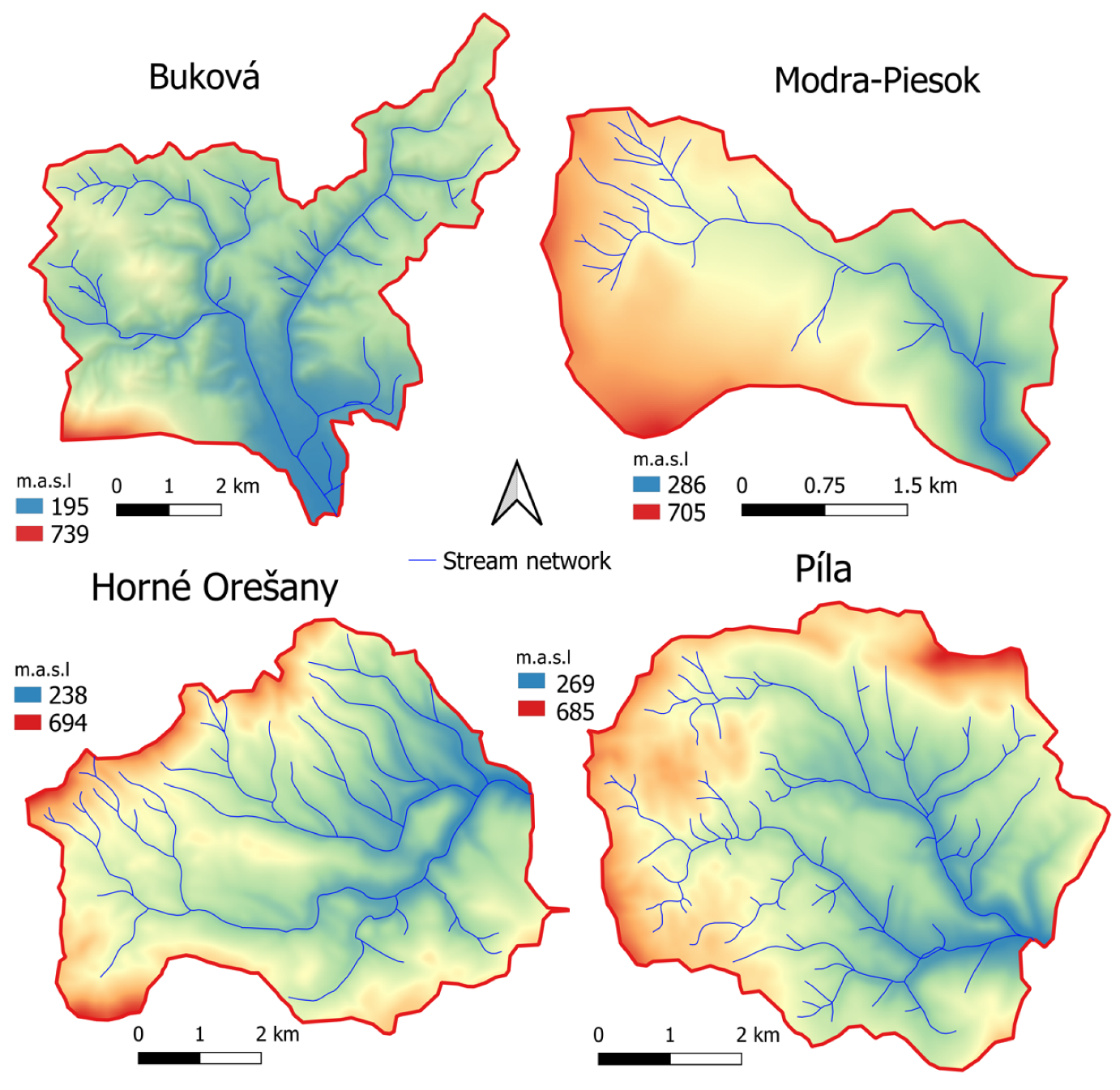
An analysis of the altitude, slope, and orientation of the catchments slopes was performed using a digital elevation model (Figure 3), as these are the primary topographic attributes that influence hydrological processes.
The lowest and highest altitudes were found in the Buková catchment at 195.3 m above sea level and 738.4 m above sea level, respectively (Table 3). Compared to the other catchments, Buková’s median elevation was relatively low, and its elevations also included the highest number of outliers; see Figure 4. Additionally, the Modra-Piesok catchment had the highest median altitude and deviated from the other catchments’ altitude conditions. In terms of this characteristic, Buková and Modra-Piesok are the most different from the other analyzed catchments (and are penalized in Table 6).
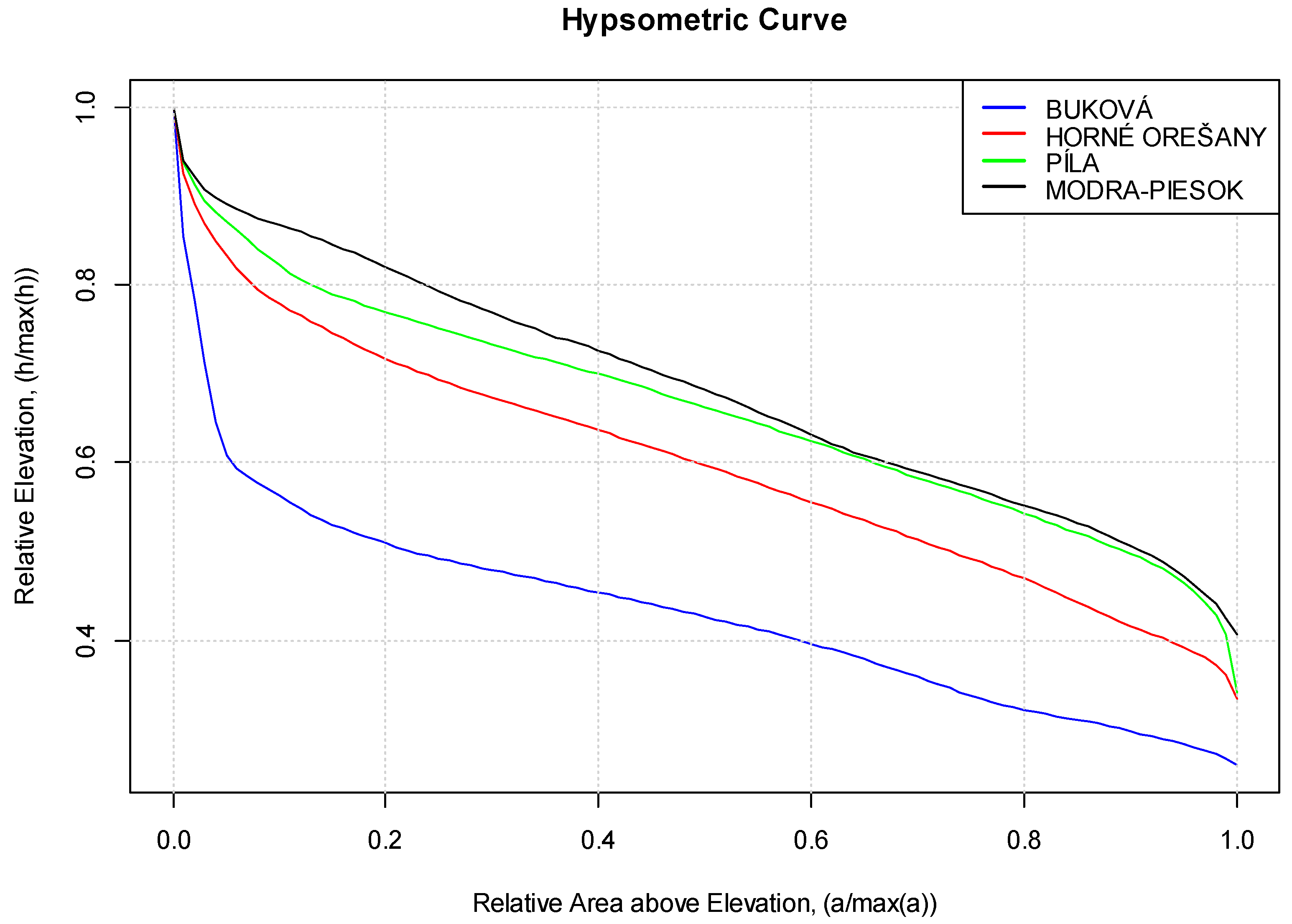
The hypsometric curves of the evaluated catchments are shown in Figure 5, a non-dimensional measure of the proportion of the catchment above a given elevation. Hypsometry is used as an indicator of the geomorphic form of catchments. Many researchers have postulated that this is an important characteristic of a catchment’s form and is useful for explaining various hydrological or erosion processes [24,32]. It is clear from Figure 5 that the hypsometric curve of the Buková catchment differs the most from the other evaluated catchments (penalized in Table 6).
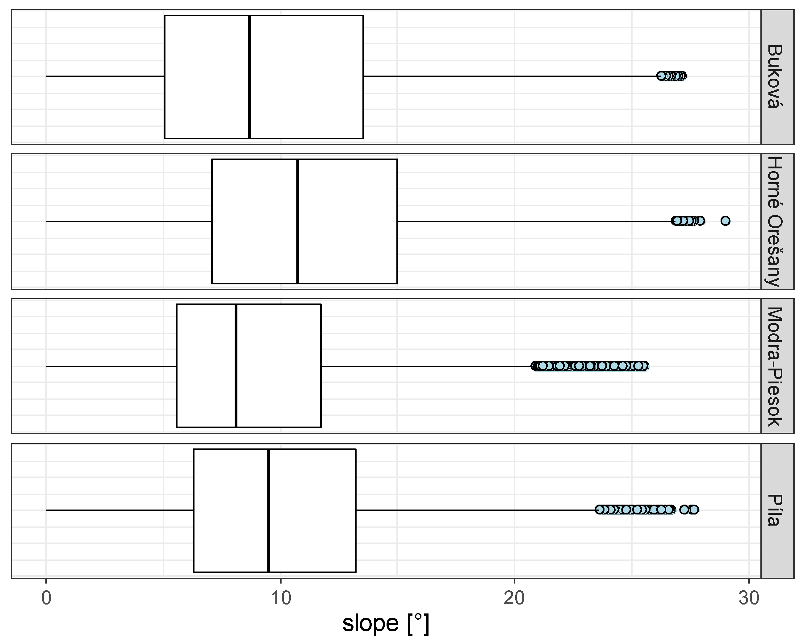
The boxplots of the slopes (Figure 6) show a similar distribution of values in the Buková, Horné Orešany and Píla catchments; the most frequent slope has a value of around 9°. The Modra-Piesok catchment distribution of slope values shows the smallest standard deviation in the set, i.e., 4.46, and the highest skewness (Table 3), so it was evaluated as the most dissimilar to the rest of the evaluated catchments from this point of view (and it is penalized in Table 6).
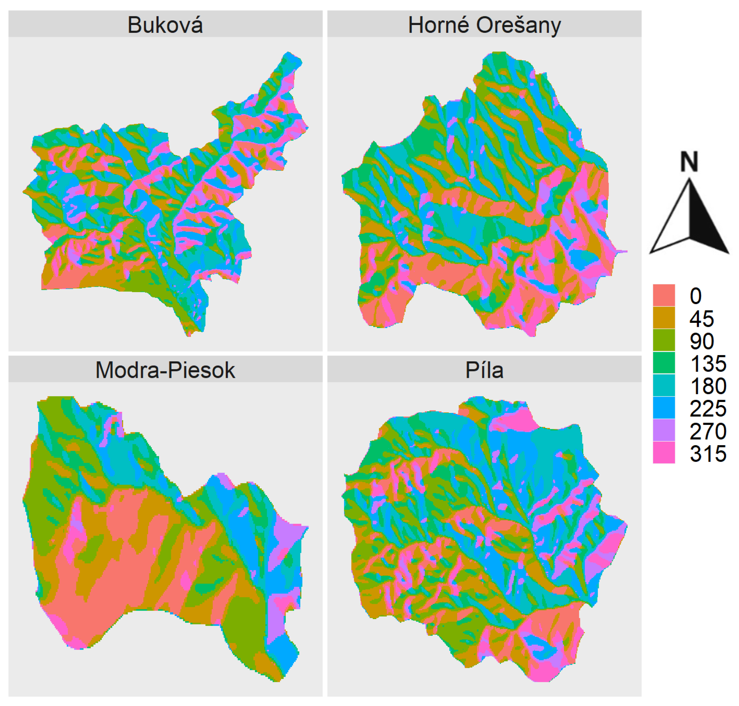
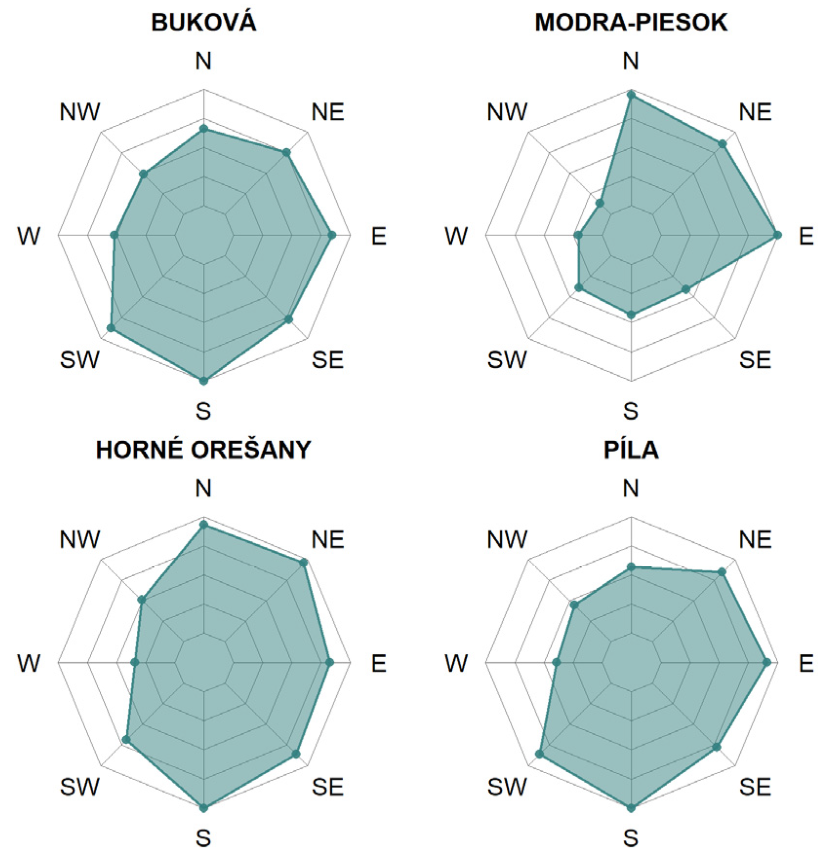
The catchments’ slope aspects, which were obtained through a analysis of their DEMs, are shown in Figure 7 and Figure 8. The working procedures and methodology of these analyses can be found in geoinformatics literature such as the work of Lovelace et al. [33]. Figure 8 shows the so-called radar graph, which summarizes the data on the slope aspect of each catchment. The relative number of cells with a given slope is plotted on each cardinal and intercardinal direction and labelled on the edge of the radar graph. North corresponds to the values of 0° (or 360°), east corresponds to 90°, south to 180°, and west to 270°. Using a relative view enables the comparison of aspects of catchments with different areas. Both the radar plots and the summary in Table 3 led to the overall conclusion that the Modra-Piesok catchment is the most dissimilar in terms of slope aspect.
Table 3 includes a summary of the statistical characteristics of the preceding analyses of the catchments’ altitudes, gradients, and aspects of catchments.
Figure 9 shows the catchments’ drainage network, which was obtained using GIS tools (details are in Appendix A). An important parameter in terms of the outflow regime is the density of the drainage network, which was 1.15 for the Buková catchment; and higher in others, i.e., 1.45, 1.53, and 1.71 for Modra-Piesok, Horné Orešany, and Píla, respectively. The Buková catchment can therefore be considered the most different in terms of drainage network.
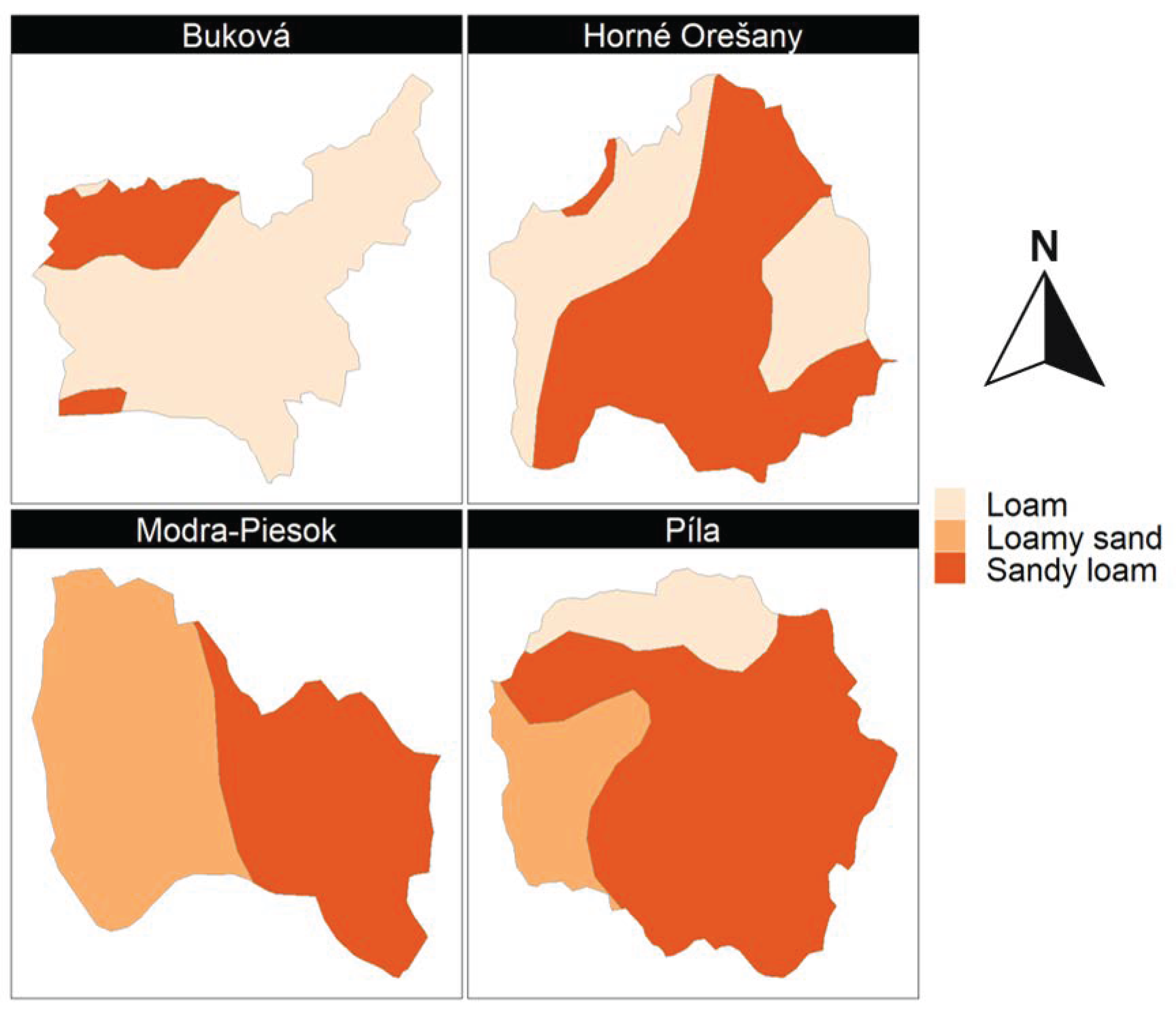
The soils of the catchments investigated consisted exclusively of the loam, sandy loam, and loamy-sand soil textural classes. According to Figure 10, Buková is almost entirely covered by loamy soil, which is less leaky than sandy soils, making it the most dissimilar catchment compared to the other catchments analyzed.
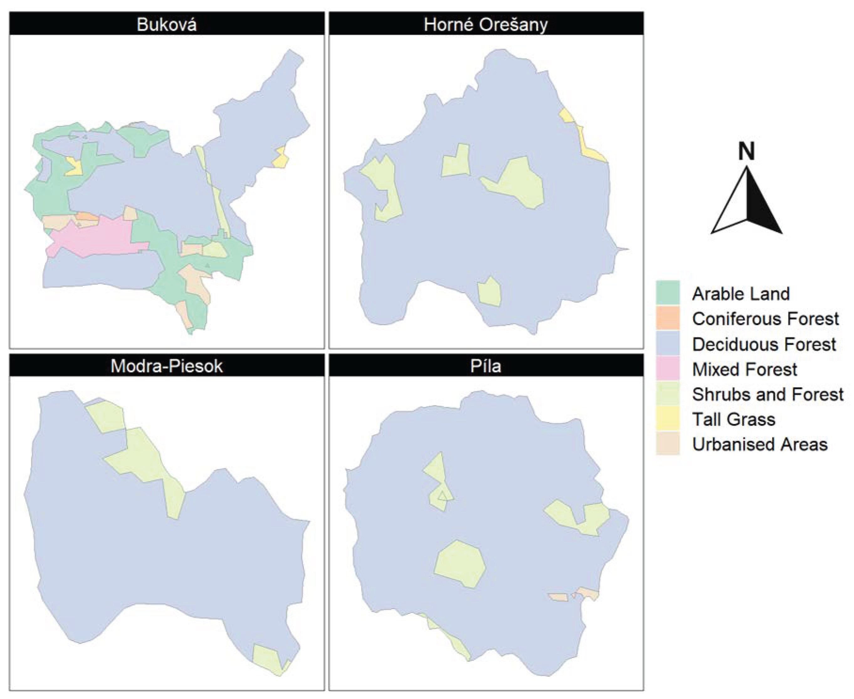
The land use was evaluated in GIS software using a vectorized map. Deciduous forest was the most common type of land cover. Figure 11 shows the high similarity of Horné Orešany, Modra-Piesok, and Píla, which are predominantly covered with deciduous forest and some transition shrubs, i.e., with a land cover that slows down runoff. The Buková catchment is the only one with larger areas of other kinds of land use, mainly arable land and urbanized areas. This catchment also has the least amount of deciduous forest. Arable land and urbanized areas are more susceptible to surface runoff, which significantly influences the hydrological response of the catchment. In sum, Buková is considered the most different catchment; the percentages of the different types of land are shown in Table 4. As with the other catchment characteristics, this assessment is marked by a penalty in Table 6.
4.1. Calibrability
The similarity of catchments was analyzed in this work as a preliminary step toward utilizing this factor in various analyses, such as analogous calculations of river flows in unmeasured catchments. A similar measured (donor) catchment to an unmeasured (target) catchment is sought in such calculations. Then, using the donor catchment, one can calibrate a hydrological model and subsequently use it for a target river catchment.
One important indicator of the suitability of a donor catchment is the possibility to satisfactorily accomplish its rainfall-runoff model’s calibration. We refer to this donor catchment property as “calibrability”. If calibrating the catchment’s model satisfactorily is impossible, then the catchment is not a suitable donor, as its model cannot act as a realistic predictor of flows for another catchment.
Calibrating a hydrological rainfall-runoff model means finding its parameters and ensuring the closest possible agreement of the calculated and measured flows on a given stream. Therefore, on the donor catchment, measured flows are required data to accomplish calibration. “Calibrability” was determined in this work using the TUW hydrological model [34]. This model runs with a daily time step and consists of a snow routine, a soil moisture routine, and a flow routing routine; a genetic algorithm was used to calibrate its 15 parameters. The level of precision of the final model (agreement between measured and computed flows) for all catchments, as expressed by the value of the Nash–Sutcliffe (NSE) coefficient, is shown in Table 5.
The highest “calibrability” (NSE values of 0.681 and 0.683) was evaluated for the Píla and Modra-Piesok catchments. They are, therefore, suitable candidates for use as donor catchments. The lowest “calibrability” value was seen in the Buková catchment (0.426); an NSE value lower than 0.5 cannot be accepted as satisfactory. Therefore, it can be concluded that the Buková catchment is not appropriate for the hydrological analogy and is also penalized in Table 6 from this point of view.
4.2. Overall Assessment of the Similarity of the Catchments
The overall evaluation of the similarity of the catchments was undertaken using penalization. As previously mentioned, this method is more appropriate for a task in which (for engineering purposes) a smaller number of catchments are analyzed, as opposed to a task in which the whole region is analyzed. It is clear from the literature review that a smaller number of works in the hydrological literature have been dedicated to this practical task. For each previously discussed characteristic, the most dissimilar catchment from the others scored one point, as shown in Table 6. In some ambiguous cases, the second least similar catchment was also given a point if it was also significantly different from the others. The penalization results of the individual catchments, together with their overall total, are shown in Table 6.
Horné Orešany, and Píla were not penalized in any category, and the most often penalized (and thus most different) catchment was Buková, with eight points. The climate indicators are not listed in Table 6, as a high similarity level was reported in terms of the climate conditions across all examined catchments.
In a real-life setting, determining the flows of a target catchment would involve one catchment with unknown flows (target) and the evaluation of the best possible choice (the most similar catchment) from potential donor catchments. In Table 6, the best choice of donor catchment when each catchment is considered the target is evaluated.
For the Horné Orešany catchment, the best donor catchment is Píla; the second-best option is Modra-Piesok (Table 7). The situation is similar when Píla is the target catchment, and Modra-Piesok could also use Píla and Horné Orešany as donor catchments. It would be most appropriate to look for other donor catchments for Buková, the least similar to all the other evaluated catchments.
4.3. Verification of Similarity Using Specific Flows
The purpose of this subchapter is to verify the proposed assessment of the similarity of catchments based on their hydrological response.
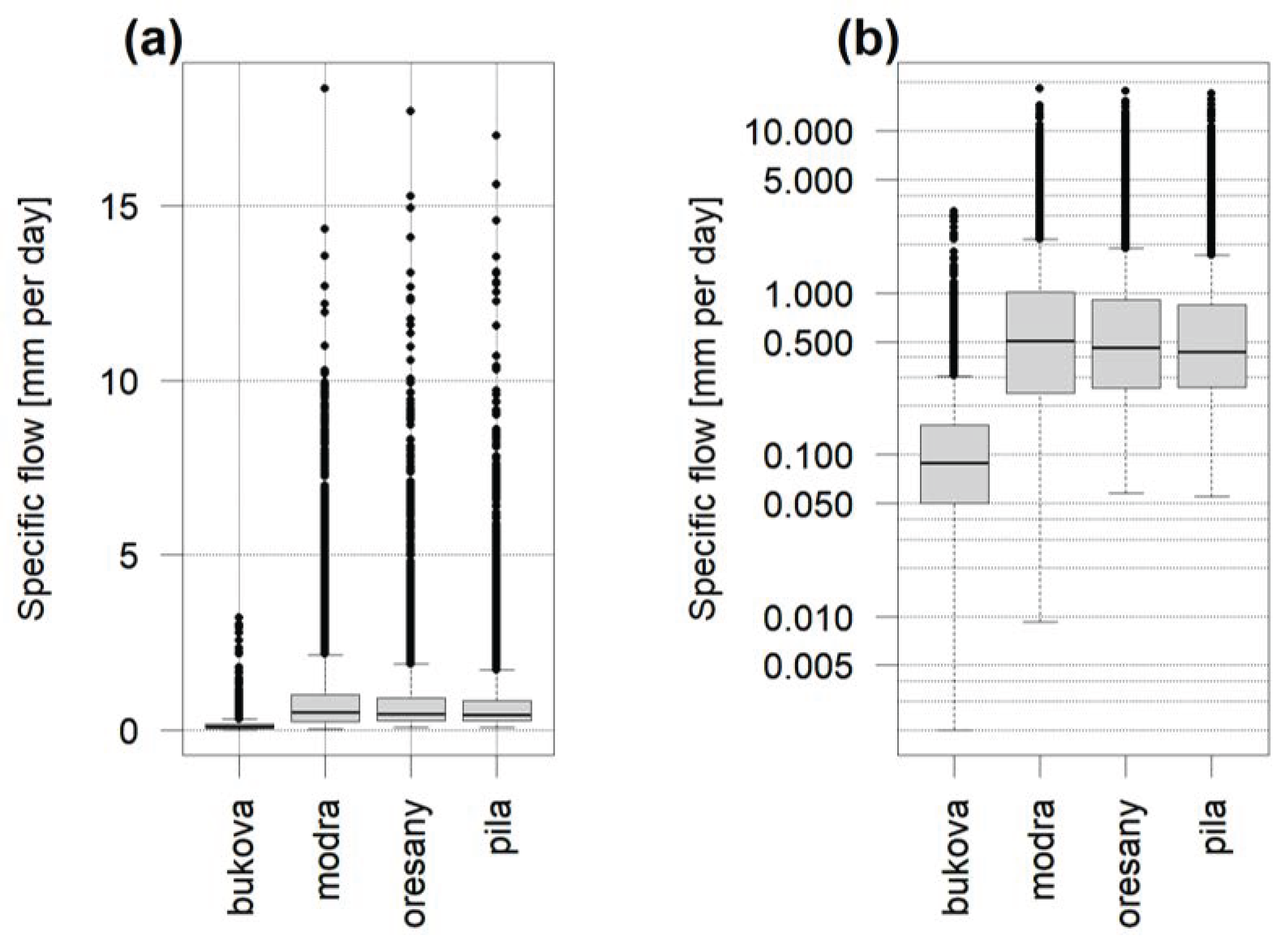
Catchments with known flows were selected to test the above-described evaluation of the similarity. We did not directly compare flows in the riverbed, but specific flows, as the catchments vary in size. The specific flows are flows per unit area of the catchment (in mm) and are compared in Figure 12a using box plots. Figure 12b shows the same flows, but their logarithms are displayed for clarity, making the similarity/dissimilarity between the catchments more evident. The smallest specific flows are in the Buková catchment; this finding confirms our methodology of examining the physical similarity of the catchments. From that viewpoint, the Buková catchment was also the least similar to other catchments. The flows of the other catchments are quite similar (as can be seen in Figure 12b; they have close values of their medians, quartiles and outliers).
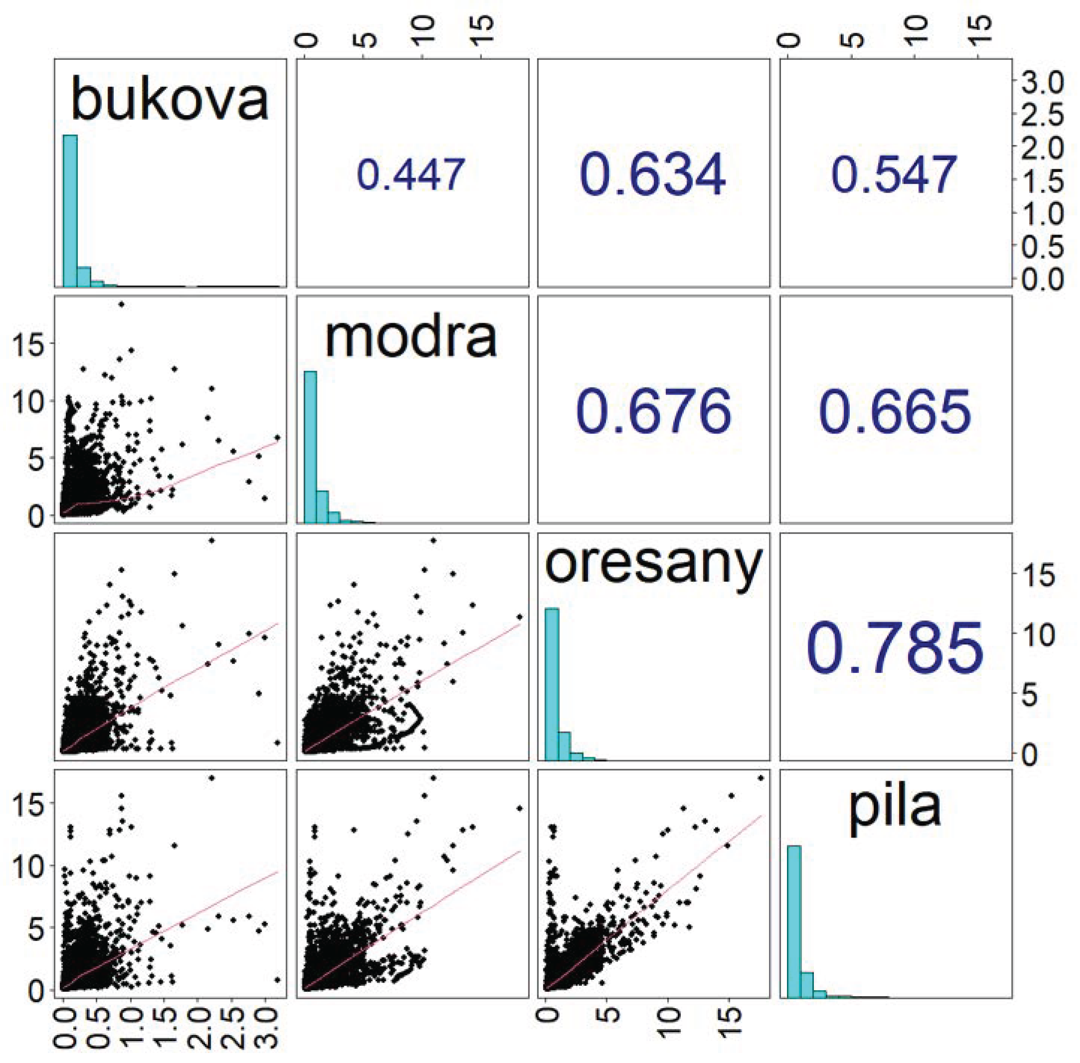
The proposed method of catchment similarity assessment was also verified using flow correlations. The mutual relation between specific flows is expressed in Figure 13 through a plot of the correlation matrix. This matrix makes it possible to see which catchments have the most similar hydrological regimes to others and which are different. A correlation plot shows in the cells above the diagonal the correlation coefficients between the variables (time series of flows), which are identified by the gauging station name on the diagonal of the matrix. The correlation coefficient in a particular cell is between those two variables, which are in the vertical and horizontal directions from the diagonal. This figure serves as a quick overview of the flow data; therefore, mini histograms and mini scatter plots of all pairs of variables (flows) are also presented. The assignment of the variables for these mini plots is similar to in the case of the correlation coefficients. The average correlation coefficient could be easily evaluated for each catchment; it could be used to characterize a given catchment’s overall similarity/dissimilarity to others. This average is the smallest for the Buková catchment (0.54), again confirming its dissimilarity. Such catchments should not be used for calculating flows for unmeasured catchments. The low correlation can mean that there are factors in the catchment that influence its runoff that are not present in the other catchments or the given area. Average correlation coefficients with other catchments are as follows: for Horné Orešany, 0.66, Modra-Piesok, 0.60, Buková, 0.54, and Píla, 0.67. The scatterplots under a diagonal in Figure 13 graphically illustrate the similarity/dissimilarity of the catchments; the smaller the dispersion of points around the regression line, the more hydrologically similar a given pair of catchments are.
5. Conclusions
This case study evaluated the similarity of the catchments in terms of several factors that influence the rainfall-runoff process. Properties such as slopes, altitudes, soils, land use, and “calibrability” help to determine a catchment’s similarity in this work. The similarity identified has potential applications in various engineering tasks, e.g., it is useful for determining flows in unmeasured catchments. The overall similarity was evaluated using the proposed penalty method. The proposed method and results obtained were preliminarily verified using the flows from the catchments to detect whether physically similar/dissimilar catchments are also hydraulically similar/dissimilar. The results confirm this hypothesis, and also confirm the correctness of the proposed penalty procedure, meaning that this study’s results can, after further extensive testing, be used in practical water engineering tasks.
The authors are aware that the problem in question is a very complex and not yet fully explored area of research. However, even at the current, still open level of research, similar problems need to be addressed in practice. This case study should contribute to a practical solution and does not have the aim of solving complex theoretical issues related to the similarity of catchments and the calculation of flows in unmeasured catchments. For this reason, the authors are considering the further verification of this method for larger areas and using the proposed methodology of identifying the similarity of catchments for engineering tasks in their subsequent works.
Author Contributions
Conceptualization, M.C.; methodology, M.C.; software, B.P.; data curation, B.P. and M.A.; writing—original draft preparation, M.C. and B.P.; writing—review and editing, B.P.; visualization, M.A.; Funding acquisition, M.C. All authors have read and agreed to the published version of the manuscript.
Funding
This research was funded by the Slovak Research and Development Agency under Contract No. APVV-19-0383 “Natural and technical measures oriented to water retention in sub-mountain watersheds of Slovakia” and by the Scientific Grant Agency of the Ministry of Education of the Slovak Republic and the Slovak Academy of Sciences, Grant No. 1/0662/19.
Institutional Review Board Statement
Not applicable.
Informed Consent Statement
Not applicable.
Data Availability Statement
The data presented in this study are partly available on request from the corresponding author. Some of the data are only available from the Slovak Hydro-meteorological Institute in Bratislava on a commercial basis.
Acknowledgments
This work was supported by the Slovak Research and Development Agency under Contract No. APVV-19-0383 “Natural and technical measures oriented to water retention in sub-mountain watersheds of Slovakia” and by the Scientific Grant Agency of the Ministry of Education of the Slovak Republic and the Slovak Academy of Sciences.
Conflicts of Interest
The authors declare no conflict of interest.
Appendix A
This appendix provides details of some methodological procedures.
Appendix A.1. Determination of Geometric Characteristics
Appendix A.1.1. Catchment Area (A), Catchment Perimeter (P) and Stream Length (Ls)
The basic geometric characteristics were determined in QGIS [25] software based on the digital map work SVM 50, which was created on the basis of the basic map of the Slovak Republic at a scale of 1:50,000 (ZM50). Thematic maps of watercourses and other water bodies, catchments and DEM were used in this work. The S-JTSK coordinate system is used in these maps.
Appendix A.1.2. Catchment Length (LC)
Catchment length is somewhat ambiguously defined in the hydrological literature [35] and can be defined in more than one way—it can be the longest straight line distance between any two points on the perimeter or the greatest distance between the outlet and any point on the perimeter or the length of the main stream from its source (projected to the perimeter) to the outlet, etc. In this work was length of catchment defined as the length of the simplified main stream from its source (projected to the perimeter) to the outlet.
Figure A1.
Illustration of catchment length determination.

Form factor [22]
The area of the catchment divided by the square of length of the catchment:
Ff = A/LC
- A
- Catchment area [km2]
- LC
- Catchment length [km]
Circulation ratio [24]
Rc = A/Ac
- Ac
- the area of a circle having equal perimeter as the perimeter of drainage catchment in [km2]
Elongation ratio [36]
Re = 2 × LC × A0.5/π
Shape factor [22]
Catchment boundary segmentation
CBS = P/(2 × (π × A)0.5)
Appendix A.2. The Drainage Network Creation
Since the authors of the article had at their disposal the mentioned digital maps SVM 50, including a map of watercourses, this map was used to determine the length of the river network. Using QGIS commands, the total length of the river network was identified. The basic QGIS commands were also used to identify catchments areas. By dividing the length of the river network by the catchment area, the density of the river network is evaluated. If it is necessary to determine the drainage network, it can be generated from a digital terrain model. E.g., SAGA GIS commands integrated into QGIS could be used, specifically the “Channel network” module. This module requires a grid that contains elevation data and various parameters such as the minimum segment length and different algorithm initiation parameters. The output of the command is a grid and vector version of the drainage network.
Appendix A.3. Hydrologic Modelling in Context of the “Calibrability” Evaluation
The flows in every catchment were calculated in R software ecosystem by the TUW conceptual rainfall-runoff model [33], with a genetic algorithm used for calibration [37]. The calibration was implemented based on flow and climate data from time period 1980–2005. The remaining available data for the years 2006 to 2017 were used to evaluate the calibrated model. The results of this testing were used to calculate the flows, which were used to determine the NSE statistics in Table 5. The genetic algorithm population was set to 500, the number of parameters to be determined was 15, and the maximum number of generations was set to 20. The objective function sought to maximize the NSE.
References
- Blöschl, G.; Sivapalan, M.; Wagener, T.; Savenije, H.; Viglione, A. (Eds.) Runoff Prediction in Ungauged Basins, Synthesis Across Processes, Places and Scales; Cambridge University Press: Cambridge, UK, 2013. [Google Scholar]
- Wagener, T.; Sivapalan, M.; Troch, P.; Woods, R. Catchment classication and hydrologic similarity. Geogr. Compass 2007, 1, 901–931. [Google Scholar] [CrossRef]
- Teutschbein, C.; Grabs, T.; Laudon, H.; Karlsen, R.H.; Bishop, K. Simulating streamflow in ungauged basins under a changing climate: The importance of landscape characteristics. J. Hydrol. 2018, 561, 160–178. [Google Scholar] [CrossRef]
- Jehn, F.U.; Bestian, K.; Breuer, L.; Kraft, P.; Houska, T. Using hydrological and climatic catchment clusters to explore drivers of catchment behavior. Hydrol. Earth Syst. Sci. 2020, 24, 1081–1100. [Google Scholar] [CrossRef] [Green Version]
- Sawicz, K.; Wagener, T.; Sivapalan, M.; Troch, P.A.; Carrillo, G. Catchment classification: Empirical analysis of hydrologic similarity based on catchment function in the Eastern USA. Hydrol. Earth Syst. Sci. 2011, 15, 2895–2911. [Google Scholar] [CrossRef] [Green Version]
- Kuentz, A.; Arheimer, B.; Hundecha, Y.; Wagener, T. Understanding hydrologic variability across Europe through catchment classification. Hydrol. Earth Syst. Sci. 2017, 21, 2863–2879. [Google Scholar] [CrossRef] [Green Version]
- Oudin, L.; Andréassian, V.; Perrin, C.; Michel, C.; Le Moine, N. Spatial proximity, physical similarity, regression and ungaged catchments: A comparison of regionalization approaches based on 913 French catchments. Water Resour. Res. 2008, 44, W03413. [Google Scholar] [CrossRef]
- Loritz, R.; Gupta, H.; Jackisch, C.; Westhoff, M.; Kleidon, A.; Ehret, U.; Zehe, E. On the dynamic nature of hydrological similarity. Hydrol. Earth Syst. Sci. 2018, 22, 3663–3684. [Google Scholar] [CrossRef] [Green Version]
- Xiao, D.; Shi, Y.; Brantley, S.L.; Forsythe, B.; DiBiase, R.; Davis, K.; Li, L. Streamflow generation from catchments of contrasting lithologies: The role of soil properties, topography, and catchment size. Water Resour. Res. 2019, 55, 9234–9257. [Google Scholar] [CrossRef] [Green Version]
- Blöschl, G.; Sivapalan, M. Scale issues in hydrological modelling: A review. Hydrol. Process. 1995, 9, 251–290. [Google Scholar] [CrossRef]
- Hrachowitz, M.; Savenije, H.H.G.; Blöschl, G.; McDonnell, J.J.; Sivapalan, M.; Pomeroy, J.W.; Arheimer, B.; Blume, T.; Clark, M.P.; Ehret, U.; et al. A decade of predictions in ungauged basins (PUB)—A review. Hydrol. Sci. J. 2013, 58, 1198–1255. [Google Scholar] [CrossRef]
- Guo, Y.; Zhang, Y.; Zhang, L.; Wang, Z. Regionalization of hydrological modeling for predicting streamflow in ungauged catchments: A comprehensive review. WIREs Water 2021, 8, e1487. [Google Scholar] [CrossRef]
- Parajka, J.; Merz, R.; Blöschl, G. A comparison of regionalisation methods for catchment model parameters. Hydrol. Earth Syst. Sci. 2005, 9, 157–171. [Google Scholar] [CrossRef] [Green Version]
- Zhang, Y.; Chiew, F.H. Relative merits of different methods for runoff predictions in ungauged catchments. Water Resour. Res. 2009, 45. [Google Scholar] [CrossRef]
- Zhao, Q.; Zhu, Y.; Wan, D.; Yu, Y.; Lu, Y. Similarity analysis of small-and medium-sized watersheds based on clustering ensemble model. Water 2020, 12, 69. [Google Scholar] [CrossRef] [Green Version]
- Rao, A.R.; Srinivas, V.V. Regionalization of watersheds by hybrid-cluster analysis. J. Hydrol. 2006, 318, 37–56. [Google Scholar] [CrossRef]
- Narbondo, S.; Gorgoglione, A.; Crisci, M.; Chreties, C. Enhancing physical similarity approach to predict runoff in ungauged watersheds in sub-tropical regions. Water 2020, 12, 528. [Google Scholar] [CrossRef] [Green Version]
- Aytaç, E. Unsupervised learning approach in dening the similarity of catchments: Hydrological response unit based k-means clustering, a demonstration on Western Black Sea Region of Turkey. Int. Soil Water Conserv. Res. 2020, 8, 321–331. [Google Scholar] [CrossRef]
- Bhatta, B.; Shrestha, S.; Shrestha, P.K.; Talchabhadel, R. Evaluation and application of a SWAT model to assess the climate change impact on the hydrology of the Himalayan River Basin. Catena 2019, 181, 104082. [Google Scholar] [CrossRef]
- Samaniego, L.; Bárdossy, A.; Kumar, R. Streamflow prediction in ungauged catchments using copula-based dissimilarity measures. Water Resour. Res. 2010, 46, 46. [Google Scholar] [CrossRef]
- Kohonen, T. Self-Organizing Maps; Springer: Berlin, Germany, 2001. [Google Scholar]
- Wallner, M.; Haberlandt, U.; Dietrich, J. A one-step similarity approach for the regionalization of hydrological model parameters based on Self-Organizing Maps. J. Hydrol. 2013, 494, 59–71. [Google Scholar] [CrossRef]
- Horton, R.E. Erosional development of streams and their drainage basins; Hydrophysical approach to quantitative morphology. Bull. Geol. Soc. Am. 1945, 56, 275–370. [Google Scholar] [CrossRef] [Green Version]
- Strahler, A.N. Quantitative geomorphology of drainage basin and channel networks. In Handbook of Applied Hydrology; Chow, V.T., Ed.; McGraw Hill: New York, NY, USA, 1964. [Google Scholar]
- Miller, V.C. A Quantitative Geomorphic Study of Drainage Basin Characteristics in the Clinch Mountain Area. Virginia and Tennessee; Technical Report 3; Office of Naval Research, Department of Geology, Geography Branch, Columbia University: New York, NY, USA, 1953. [Google Scholar]
- QGIS Development Team. QGIS Geographic Information System; Open-Source Geospatial Foundation: Beaverton, OR, USA, 2009; Available online: http://qgis.org (accessed on 13 October 2021).
- R Core Team. R: A Language and Environment for Statistical Computing; R Foundation for Statistical Computing: Vienna, Austria, 2020; Available online: https://www.R-project.org/ (accessed on 13 October 2021).
- Strahler, A.N. Hypsometric (area-altitude) analysis of erosional topology. Geol. Soc. Am. Bull. 1952, 63, 1117–1142. [Google Scholar] [CrossRef]
- Mohamoud, Y. Comparison of Hydrologic Responses at Different Watershed Scales; Office of Research and Development, United States Environmental Protection Agency: Research Triangle Park, NC, USA, 2004.
- Zheng, Q.; Hao, L.; Huang, X.; Sun, L.; Sun, G. Effects of urbanization on watershed evapotranspiration and its components in southern China. Water 2020, 12, 645. [Google Scholar] [CrossRef] [Green Version]
- Nash, J.E.; Sutcliffe, J.V. River flow forecasting through conceptual models part I—A discussion of principles. J. Hydrol. 1970, 10, 282–290. [Google Scholar] [CrossRef]
- Schumm, S.A.; Mosley, M.P.; Weaver, W.E. Experimental Fluvial Geomorphology; Wiley: New York, NY, USA, 1987. [Google Scholar]
- Lovelace, R.; Nowosad, J.; Muenchow, J. Geocomputation with R; CRC Press: Boca Raton, FL, USA, 2019. [Google Scholar]
- Viglione, A.; Parajka, J. TUWmodel: Lumped Hydrological Model for Education Purposes. R Package Version 1.0–1. 2018. Available online: https://CRAN.R-project.org/package=TUWmodel (accessed on 13 October 2021).
- Zavoianu, I. Morphometry of Drainage Basins; Elsevier: Amsterdam, The Netherlands, 2011. [Google Scholar]
- Schumm, S.A. Evolution of drainage systems and slopes in badlands at Perth Amboy, New Jersey. Geol. Soc. Am. Bull. 1956, 67, 597–646. [Google Scholar] [CrossRef]
- Walter, R.M., Jr.; Sekhon, J.S. Genetic optimization using derivatives: The rgenoud package for R. J. Stat. Softw. 2011, 42, 1–26. Available online: http://www.jstatsoft.org/v42/i11/ (accessed on 13 October 2021).
Figure 1.
Location of selected catchments.

Figure 2.
Distribution of flows during the year.

Figure 3.
Digital elevation models used for the analyses of the catchments.

Figure 4.
Distribution of altitudes, evaluated by boxplots.

Figure 5.
The hypsometric curves of the evaluated catchments.

Figure 6.
Distribution of slopes, evaluated by boxplots.

Figure 7.
GIS analysis of the slope aspect of the catchments under consideration.

Figure 8.
Radar plots for the summarization of the aspect of the catchment slopes.

Figure 9.
Drainage network of the catchments.

Figure 10.
Maps of soil textural classes in catchments.

Figure 11.
Land use in the catchments under consideration.

Figure 12.
Box plots of the specific flows (in mm/day). (a) y-axis has normal scale, (b) y-axis has logarithmic scale.
Figure 12.
Box plots of the specific flows (in mm/day). (a) y-axis has normal scale, (b) y-axis has logarithmic scale.

Figure 13.
Correlation matrix of the specific flows of the catchments under consideration.


Table 1.
The basic climatic characteristics of the area investigated.
| Characteristics | Month | |||||||||||
|---|---|---|---|---|---|---|---|---|---|---|---|---|
| 1 | 2 | 3 | 4 | 5 | 6 | 7 | 8 | 9 | 10 | 11 | 12 | |
| Monthly totals of precipitation (mm) | 37 | 37.1 | 37.7 | 38.1 | 62.2 | 66.6 | 65.3 | 62.2 | 57 | 42.9 | 47.3 | 43.3 |
| Average monthly temperature (°C) | −0.9 | 0.7 | 4.9 | 9.9 | 14.8 | 17.9 | 20 | 19.4 | 14.8 | 9.6 | 4.4 | 0.3 |
Table 2.
The basic geometric properties of the catchments.
| Characteristic | Catchment | |||
|---|---|---|---|---|
| Buková | Modra-Piesok | Horné Orešany | Píla | |
| area [km2] | 42.96 * | 9.38 | 37.33 | 32.90 |
| perimeter [km] | 39.65 | 15 | 29 | 24.55 |
| catchment length [m] | 10950 | 5740 | 8764 | 7326 |
| catchment boundary segmentation | 1.71 | 1.38 | 1.34 | 1.21 |
| form factor | 0.36 | 0.28 | 0.49 | 0.61 |
| circular ratio | 0.34 | 0.52 | 0.56 | 0.69 |
| elongation ratio | 0.38 | 0.34 | 0.44 | 0.5 |
| shape factor | 2.79 | 3.51 | 2.06 | 1.63 |
| Sum of geometric penalties | 3 | 2 | 0 | 1 |
* Bold and underlined font indicates the most different value for the given characteristic.
Table 3.
Statistical characteristics describing the catchments’ topographical features.
| Characteristic | Catchment | ||||
|---|---|---|---|---|---|
| Horné Orešany | Píla | Buková | Modra-Piesok | ||
| Altitude | max | 693.65 | 684.92 | 738.35 | 704.64 |
| min | 238.26 | 269.05 | 195.31 | 286.94 | |
| mean | 406.97 | 434.25 | 332.47 | 488.21 | |
| sd | 82.41 | 79.50 | 72.40 | 85.94 | |
| skewness | 0.44 | 0.34 | 0.91 | −0.13 | |
| Slope | max | 29.02 | 27.66 | 27.17 | 25.55 |
| mean | 11.12 | 9.91 | 9.47 | 8.92 | |
| sd | 5.25 | 4.76 | 5.71 | 4.46 | |
| skewness | 0.22 | 0.31 | 0.46 | 0.72 | |
| Aspect | mean | 134.23 | 145.61 | 149.56 | 102.18 |
| sd | 96.16 | 91.79 | 94.55 | 87.72 | |
| skewness | 0.27 | 0.14 | 0.05 | 0.69 | |
Table 4.
Percentage of areas of land use in the catchments under consideration.
| Characteristics | Catchment | ||||
|---|---|---|---|---|---|
| Horné Orešany | Píla | Buková | Modra-Piesok | ||
| Land use | Deciduous forest | 88.91 | 91.17 | 51.17 | 89.13 |
| Arable land | - | - | 20.24 | - | |
| Bushy or herbaceous vegetation with scattered trees | 9.25 | 7.13 | 5.33 | 10.87 | |
| Urbanized areas | - | 1.70 | 10.17 | - | |
| Tallgrass | 1.84 | - | 2.16 | - | |
| Evergreen coniferous forest | - | - | 1.14 | - | |
| Mixed forest | - | - | 9.80 | - | |
Table 5.
Calibrability of the catchments.
| Catchment | Calibrability (NSE) |
|---|---|
| Horné Orešany | 0.617 |
| Píla | 0.681 |
| Buková | 0.426 |
| Modra-Piesok | 0.683 |
Table 6.
Evaluation of the similarity of catchments using penalization.
| Characteristic | Catchment | |||
|---|---|---|---|---|
| Horné Orešany | Píla | Buková | Modra-Piesok | |
| Geometry | 1 | |||
| Topography—altitudes | 1 | 1 | ||
| Topography—slopes | 1 | |||
| Topography—aspect | 1 | |||
| Hypsometry | 1 | |||
| Drainage network | 1 | |||
| Soil | 1 | |||
| Land use | 1 | |||
| Calibrability | 1 | |||
| Total: | 0 | 0 | 7 | 3 |
Table 7.
Evaluation of best choices of donor catchment.
| Donor Catchment | ||||
|---|---|---|---|---|
| Target Catchment | Horné Orešany | Píla | Buková | Modra-Piesok |
| Horné Orešany | - | 1 * | - | 2 ** |
| Píla | 1 | - | - | 2 |
| Modra-Piesok | 1 | 1 | - | - |
| Buková | - | - | too different *** | - |
* The best donor catchment; ** second best donor; *** catchment is too different from all potential donors.
Publisher’s Note: MDPI stays neutral with regard to jurisdictional claims in published maps and institutional affiliations. |
© 2021 by the authors. Licensee MDPI, Basel, Switzerland. This article is an open access article distributed under the terms and conditions of the Creative Commons Attribution (CC BY) license (https://creativecommons.org/licenses/by/4.0/).
Share and Cite
MDPI and ACS Style
Cisty, M.; Povazanova, B.; Aleksic, M. Evaluation of Catchments’ Similarity by Penalization in the Context of Engineering Tasks—A Case Study of Four Slovakian Catchments. Water 2021, 13, 2894. https://doi.org/10.3390/w13202894
AMA Style
Cisty M, Povazanova B, Aleksic M. Evaluation of Catchments’ Similarity by Penalization in the Context of Engineering Tasks—A Case Study of Four Slovakian Catchments. Water. 2021; 13(20):2894. https://doi.org/10.3390/w13202894
Chicago/Turabian StyleCisty, Milan, Barbora Povazanova, and Milica Aleksic. 2021. "Evaluation of Catchments’ Similarity by Penalization in the Context of Engineering Tasks—A Case Study of Four Slovakian Catchments" Water 13, no. 20: 2894. https://doi.org/10.3390/w13202894
Note that from the first issue of 2016, this journal uses article numbers instead of page numbers. See further details here.