
Development and Evaluation of a Chinook Salmon Smolt Swimming Behavior Model
by
 ,
,
Edward S. Gross
1,2,* ,
,
Rusty C. Holleman
3,
Michael J. Thomas
4,
Nann A. Fangue
4 and
Andrew L. Rypel
3,4 1
Department of Civil and Environmental Engineering, University of California Davis, One Shields Avenue, Davis, CA 95616, USA
2
Resource Management Associates, 1756 Picasso Avenue, Suite G, Davis, CA 95618, USA
3
Center for Watershed Sciences, University of California, Davis, One Shields Avenue, Davis, CA 95616, USA
4
Department of Wildlife, Fish and Conservation Biology, University of California, Davis, One Shields Avenue, Davis, CA 95616, USA
*
Author to whom correspondence should be addressed.
Water 2021, 13(20), 2904; https://doi.org/10.3390/w13202904
Submission received: 26 August 2021
/
Revised: 5 October 2021
/
Accepted: 10 October 2021
/
Published: 16 October 2021
(This article belongs to the Special Issue Marine Fisheries and Ecosystem Modeling)
Abstract
:Hydrologic currents and swimming behavior influence routing and survival of emigrating Chinook salmon in branched migratory corridors. Behavioral particle-tracking models (PTM) of Chinook salmon can estimate migration paths of salmon using the combination of hydrodynamic velocity and swimming behavior. To test our hypotheses of the importance of management, models can simulate historical conditions and alternative management scenarios such as flow manipulation and modification of channel geometry. Swimming behaviors in these models are often specified to match aggregated observed properties such as transit time estimated from acoustic telemetry data. In our study, we estimate swimming behaviors at 5 s intervals directly from acoustic telemetry data and concurrent high-resolution three-dimensional hydrodynamic model results at the junction of the San Joaquin River and Old River in the Sacramento-San Joaquin Delta, California. We use the swimming speed dataset to specify a stochastic swimming behavior consistent with observations of instantaneous swimming. We then evaluate the effect of individual components of the swimming formulation on predicted route selection and the consistency with observed route selection. The PTM predicted route selection fractions are similar among passive and active swimming behaviors for most tags, but the observed route selection for some tags would be unlikely under passive behavior leading to the conclusion that active swimming behavior influenced the route selection of several tagged smolts.
1. Introduction
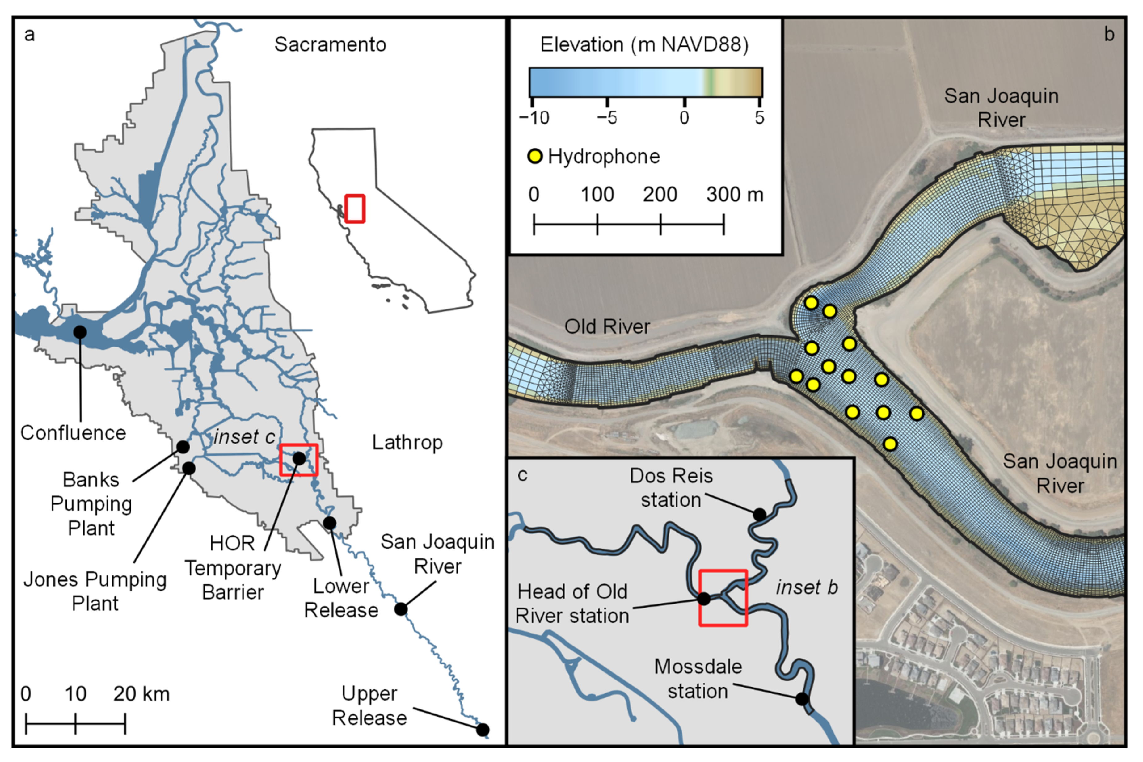
The Sacramento-San Joaquin Delta (Delta) (Figure 1) is a migration corridor and rearing habitat for juvenile Chinook salmon (Oncorhynchus tshawytscha) that emigrate from Central Valley rivers to the Pacific Ocean. Chinook salmon abundance in the Delta is a small fraction of historical abundance which once supported a large salmon fishery [1]. Chinook salmon abundance has decreased largely due to anthropogenic factors including decreased river flow during emigration [2], fragmentation and loss of habitat due to dam construction [1], entrainment in water diversion facilities [3], predation by non-native species [4], limited food supply and exposure to contaminants [3]. Within the Central Valley multiple races of Chinook salmon historically thrived. Today, winter-run Chinook are federally listed as an endangered species and spring-run Chinook are listed as threatened. Central Valley fall-run Chinook salmon are listed as a “species of concern” by NOAA Fisheries, leading to intensive efforts to quantify and understand Chinook salmon survival through the Delta [5]. Route-specific survival studies have concluded that survival through the San Joaquin River is considerably lower than other large river systems on the west coast of North America [5]. In addition, the potential migratory pathways of Chinook from the San Joaquin River through the Delta also differ in estimated survival rates [5]. However, the environmental conditions influencing emigrating smolt swimming behavior and the effect of this behavior on route selection are not well understood.
Acoustic telemetry data are useful in understanding pathways of emigrating Chinook salmon through the Delta and studies have shown that mortality varies with migration route [6,7]. Acoustic telemetry has also shown that fish are not homogeneously distributed in channels and therefore the proportion of fish entering a specific channel at a divergent junction (diffluence) can be different from the proportion of flow entering that channel [8]. This difference indicates the importance of swimming. However, unless collected concurrently with highly detailed hydrodynamic data, the contribution of fish swimming velocity to velocity over ground and consequently route selection is unclear. Furthermore, telemetry data is only diagnostic and cannot be directly used to evaluate engineering projects aimed at improving Chinook salmon survival. In contrast, a behavioral particle-tracking model (PTM) can predict route selection for proposed management alternatives that have no historical precedent.
Our study site at the junction of the San Joaquin River and Old River (Figure 1) is of great interest both because the Old River route has a high risk of Chinook salmon entrainment in water diversion facilities [5] and because of high predator density [9]. While routing into Old River increases the entrainment risk, routing down the San Joaquin River is associated with high predation losses, and includes a reach with the highest predation risk in the South Delta observed during a single wet year study [10]. The dominant predator of Chinook salmon smolts in this region is striped bass (Morone saxatilis) [11] and other known predators include largemouth bass and catfishes [12]. Overall, Central Valley Chinook salmon emigration survival can vary strongly interannually with river flow with lowest survival during dry years [7,11]. In the highly managed San Francisco Estuary, management alternatives contemplated to aid survival of emigrating Central Valley Chinook salmon include timing and location of hatchery fish release, outflow (reservoir release) management, water diversion limitations, fish salvage facility operation, use of physical and non-physical barriers, channel modifications, predator removal and other actions. Given the range of management options, a reliable tool is needed to estimate the effectiveness of actions in improving outmigration survival.
As a component of a tool to estimate survival associated with management actions, a behavioral PTM that specifies varying swimming velocities of particles through time can estimate emigrating juvenile Chinook route selection for both historical conditions and proposed alternatives. In our analysis, swimming velocities estimated from acoustic telemetry data and three-dimensional hydrodynamic model results were used to infer swimming behavior of Chinook salmon. This study shares aspects of other swimming behavior analyses, such as the use of a hydrodynamic model in swimming speed estimates [13] and route selection studies, including the assumption of surface orientation [14] but we combined more aspects of observed behavior in our behavioral PTM than these previous studies. The most complex behavior formulation was a combination of surface orientation (maintaining a vertical position near the surface), constant rheotaxis and time-varying swimming. Probability density functions (PDFs) associated with a correlated random walk (CRW) formulation [15] were found to fit the distribution of estimated time-varying swimming velocities well. The behavioral PTM incorporating these behaviors with parameters consistent with telemetry data was then applied to estimate probabilistic route selection for each observed fish. The results from these models are useful to managers interested in understanding and managing routing of migrating salmon through complex estuarine ecosystems.
2. Materials and Methods
2.1. Site Description
The Sacramento-San Joaquin Delta (Delta) extends from where the confluence of the Sacramento River and the San Joaquin River meet Suisun Bay to the City of Sacramento on the Sacramento River and several kilometers south of Lathrop on the San Joaquin River (Figure 1). The study site is at the junction of the San Joaquin River and the head of Old River (HOR) located at the southern landward extreme of the Delta (Figure 1). In this tidally influenced freshwater region of the Delta, reversing tidal flows are muted during high flow periods. The climate is Mediterranean with the majority of rainfall occurring from November through April with large year-to-year variability in timing, magnitude and duration of precipitation. Flows are largely regulated by reservoirs in the San Joaquin Valley watershed. During typical flow conditions, most water entering Old River from the San Joaquin River is removed at major diversions—the C.W. Bill Jones Pumping Plant of the Central Valley Project (CVP), operated by the U.S. Bureau of Reclamation, and the Harvey O. Banks Pumping Plant of the State Water Project (SWP), operated by the California Department of Water Resources. Correspondingly, fish routing through Old River are at high risk of entrainment at the water export facilities, or predation near the facilities. A portion of the surviving smolts which arrive at the facilities are salvaged and trucked to the western boundary of the Delta where they are released back into the Estuary [2]. Except in years in which high flow prevents installation, a temporary rock barrier has been installed at the head of Old River during the spring period of emigrating Chinook salmon in order to reduce the passage of salmonids into Old River. In 2018 the structure was only partially installed, extending from the southern shoreline into but not across the channel (Figure 1).
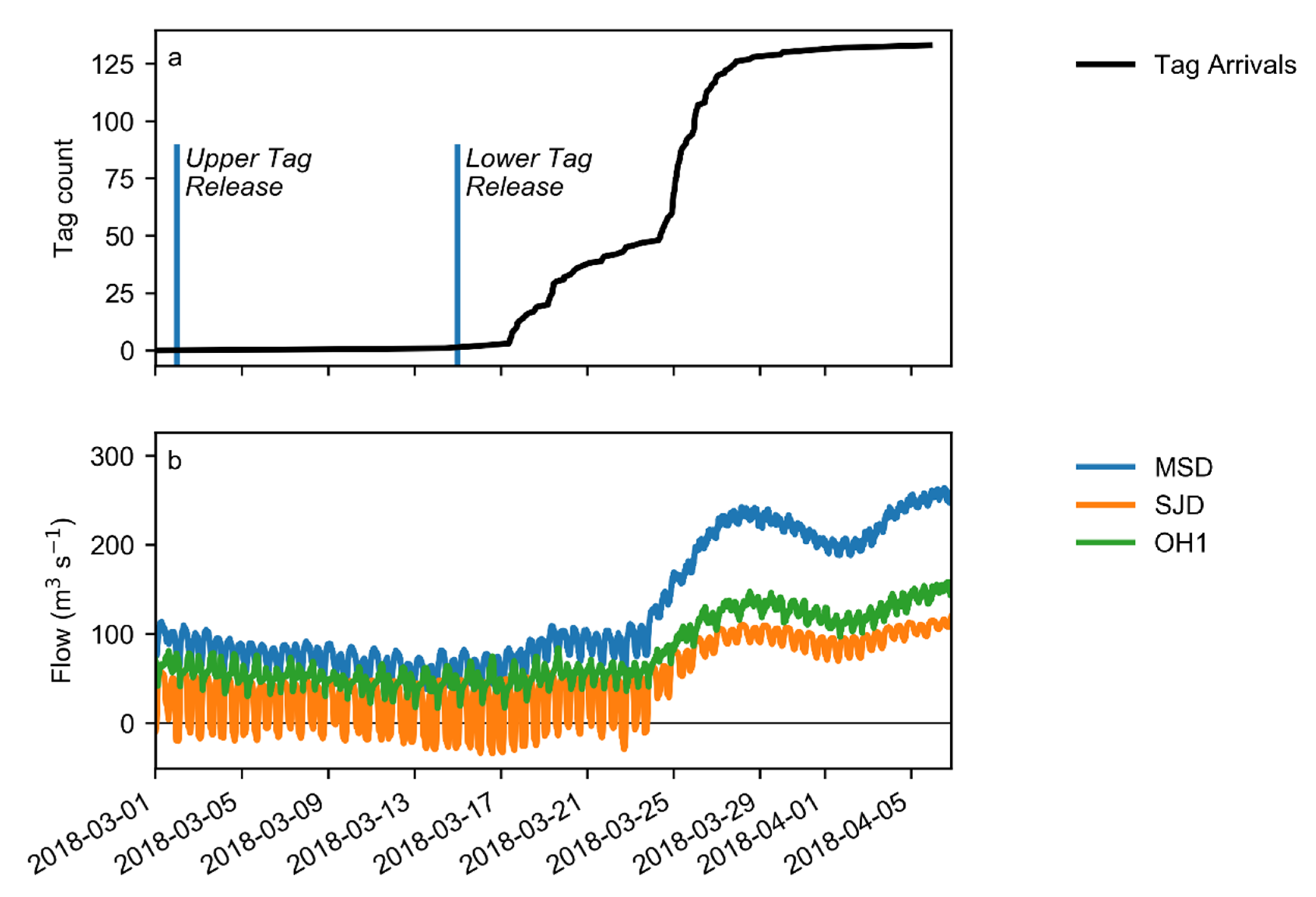
The study period was March–April 2018, timed to capture the emigration of Chinook smolts. River discharge, reported at Mossdale upstream of the junction and Dos Reis and Head of Old River downstream of the junction, was significant and variable during the study period (Figure 2). During the study period, a tidal signal was clear at all stations, though the flow direction reversed only at Dos Reis, and only during the lower flow period before 24 March.
2.2. Fish Release and Acoustic Telemetry
A total of 650 acoustically tagged, hatchery-reared smolts were released from two sites upstream of the study site: an upstream release site, 60 river km above the study site and a downstream release site, 14 river km above the study site (Figure 1). While fish from the upstream release traversed more of the historical migratory route down the San Joaquin River, in-river predation losses can be substantial in the reach from the release to the study site. The survival was 47% for a similar reach in 2009 [2] leading to the addition of the lower release site in order to ensure that sufficient numbers reached the study site. Releases occurred in March 2018, timed to coincide with the historical emigration season for sub-yearling, spring-run juveniles [1]. The upper release of 325 smolts occurred on 2 March 2018, and the lower release of 325 individuals occurred on 15 March 2018 (Figure 2). Data from acoustic receivers between the release sites allowed us to time the lower release to coincide with individuals arriving from the upper release.
Salmon smolts used in this study originated from the experimental population of spring-run Chinook reared at the California Department of Fish and Wildlife (CDFW) Salmon Conservation and Research Facility (SCARF), located at the base of Friant Dam, near Fresno, CA, USA. The water source for SCARF is the San Joaquin River resulting in a water chemistry and temperature similar to habitats where natural spawning and rearing could occur. Smolts were reared at SCARF until fish reached sizes sufficient to maintain a tag burden of ≤5% of total body weight, a minimum of 4.2 g for the 0.216 g Juvenile Salmon Acoustic Tracking System (JSATS) acoustic transmitter (model SS400, ATS Issanti, MN, USA). Smolt lengths and weights were measured at the time of acoustic tagging. Smolt length ranged from 71–86 mm fork length, with an average of 76.6 mm. Acoustic tagging of the smolts was performed by intraperitoneal implantation where a 2–3 mm incision was made 0.5–1 mm off the ventral midline, anterior to the pelvic girdle. After each tag was inserted, the incision was closed with a surgeon’s knot. Prior to the procedure fish were anesthetized with a bufferedsolution of tricaine methanesulfonate. Transport tanks were monitored for oxygen and temperature during the transport process. Temperature acclimation at the release site prior to release followed a protocol of adjusting by 2 °C per hour until the transport tank temperature equaled in-river temperatures. Additional details on methods of surgery and handling are described in [16].
A 416 kHz multi-dimensional positioning system by Teknologics, LLC, composed of an array of 13 hydrophones nominally spaced 70 m apart, was used to record pings from the tags. Horizontal tag positions were estimated using the YAPS software [17] at a 5-s interval. Additional information on the tagging and acoustic telemetry data for this study is available in [18].
2.3. Hydrodynamic Model
A high-resolution three-dimensional SUNTANS [19] hydrodynamic model was developed for the study site [18]. Typical lateral grid spacing of the unstructured grid in the region where telemetry data were available was 2–3 m, with somewhat larger edge lengths farther from the study area. The vertical dimension was discretized with 50 z-layers and a spacing of 0.27 m. The hydrodynamic model was calibrated against velocity transect data collected by an acoustic doppler current profiler (ADCP) at nine cross-sections in the study area. Additional information on model development and calibration is provided in [18]. In this study, the model domain was extended (Figure 1) from the domain in [18] in order to ensure that predicted route selection is not influenced by model extent.
2.4. Swimming Behavior Analysis
Tags included in the swimming behavior analysis had at least 10 detections with at least one detection below the junction. Tags that were detected in the array for more than 60 min or exhibiting average swim speeds > 0.5 m s−1 were assumed to be predators and discarded [18]. Detections more than 25 m upstream of the start of the array were discarded. Detections below the junction were used only in determining route selection and were not used for swim velocity estimates (due to poor hydrodynamic calibration below the junction).
For each of the 96 tags that fit these criteria, a swimming velocity was calculated for each pair of successive relocations from the telemetry data. For each pair of relocations, the hydrodynamic model-predicted velocity was averaged over the top 2 m of the water column at the midpoint location and time between relocations, and subtracted from the velocity over ground estimated from telemetry to get the swimming velocity,
where is the (horizontal) velocity over ground, is the hydrodynamic velocity, defined previously and is the swimming (behavior) velocity. Using this approach, and only considering relocations located upstream (landward) of the diffluence (junction with diverging flow in the downstream direction), a set of swimming velocities were estimated in [18].
We analyzed this set of horizontal swimming velocities to determine swimming parameters to use in a Chinook salmon smolt behavioral PTM. The swimming behavior approach was a combination of surface orientation, constant rheotaxis for each tagged smolt and a CRW which includes time-varying swimming speed and heading. The horizontal portion of this formulation was
where is the velocity associated with rheotaxis, with positive rheotaxis indicating upstream swimming, and is associated with the CRW. We assumed that rheotaxis speed was constant in time for each individual but the velocity associated with the CRW varied at each time step of the simulation. The streamwise hydrodynamic velocity direction is
where and are the unit vector components. Since, for a given hydrodynamic velocity, the direction of rheotaxis is known, Equation (2) can be rewritten
where is the strength of rheotaxis, is a swimming speed associated with the CRW, and is the unit vector describing the heading of swimming associated with the CRW.
The parameters of a CRW [15] were estimated from sequential changes in swimming velocity at each time step. The CRW was parameterized by a Weibull distribution for swimming speeds and a wrapped Cauchy distribution for turn angles. In order to estimate the parameters of these distributions, the swimming velocities were converted to a set of swimming speeds (i.e., the magnitude of ) and turn angles estimated as the difference in direction associated with the difference in velocity between two successive swimming velocity estimates.
where is the turn angle and is an arctangent function.
The pulse rate interval of the tags was 5 s and turn angles were estimated for that time interval. Swimming velocities were only estimated when valid relocations were available at this interval, not over longer intervals associated with missing relocations. A total of 3871 calculated turn angles were used in the analysis.
2.5. Analysis of the Effect of Position Error
Position error in the acoustic telemetry data can influence estimated swimming speeds and turn angles. Similarly, inaccuracies in the hydrodynamic model can influence the estimated swimming velocities. A median position uncertainty of 1.4 m was associated with the analysis of telemetry data [18]. However, because successive position errors were highly autocorrelated, and hydrodynamic model errors are also expected to be autocorrelated, the effect of position error on estimated speeds and turn angles may be small as only the uncorrelated position errors affect speed and turn angle calculations. In order to explore the effect of uncorrelated position error on the parameters of the behavior formulation, we generated synthetic position data with Gaussian position errors
where and are the synthetic cooordinates at time , is a Weibull random variable with shape parameter and scale parameter , and is a normal random variable with mean of zero and standard deviation . First synthetic tracks were determined assuming a constant heading () of zero and Weibull distribution parameters estimated from the telemetry data. Turn angle and speed distribution parameters were estimated for synthetic datasets with ranging from zero to 50 cm, following the same methods as for the telemetry data. Because the heading associated with behavior () was zero, any change in heading in the synthetic data results from position error.
After a bound of position error was estimated from that approach, Equation (7) was applied to generate synthetic positions from the combination of position error and a full CRW. We then fit a revised shape parameter , scale parameter , and turn angle parameter , associated with the combination of swimming behavior and position error. In contrast to estimates of these parameters directly from the telemetry data, this approach provides an estimate of actual swimming accounting roughly for the effect of position error.
2.6. Behavior Formulation
A set of proposed behavior formulations combining the aspects of behavior observed in the telemetry data and assumed vertical distribution were implemented and the route selection resulting from each were evaluated. The components of behavior representations were surface orientation, rheotaxis and a continuous random walk. Each behavior formulation was a combination of these individual components.
The velocity of each particle, representative of an individual fish, at each time step in the model was the sum of the hydrodynamic velocity and the swimming velocity:
where is the two-dimensional vector of predicted horizontal fish velocity over ground, is the predicted hydrodynamic velocity and is the predicted swimming (behavior) velocity, all at time step in the behavioral PTM. The swimming velocity and other properties associated with each particle were updated at a 5 s interval.
The predicted swimming velocities in Equation (8) at time step were specified according to the statistical distributions fit in the telemetry data analysis, resulting in the equation
where is a normally distributed variable with mean , standard deviation , and is a Weibull random variable with shape parameter , and scale parameter . In the behavioral PTM simulations the rheotactic speed at any point in time and space was limited to 50% of the downstream hydrodynamic velocity and the speed applied in the CRW was capped at 0.5 m s−1 to only allow physiologically realistic swimming speeds, consistent with estimates of swimming speeds [18]. The unit vector was updated at each time step based on the heading
where is a wrapped Cauchy-distributed variable with scale parameter and an implied peak position of zero. Upon encountering the shoreline, any component of the heading onto land was reset so that the swimming is along shore. Note that the correlated aspect of the CRW was the heading which was perturbed by the wrapped Cauchy distributed variable. In contrast the swimming speed component of the CRW was independent between time steps. The rheotaxis remained constant for each particle during the simulation, according to the normal random number drawn for that particle.
The vertical position of passive particles varied due to vertical advection and diffusion. The vertical aspect of the behaviors implemented was surface orientation in which a vertical position was specified which corresponds to vertical distance from the water surface to a particle. Each particle was assigned a unique vertical position drawn from a uniform random distribution in the range of 0.25 to 2 m, consistent with a depth range over which predicted hydrodynamic velocity was averaged in the analysis of swimming velocity [18]. In shallow water, the depth from the surface was not allowed to be in the lowest 25% of the water column. Therefore, for example, in a 1 m deep water column, a particle with a target depth of 1.2 m below the water surface would be reassigned a depth of 0.75 m below the water surface (0.25 m above the bed).
2.7. Behavioral Particle-Tracking Model Simulations
Modeling scenarios were performed for a set of hypothesized behaviors. The three behavior components are surface orientation, rheotaxis and a correlated random walk (CRW) described previously. Combinations of these three components are explored (see Table 1). The combinations of behavior components are formed by linear superposition of individual components. For example, the combined effect of rheotaxis and a CRW results from addition of the swimming velocity associated with rheotaxis to the velocity associated with the CRW. The base behavior was passive particles and the most complex behavior included surface orientation, rheotaxis and CRW. The remaining six behaviors included a subset of the behavior components. For each tag and each behavior, 1000 particles were released at the location and time of the first detection of the tag in the array.
For each behavior scenario and each tag, 1000 particles were released at the location of the first detection of each tag. Each particle was tracked for 12 h though most particles transit the acoustic array in approximately 10 min.
The particle-tracking model (PTM) component of the behavioral PTM calculates three-dimensional particle trajectories using hydrodynamic velocity and eddy diffusivity predicted from the three-dimensional hydrodynamic simulation [20] and the swimming velocity according to the formulation described previously. Vertical diffusion was represented by the Milstein scheme [21] as recommended in [22], and the time step for diffusion was specified following [23]. Note that the vertical diffusion did not influence the vertical position of particles for the surface-oriented behavior. A constant horizontal diffusion of 0.01 m2 s−1 was applied, consistent with turbulent diffusivity estimated from scaling relationships [24]. The hydrodynamic velocity field was output from the hydrodynamic model at a 15 min interval and swim velocities and particle positions were estimated at a 5 s interval, corresponding to the 5 s pulse interval for the tags.
2.8. Swimming Behavior Evaluation
The behavioral PTM calculated route selection of each particle that transited past the diffluence based on the initial transit, consistent with the determination of observed route selection from telemetry data. Only tags that were detected at the diffluence were included in this analysis. The fraction of particles consistent with the route selection of the tag was tabulated for each behavior. Only particles that transit the diffluence were counted.
The probability of the observed route selection given the particle tracking results for each behavior was evaluated with a likelihood metric corresponding to a binomial distribution. For example, for a single observed tag, if 600 of the associated particles took the Old River route and 400 took the San Joaquin River route at the diffluence, the probability associated with an observed route selection of Old River would be 0.6. This is multiplied for each tag to form an overall likelihood quantifying the consistency of the behavioral PTM results with acoustic telemetry data,
where is the likelihood of behavior , is the probability of the observed route occurring based on the predicted routes for behavior , and ntags is the number of tagged salmon smolts in the dataset. A lower bound on the probability of 0.001, the reciprocal of the number of particles released per tag, was included to ensure that the likelihood did not become zero in the (rare) case in which none of the particles for a behavior had the same route selection as the observed route for a given tag.
In addition to this likelihood metric, we report the predicted fraction of particles taking the HOR route, the bias towards the HOR route relative to the observations, and the fraction of predicted routes consistent with corresponding observed routes. The bias is calculated as the fraction of false positive predictions of the HOR route (particles predicted to take the HOR route for tags observed taking the SJ route) minus the false positive predictions of the SJ route.
3. Results
3.1. Swimming Behavior Parameters
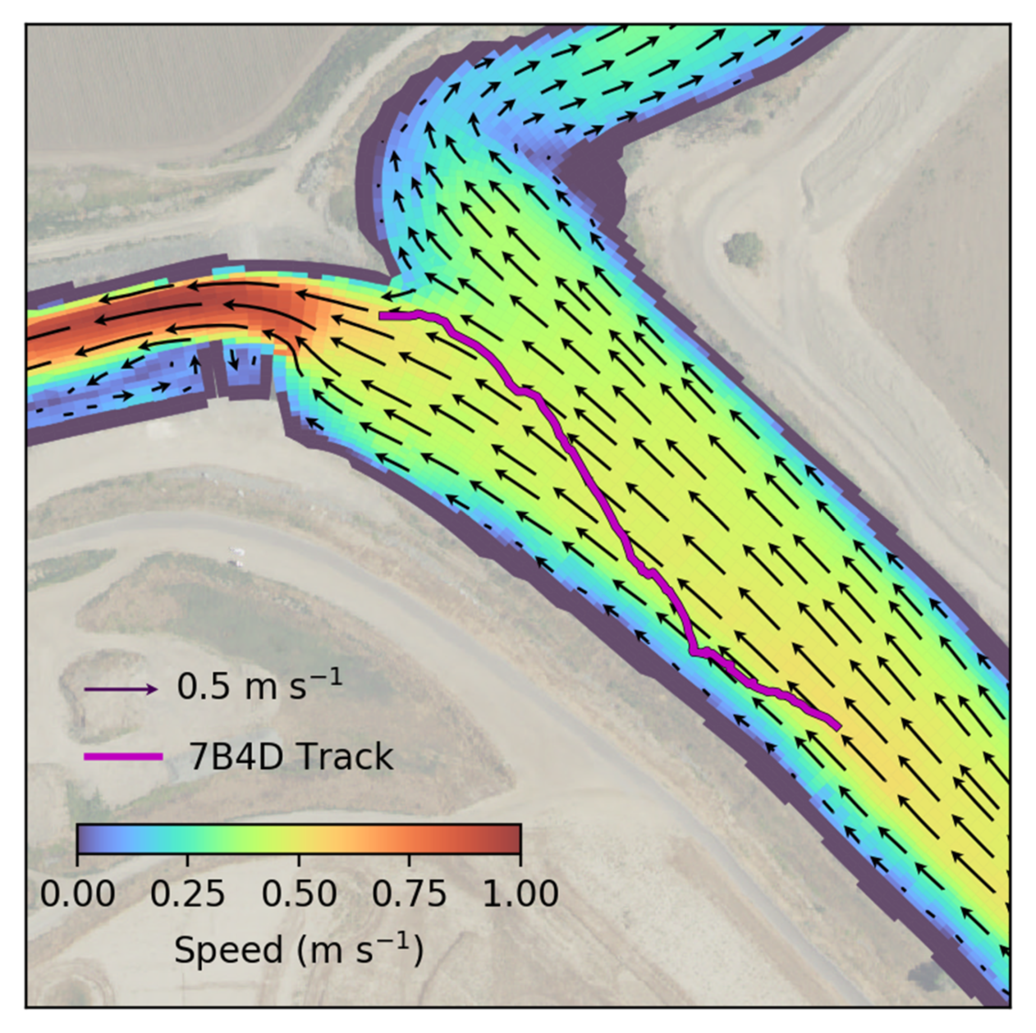
Equation (1) was applied to estimate swimming speed for each pair of relocations at a 5-s interval. As an example of the hydrodynamic information used in this approach, the near-surface hydrodynamic velocities predicted on 19 March 2018 at 4:26 a.m., at the time of transit of tag 7B4D, is shown in Figure 3.
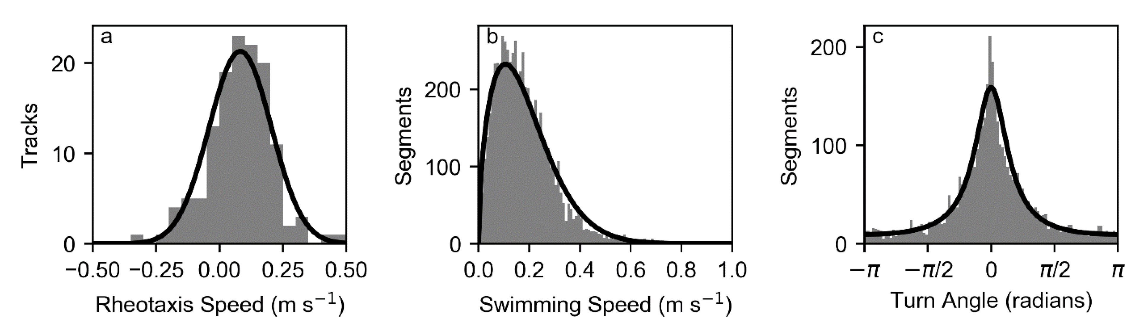
An average rheotactic velocity was calculated for each individual tag. These were combined to form a histogram which was fit with a normal distribution having mean of 0.0819 m s−1 and standard deviation of 0.123 m s−1. Positive rheotaxis was more common than negative rheotaxis (Figure 4a).
The distribution of swimming speed for each pair of consecutive relocations at a 5 s interval was fit with a Weibull distribution (Figure 4b) resulting in a of 1.56 and of 0.205 m s−1. The turn angle was estimated for each consecutive pair of heading estimates at a 5 s interval and the distribution was fit with a wrapped Cauchy distribution (Figure 4c) resulting in an estimated of 0.608.
3.2. Analysis of the Effect of Position Error
Equation (7) was used to quantify the effect of position error on estimated turn angles. In preliminary exploration, the wrapped Cauchy turn angle parameter was the parameter most sensitive to position error. Therefore, we generated synthetic data with no change in heading in the CRW formulation (turn angle of zero) so that estimated turn angles in analysis of the synthetic positions resulted solely from position error. The best fit CRW determined for each value of position error and the parameter which varied most strongly with assumed position error was , which increased roughly linearly with position error. At an assumed standard deviation of position error () of 18 cm, the estimated Cauchy from fitting the distribution of synthetically-generated turn angles associated with Equation (7) was smaller than what was estimated from the observed position estimates. This indicated larger turns from position error of 18 cm than the turns based on the telemetry data-based swimming speed analysis. Conditional primarily upon the assumption of normally distributed position error, this analysis suggests that the actual uncorrelated position error was smaller than 18 cm. The distributions of swimming speed and turn angle from the synthetic data including position error were well described by Weibull and wrapped Cauchy distributions, respectively. For that reason, fitting a position error parameter and behavior parameters simultaneously based on the telemetry data would lead to confounding of parameters in our specific behavior formulation.
Given the estimated upper bound on uncorrelated position error of 18 cm, a position error of 10 cm was assumed and revised CRW parameters were fit, resulting in of 0.774, of 1.47, and of 0.198. The revised parameters are associated with lower swimming speed and smaller turns than the estimates of parameters which did not account for the effect of position error.
3.3. Behavioral Particle-Tracking Model Results
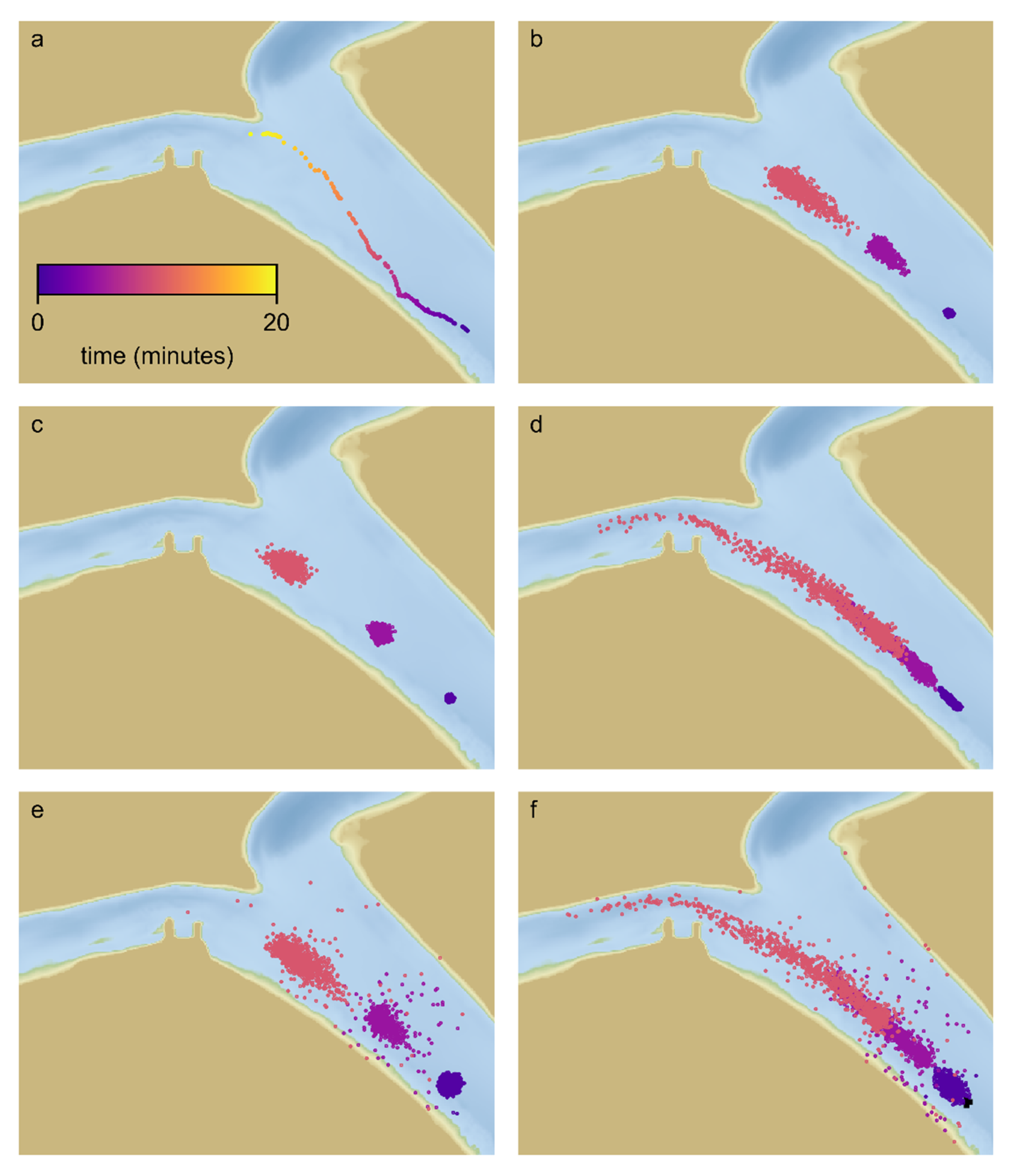
The behavioral PTM predicted position at a 5 s interval for each of 1000 particles for eight different behavior formulations for each of 96 tags. As an example, position estimates for tag 7B4D are shown in Figure 5. This tag enters the acoustic array towards river left (Figure 5a) on 19 March 2018 at 4:17 p.m., transits the array in 21 min, and exits into Old River.
For each behavior formulation, 1000 particles were introduced at the time and location of the entry of each tag to the acoustic array (specifically the first detection not more than 25 m upstream of the receivers). Passive particles for the example tag 7B4D were transported downstream and started arriving at the confluence in roughly 10 min (Figure 5b). The horizontal spreading of the particles was due to horizontal turbulent diffusion and vertical shear dispersion associated with vertical variability in velocity, which caused particles near the bed to be advected more slowly than particles at the surface. Shear dispersion can also act laterally when lateral velocities, such as secondary circulation velocities, are present.
The surface-oriented behavior particles were distributed from 0.25 m to 2 m below the water surface. This surface orientation resulted in less shear dispersion and faster downstream advection of most particles (Figure 5c). In cases where secondary circulation is present, surface-orientation can be expected to result in accumulation of particles at the outside of bends. Given that minimal secondary circulation was observed in the ADCP observations or the hydrodynamic model [18] in this region, the behavioral PTM predictions did not show strong accumulation at the outside of bends or other specific lateral position. However, it should be noted that the hydrodynamic model estimated substantial secondary circulation in bends of the San Joaquin River upstream of the junction.
In the rheotaxis behavior formulation, each particle was assigned a static rheotaxis speed for the duration of the simulation. Because the speed drawn varies among particles, this behavior resulted in a larger longitudinal spread in particles (Figure 5d) but no increase in lateral spreading relative to passive particles (Figure 5a). Since the mean of the rheotaxis speed distribution (Figure 4) was positive (upstream swimming), rheotaxis generally results in slower mean downstream transport relative to passive particles.
In the CRW behavior, each particle updated its swimming speed and direction at a 5-s time interval. This resulted in a more dispersed particle distribution (Figure 5e) relative to passive particles (Figure 5b), particularly in the lateral direction.
The combined behavior included surface orientation, rheotaxis and a CRW. It resulted in the most dispersed distribution by combining the strong longitudinal spreading associated with variable rheotaxis and horizontal spreading associated with the CRW (Figure 5f).
3.4. Swimming Behavior Evaluation
The route selection of the tagged salmon smolts was strongly dependent on entry location (Figure 6a). However, for a given entry position, either route is possible. For example, tags which enter river right (the right side of the river for an observer looking downstream) sometimes have Old River route selection, which could be expected during periods of flow reversal on the San Joaquin River (Figure 2). The route selection of individuals (particles) with active behavior (Figure 6b) was less uniform than passive particle route selection for a given entry location. Given that 1000 particles were introduced at each entry location, the tagged fish route selection can be viewed as an individual realization of route selection for a given entry location. The route selection of each particle involves a degree of stochasticity due to random components of swimming including the speeds and directions selected in a CRW formulation, the rheotaxis speed selected and the distance to the surface. Stochasticity in route selection is also contributed by the diffusion term of the particle-tracking model representing the effect of turbulent motions.
The route selection for each particle was determined by the first transit past the diffluence into Old River or the San Joaquin River. Table 1 presents several metrics of particle route selection and comparisons between particle and tag route selection. “HOR Fraction” is the fraction of particles (averaged over all particle entry points) taking the HOR route, and the similarity across behaviors indicates that average route selection was similar for all behaviors. The behavior in which most particles selected the same route as the tagged smolts they represent (summarized in the Fraction Consistent column) was surface orientation. However, all behaviors produced similar values of this metric. The values of the likelihood metric spanned from ~10−79 for the rheotaxis behavior, with a similar value for passive particles, to ~10−40 for the most complex behavior, which included surface orientation, rheotaxis and a CRW. CRW has the largest likelihood metric for a single behavior component. This primarily suggests that more complex behaviors were less likely to produce route selection estimates strongly inconsistent with the observed route selection of a tag. This is expected for the behavior formulations including the CRW component which is likely to disperse particles and avoid cases in which no particles follow a route consistent with the associated tag. Greater likelihood metrics were also associated with surface orientation and rheotaxis indicating some support for those behaviors. A notable trend of the particle-tracking results is to overestimate head of Old River route selection (Table 1). This may be due to imprecise predictions of flow into each junction, which is strongly controlled by boundary conditions using measured flow observations which themselves may be imprecise. The bias in estimated route selection may also be influenced by lower detection efficiency of the acoustic array in Old River downstream of the diffluence. Lack of detection downstream of the diffluence resulted in exclusion from the dataset used in this analysis, leading to under-representation of tags with Old River route in the dataset. The lowest estimated HOR Bias metric is for the surface orientation and rheotaxis behavior.
4. Discussion
Behavioral PTM models and individual-based models can represent fish movement by a wide range of approaches [25]. One approach is to specify instantaneous swimming velocity through time which can vary in response to hydrodynamic or other environmental conditions [13,26]. In some cases, the only data available indicating the distribution of fish through time is trawl data collected at monthly or other coarse time intervals. In that case, hypothesized behavior formulations can be evaluated based on the consistency of predicted distribution with catch data from trawls [27]. In contrast, acoustic telemetry data collected at a time interval of several seconds, combined with hydrodynamic modeling, allows estimation of instantaneous swimming behavior of salmon at small spatial scales [13]. The swimming speed can be further analyzed to provide swimming behavior formulations with instantaneous swimming velocities. This provides a swimming behavior formulation with instantaneous velocities directly supported by observations. Here we used the telemetry data both to inform the representation of instantaneous swimming and also to evaluate the ability of each behavior formulation to reproduce observed route selection.
The statistical distribution of estimated swimming speeds from the combined use of acoustic telemetry data and three-dimensional hydrodynamic modeling was well-represented by a Weibull distribution, and turn angles were well-represented by a wrapped Cauchy distribution, as used in other animal movement representations [15]. There was evidence that the swimming speed at subsequent 5 s intervals was autocorrelated, but this autocorrelation was not strong. The proposed behavior formulations could be extended in future work to account for autocorrelation in speed, particularly given a larger acoustic telemetry dataset. Data could also be analyzed to identify multiple behavioral states [28] allowing state switches over time. However, due to the limited quantity of telemetry data, particularly because a typical duration between first detection and exit from the array is 15 min, it would be challenging to identify changes in behavioral state from the present data.
On average, the route selection of the particles was fairly consistent with observed route selection for all behavior formulations. However, the likelihood metric estimated for each behavior formulation (Table 1) indicates that passive behavior is the least likely behavior formulation. We conclude that, although the route selection of passive particles often matches the observed route, the observed route selection of some individual tags was unlikely to result from passive behavior, and that active behavior influences route selection. This is consistent with findings of [14] which indicated that surface orientation would influence route selection at a channel junction along a bend. Our study area is one that would not be expected to have as large an influence of surface orientation on route selection because the channel leading up to the diffluence is relatively straight so surface-oriented particles may be expected to be fairly uniformly distributed laterally.
Due to the small spatial extent of our study, we caution against generalization of the route selection results. Additional particle-tracking and behavioral PTM modeling with particle releases further upstream (not reported here) showed strong differences in route selection between the surface-orientation behavior and passive particles. The observed vertical positions of Chinook salmon smolts could not be reliably calculated in this study but vertical position observations would be a useful addition to future studies. In addition, extending the study to resolve lateral distribution of tags upstream of the first bend upstream of the diffluence may lead to strongly different conclusions about the importance of behaviors on route selection.
These results inform understanding of swimming behavior and potential management of juvenile Chinook salmon. For example, the conclusion that smolts were not behaving as passive particles, consistent with previous work [13], is important for managers because it suggests that actions such as non-physical barriers that influence salmon smolt behavior may increase survival by influencing route selection. We did not investigate the drivers of smolt behavior in this paper, however we do suggest that multi-dimensional tracking systems such as that used in this study could be leveraged to disentangle these dynamics. Future work will be critical in understanding the drivers of juvenile salmon behavior and the extent to which managers can affect behavior and routing. Such results would certainly be valuable in California but could also hold value across the Pacific and Atlantic Coasts where juvenile salmon migrations and management are similarly affected by human activity.
Author Contributions
Conceptualization, E.S.G., R.C.H. and M.J.T.; Methodology, E.S.G., R.C.H. and M.J.T.; Software, E.S.G. and R.C.H.; Validation, E.S.G.; Investigation, E.S.G., R.C.H. and M.J.T.; Resources, M.J.T., N.A.F. and A.L.R.; Data Curation, R.C.H. and M.J.T.; Writing—original draft preparation, E.S.G.; Writing—Review and editing, E.S.G., R.C.H., M.J.T., N.A.F. and A.L.R.; Visualization, E.S.G. and R.C.H.; Supervision, N.A.F.; Project administration, N.A.F.; Funding acquisition, N.A.F. and E.S.G. All authors have read and agreed to the published version of the manuscript.
Funding
This research was funded by California Department of Fish and Wildlife under Proposition 1—Delta Water Quality and Ecosystem Restoration Grant Program, Agreement P1796017-00. NAF and ALR were supported by the Agricultural Experiment Station of the University of California, Project CA-D-WFB-2098-H and CA-D-WFB-2467-H, respectively. ALR is also supported by the California Trout and Peter B. Moyle Endowment for Coldwater Fish Conservation.
Institutional Review Board Statement
Fish tagging was performed under ESA Section 10(a)(1)(A) permit #20571, and adhered to the policies of University IACUC #21614.
Informed Consent Statement
Not applicable.
Data Availability Statement
Telemetry and ADCP data are available at Holleman Rusty, Gross Edward, Thomas Michael, Rypel Andrew, Fangue Nann (2021). Hydrodynamic and salmon smolt telemetry at the Head of Old River, California. SEANOE. https://doi.org/10.17882/80285.
Acknowledgments
The authors thank Pete Klimley for contributions to the original study objectives and design. Scott Burdick created GIS images used in figures.
Conflicts of Interest
The authors declare no conflict of interest.
References
- Yoshiyama, R.M.; Fisher, F.W.; Moyle, P.B. Historical Abundance and Decline of Chinook Salmon in the Central Valley Region of California. N. Am. J. Fish. Manag. 1998, 18, 487–521. [Google Scholar] [CrossRef]
- Buchanan, R.A.; Skalski, J.R.; Brandes, P.L.; Fuller, A. Route Use and Survival of Juvenile Chinook Salmon through the San Joaquin River Delta. N. Am. J. Fish. Manag. 2013, 33, 216–229. [Google Scholar] [CrossRef]
- Jahn, A.; Kier, W. Reconsidering the Estimation of Salmon Mortality Caused by the State and Federal Water Export Facilities in the Sacramento–San Joaquin Delta, San Francisco Estuary. SFEWS 2020, 18. [Google Scholar] [CrossRef]
- Stompe, D.; Roberts, J.; Estrada, C.; Keller, D.; Balfour, N.; Banet, A. Sacramento River Predator Diet Analysis: A Comparative Study. SFEWS 2020, 18. [Google Scholar] [CrossRef] [Green Version]
- Buchanan, R.A.; Brandes, P.L.; Skalski, J.R. Survival of Juvenile Fall-Run Chinook Salmon through the San Joaquin River Delta, California, 2010–2015. N. Am. J. Fish. Manag. 2018, 38, 663–679. [Google Scholar] [CrossRef]
- Perry, R.W.; Skalski, J.R.; Brandes, P.L.; Sandstrom, P.T.; Klimley, A.P.; Ammann, A.; MacFarlane, B. Estimating Survival and Migration Route Probabilities of Juvenile Chinook Salmon in the Sacramento–San Joaquin River Delta. N. Am. J. Fish. Manag. 2010, 30, 142–156. [Google Scholar] [CrossRef]
- Singer, G.P.; Chapman, E.D.; Ammann, A.J.; Klimley, A.P.; Rypel, A.L.; Fangue, N.A. Historic Drought Influences Outmigration Dynamics of Juvenile Fall and Spring-Run Chinook Salmon. Environ. Biol. Fish 2020, 103, 543–559. [Google Scholar] [CrossRef]
- Romine, J.; Perry, R.; Blake, A.; Burau, J. Effects of Tidally Varying River Flow on Entrainment of Juvenile Salmon into Sutter and Steamboat Sloughs. SFEWS 2020, 19. [Google Scholar] [CrossRef]
- Michel, C.J.; Smith, J.M.; Lehman, B.M.; Demetras, N.J.; Huff, D.D.; Brandes, P.L.; Israel, J.A.; Quinn, T.P.; Hayes, S.A. Limitations of Active Removal to Manage Predatory Fish Populations. N. Am. J. Fish. Manag. 2020, 40, 3–16. [Google Scholar] [CrossRef]
- Michel, C.J.; Henderson, M.J.; Loomis, C.M.; Smith, J.M.; Demetras, N.J.; Iglesias, I.S.; Lehman, B.M.; Huff, D.D. Fish Predation on a Landscape Scale. Ecosphere 2020, 11. [Google Scholar] [CrossRef]
- Michel, C.J. Decoupling Outmigration from Marine Survival Indicates Outsized Influence of Streamflow on Cohort Success for California’s Chinook Salmon Populations. Can. J. Fish. Aquat. Sci. 2019, 76, 1398–1410. [Google Scholar] [CrossRef]
- Lehman, B.; Huff, D.D.; Hayes, S.A.; Lindley, S.T. Relationships between Chinook Salmon Swimming Performance and Water Quality in the San Joaquin River, California. Trans. Am. Fish. Soc. 2017, 146, 349–358. [Google Scholar] [CrossRef] [Green Version]
- Olivetti, S.; Gil, M.A.; Sridharan, V.K.; Hein, A.M.; Shepard, E. Merging Computational Fluid Dynamics and Machine Learning to Reveal Animal Migration Strategies. Methods Ecol. Evol. 2021, 12, 1186–1200. [Google Scholar] [CrossRef]
- Ramón, C.L.; Acosta, M.; Rueda, F.J. Hydrodynamic Drivers of Juvenile-Salmon Out-Migration in the Sacramento River: Secondary Circulation. J. Hydraul. Eng. 2018, 144, 04018042. [Google Scholar] [CrossRef]
- Morales, J.M.; Haydon, D.T.; Frair, J.; Holsinger, K.E.; Fryxell, J.M. Extracting More Out of Relocation Data: Building: Building Movement Models as Mixtures of Random Walks. Ecology 2004, 85, 2436–2445. [Google Scholar] [CrossRef] [Green Version]
- Singer, G.P.; Hansen, M.J.; Ho, K.V.; Lee, K.W.; Cocherell, D.E.; Peter Klimley, A.; Rypel, A.L.; Fangue, N.A. Behavioral Response of Juvenile Chinook Salmon to Surgical Implantation of Micro-acoustic Transmitters. Trans. Am. Fish Soc. 2019, 148, 480–492. [Google Scholar] [CrossRef]
- Baktoft, H.; Gjelland, K.Ø.; Økland, F.; Thygesen, U.H. Positioning of Aquatic Animals Based on Time-of-Arrival and Random Walk Models Using YAPS (Yet Another Positioning Solver). Sci. Rep. 2017, 7, 14294. [Google Scholar] [CrossRef] [PubMed] [Green Version]
- Holleman, R.C.; Gross, E.S.; Thomas, M.J.; Rypel, A.L.; Fangue, N.A. Swimming Behavior of Emigrating Chinook Salmon Smolts. PLoS ONE 2021. submitted. [Google Scholar]
- Fringer, O.B.; Gross, E.S.; Meuleners, M.; Ivey, G.N. Coupled ROMS-SUNTANS Simulations of Highly Nonlinear Internal Gravity Waves on the Australian Northwest Shelf. In Proceedings of the 6th International Symposium on Stratified Flows, Perth, Australia, 11–14 December 2006; pp. 533–538. [Google Scholar]
- Ketefian, G.S.; Gross, E.S.; Stelling, G.S. Accurate and Consistent Particle Tracking on Unstructured Grids: Particle Tracking on Unstructured Grids. Int. J. Numer. Methods Fluids 2016, 80, 648–665. [Google Scholar] [CrossRef]
- Milstein, G.N. A Method of Second-Order Accuracy Integration of Stochastic Differential Equations. Theory Probab. Its Appl. 1979, 23, 396–401. [Google Scholar] [CrossRef]
- Gräwe, U.; Deleersnijder, E.; Heemink, A.W. Why the Euler Scheme in Particle Tracking Is Not Enough: The Shallow-Sea Pycnocline Test Case. Ocean Dyn. 2012, 62, 501–514. [Google Scholar] [CrossRef]
- Shah, S.H.A.M.; Heemink, A.W.; Gräwe, U.; Deleersnijder, E. Adaptive Time Stepping Algorithm for Lagrangian Transport Models: Theory and Idealised Test Cases. Ocean Model. 2013, 68, 9–21. [Google Scholar] [CrossRef]
- Fischer, H.B. (Ed.) Mixing in Inland and Coastal Waters; Academic Press: New York, NY, USA, 1979; ISBN 978-0-12-258150-2. [Google Scholar]
- Rose, K.A.; Allen, J.I.; Artioli, Y.; Barange, M.; Blackford, J.; Carlotti, F.; Cropp, R.; Daewel, U.; Edwards, K.; Flynn, K.; et al. End-To-End Models for the Analysis of Marine Ecosystems: Challenges, Issues, and Next Steps. Mar. Coast. Fish. 2010, 2, 115–130. [Google Scholar] [CrossRef] [Green Version]
- Goodwin, R.A.; Politano, M.; Garvin, J.W.; Nestler, J.M.; Hay, D.; Anderson, J.J.; Weber, L.J.; Dimperio, E.; Smith, D.L.; Timko, M. Fish Navigation of Large Dams Emerges from Their Modulation of Flow Field Experience. Proc. Natl. Acad. Sci. USA 2014, 111, 5277–5282. [Google Scholar] [CrossRef] [PubMed] [Green Version]
- Korman, J.; Gross, E.; Grimaldo, L. Statistical Evaluation of Behavior and Population Dynamics Models Predicting Movement and Proportional Entrainment Loss of Adult Delta Smelt in the Sacramento–San Joaquin River Delta. SFEWS 2021, 19. [Google Scholar] [CrossRef]
- Gurarie, E.; Fleming, C.H.; Fagan, W.F.; Laidre, K.L.; Hernández-Pliego, J.; Ovaskainen, O. Correlated Velocity Models as a Fundamental Unit of Animal Movement: Synthesis and Applications. Mov. Ecol. 2017, 5, 13. [Google Scholar] [CrossRef] [PubMed] [Green Version]
Figure 1.
(a) Locations of interest including smolt release locations, with the extent of the Sacramento-San Joaquin Delta in grey shading; (b) computational grid, bathymetry and hydrophone location near the junction of the San Joaquin River and Old River; (c) the extent of the hydrodynamic model domain in black outline and the locations of flow observation stations.

Figure 2.
Chronology of (a) tagged fish release and cumulative arrival in the study area, and (b) measured flow upstream of the diffluence at Mossdale (MSD), downstream of the diffluence on the San Joaquin River at Dos Reis (SJD) and downstream of the diffluence on Old River (OH1).
Figure 2.
Chronology of (a) tagged fish release and cumulative arrival in the study area, and (b) measured flow upstream of the diffluence at Mossdale (MSD), downstream of the diffluence on the San Joaquin River at Dos Reis (SJD) and downstream of the diffluence on Old River (OH1).

Figure 3.
Predicted hydrodynamic speed (colors) and velocity (arrows) fields averaged from the surface to 2 m below the surface on 19 March 2018 at 4:26 a.m., at the time of transit of tag 7B4D. The observed path of tag 7B4D in the acoustic array is shown by the magenta line.
Figure 3.
Predicted hydrodynamic speed (colors) and velocity (arrows) fields averaged from the surface to 2 m below the surface on 19 March 2018 at 4:26 a.m., at the time of transit of tag 7B4D. The observed path of tag 7B4D in the acoustic array is shown by the magenta line.

Figure 4.
Histograms and corresponding best fit statistical distributions of swimming behavior components fit to swimming speeds estimated from position dataset: (a) rheotaxis speed, with positive indicating upstream swimming; (b) swimming speed of CRW; (c) turn angle of CRW.
Figure 4.
Histograms and corresponding best fit statistical distributions of swimming behavior components fit to swimming speeds estimated from position dataset: (a) rheotaxis speed, with positive indicating upstream swimming; (b) swimming speed of CRW; (c) turn angle of CRW.

Figure 5.
Observed and predicted positions for tag 7B4D: (a) position estimates of tag 7B4D and time from entry to acoustic array; (b–f) distributions of particles at 1 min (blue), 5 min (magenta) and 10 min (salmon) for; (b) passive; (c) surface-oriented; (d) rheotaxis; (e) CRW; (f) combination of surface-oriented, rheotaxis and CRW.

Figure 6.
Entry points and associated route selection of salmon (marker shape) and particles (marker color) where yellow indicates roughly 50% Old River route selection for: (a) passive particles; (b) combined behavior of surface orientation, rheotaxis and CRW.
Figure 6.
Entry points and associated route selection of salmon (marker shape) and particles (marker color) where yellow indicates roughly 50% Old River route selection for: (a) passive particles; (b) combined behavior of surface orientation, rheotaxis and CRW.


Table 1.
Route selection and behavior evaluation metrics across all tags for each behavior formulation. HOR Fraction is the fraction of particles that have head of Old River route selection; Likelihood reports the metric described by Equation (11); Fraction Consistent reports the fraction of particles with route selection consistent with their associated tag; HOR Bias reports the difference between the fraction of particles with HOR route selection for tags with San Joaquin River route selection minus the fraction of particles with San Joaquin Route selection for tags with HOR route selection.
| Behavior | HOR Fraction | Likelihood | Fraction Consistent | HOR Bias |
|---|---|---|---|---|
| Passive | 0.438 | 2.17 × 10−79 | 0.698 | 0.125 |
| Surface Orientation (SO) | 0.430 | 1.42 × 10−76 | 0.710 | 0.117 |
| Rheotaxis (R) | 0.436 | 1.02 × 10−79 | 0.693 | 0.123 |
| Correlated Random Walk (CRW) | 0.443 | 1.13 × 10−43 | 0.691 | 0.130 |
| SO + R | 0.428 | 3.75 × 10−75 | 0.705 | 0.116 |
| SO + CRW | 0.444 | 1.98 × 10−41 | 0.700 | 0.132 |
| R + CRW | 0.448 | 1.16 × 10−44 | 0.683 | 0.135 |
| SO + R + CRW | 0.449 | 1.35 × 10−40 | 0.690 | 0.136 |
Publisher’s Note: MDPI stays neutral with regard to jurisdictional claims in published maps and institutional affiliations. |
© 2021 by the authors. Licensee MDPI, Basel, Switzerland. This article is an open access article distributed under the terms and conditions of the Creative Commons Attribution (CC BY) license (https://creativecommons.org/licenses/by/4.0/).
Share and Cite
MDPI and ACS Style
Gross, E.S.; Holleman, R.C.; Thomas, M.J.; Fangue, N.A.; Rypel, A.L. Development and Evaluation of a Chinook Salmon Smolt Swimming Behavior Model. Water 2021, 13, 2904. https://doi.org/10.3390/w13202904
AMA Style
Gross ES, Holleman RC, Thomas MJ, Fangue NA, Rypel AL. Development and Evaluation of a Chinook Salmon Smolt Swimming Behavior Model. Water. 2021; 13(20):2904. https://doi.org/10.3390/w13202904
Chicago/Turabian StyleGross, Edward S., Rusty C. Holleman, Michael J. Thomas, Nann A. Fangue, and Andrew L. Rypel. 2021. "Development and Evaluation of a Chinook Salmon Smolt Swimming Behavior Model" Water 13, no. 20: 2904. https://doi.org/10.3390/w13202904
Note that from the first issue of 2016, this journal uses article numbers instead of page numbers. See further details here.