
Continuous Simulation of Highly Urbanized Watershed to Quantify Nutrients’ Loadings

1
Illinois Institute of Technology, Chicago, IL 60616, USA
2
Department of Civil and Environmental Engineering, MS0258, University of Nevada, Reno, NV 89557, USA
*
Author to whom correspondence should be addressed.
Water 2021, 13(20), 2910; https://doi.org/10.3390/w13202910
Submission received: 30 August 2021
/
Revised: 12 October 2021
/
Accepted: 13 October 2021
/
Published: 16 October 2021
(This article belongs to the Special Issue Water and Human Settlements of the Future)
Abstract
:The United States has witnessed various extreme land use changes over the years. These changes led to alterations in watersheds’ characteristics, impacting their water quality and quantity. To quantify this impact in highly urbanized watersheds such as the Chicago Metropolitan Area, it is crucial to examine the characteristics and imperviousness distribution of urban land uses and available point and non-point sources. In this paper, the effect of urban runoff and nutrient loadings to water bodies in the Chicago River Watershed resulting from level (III) detailed urban land uses is investigated. A watershed scale hydrologic and water quality simulation using BASINS/HSPF model was developed for the highly urbanized watershed. Appropriate considerations were given to the effective impervious area (EIA). The results from the five-year calibrated water quality simulation were reasonably reflected with observed data in the study area and nutrient loadings of both point and non-point sources for 44 different land uses were found. The export coefficients (EC) values obtained are site-specific depending on conditions and variables at the watershed level such as physical characteristics, land use management practices, hydro-meteorological and topographical data, while using a continuous simulation approach and watershed perspective analysis. This is the first attempt to measure and model nutrients’ loadings using detailed land use types in the Chicago River Watershed. The proposed continuous calibrated and validated model can be used in the investigation and analysis of different scenarios and possible future conditions and land utilization.
1. Introduction
Land use changes in highly urbanized watersheds can adversely affect runoff quantity and transport patterns. Transforming land uses into impermeable surface—such as buildings, roads, parking lots, and pavements—result in the change of water quantity and quality available for direct runoff, stream flow, and groundwater flow [1,2,3,4], leading to alterations in watershed characteristics and increase of pollutants’ quantities from both point and non-point sources [3,5,6,7]. Several studies have shown how water quality of natural water bodies in urban watersheds have drastically changed over the years [1,4,8,9,10]. To analyze a water body, it is essential to estimate nutrient loads and concentrations transported by a stream during a given period of time to identify source areas. These are particularly important when considering developing total maximum daily loads (TMDLs) as mandated by the Clean Water Act (CWA), land use management and best practices, and mitigation strategies. Using models to simulate a simplified form of reality has been known for a long time. Physical models are known integral modeling tools to investigate contaminants and contaminant concentrations. Along with monitoring data, physical models estimate concentrations and exposures providing information and evidence that can support risk analysis and management decisions in any specific site especially if drinking water resources are at risk [11,12]. Unsafe levels of contaminants in drinking water can cause health effects and chronic illnesses. The type of contaminant and its concentration in the water are factors that can greatly influence whether a contaminant will lead to adverse health outcomes and ecological effects. The impacts of small range urban land uses on both water quantity and quality were the focus of many watershed scale studies on aspects such as hydrology, climate, and ecology [13,14,15,16,17,18,19]. Moreover, several monitoring and modeling studies have consistently shown that urban pollutant loads increase with increased imperviousness degree of urban watersheds [20,21]. The significance of the effect of imperviousness on water quality degradation of aquatic resources and surface waters were reported as well [22]. Similarly, impacts on watersheds where spatial variation of urbanization was considered, showed high impact on runoff and nitrogen levels directly proportional to the level of urbanization investigated [23]. Understanding those impacts of land uses and how they affect water quality is essential for planners, regulatory authorities, and decision makers to develop comprehensive plans to tackle, address, and mitigate environmental issues [24,25]. However, quantifying those impacts in a watershed based on detailed urban land use is still considered developmental [1,3].
Hydrological models that are coupled with geographic information systems (GIS) and remote sensing proved to be powerful tools in conducting watershed studies [26,27,28,29]. Integrated approaches that involve the use of statistical and spatial analyses plus hydrologic modeling to examine the effects of land use on water quality were successfully utilized [3,30]. However, most studies depend on local field scale studies and focus on a small range of land use patterns to view the problem [31,32,33,34,35]. Watershed management practices are analyzed using event-based rainfall-runoff models [36,37,38,39]. These are temporal scale models that simulate single storm events not taking into account the hydrologic cycle process. Continuous models are used to investigate long-term processes, such as fate and transport of pollutants [40,41,42]. The continuous hydrological models consider the long-term effects of the hydrological cycle, hydrological changes, and watershed management practices.
In order to accurately estimate pollutant loads using hydrological models, accurate estimates of runoff volumes are essential. Since impervious area is a rough indication of the total watershed utilized, the effective impervious area (EIA) as a portion of the total impervious area (TIA) should be considered [43,44,45]. The EIA is the portion of the TIA within a watershed that is partially or totally connected to the drainage collection system. It is the most important and hardest parameter to determine for a watershed [43]; some ways to determine EIA are field measurements, empirical equations, and calibrated computer models [45,46,47,48]. Rooftops, parking lots, street surfaces, and paved driveways that are directly connected to the storm sewer system, are all included in the EIA [46]. The EIA for a given basin is usually less than the TIA in hydrologic analysis. However, in highly urbanized basins, EIA values can approach and equal TIA ones [44]. In this study BASINS and HSPF models were used to assess the water quality in the Chicago River Watershed. BASINS is a multi-purpose environmental analysis system that integrates geographical information system (GIS), national watershed data, and different modeling tools (such as HSPF, SWAT, SWMM, etc.) into one convenient package. The system is a widely accepted watershed-based water quality assessment tool that promotes better assessment, integration, and management of point and non-point sources [1,3,30,49,50]. HSPF is a comprehensive watershed scale model that performs continuous simulation of hydrology and water quality. It is extensively used to model urbanized watersheds [35,51,52,53,54,55]. It performs continuous simulation of nonpoint source hydrology and water quality, combines point source contributions, and performs water quantity and quality routing in the watershed reaches [40]. HSPF lacks the capability to simulate storm sewer networks (Mohamoud et al., 2010). However, studies show that, among reviewed models that simulate storm water quantity and quality in urban environments, HSPF is the most comprehensive and flexible hydrology and water quality model available [29,56,57]. The HRUs resulted from the delineation process requires input data such as temperature, precipitation, potential evapotranspiration, and parameters related to land use, soil characteristics, and agricultural practices to simulate hydrology, sediments, and nutrients. For accurate hydrologic analysis, EIA parameters are very important to determine for the urban watershed [46]. Considering non-point sources for nutrients’ load estimations can give unrealistic results because the land covers in urban areas are mostly impervious and drainages are routed to water reclamation plants WRPs (which may or may not be in the same basin), then are discharged into streams as point sources [16]. Calculating the EIA for all impervious areas in each HRU is a novel method to consider these limitations using HSPF in order to simulate and predict the impact of urban land use on nutrient loadings into watershed water bodies.
Export coefficients (EC) that result from the continuous modeling process, represent the concentration of a specific pollutant in stormwater runoff discharging from a specific land use type within a watershed [58]. They are required in several water quality models to calculate runoff pollutant loads into watersheds and are reported as mass of pollutant per unit area per year (e.g., lb/ac/yr) [58]. EC values are the combination of several site-specific variables and conditions at the watershed level including physical characteristics, land use management practices, hydro-meteorological, and topographical data [58,59]. Total nitrogen (TN) and total phosphorus (TP) are the most common pollutants for which export coefficients are usually generated [58]. Calculating site-specific export coefficients using locally collected data can be cost-prohibitive; thus, researchers or regulators often use values that are already available in the literature [58]. ECs are estimated in many studies but only for a limited range of land use types [58,59,60].
For the Chicago River Watershed, many studies were conducted, but generally as part of studies to investigate the flow and water quality for the Upper Illinois River Basin system, and not the individual highly urbanized watershed [61,62,63,64,65,66]. The limited land use categorization used could not explain the more detailed behavior of the highly urbanized watershed. In this paper, detailed urban land use effect on nutrients runoff to water bodies in the Chicago River Watershed was simulated. Five years simulation of water quality using the BASINS/ HSPF resulted in TN and TP export coefficients for level (III) land use. Pollutants simulated for both pervious and impervious land segments are total ammonium (NH3 + NH4) as N, total nitrate (NO3 + NO2) as N and ortho phosphorus (PO4). The EC values presented in this paper along with the suggested method to calculate impervious areas in HSPF represent a novel way to quantify the pollutant loads. It is the first attempt at measuring and modeling nutrient using detailed land use, watershed perspective analysis, and a continuous simulation approach in the Chicago River Watershed. The proposed continuous calibrated and validated model provides a planning tool for regulatory environmental agencies and can be used in the investigation and analysis of different scenarios and possible future conditions in the watershed. The approach can be applied unmodified into any other watershed analysis studies.
2. Study Area
The Chicago River Watershed is the smallest part (6%) of the Upper Illinois River Basin (UIRB), which is the second-largest drainage basin in the world. The watershed area is located in northern Illinois and drains approximately 645 square miles. The watershed is confined within latitudes 41°11′ and 42°20′ N and longitudes 87°32′ and 88°46′ W. The North Branch Chicago River originates as three tributary streams—West Fork, Middle Fork, and the Skokie River—that flow and joins the South Branch of the river in downtown Chicago. The river flows westwards into the Chicago Sanitary and Ship Canal joins the Des Plaines River as a tributary of the Illinois River which flows southwest across the state and join the Mississippi River system. The uppermost bedrock of the basin is comprised of mainly undifferentiated Silurian Devonian dolomite and limestone, and Ordovician shale [67]. The Chicago River and the Des Plaines Basins are naturally divided by a subcontinental fault. The origin of the fault is either because volcanic activity or from meteoric impact [67]. The average elevation in the Watershed is 443 ft above sea level and the average basin slope is 0.001. Because of the nature of the cool, dry winters and warm, humid summers in the basin, its climate is classified as humid continental. Most of the large daily fluctuations of temperature and precipitation in the basin are results of the combinations of cool, dry and warm, moist air. The average annual temperature ranged from 46 °F to 51 °F in winter and 77 °F to 82 °F in summer. The average annual precipitation is 16 to 18 in and the average snowfall is 50 in. Evapotranspiration returns 70% of the average annual precipitation to the atmosphere [67]. The watershed has a moderately slow infiltration rate with very poorly drained areas along the western border of the watershed and the rest of the watershed is considered highly altered and mainly impervious.
The Chicago River Watershed is significant for its navigable systems, and particularly for the Chicago Sanitary and Ship Canal that connects Lake Michigan and the Mississippi River. The basin witnessed a steadily growth in population over the years due to the urban and industrial growth in the area. Major changes took place in the region such as the construction of navigable waterways, diversion of Lake Michigan water, and construction of wastewater-treatment plants. Land use, urbanization, and population change resulted in numerous inputs of contaminants and nutrients from manmade sources including municipal and industrial releases, urban runoff, and atmospheric deposition. The urban wastewater disposal, with storm runoffs had significantly affected the quantity and quality of surface waters in the watershed. Currently, the Chicago River Watershed is approximately 82% urban land use and considered highly urbanized area. Per the Census Bureau’s urban–rural classification, urban areas represent densely developed territory, and encompass residential, commercial, and other non-residential urban land uses. The Chicago Metropolitan Agency for Planning (CMAP) land use Inventory for the years 2005, 2010, and 2015 divided Chicago River the urban land use in the study area as approximately 56% residential, 10% commercial, 10% industrial, 10% institutional, 15% Transportation/utilities, and 21% open space, agriculture, vegetation, wetland, and water. Detailed land use percentages compiled from CMAP will be shown later in Figure 6a. The land use inventory data was created using digital aerial photography and supplemented with data from numerous governments and private-sector sources [68].
Much of the pollutant load in the runoff originates from impervious surfaces, particularly roadways and parking lots. Some of the more common water quality impacts of stormwater runoff are sediment contamination, nutrient enrichment and toxicity to aquatic life, bacterial contamination, salt contamination, impaired aesthetic conditions, and elevated water temperatures [69]. Development also alters runoff patterns by changing the lay of the land, and thus, drainage patterns, resulting in a dramatic increase in the rate and volume of stormwater runoff and a reduction in groundwater recharging. In general, nutrient loads for nitrogen and phosphorus were greatest from the urban center of the Chicago Metropolitan Area, reflecting the effect of wastewater return flows to the Chicago River and the Chicago Sanitary and Ship Canal.
3. Methodology
3.1. Data Sources and Types
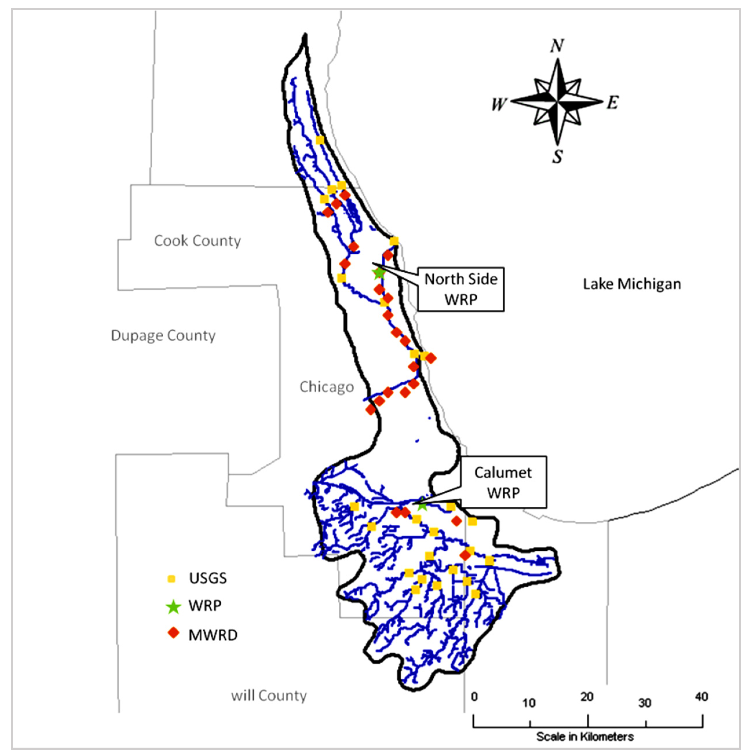
For this study, as part of building a framework for modeling the Chicago River Watershed, a data warehouse was created to aggregate available data from various agencies in the Chicago River Watershed. This helps to integrate the data for watershed assessment and physical modeling. Water quantity, water quality and land use data were compiled from different sources. The sources include U.S. Geologic Survey (USGS), Metropolitan Water Reclamation District of Greater Chicago (MWRD), Chicago Metropolitan Agency for Planning (CMAP), US Army Corps of Engineers—Chicago District (USACE), BASINS data store, and data from several facilities, treatment plants, and combined sewer overflows (CSOs) sources that are permitted through National Pollutant Discharge Elimination System (NPDES) permits. Figure 1 shows some of the data sources used in the model and their locations. There are 18 active USGS stations where water quantity data were obtained. They measure daily flow and gage heights in the watershed. Water quantity data were obtained from the MWRDGC available 41 stations within the watershed that measures up to 65 different water quality parameters monthly or bi-monthly. Land use inventory for 2001 and 2005 acquired from CMAP were utilized. Meteorological data comprised precipitation, air temperature, potential evapotranspiration, wind speed, solar radiation, dew point temperatures, and cloud cover were compiled from Chicago O’Hare Airport metrological station. Description of data sources are shown in Table 1.
3.2. Watershed Simulation
In the following subsections, steps to develop the water quality model to quantify the effect of detailed (level III) land use on nutrient loading in the Chicago River Watershed using BASINS/HSPF are outlined. It explains types and sources of data used and how hydrologic and water quality models were constructed and used in the BASINS/HSPF model environment.
BASINS provides different data layers to HSPF including: National Land Cover Data (NLCD or GIRAS) land use data to calculate land use distribution within watershed, meteorological data to provide meteorological data requirements, digital elevation model (DEM) grid data to determine boundaries of watershed, reach files to determine stream networks, permit compliance system (PCS) data to provide loading information in the watershed, and monitoring data such as STORET and USGS data to provide water quality and quantity data. Detailed land use data for the watershed, including 44 types of urban land use, were acquired from CMAP and added to BASINS. BASINS land use available are either Level (I) or Level (II) land use type. To fulfill the objective of the study level (III) land use type, CMAP’s 2005 land use inventory, in shapefile format, was added. The CMAP land shapefile was clipped into smaller shapefile to fit the watershed study area and because of limitations in processing detailed land use classifications in BASINS for larger area. To run HSPF, data was formatted to watershed data management (WDM) files that contain time series data required by HSPF. A user control input (UCI) file contains all the needed parameter values and control specifications to run the HSPF model. Calibration and validation analysis to evaluate the model are done using the GenScenario tool in the BASINS package. Delineation is a requirement process by HSPF and is either performed automatically using DEM grids or manually where existing streams and basins are manually selected and used to determine the watershed. The automatic delineation process used in this study ended up determining the streams, sub-basins, and outlets layers used in the simulation. The Upper Chicago River subbasin is divided into homogeneous land areas known as hydrologic response units (HRUs) that were used to define six reaches and seven subwatersheds. HRUs can be impervious or pervious areas, which, once determined, would be modeled independently. HSPF main simulation modules are PERLND, IMPLND, and RCHRES and they simulate pervious land segments, impervious land segments and free flow respectively [70]. The hydraulic characteristic of each reach was defined by parameters that represent volume–discharge relationships for each reach. Relationship between water level, surface area, volume and discharge are fixed. In order to simulate hydrology, sediments, and nutrients for each individual HRU, input data such as meteorological data and parameters related to land use, soil characteristics for each HRU are needed [70].
3.2.1. Impervious Area Assumptions
To determine the percentage of impervious area assigned for each HRU that represent the land use in the area, some estimation and consideration had to be made. The EIA as a percentage of TIA was determined for basins that are directly connected to the drainage systems [46]. TIA is determined using land use maps and aerial photography [71]. The majority of impervious surface studies correlate percentage of impervious surface to land use by using estimates of the proportion of imperviousness within each class. The TIA and EIA percentages and equations, based on the literature [45], used in this study are shown in Table 2 and Table 3, respectively.
3.2.2. Flow Simulation
The first component to be simulated in HSPF is the flow. IWATER and PWATER modules are used for the flow simulation. IWATER module simulates retention, routing, and evaporation of water from impervious segments. PWATER module computes the water budget and predicts the total runoff from pervious segments. The hydraulic behavior in the streams is simulated by the HYDR module. A fixed relationship is assumed among water level, surface area, volume, and discharge in each reach. In-stream simulation is assumed to be mixed-system with unidirectional and longitudinal flow simulation. The hydraulic characteristics of reaches are defined by parameters such as nominal upper zone storage, nominal lower zone storage, soil moisture infiltration rate, percent vegetation cover of each land use type, and groundwater recession rate. The parameters’ values were populated with BASINS default values and literature values and later adjusted during hydrologic calibration.
3.2.3. Water Quality Simulation
Water quality simulation in HSPF is done using IQUAL and PQUAL modules for impervious and pervious land segments respectively. Pollutants are simulated in the IQUAL and PQUAL modules using either direct washoff by overland flow where pollutant is simulated based on basic depletion and accumulation rate; or by washoff of detached sediments that are simulated as a function of sediment removal. The direct washoff by overland flow approach was adopted for all simulated constituents since the study area is largely impervious. Several biological, physical, and chemical processes within stream reaches are simulated in HSPF using the RCHRES module. The reaches are assumed to be completely mixed and the flow is unidirectional. Point sources added to the simulation are the two known NPDES in the watershed, which are North Side WRP and Calumet Water WRP. NPDES were included as direct inputs to the main reaches in the watershed. Pollutant species considered are the total nitrates as nitrogen (NO2 + NO3), total ammonia (NH3 + NH4+), and TP as phosphorus. For this study only the North shore WRP was considered as Calumet WRP was out of the scope of the study area.
3.2.4. Model Calibration and Validation
Models need to be evaluated to provide a quantitative estimate of performance and predictive ability of the model [72]. For HSPF evaluation, a weight of evidence approach that considers multiple graphical and statistical model comparisons, is commonly accepted and used to assess model performance [73]. The calibration–validation process is a hierarchal process where the parameters are first developed, then hydrology calibration–validation is done, and finally, water quality calibration–validation is performed. In this study Pearson’s correlation (r) and determination (r2) coefficients were used for evaluation. For model performance, r values range from −1 to 1 and for r2 values range from 0 to 1, a value >0.5 are considered acceptable [73]. A major drawback for r2 is its dispersion property, since systematically over- or under-predicted values still result in good r2 values. Another model evaluation criterion is the Nash–Sutcliffe efficiency coefficient (NSE). NSE lies between 1 (perfect fit) and −∞. The main disadvantage of NSE is that the differences between the observed and simulated values are calculated as squared values resulting in larger values being overestimated and lower values being neglected [72]. Other statistical indices used to evaluate the model performance in this study are root mean square error (RMSE), normalized root mean square error (NRMSE), and mean absolute error (MAE). RMSE and MAE measure the aggregated differences between simulated values and observed values where values close to zero indicate better model performance. The last evaluation index used in the study is the percent mean error (PME). PME is a general guidance measure that has been specifically used to evaluate the HSPF model performance [73]. It provides percent mean errors or differences between simulated and observed values, so that HSPF users can determine the level of agreement or accuracy (very good, good, and fair) that might be expected using the model [73]. PME target values for different modeling process [73] are shown in Table 4. Using all the above measures fulfilled the weight of evidence approach adopted in this study to evaluate the model.
4. Results and Discussion
4.1. Flow Calibration and Validation
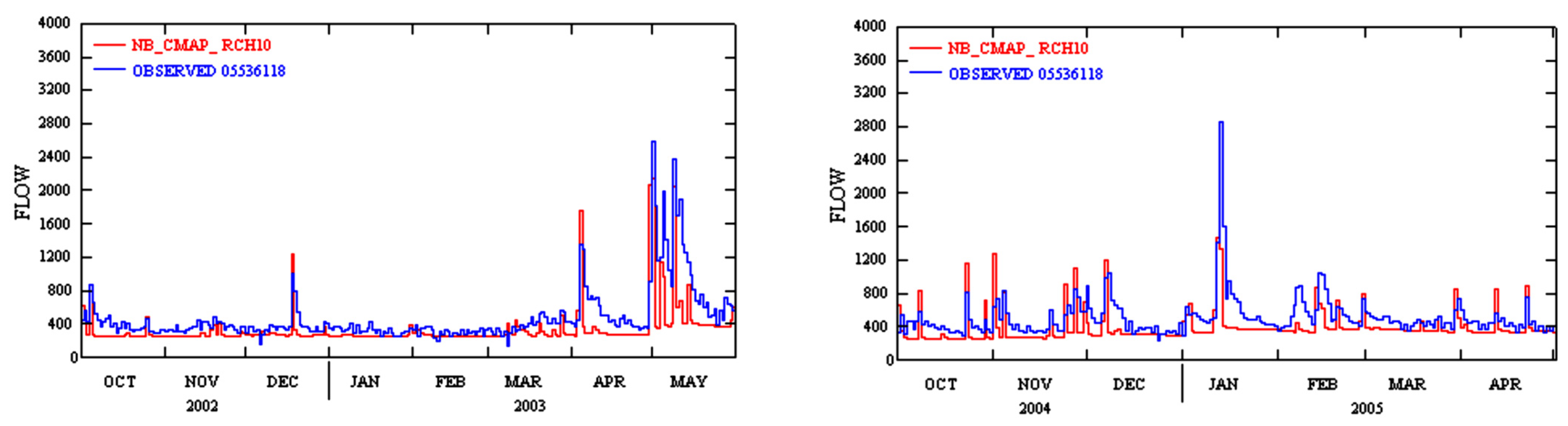
Meteorological data from Chicago O’Hare airport station was used to simulate the stream flow. To calibrate and measure flow sensitivity to impervious land segments, the EIA equations proposed by Alley, Laenen, and Sutherland [46,47,48] shown Table 3 were adopted. The percentages of pervious and impervious land segments were found accordingly. The calculated land uses were used in the flow simulation iterative procedure. Due to limited availability of data and input parameters for pervious and impervious land segments, BASINS’s default input parameters were initially applied. Parameters used were lower storage nominal (LZSN), upper zone storage nominal (UZSN), mean soil infiltration rate (INFILT), lower zone evapotranspiration (LZETP), ground water detention storage (INTFW), and interflow recession coefficient (IRC). These parameters are used for calibration and can be estimated and adjusted until calibration process is complete. LZSN, UZSN and INFILT are parameters that affect the total annual flow volume. LZETP, INTFW, and IRC are parameters that affect the base flow conditions of the river and hydrograph shape and peak flow conditions. The various module parameters were repeatedly adjusted and simulated and observed values were compared until reasonable r and r2 were obtained. Sensitivity analysis results for EIA equations for the study area are shown in Table 5. Lanen’s EIA equation (equation 4) showed acceptable performance and it was the one adopted for calculating EIA and determining percentages of pervious and impervious land segments for the watershed. For hydrology calibration and validation, the calibration period was October 2002 to May 2003 and the validation period was October 2004 to April 2005. The calibration and validation results for flow simulation are shown in Figure 2. The statistical indicators are fair based on graphical representation and according to the guidelines given by Donigian [73]. The model showed better performance in the validation period relative to the calibration period except for the poor r and fair to acceptable r2. According to Table 6, the model’s performance is considered acceptable based on statistical indicators and acceptable ranges published in the literature for hydrologic simulation given the collective criteria measure.
4.2. Water Quality Calibration and Validation
The calibration and validation process in HSPF model is a hierarchical process that starts with the hydrology and ends with water quality constituents [73]. Constituents simulated were total ammonium (NH3 + NH4) as N, total nitrate (NO3 + NO2) as N, and ortho phosphorus (PO4). Total nitrogen and phosphorous loads were later calculated utilizing scripts provided in the model. Several nutrient parameters were added in the model for both pervious and impervious land segments including initial storage for each constituent, constituent washoff factor, and monthly constituent accumulation factor. These parameters were adjusted and calibrated until reasonable model behavior was seen.
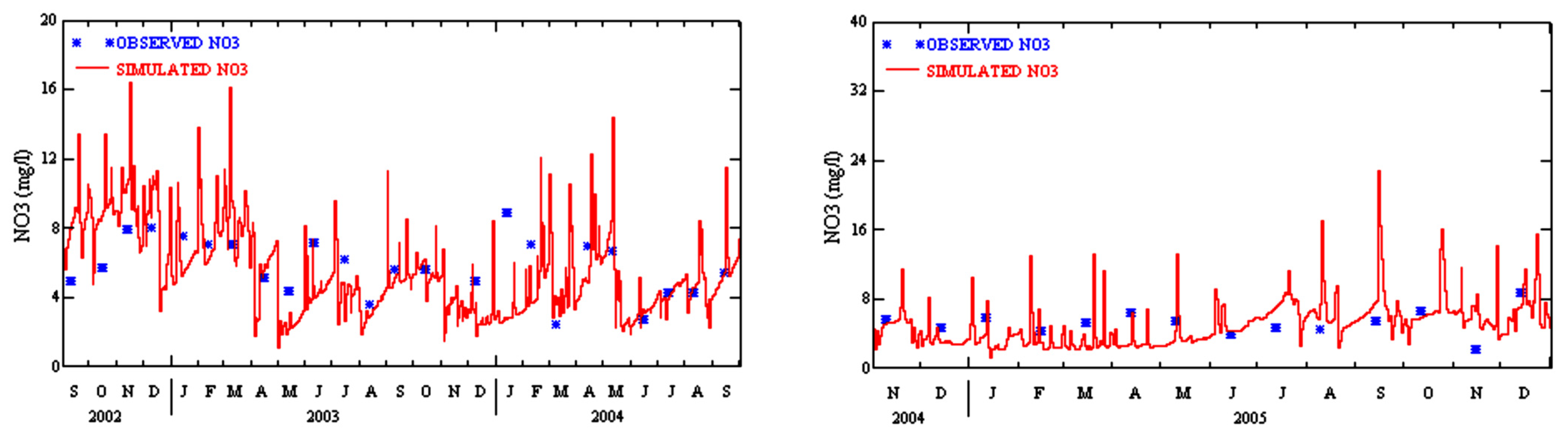
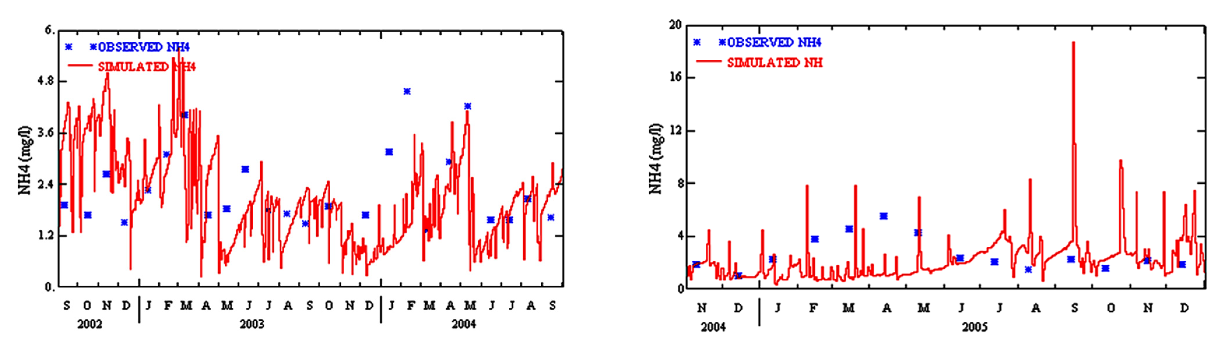
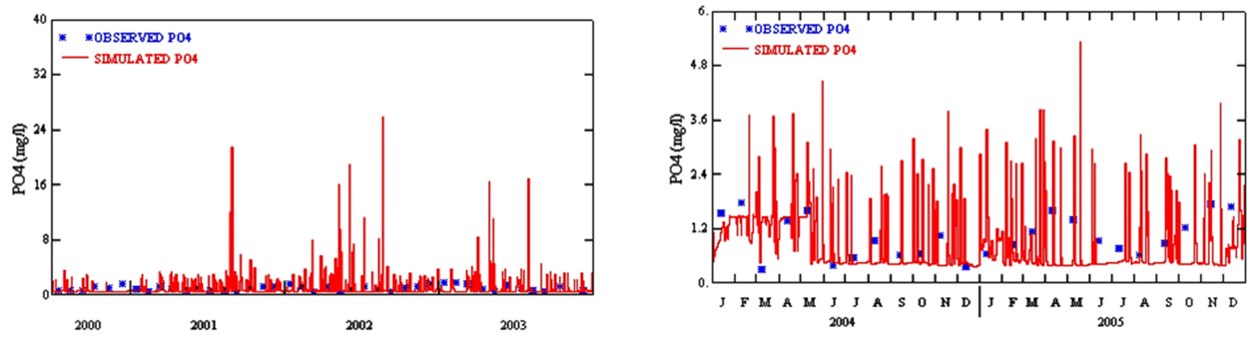
The simulation results were compared to observed values at the North Branch of the Chicago River monitoring station at Grand Ave, Chicago. The location was chosen to represent the outlet for the sub-basin. Two factors limited the time period for the calibration and validation of the model used for the water quality simulation. The observed flow at the monitoring station was limited to the period 2002–2010 (with some missing data in the period 2003–2004), while the meteorological data was only available for the period 2002–2006. The initial simulation values were consistently over predicted, mostly during the wet season. To address this, calibration parameters—including the monthly accumulation factors and monthly values for limiting storage for both pervious and impervious land segments—were repeatedly adjusted. The instream simulation process parameters, nitrification and denitrification parameters (KNO320), along with oxidation rate (KTAM20) and algal growth rate parameters were all adjusted until reasonable modeling results were obtained. The calibration and validation results for total nitrates, total ammonium and ortho phosphate simulation are shown in Figure 3, Figure 4 and Figure 5. Table 7 summarizes the water quality calibration and validation statistical for the simulated nutrients. Calibration results show that there is an acceptable agreement between the observed and simulated data. Statistical results and model performance are considered good to very good for all the constituents as it fell within the accepted tolerances suggested by Donigian (Table 4).
4.3. Total Annual Loads of Nutrients
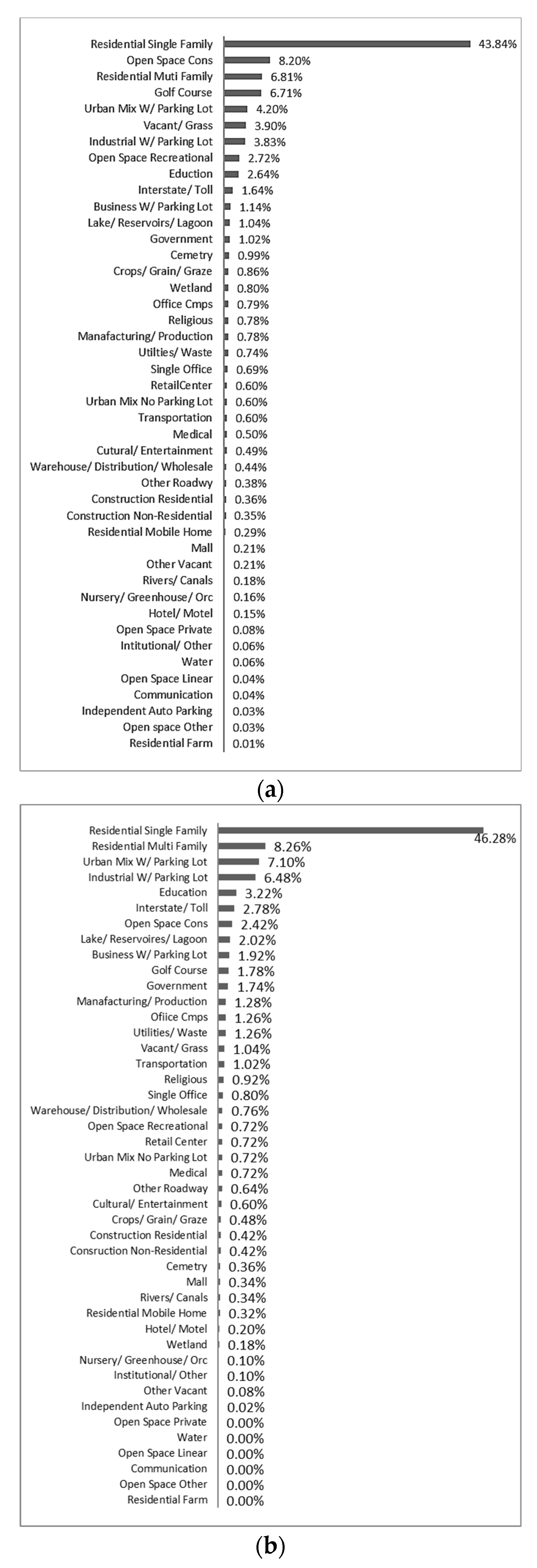
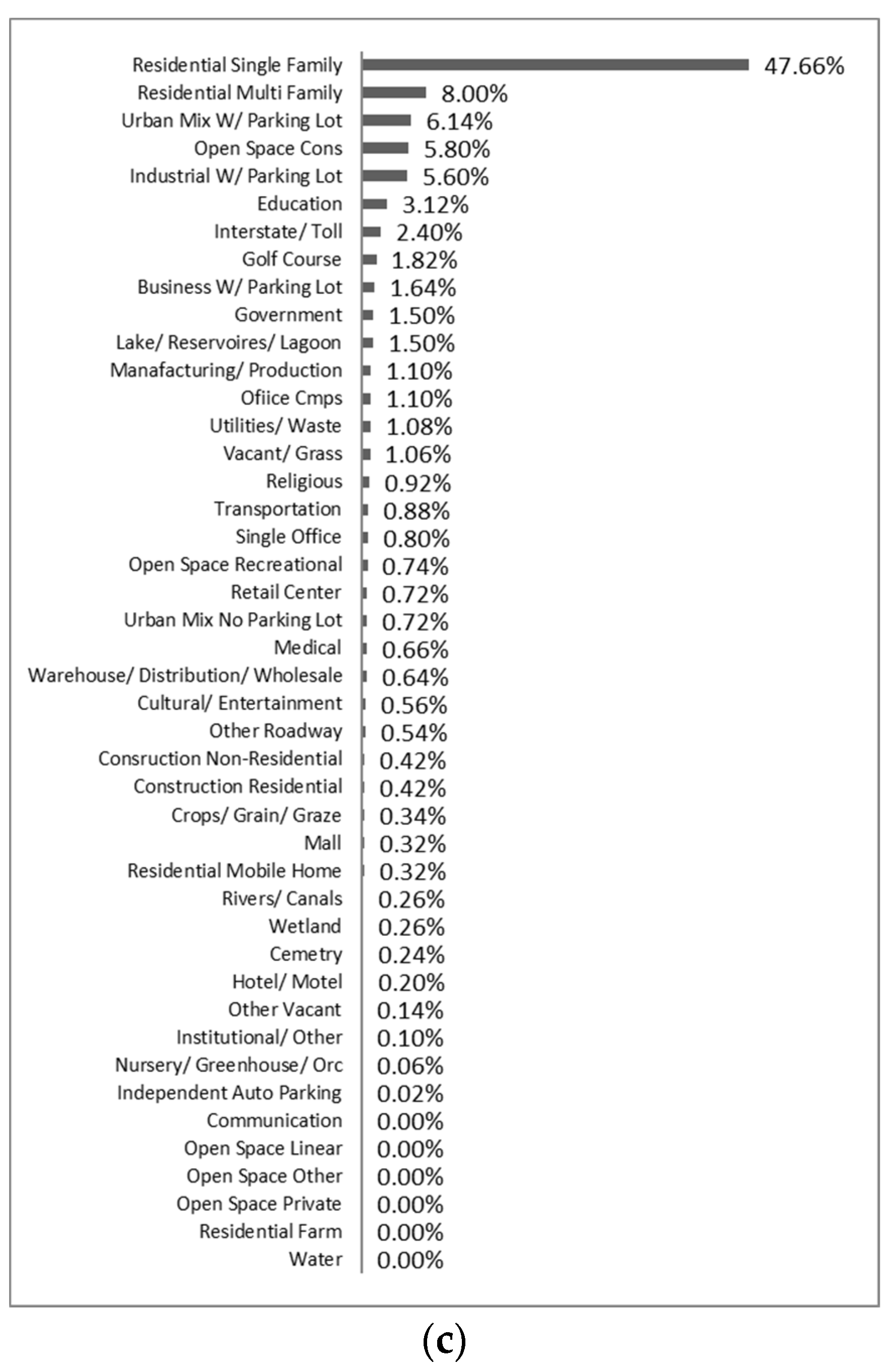
Different studies have done significant progress, using long term modeling and machine learning, towards estimating inputs of total nitrogen and total phosphorus loads to receiving waters in metropolitan areas [74,75]. However, there have been fewer studies that explore the long-term hydrological conditions and detailed land use in the context of high urbanized watershed. For this study, HSPF modules PQUAL and IQUAL were used to estimate annual loadings of total nitrogen and total phosphorus from forty-four different land use types in the Upper Chicago River Basin. Based on the results from the calibrated and validated water quality model, the total annual loads from the Upper North Chicago River sub-basin were computed using scripts provided by HSPF that transfer simulated total nitrates and total ammonium into total nitrogen loads and simulated ortho phosphate into total phosphorus loads. To compare different land use areas, total nitrogen and total phosphorous associated with each land use type percentage values are shown in Figure 6. The simulation results show that the highest total nitrogen and total phosphorus loads produced during the period of 2000 to 2005 in the Upper Chicago River sub-basin was for residential single-family land use. This is an expected result since residential single-family land use is the dominant land use type in the basin, as shown in Figure 6a. It was difficult to determine the accuracy of the loads simulated by this since no information available that can relate the contribution of a detailed land use, level (III), to the total nitrogen and total phosphorus loads to the Chicago River Watershed or any similar highly urbanized watersheds. However, based on the results of water quality model calibration and validation, it can be assumed that this a unique work in estimating total nitrogen and total phosphorus loads from a detailed land use segments in the watershed.
4.4. Export Coefficients of Detailed Land Uses
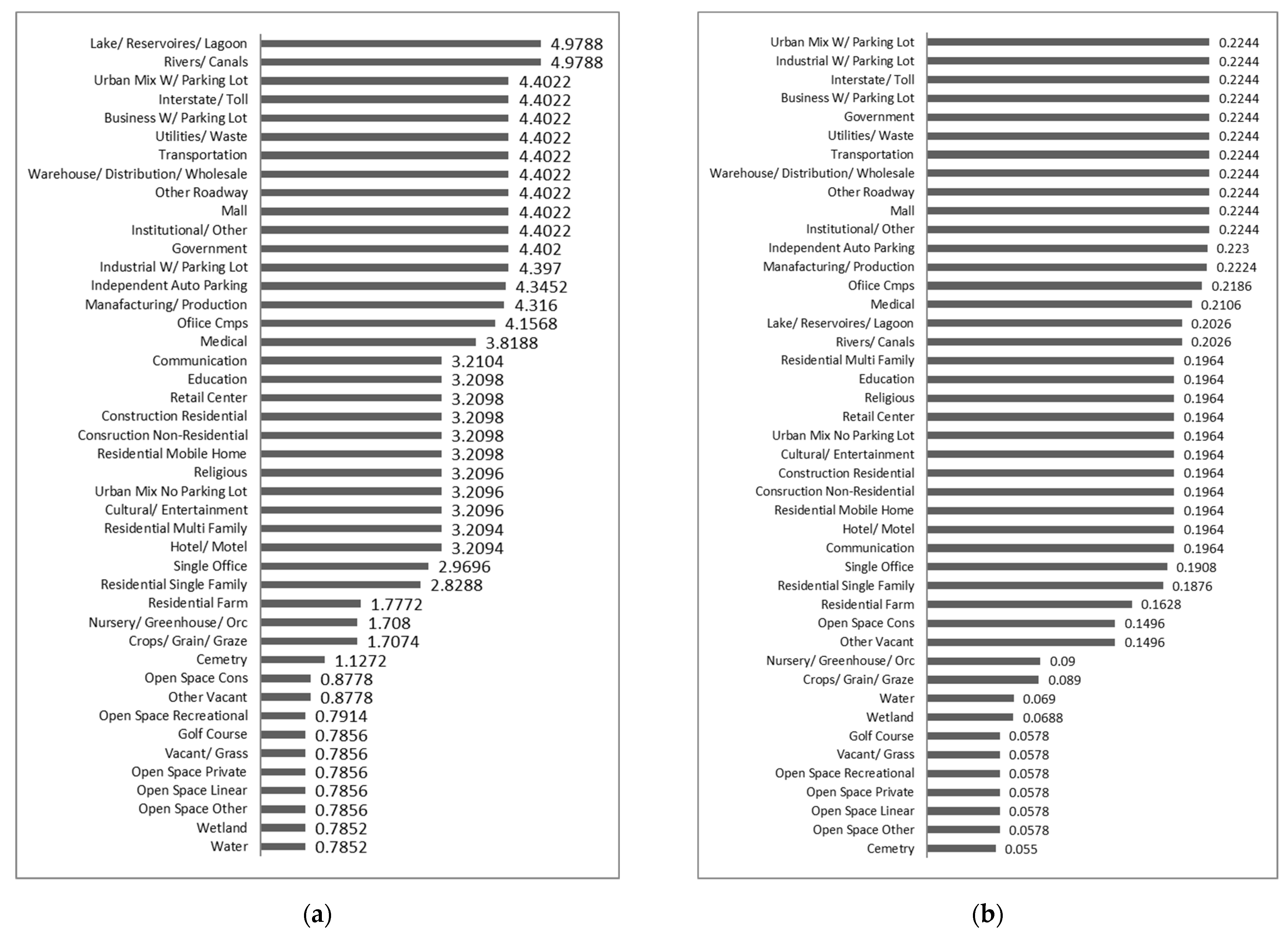
It is essential to adopt approaches to estimate different region-specific nutrient export coefficients other than the ones available in literature [74]. Although the literature is showing limited ranges of EC values for general land uses, the ranges of EC values presented in this section were found comparable with ranges established in literature [45,58,76]. The export coefficients presented in this study are believed to be the first attempt to measure and model TN and TP using detailed land use types in the Chicago River Watershed or any similar highly urbanized watersheds using a continuous simulation approach and watershed perspective analysis. ECs are very useful indicators that allow the prediction of the possible yield of nutrients reaching receiving water bodies. The average obtained export coefficients for total nitrogen and total phosphorous, respectively, for each land use type investigated in this study are shown in Figure 7.
5. Conclusions
Simulation models at the watershed scale offer an effective watershed management tools to estimate nutrients yields for a wide spectrum of problems dealing with surface waters. Since the Chicago River Watershed is 82% urban land use (i.e., highly urbanized area), examining effect of land use on water quality requires a detailed level of land use. The five years of water quality simulation done using BASINS, coupled with the continuous simulation watershed scale model HSPF, resulted in unique export coefficients for level (III) detailed land use for the Chicago River Watershed. This can be considered as a successful contribution to measure and model nutrients in the watershed and allow the prediction of the possible yield of nutrients reaching receiving water bodies. This can provide a planning tool for regulatory environmental agencies in the Chicago River Watershed to develop better management programs especially if total maximum daily loads (TMDL) and water quality standards (WQS) are developed for the Chicago River Watershed. The model can be utilized in the investigation and analysis of future scenarios in the watershed. The range of land use export coefficients obtained from long term continuous simulation reflects the different conditions of watershed and different meteorological and physical variables included in the simulation and hence provide a perfect input for a multi-objective optimization approach to evaluate multiple scenarios that seek to find optimal land use change and distribution in highly urbanized developed watershed. Based on different detailed land use types, scenarios that take into account different combinations of pervious and impervious land use segments and tradeoffs between them (e.g., changing an impervious parking lot land use into pervious, etc.), along with factors such as environmental, social, and economical factors can be investigated as part of planning and decision-making tool. The multi-objective optimization approach will allow the optimizing of independent objectives to find the best land use combination while the high priority goal is to meet certain water quality standards regarding nutrient loadings of total nitrogen (TN) and total phosphorus (TP). The model can be successfully applied to any highly urbanized watershed with appropriate consideration given to EIA.
Author Contributions
Conceptualization, N.M. and K.R.P.; Data curation, N.M.; Formal analysis, N.M.; Methodology, N.M. and K.R.P.; Supervision, K.R.P.; Writing—original draft, N.M.; Writing—review and editing, N.M. and K.R.P. All authors have read and agreed to the published version of the manuscript.
Funding
This research received no external funding.
Institutional Review Board Statement
No human subjects were involved in this research.
Informed Consent Statement
Not applicable.
Data Availability Statement
The data presented in this study are available on request from the corresponding author.
Conflicts of Interest
The authors declare no conflict of interest.
References
- Tong, S.T.Y.; Liua, A.J.; Goodrich, J.A. Assessing the water quality impacts of future land-use changes in an urbanizing watershed. Civ. Eng. Environ. Syst. 2009, 26, 3–18. [Google Scholar] [CrossRef]
- Ren, W.W.; Zhong, Y.; Meligrana, J.; Anderson, B.; Watt, W.E.; Chen, J.K.; Leung, H.L. Urbanization, land use, and water quality in Shanghai 1947–1996. Environ. Int. 2003, 29, 649–659. [Google Scholar] [CrossRef]
- Tong, S.T.Y.; Chen, W. Modeling the relationship between land use and surface water quality. J. Environ. Manag. 2002, 66, 377–393. [Google Scholar] [CrossRef] [PubMed]
- Weng, Q. Modeling urban growth effects on surface runoff with the integration of remote sensing and GIS. Environ. Management 2001, 28, 737–748. [Google Scholar] [CrossRef] [PubMed]
- Bian, B.; Juan Cheng, X.; Li, L. Investigation of urban water quality using simulated rainfall in a medium size city of China. Environ. Monit. Assess. 2011, 183, 217–229. [Google Scholar] [CrossRef] [PubMed]
- Brezonik, P.L.; Stadelmann, T.H. Analysis and predictive models of storm water runoff volumes, loads, and pollution concentration from watersheds in the Twins Cities metropolitan area, Minnesota, USA. Water Res. 2002, 36, 1743–1757. [Google Scholar] [CrossRef]
- Zhu, W.; Bian, B.; Li, L. Heavy metal contamination of road-deposited sediments in a medium size city of China. Environ. Monit. Assess. 2008, 147, 171–181. [Google Scholar] [CrossRef] [PubMed]
- Malinowski, Ł.; Skoczko, I. Impacts of Climate Change on Hydrological Regime and Water Resources Management of the Narew River in Poland. J. Ecol. Eng. 2018, 19, 167–175. [Google Scholar] [CrossRef]
- Bhaduri, B.; Minner, M.; Tatalovich, S.; Harbor, J. Long-term hydrologic impact of land use change: A tale of two models. J. Water Resour. Plan. Manag. 2001, 127, 13–19. [Google Scholar] [CrossRef]
- Bhaduri, B.; Harbor, J.; Engel, B.A.; Grove, M. Assessing watershed-scale, long-term hydrologic impacts of land-use change using a GIS-NPS model. Environ. Manag. 2000, 26, 643–658. [Google Scholar] [CrossRef]
- Erickson, J.J.; Smith, C.D.; Goodridge, A.; Nelson, K.L. Water quality effects of intermittent water supply in Arraiján, Panama. Water Res. 2017, 114, 338–350. [Google Scholar] [CrossRef] [PubMed]
- Piazza, S.; Sambito, M.; Feo, R.; Freni, G.; Puleo, V. CCWI2017: F6 ’Optimal positioning of water quality sensors in water distribution networks: Comparison of numerical and experimental results. Univ. Sheffield. J. Contribution 2017. [Google Scholar] [CrossRef]
- Hepinstall, J.A.; Alberti, M.; Marzluff, J.M. Predicting land cover change and avian community response in rapidly urbanizing environments. Landscape Ecology 2008, 23, 1257–1276. [Google Scholar] [CrossRef]
- Feddema, J.J.; Oleson, K.W.; Bonan, G.B.; Mearns, L.O.; Buja, L.E.; Meehl, G.A.; Washington, W.M. The importance of land-cover changes in simulating future climates. Science 2005, 310, 1674–1678. [Google Scholar] [CrossRef] [PubMed] [Green Version]
- Foley, J.A.; Defies, R.; Asner, G.P.; Barford, C.; Bonan, G.; Carpenter, S.R. Global Consequences of Land Use. Science 2005, 309, 5734. [Google Scholar] [CrossRef] [Green Version]
- Ahearn, D.S.; Sheibley, R.W.; Dahlgren, R.A.; Anderson, M.; Johnson, J.; Tate, K.W. Land use and land cover influence on water quality in the last free-owing river draining the western Sierra Nevada, California. J. Hydrol. 2005, 313, 234247. [Google Scholar] [CrossRef]
- Brett, M.T.; Arhonditsis, G.B.; Mueller, S.E.; Hartley, D.M.; Frodge, J.D.; Funke, D.E. Nonpoint source impacts on stream nutrient concentrations along a forest to urban gradient. Environ. Manag. 2005, 35, 330–342. [Google Scholar] [CrossRef]
- Rose, S.; Peters, N.E. Effects of urbanization on streamflow in the Atlanta area (Georgia, USA): A comparative hydrological approach. Hydrol. Process. 2001, 15, 1441–1457. [Google Scholar] [CrossRef]
- Paul, M.J.; Meyer, J.L. Streams in the urban landscape. Annual Rev. Ecol. Syst. 2001, 32, 333–365. [Google Scholar] [CrossRef]
- Schueler, T.R. The importance of imperviousness. Pract. Watershed Prot. 2000, 1, 7–18. [Google Scholar]
- Cianfrani, C.M.; Hession, W.C.; Rizzo, D.M. Watershed imperviousness impacts on stream channel condition in South Eastern Pennsylvania. J. Am. Water Resour. Assoc. 2006, 42, 941–956. [Google Scholar] [CrossRef]
- Tsegaye, T.; Sheppard, D.; Islam, K.R.; Johnson, A.; Tadesse, W.; Atalay, A.; Marzen, L. Development of chemical index as a measure of in-stream water quality in response to landuse and land cover changes. Water Air Soil Pollut. 2006, 174, 161–179. [Google Scholar] [CrossRef]
- Tang, Z.; Engel, B.A.; Pijanowski, B.C.; Lim, K.J. Forecasting land use change and its environmental impact at a watershed scale. J. Environ. Manag. 2005, 76, 35–45. [Google Scholar] [CrossRef]
- Maestas, J.D.; Knight, R.L.; Gilgert, W. Biodiversity Across a Rural Land Use Gradient. Conserv. Biol. 2003, 17, 1425–1434. [Google Scholar] [CrossRef] [Green Version]
- Loomis, J. Integrated Public Lands Management: Principles and Applications to National Forests, Parks, Wildlife Refuges, and BLM Lands; Columbia University Press: New York, NY, USA, 2002. [Google Scholar]
- Wu, Q.; Li, H.; Wang, R.; Paulussen, J.; He, Y.; Wang, M. Monitoring and predicting land use change in Beijing using remote sensing and GIS. Landsc. Urban. Plan. 2006, 78, 322–333. [Google Scholar] [CrossRef]
- Conway, T.M.; Lathrop, L.G. Alternative land use regulations and environmental impacts: Assessing future land use in an urbanizing watershed. Landsc. Urban. Plan. 2005, 70, 1–15. [Google Scholar] [CrossRef]
- Wang, S.H.; Huggins, D.G.; Frees, L.; Volkman, C.G.; Lim, N.C.; Baker, D.S.; Smith, V.; Denoyelles, F. An integrated modeling approach to total watershed management: Water quality and watershed management of Cheney Reservoir. Water Air Soil Pollut. 2005, 164, 1–19. [Google Scholar] [CrossRef]
- Zoppou, C. Review of urban storm water models. Environ. Model. Softw. 2001, 16, 195231. [Google Scholar] [CrossRef]
- Tong, S.T.Y.; Liu, A.J.; Goodrich, J.A. Climate change impacts on nutrient and sediment loads in a Midwestern agricultural watershed. J. Environ. Inform. 2007, 9, 18–28. [Google Scholar] [CrossRef]
- Wilson, C.O.; Weng, Q. Simulating the impacts of future land use and climate changes on surface water quality in the Des Plaines River watershed, Chicago Metropolitan Statistical Area, Illinois. Sci. Total. Environ. 2011, 409, 4387–4405. [Google Scholar] [CrossRef] [PubMed]
- Akhavan, S.; Abedi-Koupai, J.; Mousavi, S.-F.; Afyuni, M.; Eslamian, S.S.; Abbaspour, K.C. Application of SWAT model to investigate nitrate leaching in Hamadan-Bahar Watershed, Iran. Agriculture. Ecosyst. Environ. 2010, 139, 675–688. [Google Scholar] [CrossRef]
- Allan, J.D. Landscapes and Riverscapes: The influence of land use on stream ecosystems. Annu. Rev. Ecol. Evol. Syst. 2004, 35, 257–284. [Google Scholar] [CrossRef] [Green Version]
- Leon, L.F.; Booty, W.; Wong, I.; McCrimmon, C.; Melles, S.; Benoy, G.; Vanrobaeys, J. Advances in the integration of watershed and lake modeling in the Lake Winnipeg basin. Modelling for Environment’s Sake. In Proceedings of the 5th Biennial Conference of the International Environmental Modelling and Software Society, Ottawa, ON, Canada, 4–8 July 2010; pp. 860–867. [Google Scholar]
- Tong, S.T.Y.; Liu, A.J. Modelling the hydrologic effects of land-use and climate changes. Int. J. Risk Assess. Manag. 2006, 6, 344–368. [Google Scholar] [CrossRef]
- Nu-Fang, F.; Zhi-Hua, S.; Lu, L.; Cheng, J. Rainfall, runoff, and suspended sediment delivery relationships in a small agricultural watershed of the Three Gorges area, China. Geomorphology 2011, 135, 158–166. [Google Scholar] [CrossRef]
- Sheng, Y.; Ying, G.; Sansalone Sheng, J. Differentiation of transport for particulate and dissolved water chemistry load indices in rainfall–runoff from\urban source area watersheds. J. Hydrol. 2008, 361, 144–158. [Google Scholar] [CrossRef]
- Najafi, M.Z. Watershed modeling of rainfall excess transformation into runoff. J. Hydrol. 2003, 270, 273–281. [Google Scholar] [CrossRef]
- Muzik, I. A first-order analysis of the climate change effect on flood frequencies in a subalpine watershed by means of a hydrological rainfall–runoff model. J. Hydrol. 2002, 267, 65–73. [Google Scholar] [CrossRef]
- Singh R, K.; Panda, R.K.; Satapathy, K.K.; Ngachany, S.V. Simulation of runoff and sediment yield from a hilly watershed in the eastern Himalaya, India using the WEPP model. J. Hydrol. 2011, 405, 261–276. [Google Scholar] [CrossRef]
- Yu, X.; Zhang, X.; Niu, L. Simulated multi-scale watershed runoff and sediment production based on GeoWEPP model. Int. J. Sediment. Res. 2009, 24, 465–478. [Google Scholar] [CrossRef]
- Jeon, J.; Yoon, C.G.; Donigian, A.S., Jr.; Jung, W. Development of the HSPF Paddy model to estimate watershed pollutant loads in paddy farming regions. Agric. Water Manag. 2007, 90, 75–86. [Google Scholar] [CrossRef]
- Jacobson, C.R. Identification and quantification of the hydrological impacts of imperviousness in urban catchments: A review. J. Environ. Manag. 2011, 92, 1438–1448. [Google Scholar] [CrossRef] [PubMed]
- Smith, T.E.; Deacon, J.R.; Soule, S.A. Effects of urbanization on stream quality at selected sites in the Seacoast region in New Hampshire. U.S. Geol. Surv. Sci. Investig. Rep. 2005, 5103, 18. [Google Scholar]
- Brabec, E.; Schulte, S.; Richards, P.L. Impervious surfaces and water quality: A review of current literature and its implications for watershed planning. J. Plan. Lit. 2002, 16, 499. [Google Scholar] [CrossRef]
- Sutherland, R.C. Methods for estimating the effective impervious area of urban watersheds. Pract. Watershed Prot. 2000, 32, 193–195. [Google Scholar]
- Alley, W.M.; Veenhuis, J.E. Effective impervious area in urban runoff modeling. J. Hydraul. Eng. 1983, 109, 313–319. [Google Scholar] [CrossRef]
- Laenen, A. Storm Runoff as Related to Urbanization based on Data Collected in Salem and Portland, and Generalized for the Willamette Valley, Oregon. U.S. Geological Survey Water Resources Investigations Report 83-4143. Available online: http://or.water.usgs.gov/pubs_dir/orrpts.html (accessed on 21 November 2011).
- Luzio, M.D.; Srinivian, R.; Arnold, J.G. Integration of watershed tools and swat model to basins. J. Am. Water Resour. Assoc. 2002, 38, 1127–1142. [Google Scholar] [CrossRef]
- Fohrer, N.; Haverkamp, S.; Eckhardt, K.; Frede, H.G. Hydrologic response to land use changes on the catchment scale. Phys. Chem. Earth 2001, 26, 577–582. [Google Scholar] [CrossRef]
- Wicklein, S.M.; Schiffer, D.M. Simulation of Runoff and Water Quality for 1990 and 2008 Land-Use Conditions in the Reedy Creek Watershed, East-Central Florida. Water-Resources Investigations Report 02-4018; U.S. Geological Survey. 2008. Available online: http://pubs.usgs.gov/wri/ (accessed on 2 May 2012).
- Shirinian, O.; Anne, A.; Christopher G., U. Modeling the Hydrology and water quality using BASINS/HSPF for the upper Maurice River watershed, New Jersey. J. Environ. Sci. Health J. Environ. Sci. Health Part A Toxic/Hazard. Subst. Environ. Eng. 2007, 42, 289–303. [Google Scholar]
- Singh, V.P.; Frevert, D.K. Watershed Modeling. ASCE Conf. Proc. 2003, 1–37. [Google Scholar] [CrossRef]
- Im, S.; Brannan, K.M.; Mostaghimi, S. Simulating hydrologic and water quality impacts in an urbanizing watershed. J. Am. Water Resour. Assoc. 2003, 39, 1465–1479. [Google Scholar] [CrossRef]
- Brun, S.E.; Band, L.E. Simulating runoff behavior in an urbanizing watershed. Computers. Environ. Urban. Syst. 2000, 24, 5–22. [Google Scholar] [CrossRef]
- Mohamoud, Y.M.; Parmar, R.; Wolfe, K. Modeling Best Management Practices (BMPs) with HSPF. Modeling Best Management Practices (BMPs) with HSPF. Proceeding of Watershed Management Conference 2010: Innovations in Watershed Management under Land Use and Climate Change, Madison, Wisconsin, 23–27 August 2010. [Google Scholar] [CrossRef]
- Bergman, M.J.; Green, W.; Donnangelo, L.J. Calibration of storm loads in the South Prong watershed, Florida, using Basins/HSPF. J. Am. Water Res. Assoc. 2002, 38, 1423–1436. [Google Scholar] [CrossRef]
- Lin, J. Review of Published Export Coefficient and Event mean Concentration Data. US Army Corps of Engineer, Wetlands Regulatory Assistance Program. ERDC TN-WRAP-04-3: 2004. Available online: http://el.erdc.usace.army.mil/elpubs/pdf/tnwrap04-3.pdf (accessed on 16 October 2011).
- Mcfarland, A.M.S.; Hauck, L.M. Determining nutrient export coefficients and source loading uncertainty using in stream monitoring data. J. Am. Water Resour. Assoc. 2001, 37, 223–236. [Google Scholar] [CrossRef]
- Line, D.E.; White, N.M.; Osmond, D.L.; Jennings, G.D.; Mojonnier, C.B. Pollutant export from various land uses in the Upper Neuse River Basin. Water Environ. Res. 2002, 74, 100–108. [Google Scholar] [CrossRef] [PubMed]
- Quijano, J.C.; Zhu, Z.; Morales, V.; Landry, B.J.; Garcia, M.H. Three-dimensional model to capture the fate and transport of combined sewer overflow discharges: A case study in the Chicago Area Waterway System. Sci. Total. Environ. 2017, 576, 362–373. [Google Scholar] [CrossRef] [PubMed]
- Bartosova, A.; Singh, J.; Rahim, M.; McConkey, S. Phase II: Hydrologic and water quality simulation models, part 3: Validation of hydrologic model parameters, Brewster Creek, Ferson Creek, Flint Creek, Mill Creek, and Tyler Creek Watersheds. In Fox River Watershed Investigation: Stratton Dam to the Illinois River; ISWS CR 2007-07; Illinois State Water Survey, Center for Watershed Science: Champaign, IL, USA, 2007. [Google Scholar]
- Demissie, M.; Singh, J.; Knapp, H.V.; Saco, P.; Lian, Y. Hydrologic Model Development for the Illinois River Basin Using BASINS 3.0; ISWS CR 2007-03; Illinois State Water Survey, Center for Watershed Science: Champaign, IL, USA, 2007. [Google Scholar]
- Bartosova, A.; Singh, J.; Slowikowski, J.; Machesky, M.; McConkey, S. Overview of Recommended Phase III Water Quality Monitoring: Fox River investigation; ISWS CR 2005-13; Illinois State Water Survey, Center for Watershed Science: Champaign, IL, USA, 2005. [Google Scholar]
- Knapp, H.V.; Singh, J.; Andrew, K. Hydrologic Modeling of Climate Scenarios for Two Illinois Watersheds; ISWS CR 2004-07; Illinois State Water Survey, Center for Watershed Science: Champaign, IL, USA, 2004. [Google Scholar]
- Singh, J.; Knapp, H.V.; Demissie, M. Hydrologic Modeling of the Iroquois River Watershed Using HSPF and SWAT; ISWS CR 2004-08; Illinois State Water Survey, Center for Watershed Science: Champaign, IL, USA, 2004. [Google Scholar]
- U.S. Geological Survey. Environmental Setting of the Upper Illinois River Basin and Implications for Water Quality; Water-Resources Investigations Report 98–4268; U.S. Geological Survey (USGS): Urbana, IL, USA, 1999.
- CMAP. Chicago Metropolitan Agency for Planning. 2021. Available online: https://www.cmap.illinois.gov/data/land-use/inventory (accessed on 15 August 2021).
- Metropolitan Water Reclamation District of Greater Chicago. Cook County Stormwater Management Plan. Metropolitan Water Reclamation District of Greater Chicago. 2007. Available online: http://www.mwrd.org/ (accessed on 18 June 2011).
- Donigian, A.S.; Bicknell, B.R.; Imhoff, J.C. Hydrological Simulation Program Fortran (HSPF). In Computer Models of Watershed Hydrology; Chapter 12; Sigh, V.P., Ed.; Water Resources Publications: Littleton, CO, USA, 1995; pp. 395–442. [Google Scholar]
- Jones, T.; Johnston, C.; Kipkie, C. Using annual hydrographs to determine effective impervious area. Pract. Modeling Urban. Water Syst. 2003, 11, 291–306. [Google Scholar] [CrossRef]
- Krause, P.; Boyle, D.; Base, F. Comparison of different efficiency criteria for hydrological model assessment. Adv. Geosci. 2005, 5, 89–97. [Google Scholar] [CrossRef] [Green Version]
- Donigian, A.S. HSPF Watershed Model Calibration and Validation; Aquaterra Consultants: Mountain View, CA, USA, 2002. [Google Scholar]
- Han, B.; Reidy, A.; Li, A. Modeling nutrient release with compiled data in a typical Midwest watershed. Ecol. Indic. 2021, 121, 107213, ISSN 1470-160X. [Google Scholar] [CrossRef]
- Shen, L.Q.; Amatulli, G.; Sethi, T. Estimating nitrogen and phosphorus concentrations in streams and rivers, within a machine learning framework. Sci. Data 2020, 7, 161. [Google Scholar] [CrossRef] [PubMed]
- White, M.; Harmel, D.; Yen, H.; Arnold, J.; Gambone, M.; Haney, R. Development of Sediment and Nutrient Export Coefficients for U.S. Ecoregions 2015, 51, 758–775. [Google Scholar] [CrossRef]
Figure 1.
Data sources and locations used in the model.

Figure 2.
Flow calibration and validation.

Figure 3.
Total nitrates calibration and validation.

Figure 4.
Total ammonium calibration and validation.

Figure 5.
Ortho phosphate calibration and validation.

Figure 6.
Percentages of (a) land use area, (b) total nitrogen loads, and (c) total phosphorous loads in the Upper Chicago River Basin.
Figure 6.
Percentages of (a) land use area, (b) total nitrogen loads, and (c) total phosphorous loads in the Upper Chicago River Basin.


Figure 7.
Average EC for (a) total nitrogen and (b) total phosphorous (lbs/acre/yr.).


Table 1.
Description of data sources used in the model.
| Source | Data Type | Years |
|---|---|---|
| USGS | Daily discharge, daily gage heights | 1970–2010 |
| MWRDGC | Daily WRP effluents, monthly and bi-monthly water quality parameters, NPDES, CSOs | 1970–2008 |
| CMAP | Land use Inventory | 2001, 2005 |
| USACE | Daily and hourly precipitation | 1999–2006 |
| BASINS | Hourly meteorological data | 1970–2006 |
Table 2.
Examples of TIA percentages used in this study.
| Land Use Class | (TIA)% |
|---|---|
| Multi-Family Residential | 50 |
| Single-Family Residential | 35 |
| Commercial | 85 |
| Industrial | 85 |
| Roads | 85 |
| Schools | 50 |
| Public Open Space | 0 |
| Agricultural | 0 |
| Forest | 0 |
| Vacant | 0 |
| Water | 100 |
Table 3.
EIA equations used in this study.
| Source | EIA Equation |
|---|---|
| Sutherland (Totally connected) | (TIA) |
| Sutherland (Highly connected) | (0.4 × TIA1.2) |
| Alley et al. | (0.15 × TIA1.41) |
| Laenen | (3.6 + 0.43 × TIA) |
Table 4.
PME calibration and validation target values for HSPF.
| Very Good | Good | Fair | |
|---|---|---|---|
| Hydrology/Flow | <10 | 10–15 | 15–25 |
| Water Quality/Nutrients | <15 | 15–25 | 25–35 |
| Sediment | <20 | 20–30 | 30–45 |
| Pesticides/Toxics | <20 | 20–30 | 30–40 |
Table 5.
Sensitivity analysis for EIA equations.
| EIA Equation | r | r2 |
|---|---|---|
| 1 Sutherland, Totally connected basins, | 0.67 | 0.41 |
| (EIA = TIA) | ||
| 2 Sutherland, Highly connected basins, | 0.67 | 0.45 |
| (EIA = 0.4 × TIA1.2) | ||
| 3 Alley et al., (EIA = 0.15 × TIA1.41) | 0.67 | 0.45 |
| 4 Lanen, (EIA = 3.6 + 0.43 × TIA) | 0.71 | 0.51 |
Table 6.
Flow calibration and validation statistical results.
| Observed Mean Flow (ft³/s) | Simulated Mean Flow (ft³/s) | PME | r | r2 | NSE | RMSE | NRMS | |
|---|---|---|---|---|---|---|---|---|
| Calibration | 470.13 | 335.30 | 28.6 | 0.71 | 0.51 | −0.16 | 0.76 | 0.06 |
| Validation | 484.18 | 358.33 | 25.9 | 0.37 | 0.61 | −0.10 | 0.38 | 0.04 |
Table 7.
Water quality calibration and validation statistical results.
| Constituents | Mean Observed (mg/L) | Mean Simulated (mg/L) | ME | PME | MAE | RMSE | NSE | |
|---|---|---|---|---|---|---|---|---|
| Calibration | Nitrate-N | 5.81 | 5.50 | 0.228 | 3.93 | 1.74 | 2.21 | 0.13 |
| Ammonia-N | 2.29 | 2.09 | 0.048 | 2.11 | 0.963 | 1.23 | −0.35 | |
| Ortho P | 0.91 | 0.96 | 0.087 | 9.52 | 0.708 | 0.99 | −0.18 | |
| Validation | Nitrate-N | 5.25 | 5.01 | 0.399 | 7.61 | 1.86 | 2.16 | −0.64 |
| Ammonia-N | 2.62 | 2.16 | 0.501 | 19.14 | 1.488 | 1.98 | −3.35 | |
| Ortho P | 1.02 | 0.88 | 0.179 | 17.54 | 0.625 | 0.76 | −0.36 |
Publisher’s Note: MDPI stays neutral with regard to jurisdictional claims in published maps and institutional affiliations. |
© 2021 by the authors. Licensee MDPI, Basel, Switzerland. This article is an open access article distributed under the terms and conditions of the Creative Commons Attribution (CC BY) license (https://creativecommons.org/licenses/by/4.0/).
Share and Cite
MDPI and ACS Style
Mahdi, N.; Pagilla, K.R. Continuous Simulation of Highly Urbanized Watershed to Quantify Nutrients’ Loadings. Water 2021, 13, 2910. https://doi.org/10.3390/w13202910
AMA Style
Mahdi N, Pagilla KR. Continuous Simulation of Highly Urbanized Watershed to Quantify Nutrients’ Loadings. Water. 2021; 13(20):2910. https://doi.org/10.3390/w13202910
Chicago/Turabian StyleMahdi, Naila, and Krishna R. Pagilla. 2021. "Continuous Simulation of Highly Urbanized Watershed to Quantify Nutrients’ Loadings" Water 13, no. 20: 2910. https://doi.org/10.3390/w13202910
Note that from the first issue of 2016, this journal uses article numbers instead of page numbers. See further details here.