
Influence of Terrestrial Precipitation on the Variability of Extreme Sea Levels along the Coast of Bangladesh


1
Graduate School of Environmental Science, Hokkaido University, Sapporo 060-0810, Japan
2
Department of Geography and Environment, Shahjalal University of Science and Technology, Sylhet 3114, Bangladesh
3
Faculty of Environmental Earth Science, Hokkaido University, Sapporo 060-0810, Japan
*
Author to whom correspondence should be addressed.
Water 2021, 13(20), 2915; https://doi.org/10.3390/w13202915
Submission received: 22 September 2021
/
Revised: 13 October 2021
/
Accepted: 14 October 2021
/
Published: 16 October 2021
/
Corrected: 10 March 2023
(This article belongs to the Special Issue Hydrological Extremes under Climate Change and Socioeconomic Developments in Developing Countries)
Abstract
:The coastal area of Bangladesh is highly vulnerable to extreme sea levels because of high population exposure in the low-lying deltaic coast. Since the area lies in the monsoon region, abundant precipitation and the resultant increase in river discharge have raised a flood risk for the coastal area. Although the effects of atmospheric forces have been investigated intensively, the influence of precipitation on extreme sea levels in this area remains unknown. In this study, the influence of precipitation on extreme sea levels for three different stations were investigated by multivariate regression using the meteorological drivers of precipitation, sea level pressure, and wind. The prediction of sea levels considering precipitation effects outperformed predictions without precipitation. The benefit of incorporating precipitation was greater at Cox’s Bazar than at Charchanga and Khepupara, reflecting the hilly landscape at Cox’s Bazar. The improved prediction skill was mainly confirmed during the monsoon season, when strong precipitation events occur. It was also revealed that the precipitation over the Bangladesh area is insensitive to the El Niño-Southern Oscillation and Indian Ocean Dipole mode. The precipitation over northern Bangladesh tended to be high in the year of a high sea surface temperature over the Bay of Bengal, which may have contributed to the variation in sea level. The findings suggest that the effect of precipitation plays an essential role in enhancing sea levels during many extreme events. Therefore, incorporating the effect of terrestrial precipitation is essential for the better prediction of extreme sea levels, which helps coastal management and reduction of hazards.
1. Introduction
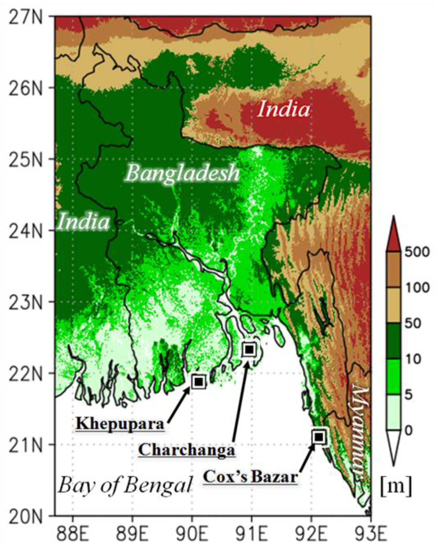
Global mean sea level (MSL) rise induced by climate change is an alarming issue with respect to the sustainability of the world’s coastal communities [1,2]. The global MSL is projected to increase by 0.52–0.98 m by the end of this century [3], which is anticipated to increase the risk of floods and deteriorate freshwater environments, particularly in low-lying regions. The Bangladesh coast is considered to be highly vulnerable to the adverse impacts of sea level rise [4,5,6]. Its geographical characteristics, with an active deltaic coast and low coastal elevation (1–5 m), make the area more vulnerable to sea level extremes [6,7] (Figure 1). Inadequate infrastructure and high population exposure also enhance the vulnerability of this area [5,8,9]. A one-meter increase in MSL by the late 21st century could affect approximately 1000 km2 of coastal areas in Bangladesh [10,11]. Therefore, it is essential to assess the magnitude of sea level extremes that are typically caused by meteorological and oceanic drivers.
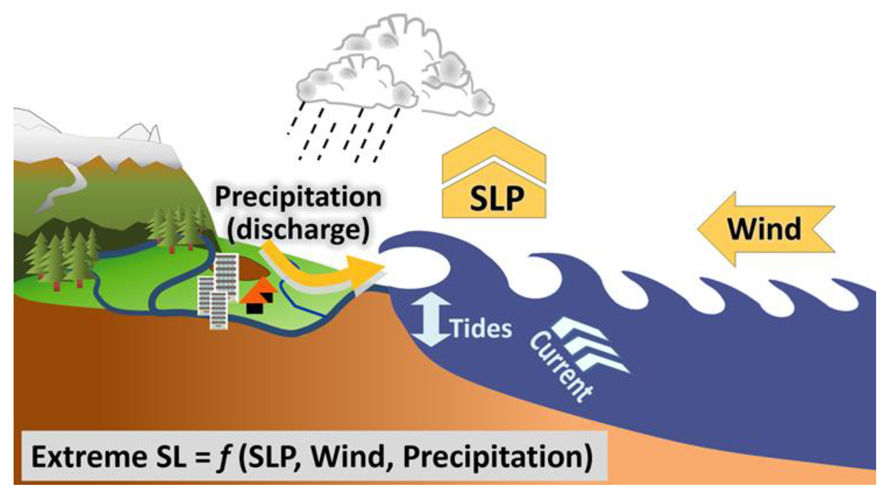
The review of the related literatures noted that the extreme sea level (hereafter referred to as ESL) mainly arises from the interactions of meteorological factors, such as low atmospheric pressure and high winds, and oceanic factors, such as tides, surges, and ocean currents [12,13,14,15,16,17,18]. Another factor related to the hydrological cycle is the discharge of precipitated water from continental upstream, which has been studied in many coastal areas across the world [19,20,21,22]. The contributing factors are illustrated in Figure 2. Among these factors, the effect of precipitation on ESL variability remains unexplored along the coast of Bangladesh, whereas other factors have been studied intensively [10,11,16,17,23,24,25,26,27]. The sensitivity experiment of the ocean model revealed that the river discharge affects the interannual variation of sea surface height near the river mouth [28]. The role of the ocean and atmospheric factors and precipitated water discharge to the long-term sea level variability along the coast of Bangladesh was addressed in earlier studies. However, the influence of terrestrial precipitation on ESL events at a daily time scale remains unknown. Therefore, the investigation of the precipitation effect on ESL events at a daily time scale represents the novelty of this study, and it is expected that the outcomes will contribute to improve the forecast of ESL events and disaster prevention.
Precipitation in and around Bangladesh has increased in recent decades [29,30,31] and is projected to have increased further by the late 21st century [32,33]. As a low altitude basin area of the three major river systems of the GBM (Ganges–Brahmaputra–Meghna) rivers, the coastal area of Bangladesh receives abundant precipitated water [34], which enhances the sea level near the coast and causes severe coastal flooding [6,8,9,25,30]. Hence, it is likely that the river discharge enhances the sea level in this region.
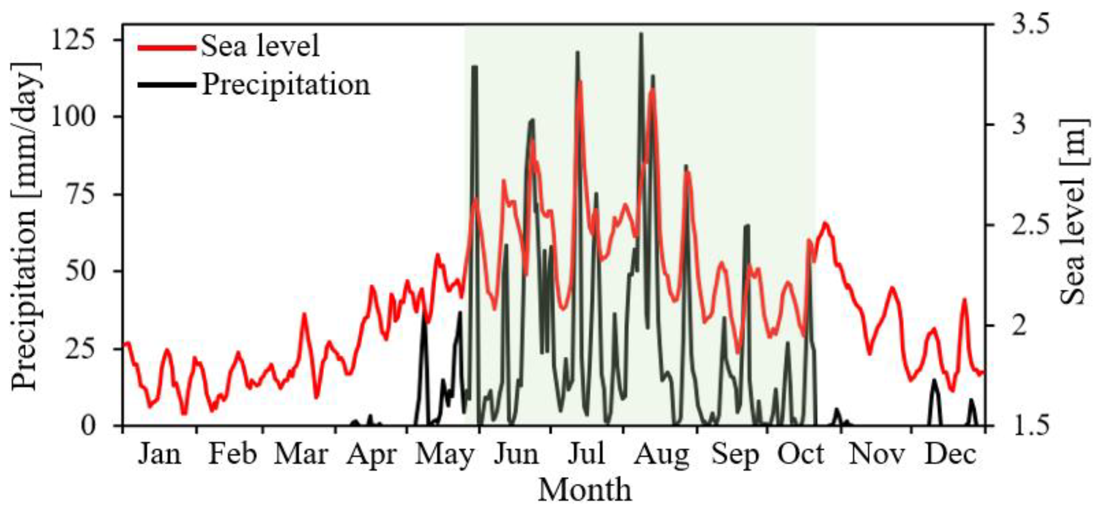
Figure 3 illustrates the seasonal variation of the daily sea level and precipitation in 1999, observed at Cox’s Bazar area (see Figure 1 for location). There are marked sea level peaks during the monsoon season, which appear to coincide with the precipitation peaks. The synchronized variation in daily sea level and precipitation shown in Figure 3 is a common characteristic observed in many other years. Figure 3 strongly suggests that precipitation enhances the sea level at a daily time scale, and its impact seems to be large for ESL events. Meanwhile, Figure 3 also suggests the role of other forcing factors. Strong precipitation events during the monsoon season are often caused by synoptic atmospheric disturbances [35], which have a potential to increase sea levels, even though precipitation-induced river discharge is absent, because the disturbances usually accompany changes in air pressure and wind speed. Considering this specific geographical background and high precipitation over this area, it is important to verify the contribution of precipitation variability during ESL events. Hence, the objective of this study was to investigate the effect of precipitation on ESL events at a daily time scale. The research was mainly conducted based on statistical analysis. It was hypothesized that the ESL prediction with the consideration of precipitation effect would outperform that without precipitation.
2. Materials and Methods
2.1. Data and Variables
The variability of ESL was investigated at three selected coastal sites. These sites are located in different geographical settings (Figure 1). Cox’s Bazar is located in the eastern coastal area and is characterized by a hilly landscape. Charchanga is located in the lower estuary of the GBM river system. Khepupara is located in the low-lying deltaic plain of the western coast. Daily station-observed sea level data, provided by the University of Hawaii Sea Level Center [UHSLC] [36], were used. The studied periods were 1983–2006 for Cox’s Bazar, 1980–2000 for Charchanga, and 1987–2000 for Khepupara, based on the availability of in-situ sea level data. The satellite-observed daily gridded (0.25° × 0.25°) anomalous sea level product of the Copernicus Climate Change Service (C3S) was adopted to investigate the spatial pattern of coastal sea levels during 1993–2006 [37].
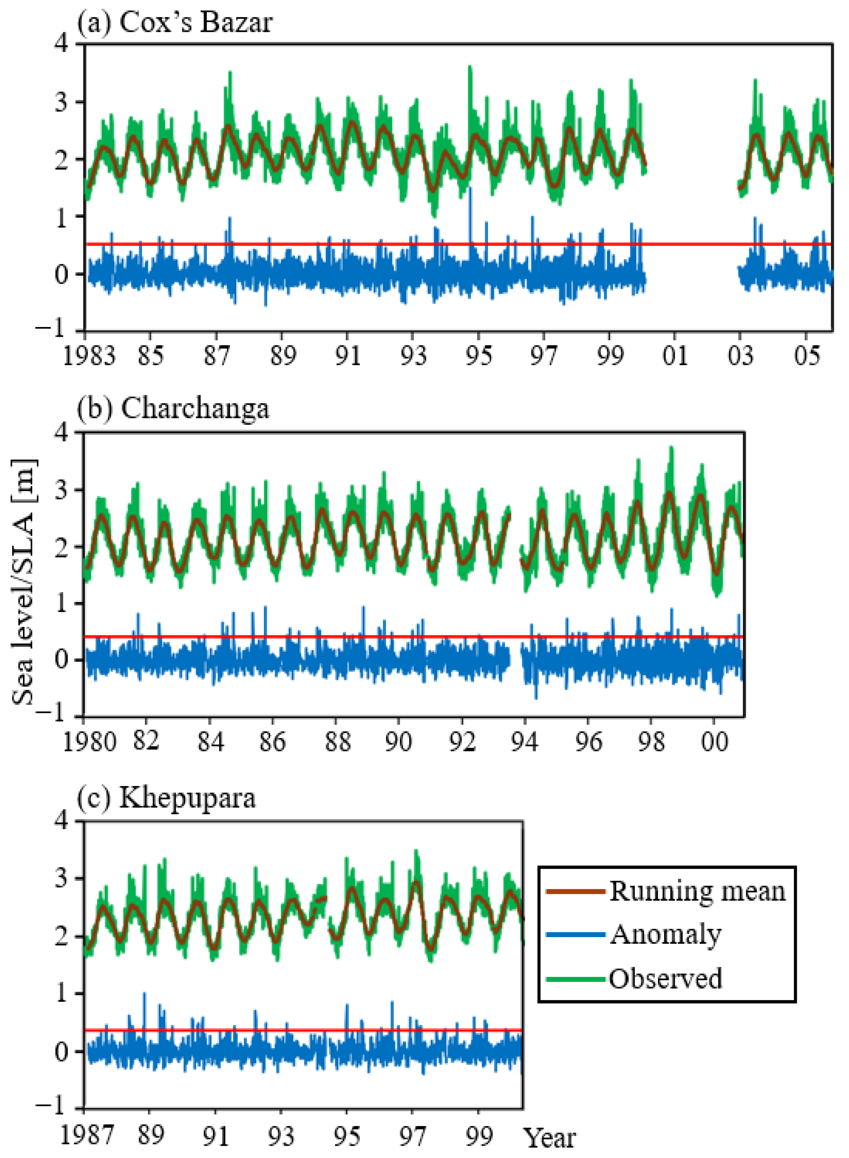
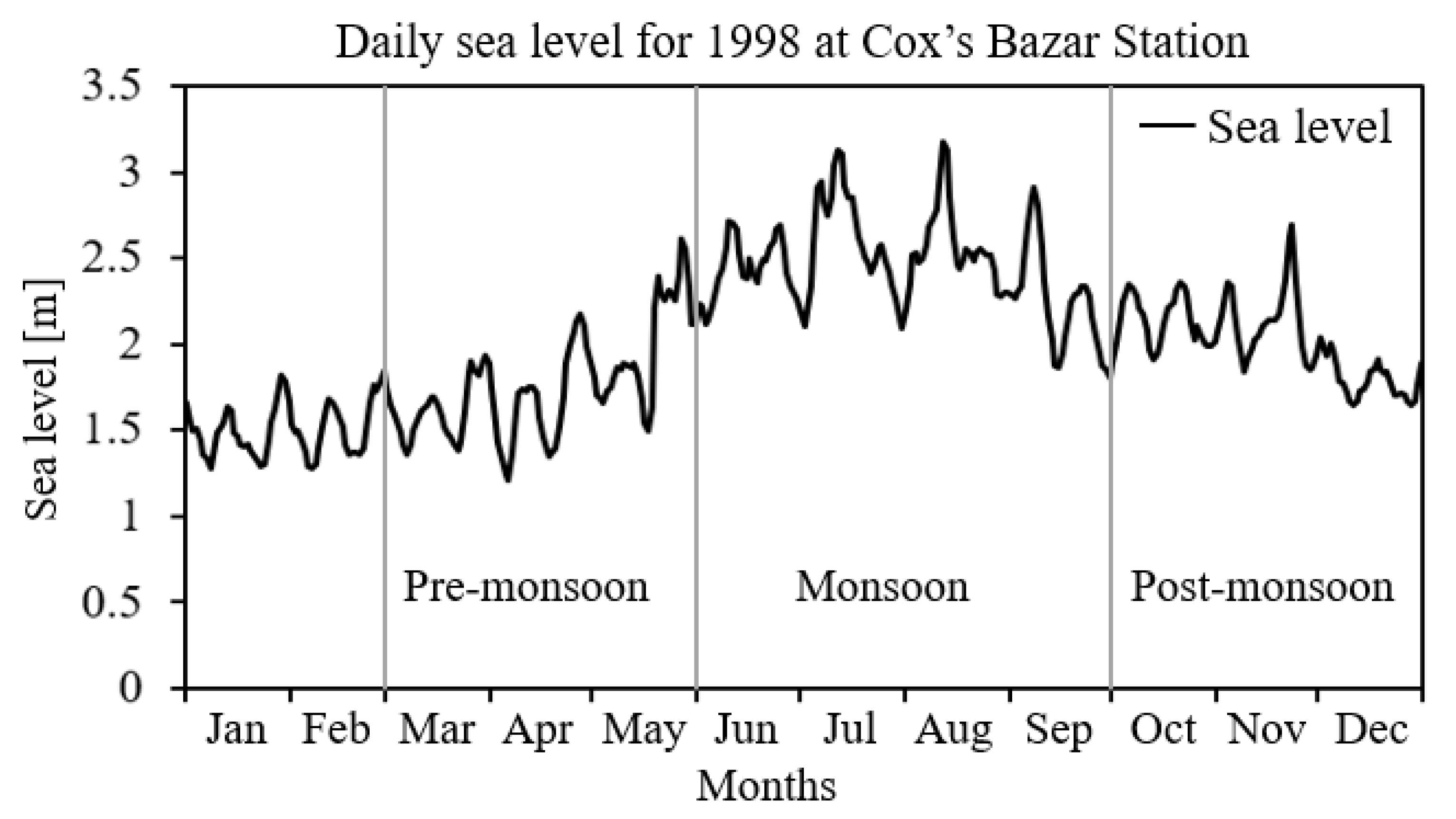
The sea level near the Bangladesh coast exhibits prominent seasonal variation [38] corresponding to the monsoon [39] and regular tidal cycles. An example of the seasonal variation of the daily sea level at Cox’s Bazar station for a one-year period of 1998 is shown in Figure A1. The figure shows a seasonal variation in sea level corresponding to pre-monsoon, monsoon, and post-monsoon seasons. To remove such low-frequency components, daily sea level anomalies (hereafter referred to as SLA) relative to the 91-day running mean were used. As demonstrated in Figure 4, the SLA represents the high-frequency daily sea level variations caused by meteorological factors and river discharge. Then, the ESL events were determined by applying the threshold value of the 99th percentiles in the daily SLA time series, following the method of previous studies [40,41]. The 99th percentile high SLA values were 0.562 m, 0.486 m, and 0.427 m (indicated by red lines in Figure 4), and the number of selected ESL events were 69, 62, and 37, respectively, for Cox’s Bazar, Charchanga, and Khepupara station.
Daily precipitation data were obtained from APHRODITE-V1003R1 [42], which covers land area at spatial resolution of 0.25° × 0.25°. The daily SLP and wind data were obtained from the Japanese 55-year Reanalysis [JRA55] [43], whose horizontal grid size is 1.25° × 1.25°. For precipitation, SLP, and winds, the area-averaged values over 20°–27° N and 87.7°–93° E were commonly used for all three sites. The area roughly corresponds to Bangladesh and is also a part of the hydrological catchment of GBM. At the determination of this area, we conducted a pre-analysis, aiming to identify the source area from where the precipitated water could influence the sea level. We found that the daily sea level for the periods of extreme events was highly correlated with the daily precipitation over the lower river basin of the GBM covering the Bangladesh area (not shown). This convinced us that the domain setting for the area-average was reasonable. This result may also reflect the effects of humans’ control of river water in the upper river basin [44,45,46], which results in a low correlation between sea level and precipitation in the upper-river basin.
2.2. Empirical Methods
A multivariate linear regression (MLR) analysis was used to investigate the effect of precipitation on the daily variability of sea level during the extreme events. The MLR has been widely used to discuss the mechanisms of sea level variations at various timescales [18,47,48]. Using MLR statistics, the targeted variable (observed daily SLA) could be described by the linear combination of explanatory variables. Previous studies analyzed the linear relationship between sea level and explanatory variables of sea level pressure (SLP), precipitation, air temperature, winds, and climate variability indices [18,48,49,50]. Here, we selected four explanatory variables: precipitation, SLP, zonal wind (U), and meridional wind (V), and we evaluated their influences on sea level variations. To represent the characteristics of the used dataset for the selected ESL events, a summary of descriptive statistics of the variables at each of the three stations has been added in Section S1. It might be best if we can incorporate river discharge as an additional explanatory variable for more skillful MLR. However, the river discharge data were unavailable in the upstream regions of the targeted sea level stations. The prediction equation for the observed SLA is described as
SL’(t) = a1 × SLP(t) + b1 × U(t) + c1 × V(t) + d1 × Pre(t) + e1
Herein, t represents the duration of the event, which ranged from −6 to 0, corresponding to six days before the targeted ESL (t = −6) to the day of the ESL event (t = 0). As indicated in Equation (1), our focus was the seven-day variation of SLA and its controlling factors. This time range was determined by considering the fact that the durations of the ESL events are generally around a week, probably reflecting the life span of storm-induced surges and cyclones [18,48]. SL’ represents the predicted SLA. Pre represents the accumulated precipitation over the preceding five days for each t, to account for the delayed effect of runoff after precipitation. According to our pre-analysis, it was found that the setting of five-day accumulated precipitation outperformed in comparison with other possible settings regarding the length of the preceding days (Figure A2). This result may imply that the typical time scale of river discharge over this rain-prone area is approximately five days, although this hypothesis needs to be investigated using reliable river discharge data. The explanatory variables were standardized, and the MLR analysis was performed for each ESL event. The regression coefficients are represented as a, b, c, and d, while e represents the intercept value. The coefficients were determined for each site and for each selected event.
To elucidate the impact of precipitation on the SLA, another MLR analysis was conducted. Without the precipitation effect (Pre), the MLR equation is rewritten as
SL’(t) = a2 × SLP(t) + b2 × U(t) + c2 × V(t) + e2
The predicted sea level anomalies obtained from MLR Equations (1) and (2) were evaluated using the same seven-day time series of the observed daily SLA as reference data. The goodness of fit of each prediction was evaluated by R2. The R2 values were expected to be different between two predictions, and an R2 close to one denotes that the MLR is very skillful. If the prediction using Equation (1) outperforms the prediction using Equation (2), it means that adding precipitation data could improve the prediction of SLA during the ESL event. It was anticipated that the contribution of precipitation to the prediction of ESL may be influenced by the multicollinearity of the variables. To argue this point, we performed a correlation analysis among the variables for each ESL event of the three study stations (Section S2). It showed that the correlation among the explanatory variables was not significant in the majority of the events, which denoted the independency of the explanatory variables in the MLR (Table S4). In this study, the difference in R2 between the two predictions was regarded as the significance of the effect of precipitation. If R2 for the prediction with precipitation (i.e., Equation (1); hereafter referred to as WP) is greater than that without precipitation (i.e., Equation (2); hereafter referred to as WOP), we can consider that precipitation is crucial for the targeted extreme event. Thus, a larger difference in R2 between predictions WP and WOP denotes a stronger influence of precipitation on sea level variations. The R2 value was evaluated for all selected events to determine the spatial and temporal characteristics of the effect of precipitation on the sea level. One may anticipate that the difference in R2 simply reflects the difference in the number of explanatory variables between Equations (1) and (2), rather than the precipitation effect. We have argued this point in Section 4.
In addition to the MLR analysis, the influence of remote and local sea surface temperature (SST) was analyzed to investigate the relationship between SST and interannual variabilities of high sea level and precipitation in the studied region. To explore the role of large-scale atmosphere–ocean coupled modes, the Oceanic Niño Index [ONI] [51] and the Dipole Mode Index [DMI] [52] were obtained from the National Weather Service and Physical Sciences Laboratory of NOAA, respectively. Aside from these remote SST effects, local SST in the Bay of Bengal was also analyzed for the above-mentioned purpose. For this, we use Optimum Interpolation Sea Surface Temperature [OISST] [53] data from NOAA.
3. Results
3.1. Influence of Precipitation in Selected Cases
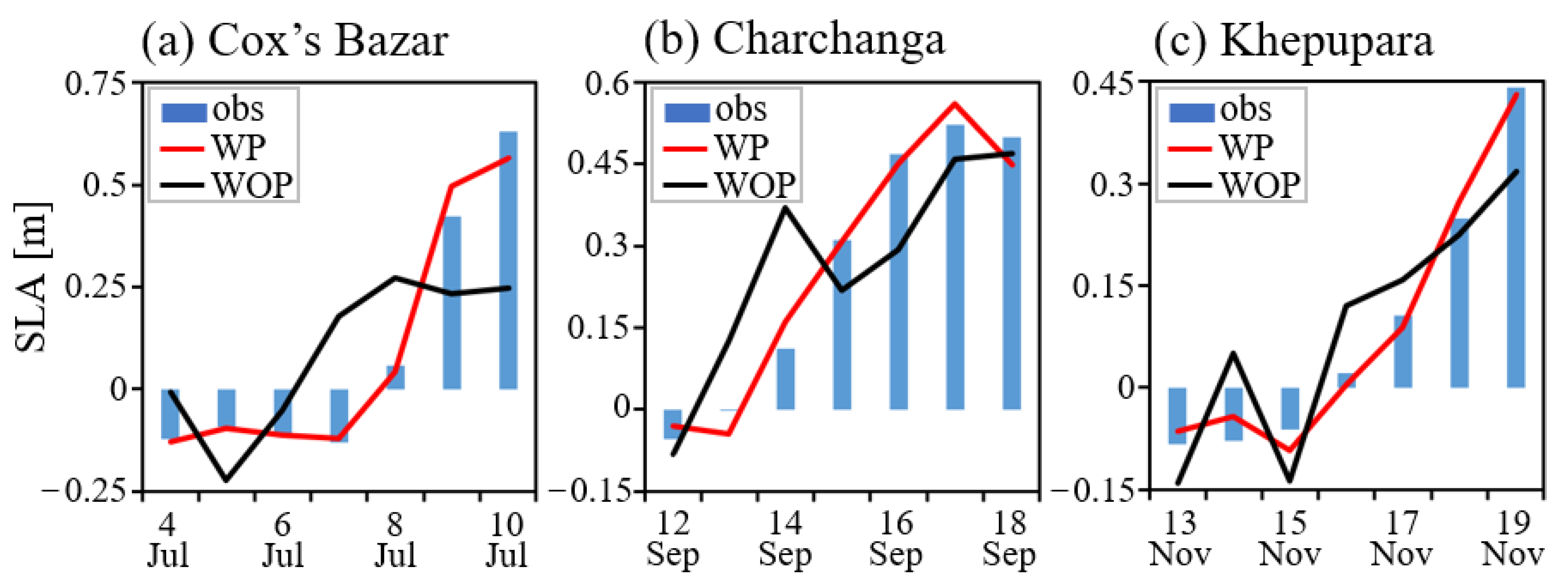
In this section, the effect of precipitation on SLA was evaluated using MLR statistics. Figure 5 compares the variations of predicted and observed sea levels for a typical event at each station. Here, we only presented successful cases, in which the sea level prediction was nicely improved by adding the precipitation effect. We will later examine all extreme cases to see under what condition the effect of precipitation plays a crucial role. At Cox’s Bazar, the observed daily sea level on 10 July 2006 was well captured by the prediction with precipitation (i.e., Equation (1)), which achieved R2 = 0.982 (Figure 5a), and the root mean squared error (RMSE) was 0.03. This result suggests that the evolution of ESL was mainly controlled by meteorological factors. However, when the effect of precipitation was excluded, the R2 decreased to 0.371 (Figure 5a), and the RMSE became 0.23. At Charchanga on 18 September 1997, the prediction with precipitation was more skillful (R2 = 0.974, RMSE = 0.04) than the prediction without precipitation (R2 = 0.645, RMSE = 0.13) (Figure 5b). At Khepupara on 19 November 1988, the prediction with precipitation also performed better, although the differences in R2 between the prediction with (R2 = 0.983, RMSE = 0.02) and without precipitation (R2 = 0.772, RMSE = 0.09) were small (Figure 5c) compared with those of Cox’s Bazar and Charchnaga stations. The difference in R2 between the two predictions implies that the impact of precipitation on ESL differed for each station. We decomposed the MLR Equation (1) to understand the causality of the precipitation effect for the predictions of ESL (Section S3). Figure S1 confirms that the influence of precipitation on sea level rise during the ESL event was larger than the influence of other atmospheric forces.
3.2. Evaluation of the Predictability for All Events
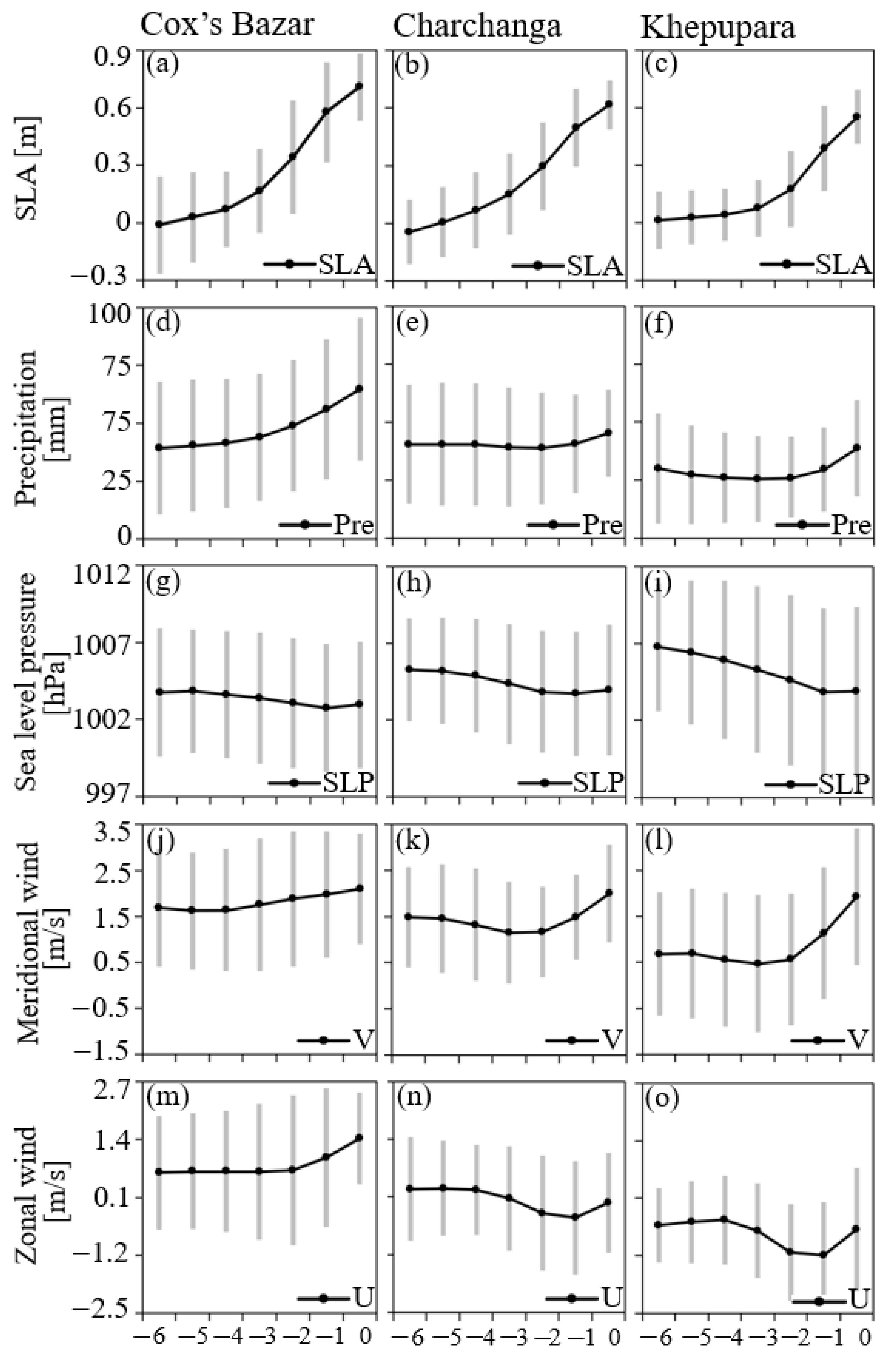
In Section 3.1, we confirmed that the consideration of precipitation could enhance predictability of the sea level for selected events. Here, a composite analysis for all ESL events was performed to understand the spatiotemporal variations of sea level and forcing parameters. Figure 6 displays the time series of SLA and meteorological variables, averaged for all selected ESL events. For all three of the stations, the mean SLA was highest on the day of the extreme (t = 0), with a gradual increase from the prior days (Figure 6a–c). The precipitation at Cox’s Bazar showed a similar evolution with SLA, in which the amount of precipitation increased gradually towards the day of ESL (Figure 6d). In comparison with Cox’s Bazar, the evolutions of precipitation for Charchanga (Figure 6e) and Khepupara (Figure 6f) did not show such a monotonic increase. The time series of SLP at all three stations showed a gradual decline from the prior days to the day of the extreme (Figure 6g–i), suggesting that a low-pressure system was approaching the targeted area. The SLP decrease was relatively steady at Khepupara (Figure 6i). The southerly wind velocities at the three stations increased and reached the maximum on the day of ESL (Figure 6j–l). In Charchanga and Khepupara, the southerly wind was intensified from t = −2, denoting a strong effect of a wind-induced surge for these locations. The westerly wind increased during the ESL events at Cox’s Bazar, while the zonal wind speed was near zero at Charchanga, and an easterly wind was dominated at Khepupara (Figure 6m–o).
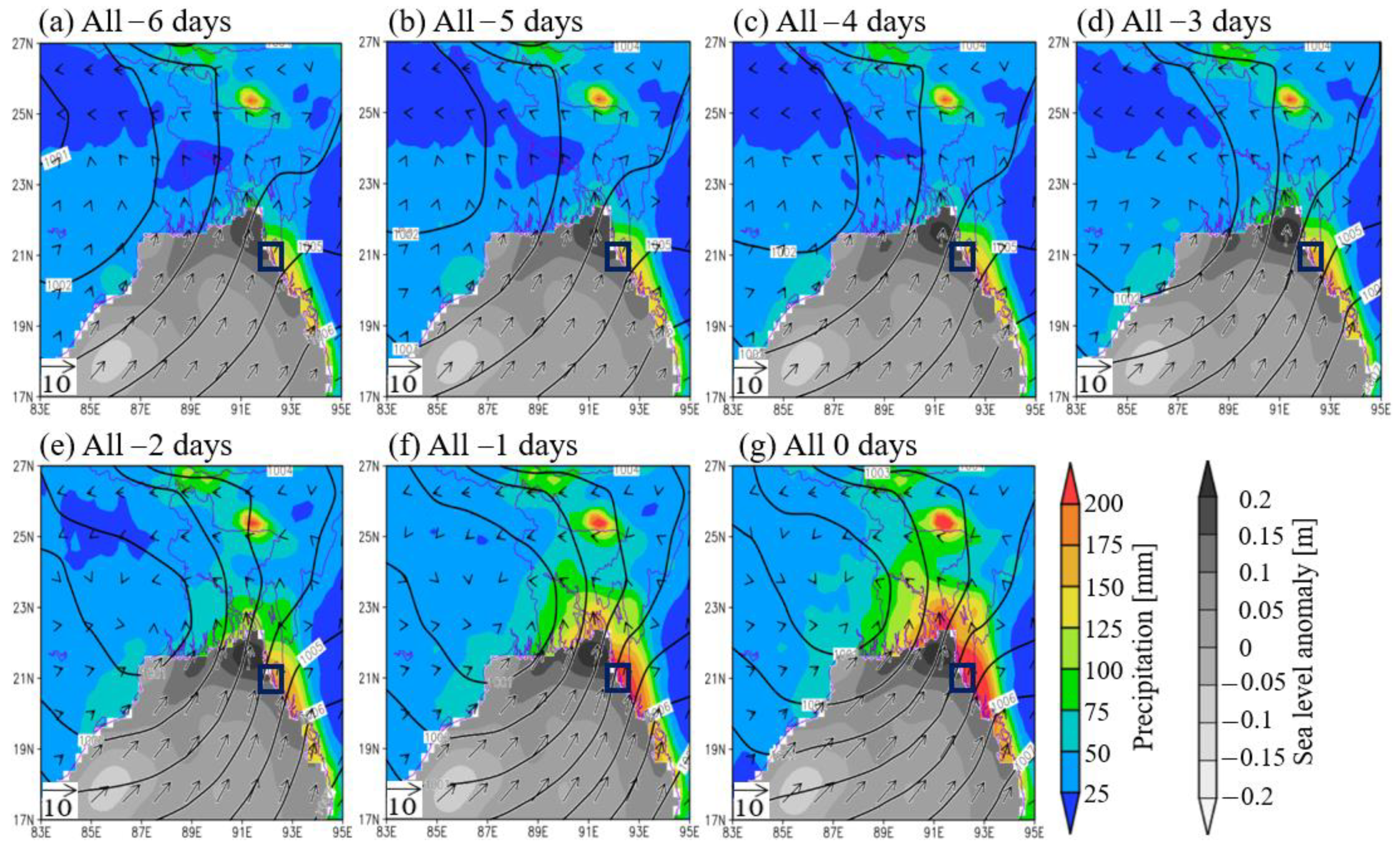
Similarly, a composite spatial distribution of meteorological variables has been presented for ESL events at Cox’s Bazar. The composite analysis was performed for the period of 1993–2006, considering the availability of SLA data. Please note that the definition of sea level anomaly for the daily gridded data, which represents the deviation of the daily sea level from 20-year mean, was different from the one used for the station data (Section 2). Figure 7 demonstrates that the sea level anomaly along the coast was high throughout the targeted seven-day duration and increased until the day of ESL, which was consistent with the time evolution in the station data (Figure 6a). Accumulated precipitation over the coastal area remained high from t = −6 through to t = 0, presumably reflecting the strong enhancement of orographic rain along the Arakan Mountains [54]. The rainfall began to increase from t = −1 and reached a maximum on the ESL day (Figure 7a–g). The high orographic rain appeared to be intensified in accordance with strong southerly-southwesterly winds toward the coast, which are part of synoptic-scale flow surrounding the low-pressure center, located over western India (Figure 7g). The composite analysis suggests that high precipitation concentrated on the narrow hilly slope increased SLA along the coast of Cox’s Bazar, together with the effects of low SLP and associated surface winds. The earlier studies also mentioned that the storm-induced surges, associated with low pressure and high winds, accelerate the sea level rise along the coast of Bangladesh [10,15,16,17,27].
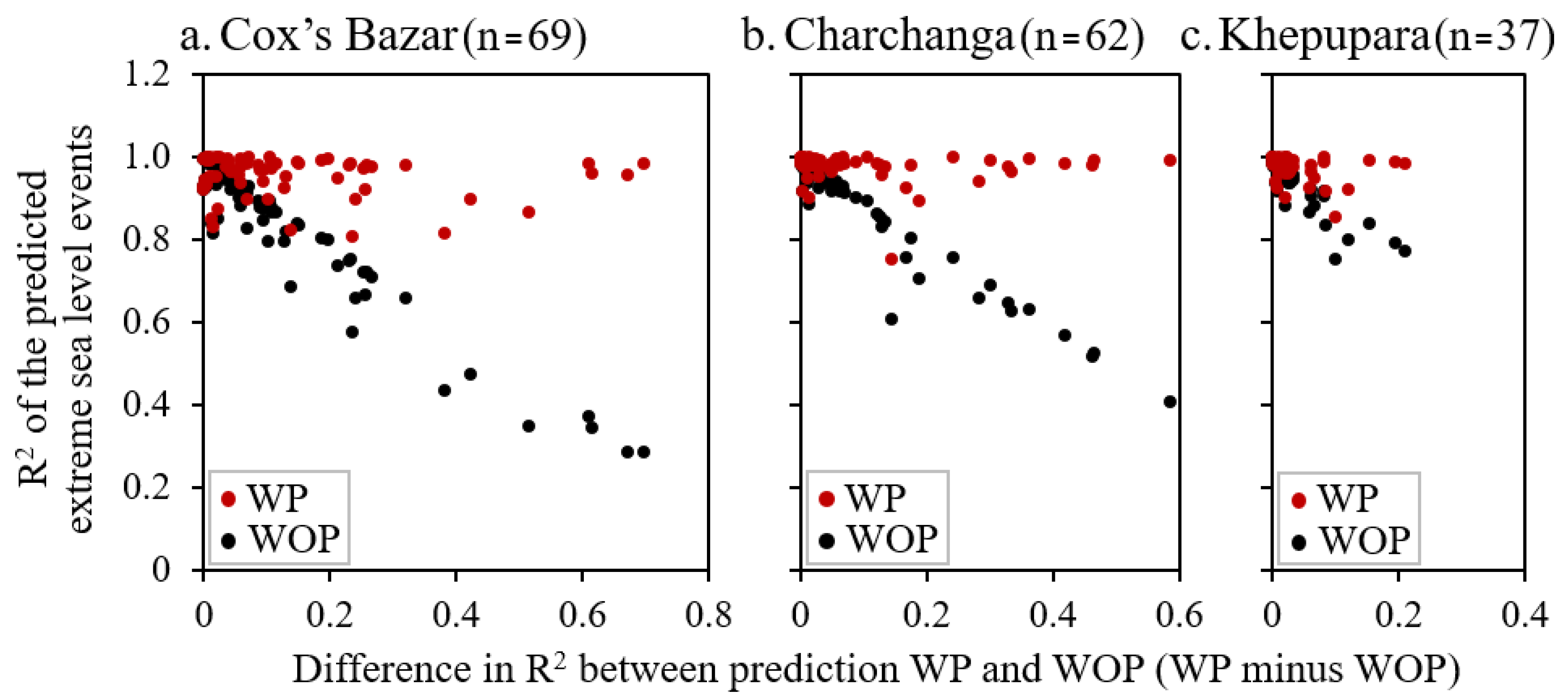
Figure 8 examines the R2 of the SLA predictions for all extreme events. The higher R2 was commonly seen for the prediction with precipitation. This was a common character for the root mean square error (RMSE, Table 1). The distribution of RMSE values for the predictions with precipitation shifted lower in comparison to that for the prediction without precipitation; the lower shift of the mean RMSE value was statistically significant (p < 0.05 for the three stations). These results show the importance of precipitation variability in predicting sea level variation along the coast of Bangladesh. The improvement in R2 for WP predictions was greater at Cox’s Bazar than at Charchanga and Khepupara. Figure 8 shows that the increase of R2 was large for the event whose R2 value was low for the prediction WOP. For such cases, the daily variation of sea level is likely to be influenced by the precipitation that accompanies river discharge, and therefore, the consideration of the precipitation effect would improve the predictability of ESL. Studies have shown that the high river discharge modulates the long-term sea level variability along the coast of Bangladesh [24,25,28,33]. Our emphasis was, however, on the daily sea level variation. We recognize that, in a few cases, the R2 was not so high, even with the consideration of precipitation (Figure 8). For such cases, nonlinear effects may play an important role, and our MLR did not work as expected.
3.3. Seasonal Variations of the Impact of Precipitation
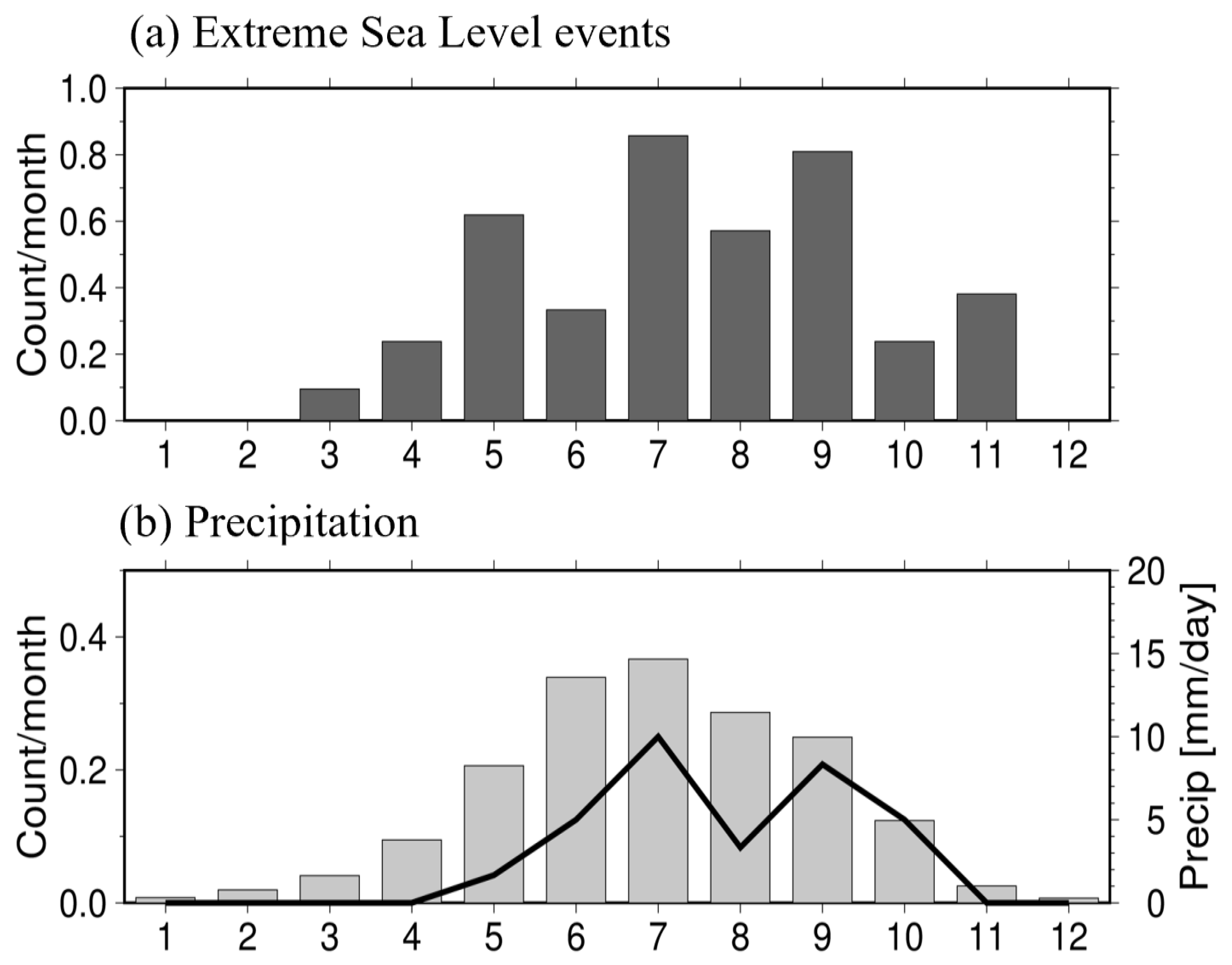
In this section, the impact of precipitation on ESLs has been evaluated, with a focus on the seasonal variability of precipitation. Figure 9 shows the seasonal variation of precipitation over Bangladesh (20°–27° N and 87.7°–93° E). Monthly precipitation in Bangladesh has high seasonal variability, associated with summer monsoon, which typically ranges from June through to September (Figure 9b). According to the submonthly-scale intraseasonal variability dominant in this region [55], there is a prominent increase of heavy precipitation events (>50 mm/day) from pre-monsoon (May) to post-monsoon (October) seasons. The frequency of ESL events showed a similar seasonal variation with the heavy precipitation event, indicating that ESL events are triggered by high precipitation events (Figure 9a). The seasonal variation of high precipitation was also noticed in earlier studies [29,38,56,57,58].
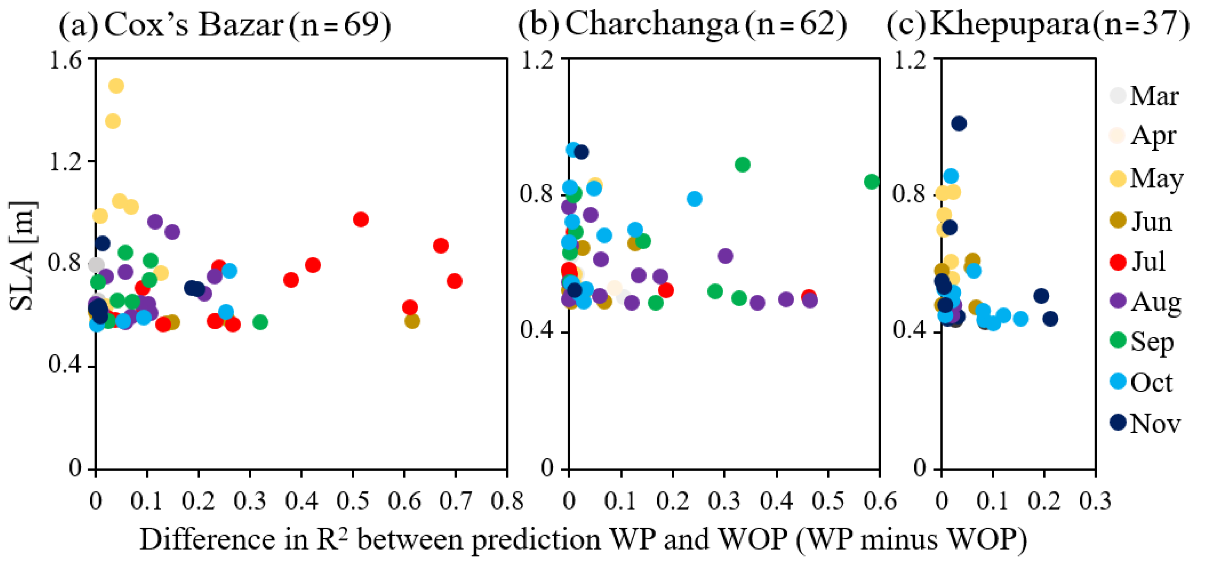
Figure 10 shows the relationship between SLA and the R2 difference between two predictions. Here, we used the difference as a measure to quantify the influence of the precipitation effect (c.f., Section 2). In Cox’s Bazar, ESL events with a high influence of precipitation tended to occur in June and July (Figure 10a), corresponding to the peak precipitation during the summer monsoon (Figure 9b). Figure 9a,b also confirmed that the simultaneous increases of ESL events and heavy precipitation in 1999, as shown in Figure 3, are common characters for many years. Interestingly, the highest SLAs were observed in May (Figure 10a), and the difference in R2 for these events was generally small. We confirmed that these events mostly occurred in early May in 1995 and 1997, and there were tropical cyclones or tropical depressions over the study area [59,60]. Hence, it is very likely that these ESL events were strongly influenced by SLP and winds, rather than the precipitation effect. For such cases, since R2 was originally very high, predictions WP and WOP did not differ largely. In June and July, the effect of precipitation at Cox’s Bazar was thought to be enhanced because the precipitation amount was high in these months (Figure 9b). In Charchanga, the ESL events with a large R2 difference occurred during the post-monsoon period from August through to September (Figure 10b). The frequency of heavy precipitation events remained high in these months, leading to the possibility of a large contribution of precipitation. At Khepupara, the differences in R2 were found during October and November, corresponding to the post-monsoon season, although the magnitude of the R2 difference was smaller than other stations (Figure 10c). The impact of precipitation on the skill of MLR predictions varied among stations and seasons. It has been suggested that the impact was high in Cox’s Bazar and Charchanga for July and September–October, respectively. These months agree well with the month of highest precipitation for the study area (Figure 9b), as mentioned in previous studies [30,57,58].
3.4. Influence of Remote and Local SST
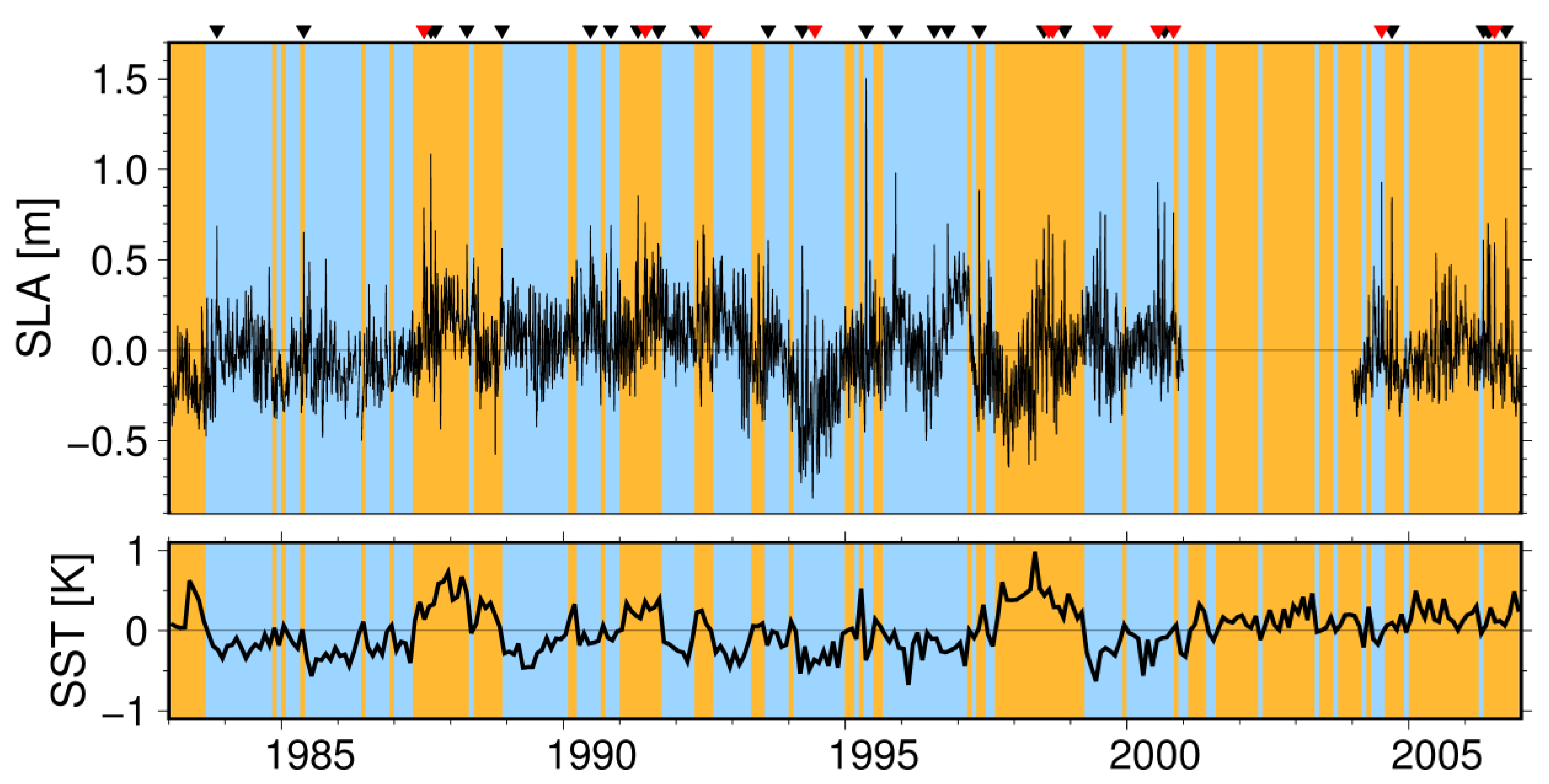
In Section 3.3, we confirmed that the predictability of ESL varies with the seasonal march of monsoonal precipitation. It is known that the monsoonal precipitation shows interannual variation in relation to large-scale ocean and atmosphere dynamics [56,61,62]. This section describes the influence of remote and local SSTs on ESL events and precipitation. Figure 11 depicts the interannual time series of the daily SLA at Cox’s Bazar. Although it is not clear in Figure 11, we confirmed that the occurrence of positive SLA was more frequent during the years with a high SST anomaly (>0.5 K, 5.2%) than with a low SST anomaly (<−0.5 K, 2.0%) in the Bay of Bengal. However, the SST’s impact on ESL remains unclear because the ESL events seemed to occur irrespectively of the SST anomaly (Figure 11). It is expected that the SST serves as an indirect forcing agent for ESL, through enhancing the cyclone activity and high precipitation when SST in the Bay of Bengal is high [62,63,64]. The difference in R2 also seemed to be independent of the local SST (Figure 11). To clarify the reason for this weak connection between the SST and the impact of precipitation to ESL, we next examined the relationship between SST and precipitation.
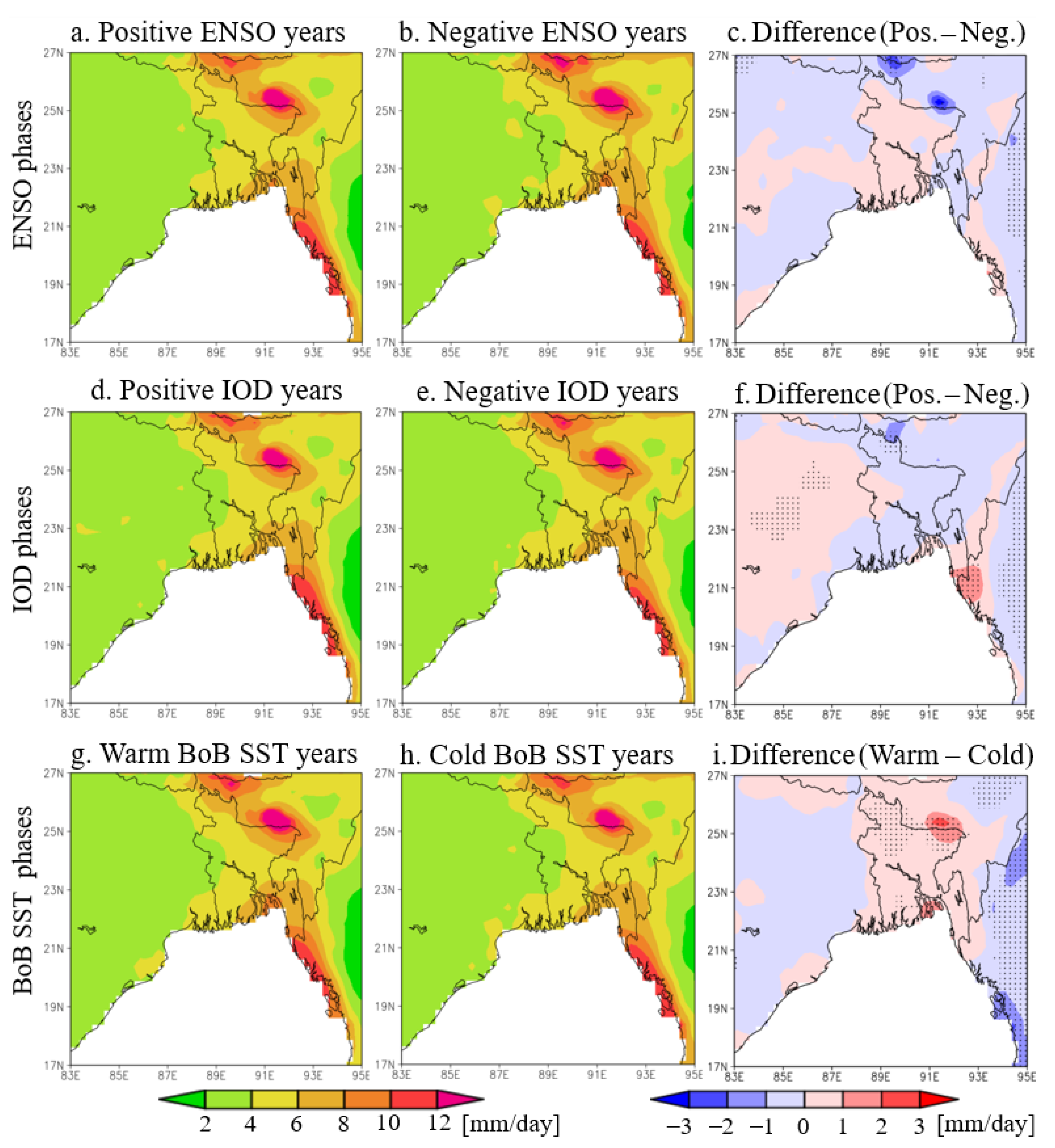
Considering the importance of precipitation for a high SLA, spatial distributions of terrestrial precipitation were investigated for remote SST (i.e., ENSO and IOD) and local SST conditions. A list of the status for ENSO/IOD and local SST during 1983–2006 is given in Table 2. There was no significant difference in precipitation over the area of Bangladesh between the positive and negative phases of ENSO and IOD (Figure 12a–c), suggesting that the effect of remote SST was not a dominant factor altering the terrestrial precipitation variability over Bangladesh. For the positive IOD phase, a positive precipitation anomaly was found only in a narrow area near Cox’s Bazar (Figure 12d–f). Such a weak response of precipitation to remote SST has been noted by previous studies [56,57,65]. Our composite analysis indicated that the passage of cyclones with a low SLP and high meridional wind enhances the SLA (Figure 7g). Studies have found that the passage of tropical cyclone is frequent during negative ENSO and negative IOD [66,67]. Hence, the ENSO and IOD modulate the cyclone activity, and the direct influence of cyclones on ESL might explain the indirect impacts of SST. It was found that when the local SST in the Bay of Bengal is warmer, the northern Bangladesh area receives more precipitation (Figure 12g–i). The precipitation enhancement over these hilly areas is regulated by the mesoscale atmospheric circulation, governed by submonthly-scale intraseasonal variability and the diurnal cycle [68]. The enhanced precipitation and the resultant increase in river discharge could help increase the sea level along the coast [24,28]. Therefore, the frequency of ESL events tends to be high during warm SST years. It is expected that in future, the consideration of the discussed role of local and remote SST will be important for studying the ESL variability in this region.
4. Discussion
In Section 3.2, we confirmed that the R2 for prediction WP was higher than that for WOP. The increased R2 might have resulted from the utilization of an increased number of explanatory variables in WP predictions in comparison with WOP predictions rather than the physical contribution of precipitation to sea level. To evaluate the robustness of the higher R2 values in WP predictions, an additional analysis using adjusted R2 statistics [69] was performed. It was hypothesized that if the adjusted R2 is close to the original R2, it means that R2 is not influenced by the number of explanatory variables. The adjusted R2 was calculated by
Herein, p is the number of explanatory variables, and n is the sample size. We assumed p = 4 (i.e., SLP, zonal and meridional winds, and precipitation) for the sea level prediction WP, whereas p = 3 was assumed for the prediction WOP. The sample size was set as n = 7, considering the seven-day variations of meteorological variables (see Section 2). The adjusted R2 for predictions with precipitation data were higher than those without precipitation data for 50 (72% relative to the total ESL events), 34 (55%), and 20 (54%) events in Cox’s Bazar, Charchanga, and Khepupara, respectively. Hence, we conclude that precipitation is likely to be an essential factor for ESL at Cox’s Bazar for a majority of the ESL events. In contrast, for other stations, the benefit of precipitation data appeared to be limited in up to approximately half of the ESL events. Negative values in the adjusted R2 were found for WOP prediction (7 out of 69 and 1 out of 62 events, respectively, for Cox’s Bazar and Charchanga). These negative values mean that the sea level was not well predicted without accounting for precipitation. The number of events with a high adjusted R2 (≥0.9) was significantly greater in WP predictions than WOP predictions (Table 3). This also supports our earlier speculation that the effect of precipitation improves the predictability of ESL events. In addition, we believe the adoption of a physical model is desirable to understand the causality of precipitation to increase ESL. However, the consideration of such a physical model is beyond the scope of this study.
5. Conclusions
The present study investigated the influence of precipitation on ESL along the coast of Bangladesh using MLR statistics. It was revealed that the estimation of ESLs considering precipitation effects outperformed the estimation of ESLs without precipitation. This study revealed that the influence of precipitation on extreme SLA is higher at Cox’s Bazar than at Charchanga and Khepupara. The effect of high precipitation at Cox’s Bazar reflects its hilly landscape that accelerates runoff and enhances coastal water levels with inundation [4,6,24,58]. It was found that the ESLs were influenced by the high precipitation during the monsoon season. The extreme sea levels intensify coastal inundation and cause coastal floods with high precipitation during monsoons [8,32,57,59,65]. Therefore, the attempt of this study relating to predictions of ESL has implications for the reduction of coastal hazards. Our results demonstrated that the effect of precipitation on ESL is robust, and the effect of precipitation on the variability of sea levels has spatial variation, with strong effects in the central and eastern parts of the coast. The revealed spatial variability in sea level may be helpful for the planning of coastal management.
This study investigated the possible effect of terrestrial precipitation of daily ESL for many events. It is widely known that this region is one of the wettest regions in the world [29,56,58], having a peak precipitation associated with the summer monsoon. Fujinami et al. [70] pointed out that sub-monthly intraseasonal precipitation variability shows a significant contribution to the variability of annual precipitation. It is hoped that future studies will analyze the possible influence of intraseasonal precipitation variability to improve the predictability of sea level variations.
Supplementary Materials
The following are available online at https://www.mdpi.com/article/10.3390/w13202915/s1: Section S1: Represents the descriptive statistics of the used dataset for the selected ESL events at three study stations. Section S2: Represents the contribution of each MLR term to daily seal level evolution. Section S3: Exhibits the correlation analysis among the explanatory variables for all ESL events at three study stations.
Author Contributions
Conceptualization, methodology, M.A.I. and T.S.; software, M.A.I.; validation, M.A.I.; investigation, M.A.I. and T.S.; resources, formal analysis, data curation, writing—original draft preparation, M.A.I.; writing—review and editing, M.A.I. and T.S.; visualization, M.A.I. and T.S.; supervision, project administration, funding acquisition, T.S. All authors have read and agreed to the published version of the manuscript.
Funding
This research was funded by Japan Society for the Promotion of Science (KAKENHI) Grant Number 18KK0098.
Institutional Review Board Statement
Not applicable.
Informed Consent Statement
Not applicable.
Data Availability Statement
The datasets used in this study are all publicly available via the internet.
Acknowledgments
M.A.I. acknowledges the scholarship support provided by the Ministry of Education, Culture, Sports, Science, and Technology, Japan.
Conflicts of Interest
The authors declare no conflict of interest.
Appendix A
Figure A1.
Time series for the seasonal variation of sea levels in 1998 at Cox’s Bazar Station. The sea level is varied by the seasonal effects of the pre-monsoon (March–May), monsoon (June–September), and post-monsoon (October–December).
Figure A1.
Time series for the seasonal variation of sea levels in 1998 at Cox’s Bazar Station. The sea level is varied by the seasonal effects of the pre-monsoon (March–May), monsoon (June–September), and post-monsoon (October–December).

Figure A2.
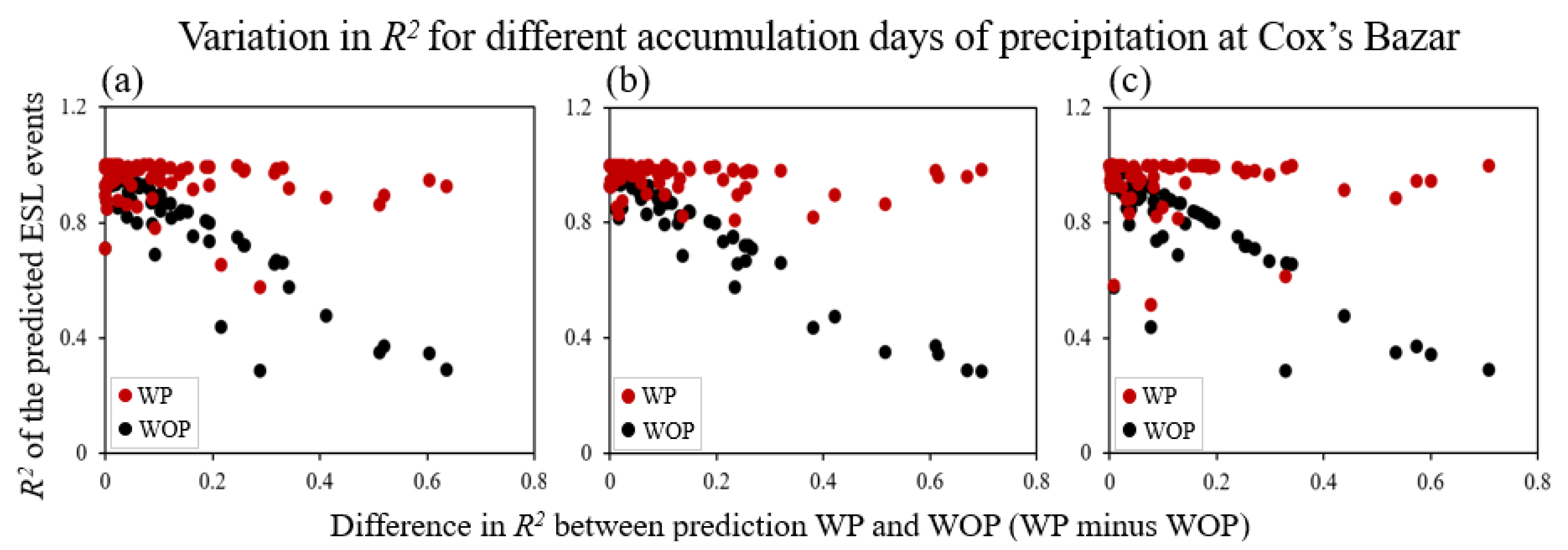
The relationship between the R2 values of sea level predictions at Cox’s Bazar, based on MLR for WP and WOP, using different accumulation days for precipitation. In (a), 3 days of accumulated precipitation was used. (b,c) same as (a) but for 5 days and 7 days, respectively. Each dot corresponds to an ESL event. Red and black dots represent the R2 for predictions WP and WOP, respectively. The y-axis represents the R2 for predictions WP. The x-axis represents the differences in R2 between WP and WOP predictions.
Figure A2.
The relationship between the R2 values of sea level predictions at Cox’s Bazar, based on MLR for WP and WOP, using different accumulation days for precipitation. In (a), 3 days of accumulated precipitation was used. (b,c) same as (a) but for 5 days and 7 days, respectively. Each dot corresponds to an ESL event. Red and black dots represent the R2 for predictions WP and WOP, respectively. The y-axis represents the R2 for predictions WP. The x-axis represents the differences in R2 between WP and WOP predictions.

References
- Wahl, T.; Haigh, I.D.; Nicholls, R.J.; Arns, A.; Dangendorf, S.; Hinkel, J.; Slangen, A.B.A. Understanding Extreme Sea Levels for Broad-Scale Coastal Impact and Adaptation Analysis. Nat. Commun. 2017, 8, 16075. [Google Scholar] [CrossRef]
- Wu, S.Y.; Yarnal, B.; Fisher, A. Vulnerability of Coastal Communities to Sea-Level Rise: A Case Study of Cape May County, New Jersey, USA. Clim. Res. 2002, 22, 255–270. [Google Scholar] [CrossRef]
- IPCC. Climate Change 2013: The Physical Science Basis: Contribution of Working Group I to the Fifth Assessment Report of the Intergovernmental Panel on Climate Change; Stocker, T.F., Qin, D., Plattner, G.-K., Tignor, M., Allen, S.K., Boschung, J., Nauels, A., Xia, Y., Bex, V., Midgley, P.M., Eds.; Cambridge University Press: Cambridge, UK; New York, NY, USA, 2013; p. 1535. [Google Scholar]
- Karim, M.F.; Mimura, N. Impacts of Climate Change and Sea-Level Rise on Cyclonic Storm Surge Floods in Bangladesh. Glob. Environ. Chang. 2008, 18, 490–500. [Google Scholar] [CrossRef]
- Sarwar, M.G.M. Sea-Level Rise along the Coast of Bangladesh. In Disaster Risk Reduction Approaches in Bangladesh; Shaw, R., Mallick, F., Islam, A., Eds.; Springer: New York, NY, USA, 2013; pp. 217–231. [Google Scholar]
- Brammer, H. Bangladesh’s Dynamic Coastal Regions and Sea-Level Rise. Clim. Risk Manag. 2014, 1, 51–62. [Google Scholar] [CrossRef]
- Rasid, H.; Pramanik, M.A.H. Visual Interpretation of Satellite Imagery for Monitoring Floods in BANGLADESH. Environ. Manag. 1990, 14, 815–821. [Google Scholar] [CrossRef]
- Mirza, M.M.Q. Three Recent Extreme Floods in Bangladesh: A Hydro-Meteorological Analysis. Nat. Hazards 2003, 28, 35–64. [Google Scholar] [CrossRef]
- Dastagir, M.R. Modeling Recent Climate Change Induced Extreme Events in Bangladesh: A Review. Weather Clim. Extrem. 2015, 7, 49–60. [Google Scholar] [CrossRef]
- Unnikrishnan, A.S.; Kumar, M.R.R.; Sindhu, B. Tropical Cyclones in the Bay of Bengal and Extreme Sea-Level Projections along the East Coast of India in a Future Climate Scenario. Curr. Sci. 2011, 101, 327–331. [Google Scholar]
- Antony, C.; Unnikrishnan, A.S.; Woodworth, P.L. Evolution of Extreme High Waters along the East Coast of India and at the Head of the Bay of Bengal. Glob. Planet. Chang. 2016, 140, 59–67. [Google Scholar] [CrossRef]
- Moron, V.; Ullmann, A. Relationship between Sea-Level Pressure and Sea-Level Height in the Camargue (French Mediterranean coast). Int. J. Clim. 2005, 25, 1531–1540. [Google Scholar] [CrossRef]
- Han, W. Origins and Dynamics of the 90-Day and 30-60-Day Variations in the Equatorial Indian Ocean. J. Phys. Ocean 2005, 35, 708–728. [Google Scholar] [CrossRef]
- Vialard, J.; Shenoi, S.S.C.; McCreary, J.P.; Shankar, D.; Durand, F.; Fernando, V.; Shetye, S.R. Intraseasonal Response of the Northern Indian Ocean Coastal Waveguide to the Madden-Julian Oscillation. Geophys. Res. Lett. 2009, 36. [Google Scholar] [CrossRef]
- Iskandar, I.; McPhaden, M.J. Dynamics of Wind-Forced Intraseasonal Zonal Current Variations in the Equatorial Indian Ocean. J. Geophys. Res. Ocean 2011, 116. [Google Scholar] [CrossRef]
- Lee, H.S. Estimation of Extreme Sea Levels along the Bangladesh Coast Due to Storm Surge and Sea Level Rise Using EEMD and EVA. J. Geophys. Res. Ocean 2013, 118, 4273–4285. [Google Scholar] [CrossRef]
- Tazkia, A.R.; Krien, Y.; Durand, F.; Testut, L.; Islam, A.K.M.S.; Papa, F.; Bertin, C. Seasonal Modulation of M2 tide in the Northern Bay of Bengal. Cont. Shelf Res. 2016, 137, 154–162. [Google Scholar] [CrossRef]
- Karabil, S.; Zorita, E.; Hünicke, B. Mechanisms of Variability in Decadal Sea-Level Trends in the Baltic Sea over the 20th Century. Earth Syst. Dyn. 2017, 8, 1031–1046. [Google Scholar] [CrossRef]
- Svensson, C.; Jones, D.A. Dependence between Extreme Sea Surge, River Flow and Precipitation in Eastern Britain. Int. J. Clim. 2002, 22, 1149–1168. [Google Scholar] [CrossRef]
- Kuang, C.; Chen, W.; Gu, J.; Su, T.; Song, H.; Ma, Y.; Dong, Z. River Discharge Contribution to Sea-Level Rise in the Yangtze River Estuary, China. Cont. Shelf Res. 2017, 134, 63–75. [Google Scholar] [CrossRef]
- Piecuch, C.G.; Bittermann, K.; Kemp, A.C.; Ponte, R.M.; Little, C.M.; Engelhart, S.E.; Lentz, S.J. River-Discharge Effects on United States Atlantic and Gulf Coast Sea-Level Changes. Proc. Natl. Acad. Sci. USA 2018, 115, 7729–7734. [Google Scholar] [CrossRef] [PubMed]
- Ward, P.J.; Couasnon, A.; Eilander, D.; Haigh, I.D.; Hendry, A.; Muis, S.; Veldkamp, T.I.E.; Winsemius, H.C.; Wahl, T. Dependence between High Sea-Level and High River Discharge Increases Flood Hazard in Global Deltas and Estuaries. Environ. Res. Lett. 2018, 13, 084012. [Google Scholar] [CrossRef]
- Singh, O.P.; Khan, T.M.A.; Murty, T.S.; Rahman, M.S. Sea Level Changes along Bangladesh Coast in Relation to the Southern Oscillation Phenomenon. Mar. Geod. 2001, 24, 65–72. [Google Scholar]
- Singh, O.P. Cause-Effect Relationships between Sea Surface Temperature, Precipitation and Sea Level along the Bangladesh Coast. Theor. Appl. Clim. 2001, 68, 233–243. [Google Scholar] [CrossRef]
- Singh, O.P. Predictability of Sea Level in the Meghna Estuary of Bangladesh. Glob. Planet. Chang. 2002, 32, 245–251. [Google Scholar] [CrossRef]
- Singh, O.P. Spatial Variation of Sea Level Trend along the Bangladesh Coast. Mar. Geod. 2002, 25, 205–212. [Google Scholar] [CrossRef]
- Suresh, I.; Vialard, J.; Lengaigne, M.; Han, W.; McCreary, J.; Durand, F.; Muraleedharan, P.M. Origins of Wind-Driven Intraseasonal Sea Level Variations in the North Indian Ocean Coastal Waveguide. Geophys. Res. Lett. 2013, 40, 5740–5744. [Google Scholar] [CrossRef]
- Dandapat, S.; Gnanaseelan, C.; Parekh, A. Impact of Excess and Deficit River Runoff on Bay of Bengal Upper Ocean Characteristics Using an Ocean General Circulation Model. Deep Sea Res. Part. II Top. Stud. Ocean 2020, 172, 104714. [Google Scholar] [CrossRef]
- Shahid, S. Rainfall Variability and the Trends of Wet and Dry Periods in Bangladesh. Int. J. Clim. 2010, 30, 2299–2313. [Google Scholar] [CrossRef]
- Shahid, S. Trends in Extreme Rainfall Events of Bangladesh. Theor. Appl. Clim. 2011, 104, 489–499. [Google Scholar] [CrossRef]
- Endo, N.; Matsumoto, J.; Hayashi, T.; Terao, T.; Murata, F.; Kiguchi, M.; Yamane, Y.; Alam, M.S. Trends in Precipitation Characteristics in Bangladesh from 1950 to 2008. SOLA 2015, 11, 113–117. [Google Scholar] [CrossRef]
- Turner, A.G.; Annamalai, H. Climate Change and the South Asian Summer Monsoon. Nat. Clim. Chang. 2012, 2, 587–595. [Google Scholar] [CrossRef]
- Caesar, J.; Janes, T.; Lindsay, A.; Bhaskaran, B. Temperature and Precipitation Projections over Bangladesh and the Upstream Ganges, Brahmaputra and Meghna Systems. Environ. Sci. Process. Impacts 2015, 17, 1047–1056. [Google Scholar] [CrossRef] [PubMed]
- Habib, S.M.A.; Sato, T.; Hatsuzuka, D. Decreasing Number of Propagating Mesoscale Convective Systems in Bangladesh and Surrounding Area during 1998–2015. Atmos. Sci. Lett. 2019, 20, e879. [Google Scholar] [CrossRef]
- Hatsuzuka, D.; Yasunari, T.; Fujinami, H. Characteristics of Low Pressure Systems Associated with Intraseasonal Oscillation of Rainfall over Bangladesh during Boreal Summer. Mon. Weather Rev. 2014, 142, 4758–4774. [Google Scholar] [CrossRef]
- Caldwell, P.C.; Merrifield, M.A.; Thompson, P.R. Sea Level Measured by Tide Gauges from Global Oceans-the Joint Archive for Sea Level Holdings (NCEI Accession 0019568), Version 5.5; National Centers for Environmental Information: Asheville, NC, USA, 2015. [Google Scholar]
- Taburet, G.; Sanchez-Roman, A.; Ballarotta, M.; Pujol, M.I.; Legeais, J.F.; Fournier, F.; Faugere, Y.; Dibarboure, G. DUACS DT2018: 25 Years of Reprocessed Sea Level Altimetry Products. Ocean Sci. 2019, 15, 1207–1224. [Google Scholar] [CrossRef]
- Cheng, X.; Xie, S.P.; McCreary, J.P.; Qi, Y.; Du, Y. Intraseasonal Variability of Sea Surface Height in the Bay of Bengal. J. Geophys. Res. Ocean 2013, 118, 816–830. [Google Scholar] [CrossRef]
- Anoop, T.R.; Kumar, S.V.; Shanas, P.R.; Johnson, G. Surface Wave Climatology and its Variability in the North Indian Ocean Based on ERA-Interim Reanalysis. J. Atmos. Ocean. Technol. 2015, 32, 1372–1385. [Google Scholar] [CrossRef]
- Woodworth, P.L.; Blackman, D.L. Evidence for Systematic Changes in Extreme High Waters Since the Mid-1970s. J. Clim. 2004, 17, 1190–1197. [Google Scholar] [CrossRef]
- Kirezci, E.; Young, I.R.; Ranasinghe, R.; Muis, S.; Nicholls, R.J.; Lincke, D.; Hinkel, J. Projections of Global-Scale Extreme Sea Levels and Resulting Episodic Coastal Flooding over the 21st Century. Sci. Rep. 2020, 10, 11629. [Google Scholar] [CrossRef]
- Yatagai, A.; Kamiguchi, K.; Arakawa, O.; Hamada, A.; Yasutomi, N.; Kitoh, A. APHRODITE: Constructing a Long-Term Daily Gridded Precipitation Dataset for Asia Based on a Dense Network of Rain Gauges. Bull. Am. Meteorol. Soc. 2012, 93, 1401–1415. [Google Scholar] [CrossRef]
- Kobayashi, S.; Ota, Y.; Harada, Y.; Ebita, A.; Moriya, M.; Onoda, H.; Onogi, K.; Kamahori, H.; Kobayashi, C.; Endo, H.; et al. The JRA-55 Reanalysis: General Specifications and Basic Characteristics. J. Meteorol. Soc. Jpn. 2015, 93, 5–48. [Google Scholar] [CrossRef]
- Adel, M.M. Man-Made Climatic Changes in the Ganges Basin. Int. J. Clim. 2002, 22, 993–1016. [Google Scholar] [CrossRef]
- Rahman, M.M.; Rahaman, M.M. Impacts of Farakka Barrage on Hydrological Flow of Ganges River and Environment in Bangladesh. Sustain. Water Res. Manag. 2018, 4, 767–780. [Google Scholar] [CrossRef]
- Hassan, A.B.M.E. Indian Hegemony on Water Flow of the Ganges: Sustainability Challenges in the Southwest Part of Bangladesh. Sustain. Futures 2019, 1, 100002. [Google Scholar] [CrossRef]
- Hünicke, B.; Zorita, E. Influence of Temperature and Precipitation on Decadal Baltic Sea Level Variations in the 20th Century. Tellus 2006, 58, 141–153. [Google Scholar] [CrossRef]
- Zhang, X.; Church, J.A. Sea Level Trends, Interannual and Decadal Variability in the Pacific Ocean. Geophys. Res. Lett. 2012, 39, L21701. [Google Scholar] [CrossRef]
- Kumar, V.; Melet, A.; Meyssignac, B.; Ganachaud, A.; Kessler, W.S.; Singh, A.; Aucan, J. Reconstruction of Local Sea Levels at South West Pacific Islands-A Multiple Linear Regression Approach (1988–2014). J. Geophys. Res. Ocean. 2018, 123, 1502–1518. [Google Scholar] [CrossRef]
- Mehra, P.; Tsimplis, M.N.; Prabhudesai, R.G.; Joseph, A.; Shaw, A.G.P.; Somayajulu, Y.K.; Cipollini, P. Sea Level Changes Induced by Local Winds on the West Coast of India. Ocean Dyn. 2010, 60, 819–833. [Google Scholar] [CrossRef]
- Huang, B.; Thorne, P.W.; Banzon, V.F.; Boyer, T.; Chepurin, G.; Lawrimore, J.H.; Menne, M.J.; Smith, T.M.; Vose, R.S.; Zhang, H. Extended Reconstructed Sea Surface Temperature, Version 5 (ERSSTv5): Upgrades, Validations, and Intercomparisons. J. Clim. 2017, 30, 8179–8205. [Google Scholar] [CrossRef]
- Rayner, N.A.; Parker, D.E.; Horton, E.B.; Folland, C.K.; Alexander, L.V.; Rowell, D.P.; Kent, E.C.; Kaplan, A. Global Analyses of Sea Surface Temperature, Sea Ice, and Night Marine Air Temperature Since the Late Nineteenth Century. J. Geophys. Res. 2003, 108, 2156–2202. [Google Scholar] [CrossRef]
- Reynolds, R.W.; Smith, T.M.; Liu, C.; Chelton, D.B.; Casey, K.S.; Schlax, M.G. Daily High-Resolution Blended Analyses for Sea Surface Temperature. J. Clim. 2007, 20, 5473–5496. [Google Scholar] [CrossRef]
- Xie, S.P.; Xu, H.; Saji, N.H.; Wang, Y.; Liu, W.T. Role of Narrow Mountains in Large-Scale Organization of Asian Monsoon Convection. J. Clim. 2006, 19, 3420–3429. [Google Scholar] [CrossRef]
- Fujinami, H.; Sato, T.; Kanamori, H.; Murata, F. Contrasting Features of Monsoon Precipitation around the Meghalaya Plateau under Westerly and Easterly Regimes. J. Geophys. Res. Atmos. 2017, 122, 9591–9610. [Google Scholar] [CrossRef]
- Ahmed, M.K.; Alam, M.S.; Yousuf, A.H.M.; Islam, M.M. A Long-Term Trend in Precipitation of Different Spatial Regions of Bangladesh and Its Teleconnections with El Niño/Southern Oscillation and Indian Ocean Dipole. Theor. Appl. Clim. 2017, 129, 473–486. [Google Scholar] [CrossRef]
- Ahasan, M.N.; Chowdhary, M.A.M.; Quadir, D.A. Variability and Trends of Summer Monsoon Rainfall over Bangladesh. J. Hydrol. Meteorol. 2010, 7, 1–17. [Google Scholar] [CrossRef]
- Mohsenipour, M.; Shahid, S.; Ziarh, G.F.; Yaseen, Z.M. Changes in Monsoon Rainfall Distribution of Bangladesh Using Quantile Regression Model. Theor. Appl. Clim. 2020, 142, 1329–1342. [Google Scholar] [CrossRef]
- Wahiduzzaman, M. Major Floods and Tropical Cyclones over Bangladesh: Clustering from ENSO Timescales. Atmosphere 2021, 12, 692. [Google Scholar] [CrossRef]
- Ali, A. Climate Change Impacts and Adaptation Assessment in Bangladesh. Clim. Res. 1999, 12, 109–116. [Google Scholar] [CrossRef]
- Fan, L.; Shin, S.; Liu, Z.; Liu, Q. Sensitivity of Asian Summer Monsoon Precipitation to Tropical Sea Surface Temperature Anomalies. Clim. Dyn. 2016, 47, 2501–2514. [Google Scholar] [CrossRef]
- Salahuddin, A.; Isaac, R.H.; Curtis, S.; Matsumoto, J. Teleconnections between the Sea Surface Temperature in the Bay of Bengal and Monsoon Rainfall in Bangladesh. Glob. Planet. Chang. 2006, 53, 188–197. [Google Scholar] [CrossRef]
- Singh, O.P.; Khan, A.T.; Rahman, M. Changes in the Frequency of Tropical Cyclones over the North Indian Ocean. Meteorol. Atmos. Phys. 2000, 75, 11–20. [Google Scholar] [CrossRef]
- Roxy, M.; Tanimoto, Y.; Preethi, B.; Terray, P.; Krishnan, R. Intraseasonal SST-Precipitation Relationship and its Spatial Variability over the Tropical Summer Monsoon Region. Clim. Dyn. 2013, 41, 45–61. [Google Scholar] [CrossRef]
- Rahman, M.M.; Rafiuddin, M.; Alam, M.M. Teleconnections between Bangladesh Summer Monsoon Rainfall and Sea Surface Temperature in the Indian Ocean. Int. J. Ocean Clim. Syst. 2013, 4, 231–237. [Google Scholar] [CrossRef]
- Mahala, B.K.; Nayak, B.K.; Mohanty, P.K. Impacts of ENSO and IOD on Tropical Cyclone Activity in the Bay of Bengal. Nat. Hazards 2015, 75, 1105–1125. [Google Scholar] [CrossRef]
- Bhardwaj, P.; Pattanaik, D.R.; Singh, O. Tropical Cyclone Activity over Bay of Bengal in Relation to El Niño-Southern Oscillation. Int. J. Clim. 2019, 39, 5452–5469. [Google Scholar] [CrossRef]
- Sato, T. Mechanism of Orographic Precipitation around the Meghalaya Plateau Associated with Intraseasonal Oscillation and Diurnal Cycle. Mon. Weather Rev. 2013, 141, 2451–2466. [Google Scholar] [CrossRef]
- Draper, N.R.; Smith, H. Applied Regression Analysis, 3rd ed.; John Wiley & Sons, Inc.: Hoboken, NJ, USA, 1998. [Google Scholar]
- Fujinami, H.; Hatsuzuka, D.; Yasunari, T.; Hayashi, T.; Terao, T.; Murata, F.; Kiguchi, M.; Yamane, Y.; Matsumoto, J.; Islam, M.N.; et al. Characteristic Intraseasonal Oscillation of Rainfall and Its Effect on Interannual Variability over Bangladesh during Boreal Summer. Int. J. Clim. 2011, 31, 1192–1204. [Google Scholar] [CrossRef]
Figure 1.
Topography around the Bangladesh coast and the locations of the selected study sites. The Cox’s Bazar station is located at 21.45° N and 91.95° E, Charchanga at 22.22° N and 91.06° E, and Khepupara at 21.85° N and 90.08° E.
Figure 1.
Topography around the Bangladesh coast and the locations of the selected study sites. The Cox’s Bazar station is located at 21.45° N and 91.95° E, Charchanga at 22.22° N and 91.06° E, and Khepupara at 21.85° N and 90.08° E.

Figure 2.
Contributing factors for extreme sea levels. The meteorological factors contributing to the extreme sea level are indicated in orange. SLP represents sea level pressure.
Figure 2.
Contributing factors for extreme sea levels. The meteorological factors contributing to the extreme sea level are indicated in orange. SLP represents sea level pressure.

Figure 3.
The time series of daily observed sea level (red) at Cox’s Bazar station and area average precipitation (black) near Cox’s Bazar area (22°–22.5° N and 21.5°–22.5° E) in 1999. The shaded period represents the period for the monsoon season (late May to early October).
Figure 3.
The time series of daily observed sea level (red) at Cox’s Bazar station and area average precipitation (black) near Cox’s Bazar area (22°–22.5° N and 21.5°–22.5° E) in 1999. The shaded period represents the period for the monsoon season (late May to early October).

Figure 4.
(a) Time series of daily sea levels at Cox’s Bazar during 1983–2006. The green line represents the observed daily sea level. The dark orange line shows the 91-day running mean, and the blue line shows SLA. The discontinuity in the time series denotes the missing data. (b) Same as (a) but for Charchanga during 1980–2000. (c) Same as (a) but for Khepupara during 1987–2000. The red lines in a, b, and c represent the 99th percentile values used for the selection of ESL events, which were 0.562 m, 0.486 m, and 0.427 m for Cox’s Bazar (a), Charchanga (b), and Khepupara (c), respectively.

Figure 5.
(a) The observed SLA (bar) and predicted SLAs for the prediction with precipitation (WP, red line) and without precipitation (WOP, black line) at Cox’s Bazar for the case of ESL on 10 July 2006. (b,c) same as (a) but for Charchanga on 18 September 1997 and Khepupara on 19 November 1988, respectively.

Figure 6.
The average time series (line) of SLA, Pre, SLP, U, and V for all ESL events at Cox’s Bazar (a,d,g,j,m), Charchanga (b,e,h,k,n), and Khepupara (c,f,i,l,o). The error bars represent the standard deviation of the cases. The values on the x-axes represent the day, ranging from −6 to 0, corresponding to six days before (t = −6) the targeted day of the ESL event (t = 0).

Figure 7.
Composite map of the variables for each prior day (a–f) and the day of extreme (g) for all ESL events at Cox’s Bazar during 1993–2006. Here, the analysis was performed for the period 1993–2006, considering the availability of gridded SLA data. The gray shading over the ocean represents SLA (m), and the color shading over the land represents accumulated precipitation during the five preceding days (mm). The contour and vector are for SLP (hPa) and surface wind (m/s), respectively. The rectangles denote the location of the Cox’s Bazar station. Please note that the sea level anomaly drawn here is defined as the deviation of sea level from its 20-year (1993–2012) climatological mean [37].

Figure 8.
The relationship between the R2 values of sea level predictions based on MLR for WP and WOP at (a) Cox’s Bazar, (b) Charchanga, and (c) Khepupara. Each dot corresponds to an ESL event. Red and black dots represent R2 for predictions WP and WOP, respectively. The y-axis represents the R2 for predictions WP. The x-axis represents the differences in R2 between WP and WOP predictions.

Figure 9.
(a) Monthly variation of ESL events at Cox’s Bazar (count per month) averaged during 1983–2006. Note that the years of 2001–2003 were excluded due to data unavailability. (b) Monthly variations of mean precipitation (mm/day; bar) during 1983–2006, averaged over the Bangladesh area (20°–27° N and 87.7°–93° E), and the number of days exceeding 50 mm/day of the area-mean precipitation (count per month; line).

Figure 10.
Monthly variations in the R2 difference between predictions WP and WOP at (a) Cox’s Bazar, (b) Charchanga, and (c) Khepupara. Dots represent extreme sea level events, and the colors indicate the months when they occurred.
Figure 10.
Monthly variations in the R2 difference between predictions WP and WOP at (a) Cox’s Bazar, (b) Charchanga, and (c) Khepupara. Dots represent extreme sea level events, and the colors indicate the months when they occurred.

Figure 11.
Time series of (upper) daily SLA at Cox’s Bazar and (lower) monthly mean SST anomaly over the Bay of Bengal (5°–23° N and 80°–99° E). Shading indicates the period of positive (orange) and negative (blue) SST anomaly. The triangle plotted on the top denotes the day of the ESL event. The red triangle indicates the ESL event at which the R2 difference was greater than 0.3. The station SLA data are missing during 2001–2003.

Figure 12.
Mean precipitation (mm/day) during (a) positive and (b) negative ENSO years. (c) Difference in precipitation between positive and negative ENSO years. (d,e) Mean precipitation during positive IOD and negative IOD years and (f) their difference. (g,h) Mean precipitation during warm and cold BoB SST years and (i) their difference. The dots in (c,f,i) represent that the difference is statistically significant at the 95% confidence level.


Table 1.
The evaluation of the root mean square error (RMSE) for prediction with precipitation (WP) and without precipitation (WOP).
Table 1.
The evaluation of the root mean square error (RMSE) for prediction with precipitation (WP) and without precipitation (WOP).
| Cox’s Bazar (No. of Cases) | Charchanga (No. of Cases) | Khepupara (No. of Cases) | ||||
|---|---|---|---|---|---|---|
| WP | WOP | WP | WOP | WP | WOP | |
| RMSE < 0.01 | 4 | 0 | 5 | 1 | 3 | 1 |
| 0.01 ≤ RMSE < 0.03 | 19 | 7 | 22 | 9 | 20 | 6 |
| 0.03 ≤ RMSE < 0.06 | 24 | 16 | 29 | 20 | 11 | 21 |
| 0.06 ≤ RMSE < 0.09 | 13 | 6 | 5 | 12 | 3 | 8 |
| 0.09 ≤ RMSE | 9 | 40 | 1 | 20 | 0 | 1 |
| Total | 69 | 69 | 62 | 62 | 37 | 37 |
Table 2.
List of SST status. For the selection of years, a threshold of ±0.5 K was applied to ENSO/IOD indices and the area mean SST in the Bay of Bengal (5°–23° N and 80°–99° E).
Table 2.
List of SST status. For the selection of years, a threshold of ±0.5 K was applied to ENSO/IOD indices and the area mean SST in the Bay of Bengal (5°–23° N and 80°–99° E).
| ENSO | Positive years: 1987, 1991, 1992, 1997, 2002, 2004 |
| Negative years: 1985, 1988, 1989, 1999, 2000 | |
| IOD | Positive years: 1987, 1991, 1994, 1997, 2000, 2003, 2006 |
| Negative years: 1984, 1985, 1986, 1988, 1989, 1990, 1992, 1993, 1996, 2002, 2005 | |
| BoB SST | Positive years: 1983, 1987, 1988, 1991, 1998, 2001, 2002, 2003, 2005, 2006 |
| Negative years: 1984, 1985, 1986, 1989, 1990, 1992, 1993, 1994, 1995, 1996, 1999, 2000 |
Table 3.
The adjusted R2 for predictions with precipitation (WP) and without precipitation (WOP).
| Cox’s Bazar (No. of Cases) | Charchanga (No. of Cases) | Khepupara (No. of Cases) | ||||
|---|---|---|---|---|---|---|
| WP | WOP | WP | WOP | WP | WOP | |
| adj R2 < 0.0 | 0 | 7 | 0 | 1 | 0 | 0 |
| 0.0 ≤ adj R2 < 0.3 | 0 | 1 | 1 | 7 | 0 | 0 |
| 0.3 ≤ adj R2 < 0.6 | 6 | 13 | 0 | 5 | 1 | 4 |
| 0.6 ≤ adj R2 < 0.9 | 23 | 34 | 10 | 18 | 12 | 16 |
| 0.9 ≤ adj R2 | 40 | 14 | 51 | 31 | 24 | 17 |
| Total | 69 | 69 | 62 | 62 | 37 | 37 |
Publisher’s Note: MDPI stays neutral with regard to jurisdictional claims in published maps and institutional affiliations. |
© 2021 by the authors. Licensee MDPI, Basel, Switzerland. This article is an open access article distributed under the terms and conditions of the Creative Commons Attribution (CC BY) license (https://creativecommons.org/licenses/by/4.0/).
Share and Cite
MDPI and ACS Style
Islam, M.A.; Sato, T. Influence of Terrestrial Precipitation on the Variability of Extreme Sea Levels along the Coast of Bangladesh. Water 2021, 13, 2915. https://doi.org/10.3390/w13202915
AMA Style
Islam MA, Sato T. Influence of Terrestrial Precipitation on the Variability of Extreme Sea Levels along the Coast of Bangladesh. Water. 2021; 13(20):2915. https://doi.org/10.3390/w13202915
Chicago/Turabian StyleIslam, Md. Anowarul, and Tomonori Sato. 2021. "Influence of Terrestrial Precipitation on the Variability of Extreme Sea Levels along the Coast of Bangladesh" Water 13, no. 20: 2915. https://doi.org/10.3390/w13202915
Note that from the first issue of 2016, this journal uses article numbers instead of page numbers. See further details here.