
Network Model Analysis of Residual Chlorine to Reduce Disinfection Byproducts in Water Supply Systems in Yangon City, Myanmar


Department of Urban Engineering, Graduate School of Engineering, The University of Tokyo, Bunkyo-Ku, Tokyo 113-8654, Japan
*
Author to whom correspondence should be addressed.
Water 2021, 13(20), 2921; https://doi.org/10.3390/w13202921
Submission received: 21 August 2021
/
Revised: 10 October 2021
/
Accepted: 15 October 2021
/
Published: 17 October 2021
(This article belongs to the Special Issue Water Pollution and Sanitation)
Abstract
:In Yangon City, chlorination commenced in January 2020 to supply drinkable water; therefore, there is as yet no information on chlorine decay and DBP formation in the water supply system. This study aimed to find methods to optimize chlorine dosage in Yangon City. Onsite sampling and laboratory analyses of residual chlorine and trihalomethane (THM) formation, as well as water quality simulations, were conducted to find the chlorine decay and THM formation kinetics. Due to a high chlorine dose of 2 mg/L for both pre- and post-chlorination, disinfection was effective despite the low removal efficiency of turbidity. However, THMs were found in high levels in both treated and tap water due to the high THM formation potential of raw water. The re-contamination and/or transformation of dissolved organic matter were found in the distribution network by increases in specific ultraviolet absorption (SUVA) values and excitation-emission matrix (EEM) fluorophores, which brought about variations of THMs in the networks. The EPANET models were run assuming there to be no water leakages; it was found that the chlorine dose could be decreased to 0.8 mg/L to meet the guidelines for THMs and residual chlorine. The methods employed in this study could be also applied in other water supply systems in tropical developing countries with limited water quality monitoring data.
1. Introduction
Chlorine is the most widely used disinfectant in municipal water treatment plants because of its economy and efficiency [1,2,3]. Previous studies have reported that chlorine is an effective disinfectant for many kinds of pathogens, while residual chlorine also prevents microbial recontamination in water supply systems [4,5]. However, chlorine reacts with natural organic matter (NOM) in water and produces disinfection byproducts (DBPs), which pose risks to human health during long-term exposure [6,7]. In addition, chlorine is degraded by reactions with NOM in the water treatment processes and in water distribution networks, which may lead to the depletion of residual chlorine and the re-contamination of supplied water by infectious microbes. However, increasing the chlorine doses in water treatment processes often leads to odor and taste problems, the corrosion of water pipes, and increased concentrations of DBPs [4,8]. Two important DBPs—trihalomethanes (THMs) and haloacetic acids (HAAs)—are commonly detected in chlorinated water [1]. Many developed countries regulate disinfection byproducts and residual chlorine in tap water; for example, the maximum permissible level of trihalomethanes (THMs) in drinking water is 0.1 mg/L and that of residual chlorine is 1 mg/L in the Japanese Drinking Water Quality Standards [9]. The Water Supply Act of Japan sets residual free chlorine concentrations as more than 0.1 mg/L for tap water [10].
THM concentrations in water are related to several factors, including temperature, pH, contact time, residual chlorine, and NOM characteristics and concentrations. NOM is considered as a possible DBP precursor and its concentrations and characteristics are measured by dissolved organic carbon (DOC), ultraviolet (UV) absorbance, specific UV absorbance (SUVA), and fluorescence excitation-emission matrix (EEM) analyses [8,11]. The fractions of NOM that react with chlorine and form THMs differ depending on the raw water sources [12]. Coagulation, followed by flocculation, sedimentation, and sand filtration, has been commonly used in water treatment plants to remove NOM and reduce DBPs [11,13]. However, the conventional coagulants used to remove turbidity cannot remove NOM effectively when raw water contains high concentrations of hydrophilic organic matter and/or high amounts of NOM, which is frequently caused by inadequate catchment management and climate change [14,15].
THM formation is high in tropical regions due to high temperatures and high concentrations of NOM from vegetation, and it varies with the season and chlorine concentration [16,17,18]. The water in tropical regions has unique characteristics, containing high amounts of NOM, which may increase the levels THM after chlorination [19]. Previous studies have reported that higher levels of NOM concentration and THM formation have been observed in the surface waters of tropical regions than in those of temperate regions due to the thriving vegetation in these areas [11,20].
Residual concentrations of chlorine vary depending on the chlorine dose and decay rate in the water distribution network. The factors affecting chlorine decay and DBP formation in pipes are pipe materials, the ages of the pipes, and the biofilm formation on the pipe wall, which depends on hydraulic conditions [21,22,23]. The water distribution networks in many Asian cities are obsolete and have not been replaced since they were commissioned due to a lack of financial and technical resources. Although online monitoring of water flow and residual chlorine is reported to be effective in controlling residual chlorine, these monitoring tools are not commonly used in developing countries [24]. Therefore, controlling the residual chlorine level and disinfection byproduct formation in water distribution systems within guideline values is an important task for water supply utilities.
Yangon City is located in a tropical region and has supplied water via water distribution networks for more than a hundred years, during which its chlorination processes were inadequate and often malfunctioning. To improve water quality and ensure that the water is safe for drinking, new chlorine disinfection systems were commissioned for the water treatment plants, the reservoirs, and the main pumping station in January 2020. However, the chlorine dose has been kept high to avoid chlorine depletion in the pipelines, which poses health risks due to DBP formation and causes odor and taste problems among consumers. Therefore, this study aimed to find methods to optimize chlorine dose in the water supply systems of Yangon City. To find the chlorine decay and THM formation kinetics, the monitoring of chlorine and THM concentrations in water treatment processes and in the network was conducted, along with batch chlorine decay and THM formation tests. Then, based on those results, an optimum dose of chlorine was explored using a network simulation model built upon EPANET.
2. Materials and Methods
2.1. Study Area
2.1.1. Yangon City
Yangon City is located in Lower Myanmar (Burma) at the confluence of the Yangon River and Bago River, about 30 km upstream from the Gulf of Martaban. The administrative area of Yangon City is 730 km2. It has a tropical monsoon climate, with an average rainfall of 2680 mm and a moderate to high temperature ranging from 22.5 °C to 37.0 °C. Yangon City is the largest economic center of Myanmar with a population of 5.42 million, which is estimated to increase to 10 million by 2040 according to the Urban Development Program in the Greater Yangon Master Plan (2013) [25]. The water supply in Yangon City is managed by Yangon City Development Committee (YCDC).
2.1.2. Ngamoeyeik Water Treatment Plant (N-WTP)
Ngamoeyeik Water Treatment Plant (N-WTP) consists of two processes commissioned in two phases—namely, Phase 1 in 2005 and Phase 2 in 2015, each with a water treatment capacity of 204,574 m3/d. These are conventional rapid sand filtration processes, as shown in Figure 1. The raw water from Ngamoeyeik Reservoir is transmitted to the N-WTP through an open channel, which extends approximately 25.7 km from the reservoir. The rapid sand filter consists of dual layers of anthracite and sand. The filter media thickness and filtration rates are shown in Table 1 and Table 2, but the sizes of the filter media are not known. As shown in Table 1, the thickness of the sand layer in Phase 1 is one third that of Phase 2, but the designed filtration rate of Phase 1 is higher than that of Phase 2, although it is in the lower end of the design criteria of the Japan Water Works Association (JWAA) and American Water Works Association (AWWA) (Table 2) [10,26]. The actual filtration rates are 212 m/d and 185 m/d for Phase 1 and Phase 2, respectively. Moreover, the YCDC task force team found that the filter layers are remarkably thin due to the washout of filter media during the backwashing operations of the filters [27]. Thus, the filters show a poor treatment efficiency due to the unclearly defined filter media sizes and filter media washouts [27]. To improve the water treatment efficiency, aluminum chlorohydrate (ACH) was replaced with poly-aluminum chloride (PACl) in August 2020.
In the N-WTP, sodium hypochlorite solution (free chlorine content 13%) has been injected at a dosing rate of ca. 2 mg/L at each point of pre- and post-chlorination since January 2020. The aim of pre-chlorination is to oxidize iron and manganese, while the aims of post-chlorination are to maintain sufficient Ct-values in the network and maintain a minimum of 0.2 mg/L of free residual chlorine in customers’ taps. To achieve a good mixing of injected chlorine, the treated water tank has a baffling factor of 0.5 and the Ct-value is 13 mg min /L, which is estimated from the chlorine dose and contact time in the treated water tank in the N-WTP.
2.1.3. Service Area: North Okkalapa Township (N-OKP)
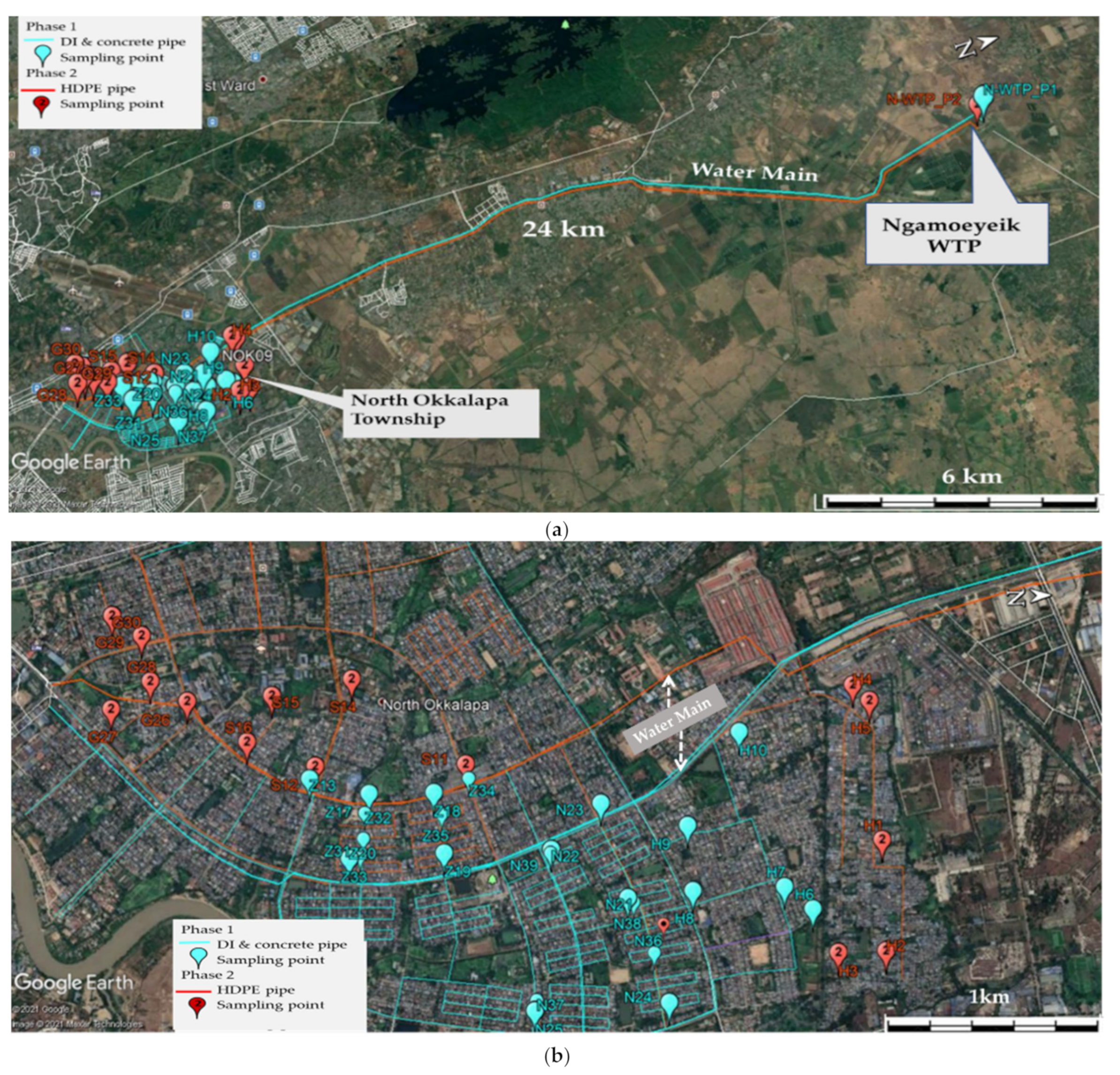
North Okkalapa Township (N-OKP, area 26.7 km2) is located in the Eastern District of Yangon City and is one of the largest townships in that area. N-OKP comprises 19 wards and has a population of 333,293 [28]. The distance from N-WTP to N- OKP is about 24 km (Figure 2a). N-WTP water is transmitted by Φ914 mm concrete pipes (Phase 1) and Φ1016 mm HDPE pipes (Phase 2). In 2019, it was calculated that there were 41,035 water supply connections and a service population of 308,896.
2.2. Field Sampling and Water Quality Analyses
Field sampling campaigns were conducted in N-WTP and N-OKP (Figure 2a,b) for the analysis of residual chlorine, chloroform as a representative species of THM, and other parameters listed in Table 3 and Table A1. N-WTP samples were taken from raw water, sedimentation tanks, and treated water tanks for Phase 1 and Phase 2 (Figure 1). Monitoring surveys were conducted twice: once in February 2020, when ACH was used as a coagulant, and once in December 2020, with PACl as a coagulant. In the N-OKP area (Figure 2b), 15 samples were taken from each of Phase 1 (3 from water mains and 12 from consumer taps) and Phase 2 (5 from water mains and 10 from consumer taps) water distribution networks in February 2020. In December 2020, 24 and 15 samples were taken from Phase 1 (4 from water mains and 20 from consumer taps) and Phase 2 (5 from water mains and 10 from consumer taps) networks, respectively; the increased number of the sampling points from 15 in February to 24 in December in Phase 1 was because of additional sampling points of Z31–Z35, N36–N39 (Figure 2b).
Both onsite sampling and laboratory analyses were carried out to assess the effectiveness of disinfection. Combined chlorine levels were calculated by subtracting free chlorine from total chlorine. SUVA indicates the level of aromatic substances—e.g., humic and fulvic acids—and was calculated from the ratio between UV254 absorbance and DOC by SUVA (L/mg-m) = UV254 × 100/DOC.
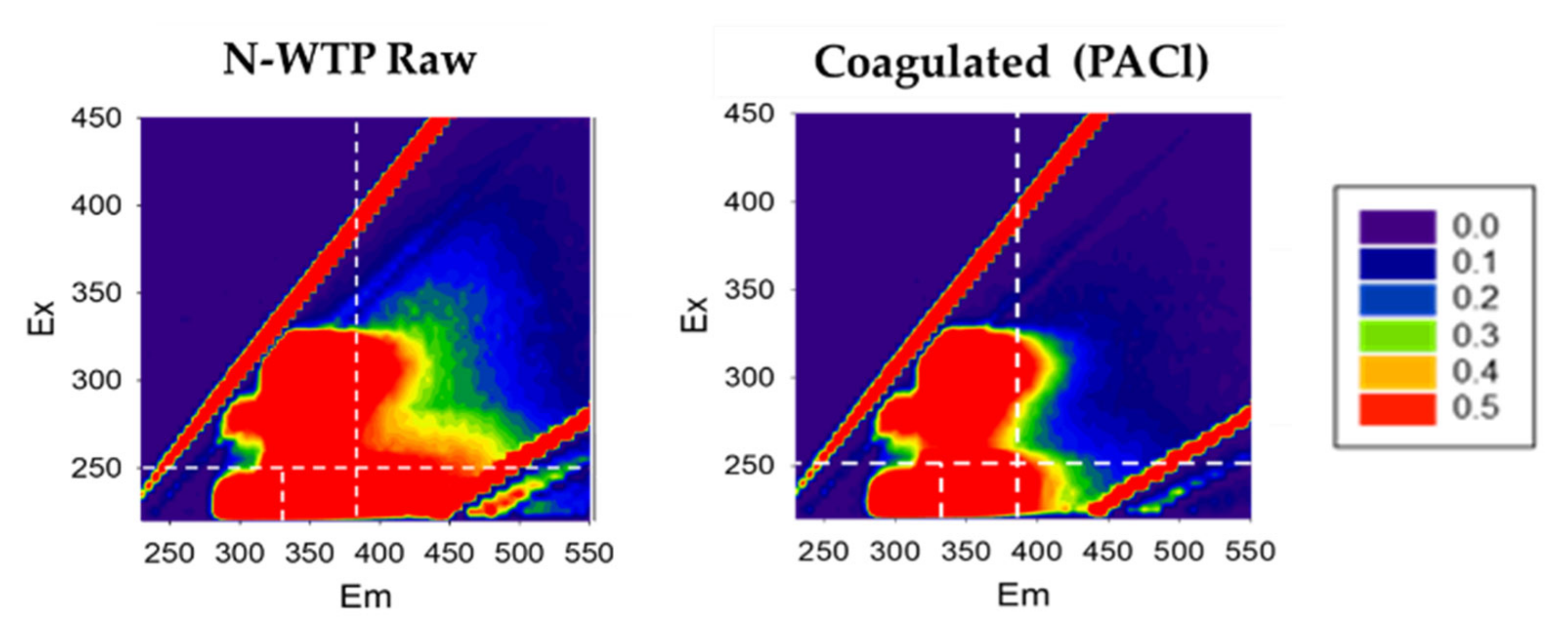
EEM was plotted using Sigma Plot 14.1 to obtain the fluorophores emitted by organic matter in water. EEM fluorophores are classified into five regions for the classification of organic matter: Region I (Ex. 250nm, Em. < 330 nm, tyrosine-like), II (Ex. < 250 nm, 330 nm < Em. < 380nm, tryptophan-like), III (Ex.< 250 nm, Em. >380nm, fulvic acid-like), IV (250 nm < Ex., Em. <380 nm, soluble microbial products), and V (Ex. >250 nm, Em. > 380 nm, humic acid -like) [29]. Among them, EEM regions III and V are good indicators of THM formation potential [11].
The value of total trihalomethanes (T-THM) was calculated by adding four THMs: chloroform, bromodichloromethane, dibromochloromethane, and bromoform. THMFP is the difference between the final and initial THM concentrations (THMFP = final T-THM–initial T-THM), while the level of initial THMs in raw water was close to zero and negligible [30]. Thus, THMFP is equal to the final T-THM concentration of the samples.
As it was difficult to analyze T-THM in Yangon due to the lack of GC-ECD in the analytical laboratory, only chloroform was analyzed in the water samples from N-WTP and N-OKP using THM plus (600 ppb, HACH, CO, USA). Then, T-THM was estimated by multiplying the chloroform concentration by the average ratio of T-THM/chloroform—i.e., 1.04—which was obtained in the THMFP experiments.
2.3. 24-h Monitoring of Residual Chlorine in Water Distribution Network
To find the variation in the residual chlorine in the distribution network, residual chlorine was monitored in the treated water tank of N-WTP and in the transmission mains at the N-OKP entry point for 24 h, with one-hour intervals between each measurement, in February 2020.
2.4. Chlorine Decay Tests
Batch chlorine decay tests were carried out at 23 °C by injecting sodium hypochlorite (NaClO) into coagulated N-WTP raw water. Coagulated raw water samples were prepared by mixing 25 mg/L of PACl with N-WTP raw water using a jar tester and settling for 30 min. Chlorine stock solution was prepared by diluting concentrated NaClO solution with Milli-Q water. The chlorine stock solution was added to the coagulated water samples in glass bottles to render the initial chlorine concentration 4 mg/L, which was determined to maintain the residual chlorine after 24 h at more than 1 mg/L. After the water samples were thoroughly mixed with the chlorine stock solution, the chlorine concentration was measured for 24 h at time intervals of every 20 min for the first 2 h and every hour after 2 h of reaction time. To analyze the chlorine decay in the water samples, first-order reaction models combining fast and slow reaction processes were applied to the data obtained in the chlorine decay tests.
2.5. Trihalomethane Formation Potential of Water Samples in the Water Treatment Plant
Trihalomethane formation potential (THMFP) was analyzed in water samples taken from the following points of the N-WTP: raw water, coagulated samples of raw water, and treated waters for Phases 1 and 2. The raw water samples were filtered through a glass fiber membrane filter (GF/F, 0.7µM, Whatman) to remove particulate matter. After membrane filtration, 10 mM of phosphate buffer solution (PBF) was added to control the pH to 7.0 ± 0.2. The chlorination of the samples was performed by adding sodium hypochlorite to the buffered samples, which were kept chlorine-free amber bottles (68.5 mL) without head space. Chlorine doses were determined to maintain 1 mg/L of residual free chlorine after 1 day of incubation to simulate the tap water residual free chlorine (Table 4). The treated water samples had already been chlorinated at N-WTP and re-chlorinated at the UT lab. Considering the water temperature and the hydraulic residence time of 3–7 h in Yangon, the samples were incubated at 25 °C for 1 day and 3 days before the THMFP measurements took place. For THM analysis, p-Bromo fluorobenzene was added as an internal standard. After the incubation period, the THM concentrations of the samples were determined using head space-gas chromatography with electron capture detection (GC-ECD, GC-2010 Plus, Shimadzu Co., Kyoto, Japan).
The average ratio of T-THM to chloroform was calculated from the above batch THMFP tests to estimate the T-THM from the chloroform measured in the water distribution network (refer to Section 2.2).
2.6. Data Analysis
Water quality data analysis was undertaken using R v.4.0.5. Box-and-whisker plots were used for the comparison of water quality in Phase 1 and Phase 2 of N-OKP. The Shapiro–Wilk test was used to determine normality, while t-test or non-parametric tests, such as the Wilcoxon test and Kruskal–Wallis test, were used to evaluate differences in the mean values of Phase 1 and Phase 2. The statistical tests were considered to be significant at p values less than 0.05.
2.7. Water Quality Simulation in the Networks
2.7.1. EPANET Network Model
The EPANET network simulation model allows water quality simulation in water distribution networks and has been widely applied to simulate residual disinfectants and DBPs in networks [31]. Thus, it was used to simulate the residual free chlorine concentration and THM formation in distribution networks in N-OKP and to determine the optimum—namely, the minimum adequate—chlorine dosage in N-WTP. The models simulate chlorine decay by assuming a constant chlorine concentration at the exit of N-WTP. In addition, the simulated and observed free chlorine concentrations were compared to check the accuracy of the model.
The water distribution network models for Phase 1 and Phase 2 in this study include only pipes greater than or equal to 110 mm in diameter and do not include service pipes with diameters smaller than 110 mm. The numbers of water demand nodes (junctions) were 124 and 53 in the Phase 1 and Phase 2 models, respectively. For hydraulic simulation, Hazen–Williams’s formula was employed with a roughness coefficient C of 140 because the ages of the supply pipes of ductile iron and concrete were over 16 years in Phase 1 and the HDPE was over 6 years old in Phase 2 [32].
2.7.2. Water Demand Allocation to Nodes
The water demand allocated to each node (junction) in the network was calculated from the water bills to the customers. As there is no previous study or data of water consumption variation for 24 h in Yangon City, the water demand pattern (Figure A1) was adopted from a previous study carried out in Bangkoknoi District, Bangkok, which has a high population density and a tropical climate similar to that of Yangon City [33].
2.7.3. Water Loss
Water loss was estimated from the difference between the water produced at N-WTP and the total water consumption in the N-WTP supply area. The estimated water losses were 46% and 40% in Phase 1 and Phase 2, respectively. However, there are no data on the location and amounts of water leakages; in addition, when we allocate the water loss evenly at all nodes, there are some nodes and pipelines with negative pressure, which halts the EPANET simulation. Thus, we conducted a simulation assuming no water loss, which provides higher values of THMs and chlorine decay due to the longer hydraulic retention times than the actual retention times with water leakages. Thus, if the simulation results could meet the guideline or target values of residual chlorine and THM concentrations at a certain chlorine dose, the actual values for residual chlorine and THMs concentration should also meet those values.
2.7.4. Reaction Coefficients
EPANET requires reaction rate equations and decay or growth rate coefficients to simulate the chemical species in a pipeline [34]. Chlorine decay is assumed to take place by two processes—bulk decay and wall decay—in distribution pipes.
Bulk Decay Coefficient (Kb)
Bulk chlorine decay refers to the reaction of chlorine with organic and inorganic constitutes in water. The laboratory batch chlorine decay test demonstrated that the chlorine decay reaction follows a two-step reaction—namely, fast and slow reaction processes (Figure A2). The bulk decay coefficient (Kb) of the EPANET models was selected as the slow reaction coefficient of 0.01 h−1 obtained in the batch chlorine decay tests because the hydraulic retention time in the treated water tanks was about 30 min, which is long enough to complete the fast reaction.
Wall Decay Coefficient (Kw)
The wall decay (Kw) refers to the reaction of chlorine with the pipe wall or the material accumulated on it in distribution systems [34]. The wall decay coefficient depends on the water temperature and the material, age, roughness, inner coating material, and biofilm formation of pipes. The first-order Kw values can range from 0 to 0.06 m/h [34]. Measuring the wall decay coefficient in laboratories is difficult and some researchers have assumed Kw based on previous studies [31]. As no measurement of the wall decay coefficient has been conducted in Yangon City, the wall coefficient Kw was assumed to be 0.02 h−1 for water mains based on the average values of 24 h monitoring data at the N-WTP-treated water tank and at the N-OKP inlet and 0.04 h−1 for pipes with diameters of 110 to 203 mm based on the monitoring data.
THM formation coefficient (k’)
Because it was not able to obtain the first-order THM formation coefficient by the batch THM formation tests, it was obtained as 0.008 h−1 by fitting the EPANET model outputs to the actual THM concentrations monitored at each node.
3. Results
3.1. Physical Parameters
Water temperatures were 27 ± 0.4 °C in the sampling period with ACH and 23 ± 0.5 °C in the sampling period with PACl at N-WTP and N-OKP. Figure 3a,b shows the pH in N-WTP and N-OKP, respectively. The pH values were within the range of the Myanmar National Drinking Water Quality Standards (hereafter MNDWQS) at both locations. The pH values of raw water, treated water, and tap water in N-OKP with PACl were significantly higher than those with ACH (Wilcoxon rank sum test, p < 0.05). However, there was no significant difference in pH values between Phase 1 and Phase 2 for both N-WTP and N-OKP (Wilcoxon rank sum test, p > 0.05).
As shown in Figure 3c,d, the turbidity reduction caused by PACl was more pronounced than that caused by ACH in N-WTP (Kruskal–Wallis test, p < 0.05). The mean values of raw water turbidity were 13 NTU and 14 NTU with ACH and PACl, respectively; these values were brought down by coagulation, sedimentation, and filtration to below 5 NTU in N-WTP. A significant difference in turbidity was observed between Phase 1 and Phase 2 in N-OKP (Kruskal–Wallis test, p < 0.05). These results indicate that no seasonal effect was observed because both February and December are in the dry winter season.
3.2. Chemical Parameters
3.2.1. Ammonia Nitrogen
Ammonia nitrogen was below 0.02 mg/L in raw water and not detected in treated and tap water.
3.2.2. Residual Chlorine
The residual chlorine data in N-WTP are shown in Figure 4a–c. The total chlorine concentrations in the Phase 1 sedimentation tank were about 1.5 mg/L and 1.3 mg/L for ACH and PACl, respectively, while the total chlorine concentrations in Phase 2 were 0.5 mg/L and 0.3 mg/L for ACH and PACl, respectively. The low chlorine concentrations in Phase 2 were due to the malfunctioning of the chlorine dosing pump of Phase 2 pre-chlorination during the sampling period. After post-chlorination, the treated water contained approximately 2.1 mg/L of total chlorine with ACH and PACl in Phase 1 and with ACH in Phase 2, but it was slightly less at 1.7 mg/L in Phase 2 PACl due to the above-mentioned malfunctioning of the pre-chlorination dosing pump. The difference in total chlorine concentrations between Phase 1 and Phase 2 was due to the difference in free chlorine concentrations because the combined chlorine was low at about 0.2 mg/L (Figure 4b,c).
In N-OKP (Figure 4d–f), the mean value of residual free chlorine was ca. 1.5 mg/L, while that of the combined chlorine was ca. 0.2 mg/L. No significant difference in total chlorine, free chlorine, and combined chlorine was found between Phase 1 and Phase 2 (Wilcoxon rank sum test, p > 0.05). The high residual free chlorine of ca. 1.5 mg/L at all the sampling points in N-OKP causes complaints about the noticeable chlorine smell from customers. Thus, it is necessary to reduce the residual chlorine concentration by decreasing the chlorine dose at the WTP.
3.2.3. Dissolved Organic Carbon (DOC)
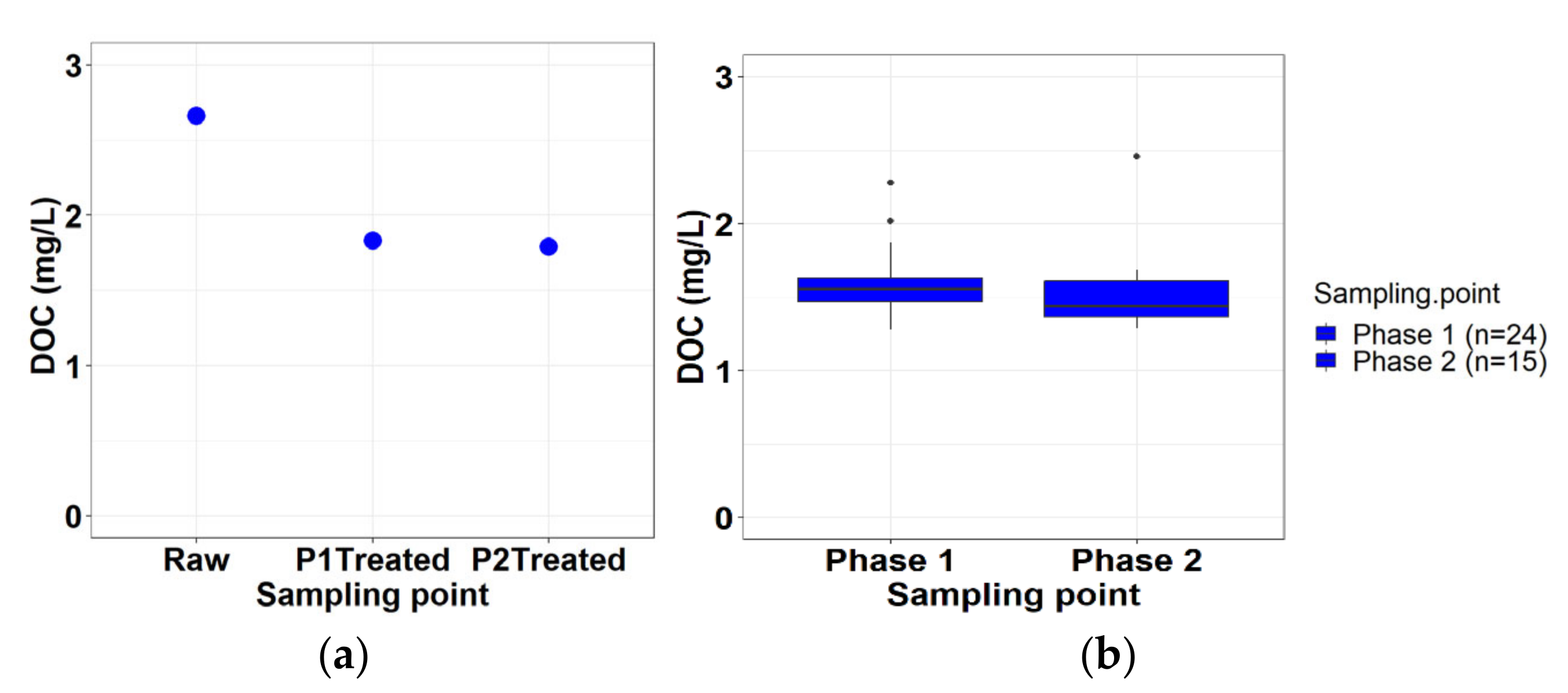
As shown in Figure 5a, the DOC of N-WTP raw water was approximately 2.8 mg/L at the sampling time when PACl was used as coagulant, and the treated waters contained ca. 2 mg/L of DOC in both the Phase 1 and Phase 2 processes. Thus, the removal rates of DOC were about 30% in both phases. DOC was slightly decreased to ca. 1.5 mg/L in the N-OKP distribution network (Figure 5b). There was also no significant difference in DOC concentration between Phase 1 and Phase 2 in N-OKP (Wilcoxon rank-sum test, p > 0.05).
3.2.4. UV254 Absorbance
The UV254 absorbance is an indicator of hydrophobic dissolved organic matter (DOM) and known to have a correlation with THMFP [19]. As shown in Figure 6, the UV254 of raw water was 0.045 and 0.039 cm−1 for the ACH and PACl processes, respectively; this was reduced to 0.015 and 0.021 cm−1 in the treated waters. This means that the reduction in UV254 was greater with ACH than with PACl. However, the UV254 in tap water increased to 0.020 cm−1 and 0.030 cm−1 with ACH and PACl, respectively, possibly due to the transformation of DOM and/or recontamination in the supply network. There was no significant difference between Phase 1 and Phase 2 in N-OKP (t- test, p > 0.05).
3.2.5. Specific Ultraviolet Absorbance (SUVA)
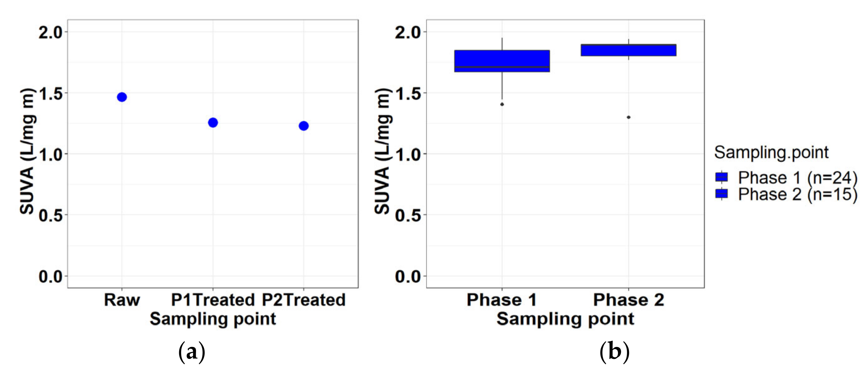
As shown in Figure 7, the SUVA of raw was ca. 1.5 L/mg-m, which was reduced to ca.1.3 L/min-m after PACl coagulation in N-WTP. The SUVA values increased from N-WTP to N-OKP in the supply network. Since DOC slightly decreased from N-WTP to N-OKP (Figure 5), it was estimated that the components of DOM were transformed to be more hydrophobic in the network. We found no significant difference in SUVA in N-OKP between Phase 1 and Phase 2 (Wilcoxon rank sum test, p >0.05).
3.2.6. Excitation Emission Matrix (EEM)
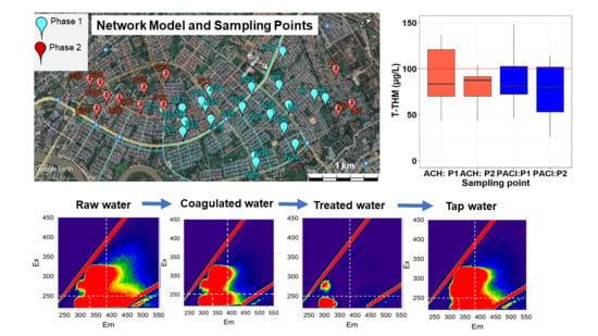
Figure 8 presents the EEM plots for the samples obtained at N-WTP and N-OKP along with the distance from N-WTP. Raw water contained significant amounts of soluble microbial products, aromatic proteins, and humic and fulvic acids. After coagulation, the levels of humic and fulvic acids were decreased. The EEM fluorophores in the treated waters in both Phase 1 and Phase 2 were significantly decreased from those in the coagulated samples, which indicated the effectiveness of organic matter removal by the filtration processes. Thus, the EEM was found to be a good analytical method for evaluating the DOM removal efficiency in the water treatment processes.
The water samples of N-OKP plotted in Figure 8 were selected from the household taps near the water mains in each ward of N-OKP. The EEM of Hta Ward, which is 19 km from N-WTP and located at the inlet of the N-OKP water main, showed small peaks of humic and fulvic materials. However, as the sampling location went farther from N-WTP, the fluorophores increased significantly in both Phase 1 (H10 to N23, and to Z19) and Phase 2 (H5 to S11, and to G26). Therefore, it was found that the EEM peaks intensified along with the pipeline length, which is in agreement with the increase in SUVA found in the supply network.
3.2.7. Trihalomethanes
The T-THM concentrations in N-WTP and in N-OKP are plotted in Figure 9a,b, respectively, along with the Drinking Water Quality Standard of Japan (100 µg/L), as there are no THM guideline values for MNDWQS. The T-THM concentrations were estimated from the chloroform concentration multiplied by 1.04, as described in the Materials and Methods section. They were 90 µg/L and 61 µg/L for Phase 1 and Phase 2 waters treated with ACH, respectively, and 78 µg/L and 85 µg/L for Phase 1 and Phase 2 water treated with PACl, respectively, at the N-WTP. The high variation in T-THM in treated waters might be due to changes in the raw water quality and unstable treatment efficiencies; however, the lower T-THM in ACH coagulated water in Phase 2 than in other samples was in agreement with the lower UV254 absorbance shown in Figure 6a.
There was no significant increase in the median values of tap water in the water distribution networks in N-OKP, although there were high variations among the sampling points. In particular, some samples taken at the end of the water distribution networks and away from the water mains contained over 100 µg/L of T-THM. There was no significant difference in the median THMs values between Phase 1 and Phase 2 in N-OKP (t-test, p >0.05), but Phase 1 ACH contained a higher ratio of samples with more than 100 µg/L of T-THM compared to Phase 1 PACl. More than three quarters—i.e., 75%—of the samples taken from the N-OKP network has below 100 µg/L for both Phases 1 and Phase 2 when PACl was used as a coagulant, but more than a quarter of the ACH samples were above 100 µg/L for Phase 1.
3.2.8. Trihalomethane Formation Potential (THMFP)
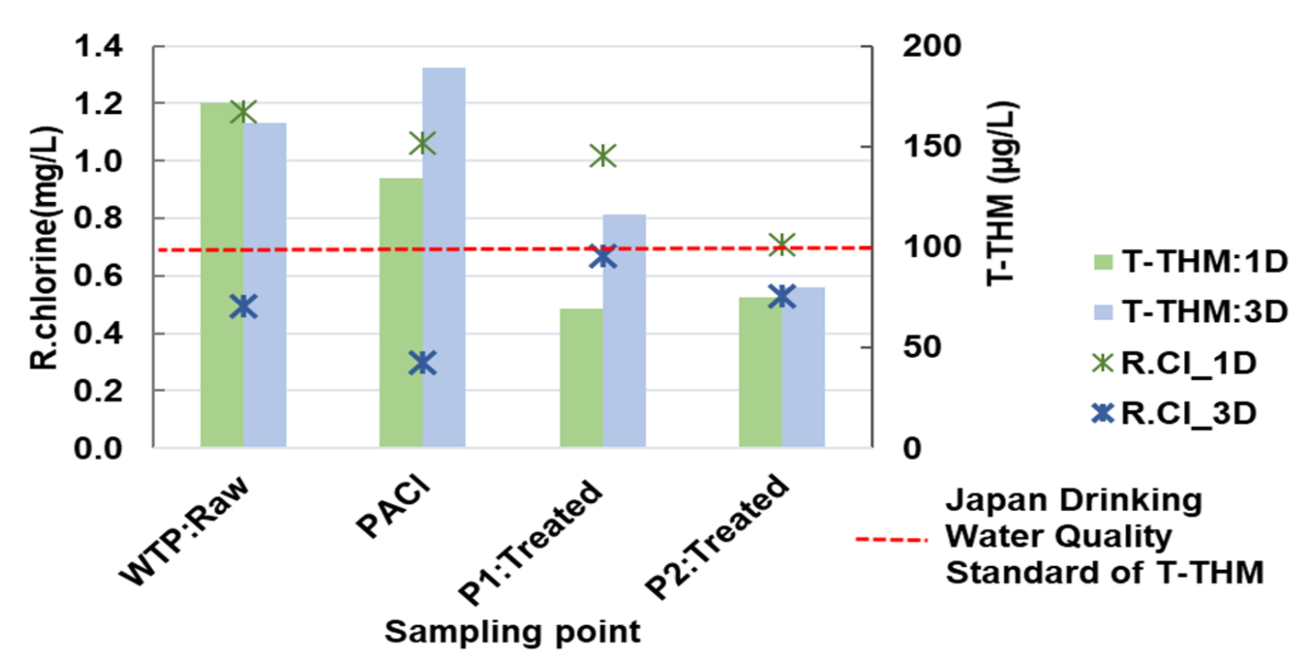
The THMFP values of the samples obtained at different points of N-WTP are shown in Figure 10. After the one-day incubation, the residual free chlorine was found to be approximately 1 mg/L in all samples. The T-THM concentrations were higher than 100 µg/L in the N-WTP raw and coagulated samples. The one-day THMFP values in the treated water were found to be ca. 70 µg/L, which is in agreement with the THM concentrations found in the treated water in the actual N-WTP. All the samples except the treated water from Phase 2 contained more than 100 µg/L (0.1 mg/L) T-THM after the 3-day incubation, which indicated a high level of THMFP in the raw water. Among the four constituents of T-THM, dibromochloromethane and bromoform were not detected in all samples because the bromide concentration was less than the detection limit of 0.1 mg/L in the raw water. The ratio of T-THM to chloroform was 1.04 for an average of 8 samples; this was used to estimate the T-THM from the chloroform concentration in the supply network samples.
3.2.9. 24-h Monitoring of Residual Chorine in the Networks
Figure 11a–d shows the total and free chlorine concentrations in the treated water at N-WTP and in water samples of the transmission mains taken at the inlet to N-OKP. The averages for total and free chlorine, indicated by dashed lines, were 2.0 mg/L and 1.8 mg/L, respectively, for both Phase 1 and Phase 2 at N-WTP. However, the measured chlorine concentration, especially the free chlorine concentration, varied more significantly in Phase 1 than in Phase 2, indicating the more stable operation of the Phase 2 water treatment process than the Phase 1 process. The free chlorine concentration dropped to ca. 1 mg/L at 6 a.m. and 8 a.m., respectively, in Phase 1, possibly due to chorine dose variations and/or errors caused by grab sampling. For instance, the added chlorine did not mix well with treated water due to the short retention time of about 30 min.
The total and free residual chlorine concentrations decreased to 1.5 mg/L and 1.3 mg/L, respectively, in N-OKP. As disinfected water contained organic matter and a high turbidity, residual chlorine decayed in reaction with these materials. Although there are a few peaks and drops of the total and free chlorine concentrations, they do not agree with the residual chlorine concentrations in N-WTP. Thus, those variations are considered to be caused by some problems of sampling and analysis.
3.3. Microbial Parameters
E. coli and total coliform were analyzed to evaluate the effectiveness of chlorine disinfection. Table 5 presents the results of the E.coli and total coliform analysis. Raw water contained 2400 and 2500 CFU/100 mL of E.coli and total coliform, respectively. Due to the high concentration of residual free chlorine in the water distribution networks, neither E. coli nor total coliform were detected in the treated waters and tap waters (n = 39). Thus, the disinfection performance was high enough to supply safe drinking water that was free of E. coli.
3.4. Water Quality Simulation in the Water Distribution Network
3.4.1. Residual Chlorine (Phase 1)
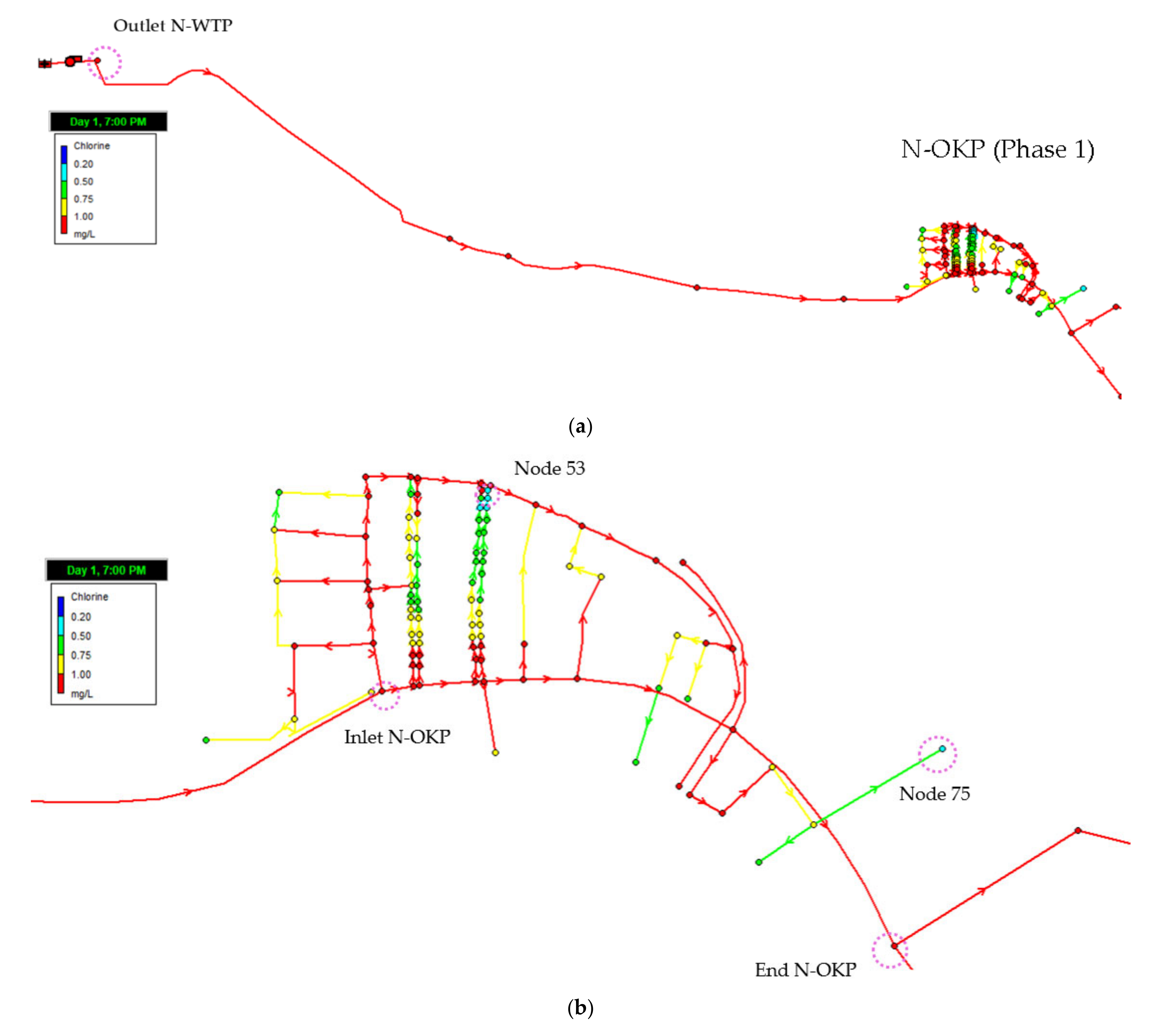
Figure 12a–c shows the simulation results, assuming a residual free chlorine concentration of 1.8 mg/L at the outlet from N-WTP, based on the mean value for the 24 h monitoring in N-WTP. The hydraulic retention time in the water mains from N-WTP to N-OKP is 7 h, and the residual chlorine concentrations were higher than 1 mg/L in most of the nodes (junctions), with the lowest concentration of ca. 0.4 mg/L found in small-diameter pipes in which the water flow velocities are low due to the small water demands. The measured and computed chlorine concentrations are correlated with small variations, as shown in Figure 12d. Such variations are caused by the difference between the actual and the model distribution networks, by the assumption of there being no water loss, and by the difference between the water sampling points and the nodes of the simulation models. For instance, the water samples were taken from the household taps, but the nodes were located on the distribution networks.
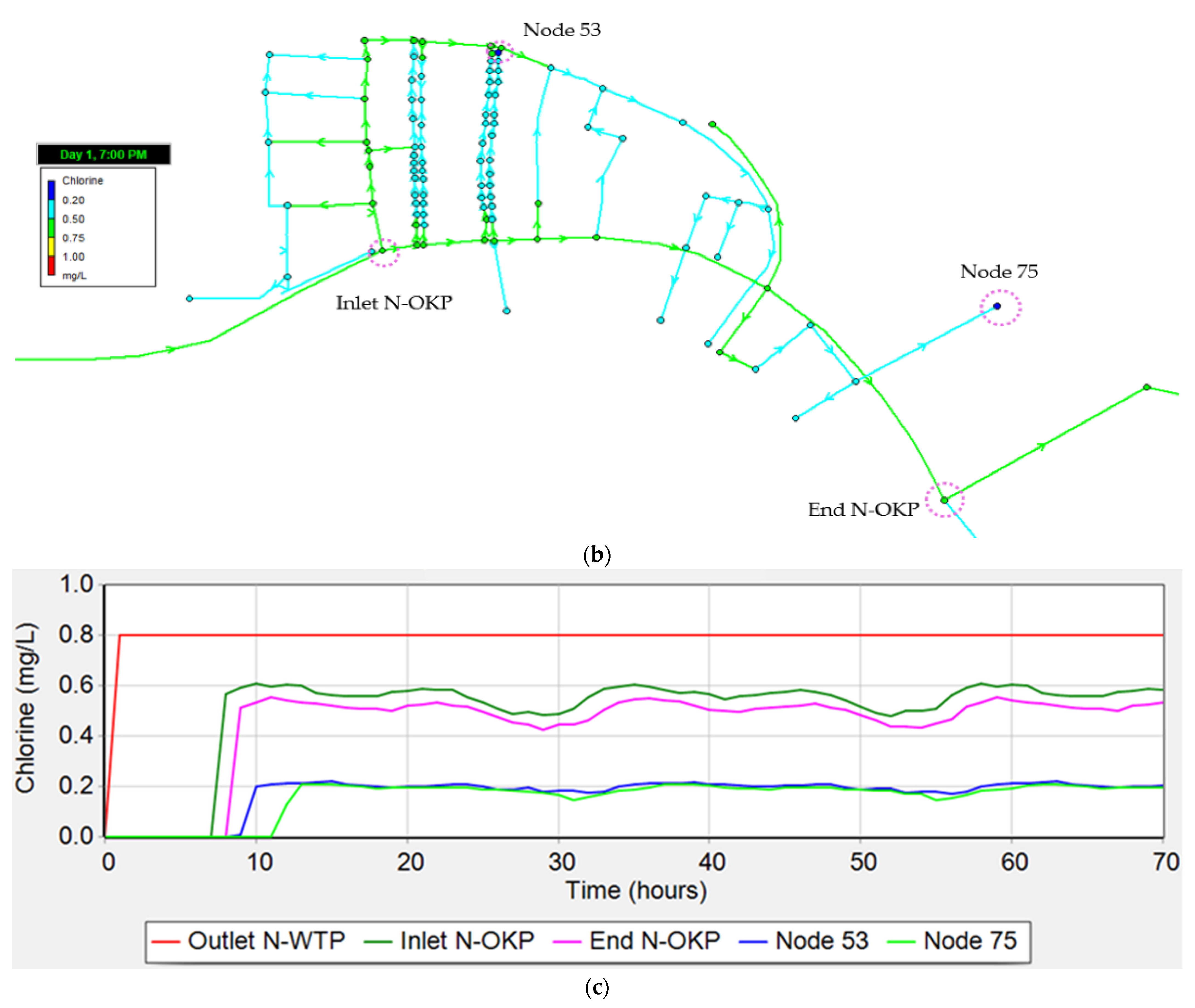
To find the lowest value for the residual free chlorine concentration at the outlet from N-WTP which can still maintain the minimum residual chlorine of 0.2 mg/L in the network, the residual free chlorine concentration at the outlet from N-WTP was gradually decreased from 1.8 mg/L; then it was found that 0.8 mg/L is sufficient to meet the residual free chlorine concentration of more than 0.2 mg/L at all nodes (Figure 13).
3.4.2. Trihalomethanes (Phase 1)
The THM formation simulation was carried out with the T-THM concentration of 78 µg/L at the outlet from N-WTP, which was the average of the monitoring data (Figure 9a, PACl). The simulation results showed that the T-THM concentration increased slightly to an average of 80 µg/L in the distribution network of N-OKP. The T-THM concentration of 60 µg/L at the outlet from N-WTP, which was assumed from the lowest T-THM concentration from Phase 2 with ACH, increased to 65 µg/L in the N-OKP network (Figure 14). Figure A3 and Table A2 in Appendix C compare the actual and simulated concentrations of T-THM. Although the median and mean values of the T-THM concentrations are similar between the actual and simulated results, there are high variations in the actual T-THM concentrations that was not reproduced by the simulation. These results indicate that there are unknown factors that cause variations in T-THM concentrations in the distribution network. The increase in SUVA values and EEM fluorophores indicates the transformation of DOM as a possible cause of T-THM formation in the network.
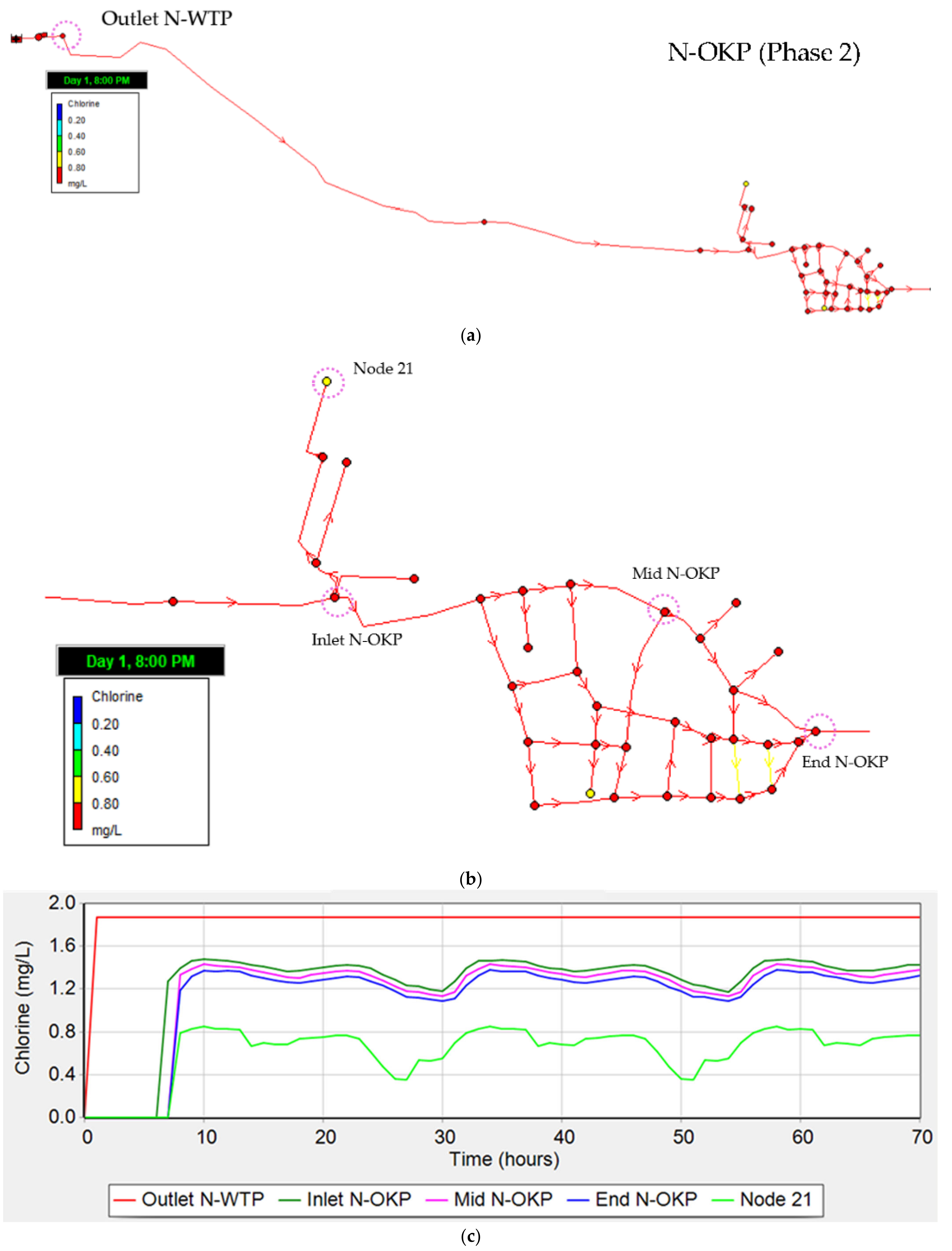
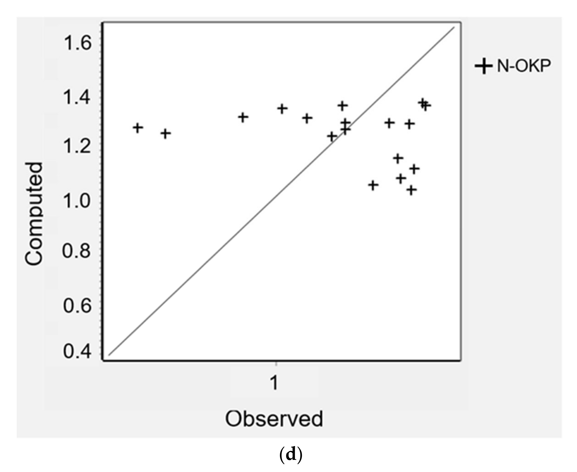
3.4.3. Residual Chlorine (Phase 2)
Figure A4a,b shows the distribution of chlorine concentration at all junctions in the Phase 2 distribution network. The hydraulic retention time in the transmission mains to N-OKP is 7 h and the residual free chlorine concentration is higher than 1 mg/L. As presented in Figure A4c, the simulated concentration and measured concentration of residual free chlorine are scattered below and above the diagonal line. Those points below the diagonal line are possibly caused by the longer hydraulic retention times due to the assumption of there being no water loss. Those above the diagonal line might be due to the difference in the sampling points and the nodes of the simulation model—for instance, the residual chlorine in taps could be lower than that in the distribution networks if there are long retention times in the service pipes or in the storage tanks. In the Phase 2 distribution network, however, it was found that the residual chlorine concentration at the outlet of N-WTP could be brought down to 0.7 mg/L to meet the target value of 0.2 mg/L (Figure A5).
3.4.4. Trihalomethanes (Phase 2)
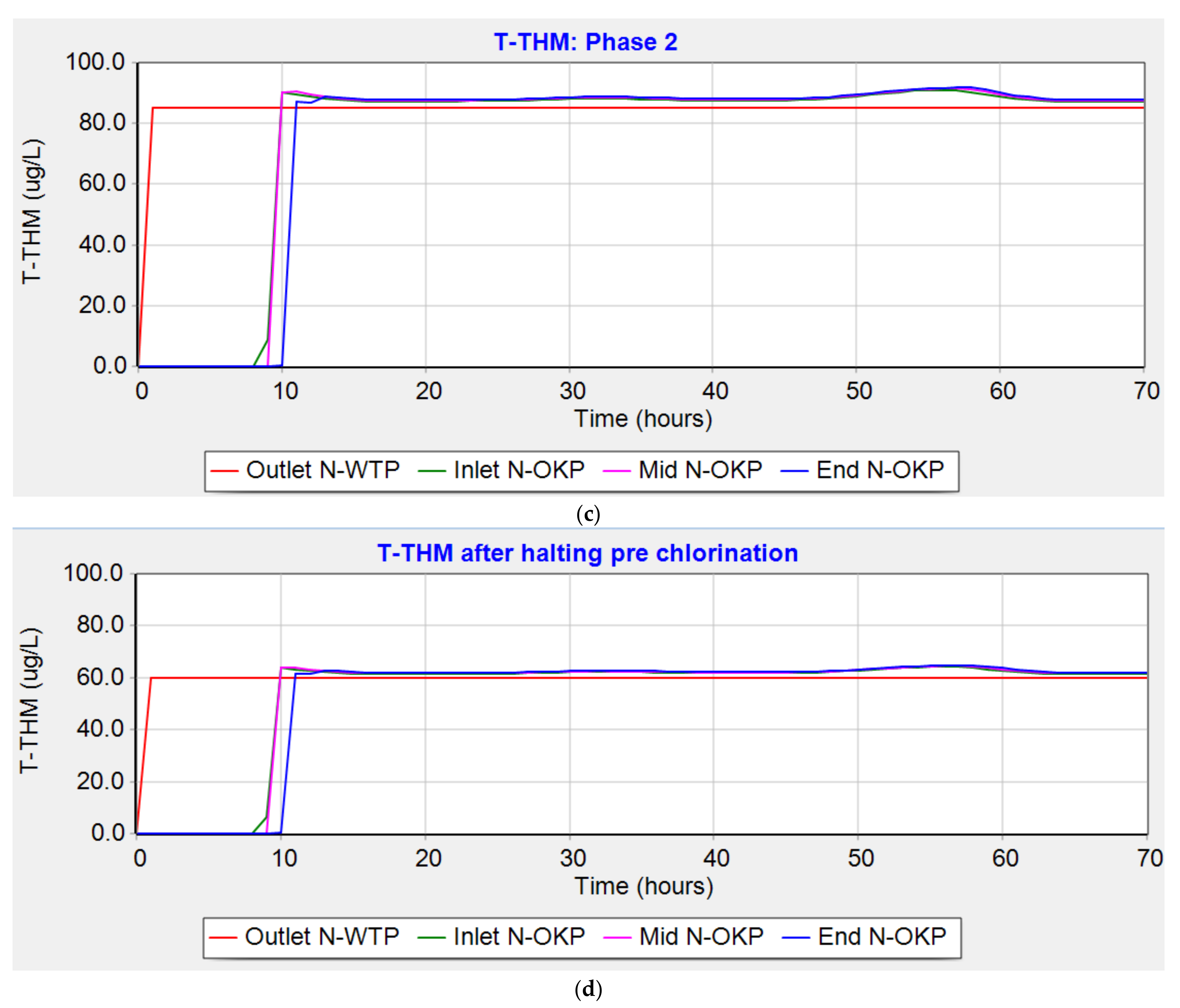
To simulate T-THM in the N-OKP network, the T-THM concentration at the outlet of N-WTP was set at two levels—i.e., a mean value of 85 µg/L in the monitoring and 60 µg/L assuming the lowest T-THM from Phase 2 ACH. The simulation results for the average T-THM in the N-OKP network are about 5 µg/L higher at 90 µg/L and 65 µg/L, respectively (Figure A6), due to THM formation in the networks.
4. Discussion
4.1. Effect of Changing Coagulant
N-WTP utilized ACH (17% Al2O3) at an injection concentration of 10 mg/L in the first sampling and PACl (30% Al2O3) at 18 mg/L in the second sampling. Thus, the aluminum concentration was increased from 1.9 to 5.5 mg/L. Therefore, the decreased turbidity observed after changing the coagulant from ACH to PACl is possibly due to an increased aluminum concentration [35].
In addition, the increased turbidity observed in the networks when ACH was used as coagulant might be due to re-suspension of particles deposited in the distribution pipes. As the ACH samples were taken just after chlorination started in January 2020, it is possible that the chlorine in water distribution pipes caused a slough-off of biofilm in the aged pipes and/or the resuspension of deposited particles. It might be reduced in the second sampling after 11 months of chlorination when PACl is used as the coagulant. Meanwhile, we found that changing the coagulant did not significantly influence other water quality parameters, including DOC removal, except that the UV254 absorbance and T-THM in the treated water were the lowest with Phase 2 ACH (Figure 6a and Figure 9a).
4.2. Water Quality Comparison between Phase 1 and Phase 2
The Phase 1 and Phase 2 processes of N-WTP employ the same treatment process and utilize the same amount of raw water. Although Phase 1 is about ten years older than Phase 2 and the filters are not so well designed and operated as in Phase 2, there was no statistically significant difference in water quality between Phase 1 and Phase 2 in the treated waters except for turbidity. Although in N-WTP the treated water turbidity was below the standard value of 5 NTU, it was higher than 1 NTU, which is the value required to maintain the effectiveness of chlorine disinfection [8].
The tap water turbidity found in Phase 1 was higher than the turbidity found in Phase 2 due to the poor filter performance at N-WTP, the different pipe materials used, namely concrete in Phase 1 vs. HDPE in Phase 2, and the different time of the samplings. Figure 15 shows the turbidity of the N-WTP-treated water (0 km) and the tap water samples in N-OKP along with the distance from N-WTP (19.0–21.5 km) with ACH and PACl. For both ACH and PACl, the Phase 1 turbidity was higher than the Phase 2 turbidity due to the poor performance of the Phase 1 filters. The turbidity increased along with the distance from N-WTP, except for the Phase 2 PACl. The turbidity increased in the distribution network due to sediment resuspension; the scouring of biofilms from the pipe walls of the aged pipes; and the oxidation of manganese, iron, and pipe metals [36]. The good operation of the water treatment processes and the good maintenance of the networks are important to meet the turbidity guideline value of 5 NTU at the taps.
The Phase 2-treated water contained residual chlorine in amounts almost the same as those of Phase 1 (Figure 4 and Figure 11), even though the chlorine dose was lower in the Phase 2 pre-chlorination at N-WTP, which indicates the possibility of reducing the pre-chlorination dose while maintaining a similar level of residual chlorine in the treated water. This may be partly due to the higher filtration efficiency of the Phase 2 process than the Phase 1 process.
Clark et al. observed that polyethylene pipes sustained a higher biofilm build-up than pipes made of cement, while a decreased level of DOC was found due to degradation by the microbes in the biofilm [37]. N-WTP supplied water without disinfection for 15 years through cement pipes (Phase 1) and for 5 years through HDPE pipes (Phase 2). Although no study of biofilm has been conducted in Yangon City, it is possible that the distribution pipes have biofilms due to there being no or only infrequent pipe cleaning. Thus, the decreased DOC in both Phase 1 and Phase 2 might also be due to biodegradation by the biofilm. Since SUVA, UV254, and EEM increased in the distribution network, it is likely that hydrophobic DOM was produced by microbial transformation in the supply network [38], which also increased the THMs in N-OKP [39,40].
4.3. Effect of Organic Matter on Chlorine Decay and THM Formation
High chlorine dosages due to high chlorine decay rates and high concentrations of dissolved organic matter in tropical countries cause high levels of THM formation [41,42]. Yangon is in a tropical region and the maximum water temperature was 30 °C in 2020, which was higher than the water temperature measured in this study. Thus, the effect of water temperature on chlorine decay and THM formation should be further investigated [19].
The chlorine decay processes of the N-WTP samples were found to be caused by a combination of two processes—namely, fast and slow reactions in the chlorine decay tests (Appendix B.2). The fast decay reaction takes place within 30 min, while the slow decay reaction takes a longer time. The fast-reacting components of organic matter produced a high THM concentration of about 140 µg/L in the THMFP tests, while the slow-reacting components showed no significant increase in the median values of THMs, except for a THM concentration variation at different sampling points (Figure 9). Moreover, the Phase 1 ACH samples in N-OKP had a higher ratio of samples containing over 100 µg/L of T-THM than Phase 1 PACl, which is in agreement with the higher turbidity found in Phase 1 PACl, indicating the effect of sampling just after chlorination commences.
The hydraulic retention time in the treated water tanks in N-WTP is 30 min, which is sufficient to complete the fast reaction of THM formation. Therefore, controlling THM formation in pre-chlorination processes is very important. This can be achieved by reducing the chlorine dose of, or by completely suspending, the pre-chlorination if the fast-reacting components of DOM can be effectively removed by coagulation–sand filtration processes. This is supported by the EEM results; high concentrations of humic and fulvic-like components were effectively removed by Phase 1 and Phase 2 coagulation–sand filtration, as reported by previous studies [5,43].
According to the THMFP experimental results (Figure 10), the THM formation decreased almost by half from ca. 140 µg/L in raw water to ca. 70 µg/L in treated water in both the Phase 1 and Phase 2 processes. This is in agreement with the UV absorbance reduction from 0.040–0.046 to 0.020–0.023 (Figure 6). Thus, if we halt pre-chlorination, it may be possible to reduce the THMFP to less than 70 µg/L due to a short hydraulic retention time of 30 min compared to using one day of THMFP tests. Although pre-chlorination has several effects, such as oxidizing iron and manganese and preventing algal growth in clarifiers, these problems had not been reported before the chlorination systems commenced operation in January 2020. However, it is recommended, during the practical operation of chlorination systems, that the chlorine dose used in pre-chlorination should be gradually reduced to the lowest possible dose. It is also advised that the chlorine dose used in post-chlorination is also to be brought down from 2 mg/L. To do so, it is very important to maintain a high DOM removal efficiency in the N-WTP.
4.4. Water Distribution Network Modelling
In the simulation of water flow and water quality in the distribution network of Yangon City, there are limitations in the availability of the input data for the networks and water quality because of the obsoleteness of the network data and the lack of regular monitoring of residual chlorine and THMs in the N-WTP and N-OKP. The water sampling points were household taps for residual chlorine and THM analysis, but in the simulation models, the water quality was plotted at the nodes of the distribution networks. As there was no water consumption pattern monitoring in Yangon City, the water demand pattern from Bangkoknoi District, Bangkok, was adopted, which might be different from the actual water demand pattern of Yangon City.
Unlike the low water loss of less than 20% that can be expected in well-maintained water distribution systems [44], the high water loss in Yangon City of 40–46% made the network simulation difficult to run using EPANET. Thus, the network simulation model was run assuming no water loss, which provides higher values for THMs and chlorine decay rates than the actual values due to the longer hydraulic retention times in the networks. These limitations of the simulation model made it difficult to predict the water quality with a high accuracy and caused a high variation in the water quality data among the samples from the taps.
The chlorine decay in the simulation was more pronounced than that in the actual network, especially at the dead-end nodes due to the hydraulic retention times being longer than the actual ones, as the simulation models were run without water loss. In addition, dead-end junctions could be connected to other pipes in the actual network that are not recorded on the network map. Although these limitations and errors make the accurate simulation of the actual water quality impossible, the simulation results err on the safer side for both THMs and residual chlorine estimation; therefore, the lowest chlorine dose that complies with both residual chlorine and T-THM guidelines in the simulation model could be applied to the chlorine dose in the practical operation of these chlorination systems.
5. Conclusions
Yangon City has supplied water for many years without adequate chlorination. Thus, it is difficult to optimize the chlorine dose to minimize THMs in the networks while maintaining the minimum concentration of residual free chlorine. This study presented and verified the effectiveness of the method of combining the field monitoring of water quality, batch chlorine decay tests, and THM formation experiments with water quality simulation in the network to optimize the chlorine dose.
Although the turbidity removal efficiency in N-WTP was low, the turbidity in treated waters was less than 5 NTU for the coagulants of ACH and PACl. However, the turbidity in tap waters was higher than that in the treated water of N-WTP due to the poor maintenance of the pipe networks. Thus, the good maintenance of water supply pipes is needed to avoid water quality deterioration in the network.
Due to the high chlorine dose of 2 mg/L for pre- and post-chlorination in N-WTP, the residual chlorine in the treated and tap water was high at ca. 1.5 mg/L, causing customers to complain about the chlorine smell and high level of THMs. The batch chlorine decay tests revealed that the raw water contained two DOM components that had fast and slow reactions with chlorine. As pre-chlorination brings about chlorine reactions with fast-reacting DOM and the formation of high levels of THMs, pre-chlorination should be significantly curtailed to lower the THM concentration in treated water. On the other hand, the chlorine decay and THM formation in the supply networks were not significant because of the reaction with the slow-reacting DOM. Based on the THMFP experiments, it was estimated that, by improving the treatment efficiency of coagulation and sand filtration processes, it would be possible to reduce the chlorine dose to minimize THM formation.
The DOC removal rates at N-WTP were ca. 30% and the SUVA was slightly decreased, indicating the higher removal of the hydrophobic fraction than the hydrophilic fraction. Decreased DOC was found in tap water, possibly because of DOC degradation due to biofilms and the adsorption on pipe materials in the networks. Furthermore, the EEM was found to be a sensitive and useful tool for monitoring DOC removal in water treatment plants and for the transformation of DOM in piped water. The increased fluorophores of EEM along with the water distribution pipes indicated the transformation of DOM within the pipes.
Water quality simulation in the network was conducted, assuming there to be no water loss to find the minimum dose of chlorine that meets the guidelines for both THMs and residual chlorine concentrations. As a result of water quality simulation combined with batch chlorine decay and THM formation tests, it was found that controlling the chlorine and THM concentration at the outlet of the water treatment plant is critical to minimize the chlorine dose while meeting the target values for residual chlorine and THMs in the distribution network. Although chlorine decay was found in small-diameter pipes, THMs did not significantly increase in distribution network. It is difficult to reproduce the T-THM variation in the networks because the causes of such variations have not yet been identified.
A combination of field monitoring, batch chlorine decay and THMFP tests, and the network simulation in this study made it possible to find the cause of high THMs concentration in distributed water and the minimum chlorine dose to meet the guideline values for the residual chlorine and THMs, even in a water supply system with limited available data. Thus, the methods employed in this study would also be useful for other water supply systems in developing countries where data on distribution networks and water quality are limited and the water loss is as high as in Yangon City.
Author Contributions
Conceptualization, S.T., N.N.Z. and S.K.; methodology, S.K. and S.T.; data analysis, N.N.Z., S.K. and S.T.; investigation, N.N.Z.; data curation, N.N.Z. and S.K.; writing—original draft preparation, N.N.Z.; writing—review and editing, S.T. and S.K.; visualization, N.N.Z.; supervision, S.T. and S.K.; project administration, S.K. and S.T.; funding acquisition, S.T. All authors have read and agreed to the published version of the manuscript.
Funding
This research was funded by Japan International Cooperation Agency (JICA) though the collaborative program with the University of Tokyo and the scholarship provided to Nwe Nwe Zin for her graduate studies.
Institutional Review Board Statement
Not applicable.
Informed Consent Statement
Not applicable.
Data Availability Statement
Not applicable.
Acknowledgments
The authors would like to express their gratitude to Water Resources and Water Supply Authority, Yangon City Development Committee (YCDC).
Conflicts of Interest
The authors declare no conflict of interest.
Appendix A

Table A1.
Equipment for water quality analysis.
| No. | Parameters | Equipment |
|---|---|---|
| 1 | pH, Temperature | LAQUAact, Horiba, Kyoto, Japan |
| 2 | Turbidity | Thermo Scientific TN-100, Thermo Scientific Eutech Instruments Pre Ltd., Singapore |
| 3 | Residual chlorine | DR 890 HACH Potable Colorimeter, HACH, CO, USA |
| 4 | Ammonia- nitrogen | |
| 5 | Trihalomethanes (Chloroform) | DR 6000 HACH Spectrophotometer, CO, USA |
| 6 | Trihalomethanes | Shimadzu GC-2010 Plus, Kyoto, Japan |
| 7 | UV254 Absorbance | UH-5300, Hitachi High-Tech Science Co., Tokyo, Japan |
| 8 | Dissolved Organic Carbon | TOC-L analyzer, Shimadzu, Kyoto, Japan |
| 9 | Excitation Emission Matrix (EEM) | Agilent Cray Eclipse Fluorescence Spectrophotometer, CA, USA |
| 10 | Bromide | Metrohm 861 Advance Compact IC, Metrohm, Herisau, Switzerland |
Appendix B
Appendix B.1. Water Demand Pattern
Figure A1.
Water demand pattern [33].
Figure A1.
Water demand pattern [33].

Appendix B.2. Batch Decay Tests of Chlorine
The chlorine concentrations measured in the batch chlorine decay tests were fitted with Equations (A1) and (A2), as shown in Figure A2. Assuming the chlorine to dissolved organic matter (DOM) ratio to be 1, the fast reaction coefficient at 0.02 h−1 and the slow reaction coefficient at 0.01 h−1 gave the best fit for the actual and the model residual concentration. As the retention time in the N-WTP is 30–40 min, the slow reaction coefficient of 0.01h−1 was employed as a bulk decay coefficient in the water distribution network.
where C is the residual chlorine concentration at time t; S is organic matter at time t; Sf is the fast-reacting components of organic matter at time t; a is the reaction ratio of organic matter to chlorine; and kf and ks are the fast and slow reaction coefficients, respectively.
Figure A2.
Reduction in chlorine and DOM.

Appendix C
Figure A3.
THMs in N-OKP and computed T-THM in EPANET: (a) Phase 1, (b) Phase 2.

Table A2.
THMs in N-OKP and computed in EPANET.
| Phase 1 | Phase2 | |||||
|---|---|---|---|---|---|---|
| ACH: P1 (n = 15) | PACl:P1 (n = 24) | Computed (n = 99) | ACH: P2 (n = 15) | PACl:P2 (n = 15) | Computed (n = 33) | |
| Standard deviation (SD) | 35 | 27 | 0 | 25 | 34 | 1 |
| Mean | 99 | 88 | 79 | 99 | 82 | 84 |
| Minimum | 43 | 43 | 78 | 66 | 26 | 82 |
| Maximum | 167 | 169 | 79 | 148 | 151 | 86 |
Figure A3 presents the T-THM variation in N-OKP and the results computed by EPANET for Phase 1 and 2. Although the T-THM in N-OKP showed a high variation, the computed results did not have a high variation. The EPANET model results were not increased significantly in either Phase 1 or Phase 2. However, the mean values of THMs with PACl were close to the computed results by EPANET.
Appendix D
Figure A4.
Simulation of chlorine in Phase 2 (N-WTP outlet: 1.9 mg/L): (a) network model, (b) residual chlorine in N-OKP, (c) time course of chlorine concentration, and (d) observed vs. simulated chlorine.
Figure A4.
Simulation of chlorine in Phase 2 (N-WTP outlet: 1.9 mg/L): (a) network model, (b) residual chlorine in N-OKP, (c) time course of chlorine concentration, and (d) observed vs. simulated chlorine.


Figure A5.
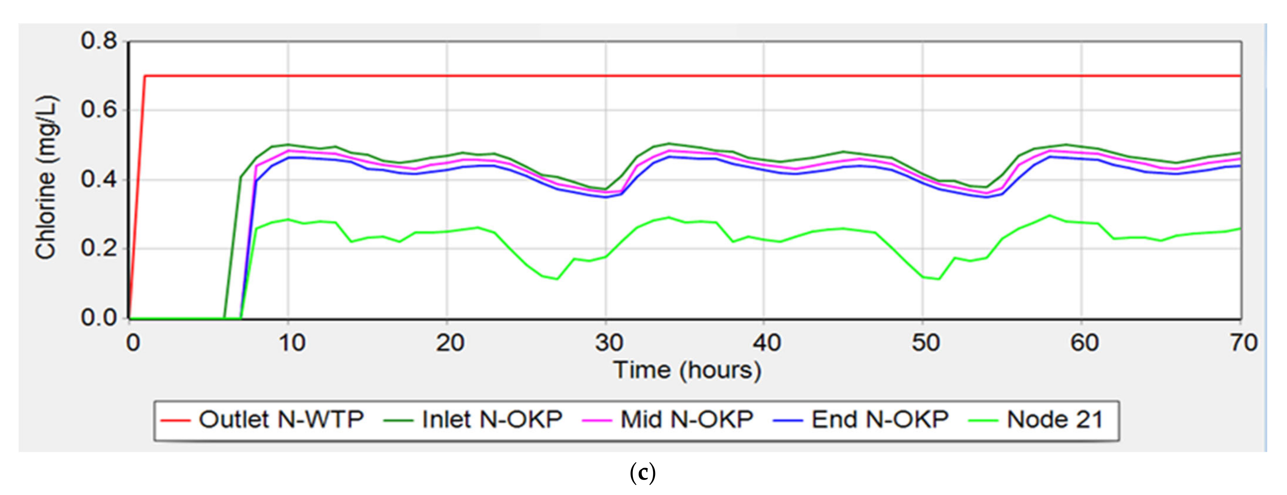
Simulation of chlorine in Phase 2 (initial chlorine 0.7 mg/L): (a) Phase 2 model, (b) chlorine in N-OKP, and (c) chlorine concentration in model.
Figure A5.
Simulation of chlorine in Phase 2 (initial chlorine 0.7 mg/L): (a) Phase 2 model, (b) chlorine in N-OKP, and (c) chlorine concentration in model.


Figure A6.
Simulation of trihalomethanes in Phase 2: (a) T-THM model; (b) T-THM in N-OKP area; (c) T-THM concentration with initial T-THM for treated water: 85 µg/L; (d) T-THM concentration in model after halting pre-chlorination: 60 µg/L.
Figure A6.
Simulation of trihalomethanes in Phase 2: (a) T-THM model; (b) T-THM in N-OKP area; (c) T-THM concentration with initial T-THM for treated water: 85 µg/L; (d) T-THM concentration in model after halting pre-chlorination: 60 µg/L.


References
- Nieuwenhuijsen, M.; Toledano, M.; Eaton, N.; Fawell, J.; Elliott, P. Chlorination disinfection byproducts in water and their association with adverse reproductive outcomes. Occup. Environ. Med. 2000, 57, 73–85. [Google Scholar] [CrossRef] [PubMed] [Green Version]
- Mostafa, N.; Matta, M.; Abdel-Halim, H. Simulation of Chlorine Decay in Water Distribution Networks Using EPANET–Case Study. Civ. Environ. Res. 2013, 3, 100–116. [Google Scholar]
- Jonkergouw, P.M.R.; Khu, S.-T.; Savic, D.A.; Zhong, D.; Hou, X.Q.; Zhao, H.-B. A Variable Rate Coefficient Chlorine Decay Model. Environ. Sci. Technol. 2009, 43, 408–414. [Google Scholar] [CrossRef] [PubMed]
- Clark, R.; Sivagansen, M. Predicting Chlorine Residuals and the Formation of T-THM in Drinking Water. J. Environ. Eng. 1998, 124, 1203–1210. [Google Scholar] [CrossRef]
- Gang, D.C.; Clevenger, T.E.; Banerji, S.K. Modeling Chlorine Decay in Surface Water. J. Environ. Inform. 2015, 1, 21–27. [Google Scholar] [CrossRef]
- WHO. World Health Organization, Guidelines for Drinking Water Quality, 3rd ed.; WHO: Geneva, Switzerland, 2008; Volume 1, pp. 451–454. Available online: https://www.who.int/water_sanitation_health/dwq/fulltext.pdf (accessed on 2 July 2021).
- Richardson, S.; Plewa, M.; Wagner, E.; Schoeny, R.; Demarini, D. Occurrence, Genotoxicity, and Carcinogenicity of Regulated and Emerging Disinfection Byproducts in Drinking Water: A Review and Roadmap for Research. Mutat. Res. Rev. Mutat. Res. 2007, 636, 178–242. [Google Scholar] [CrossRef]
- Environmental Protection Agency. Water Treatment Manual: Disinfection. 2011. Available online: https://www.epa.ie/publications/compliance--enforcement/drinking-water/advice--guidance/Disinfection2_web.pdf (accessed on 28 April 2021).
- Ministry of Health Labour and Welfare (MHLW), Japan, Drinking Water Quality Standard. 2012. Available online: https://www.mhlw.go.jp/english/policy/health/water_supply/dl/4a.pdf (accessed on 15 May 2021).
- Japan Water Works Association (JWWA). Water Treatment Facilities of the Design Criteria for Water Supply Facilities. 2012. Available online: https://www.mhlw.go.jp/file/06-Seisakujouhou-10900000-Kenkoukyoku/0000103931.pdf (accessed on 14 April 2021).
- Sakai, H.; Tokuhara, S.; Murakami, M.; Kosaka, K.; Oguma, K.; Takizawa, S. Comparison of Chlorination and Chloramination in Carbonaceous and Nitrogenous Disinfection Byproduct Formation Potentials with Prolonged Contact Time. Water Res. 2016, 88, 661–670. [Google Scholar] [CrossRef]
- Rakruam, P.; Wattanachira, S. Reduction of DOM Fractions and Their Trihalomethane Formation Potential in Surface River Water by In-Line Coagulation with Ceramic Membrane Filtration. J. Environ. Sci. 2014, 26, 529–536. [Google Scholar] [CrossRef]
- Musikavong, C.; Wattanachira, S. Identification of Dissolved Organic Matter in Raw Water Supply from Reservoirs and Canals as Precursors to Trihalomethanes Formation. J. Environ. Sci. Health Part A 2013, 48, 760–771. [Google Scholar] [CrossRef]
- Lundqvist, J.; Andersson, A.; Johannisson, A.; Lavonen, E.; Mandava, G.; Kylin, H.; Bastviken, D.; Oskarsson, A. Innovative Drinking Water Treatment Techniques Reduce the Disinfection-Induced Oxidative Stress and Genotoxic Activity. Water Res. 2019, 155, 182–192. [Google Scholar] [CrossRef]
- Zhao, Y.; Xiao, F.; Wang, D.; Yan, M.; Bi, Z. Disinfection Byproduct Precursor Removal by Enhanced Coagulation and Their Distribution in Chemical Fractions. J. Environ. Sci. 2013, 25, 2207–2213. [Google Scholar] [CrossRef]
- Amarasooriya, A.A.G.D.; Weragoda, S.; Makehelwala, M.; Weerasooriya, R. Occurrence of Trihalomethane in Relation to Treatment Technologies and Water Quality under Tropical Conditions. H2Open J. 2018, 1. [Google Scholar] [CrossRef] [Green Version]
- Valdivia-Garcia, M.; Weir, P.; Graham, D.; Werner, D. Predicted Impact of Climate Change on Trihalomethanes Formation in Drinking Water Treatment. Sci. Rep. 2019, 9. [Google Scholar] [CrossRef] [PubMed]
- Delpla, I.; Jung, A.-V.; Baurès, E.; Clement, M.; Thomas, O. Impacts of Climate Change on Surface Water Quality in Relation to Drinking Water Production. Environ. Int. 2009, 35, 1225–1233. [Google Scholar] [CrossRef] [PubMed]
- Phetrak, A.; Lohwacharin, J.; Takizawa, S. Analysis of Trihalomethane Precursor Removal from Sub-Tropical Reservoir Waters by a Magnetic Ion Exchange Resin Using a Combined Method of Chloride Concentration Variation and Surrogate Organic Molecules. Sci. Total Environ. 2016, 539, 165–174. [Google Scholar] [CrossRef] [Green Version]
- Osawa, H.; Lohwacharin, J.; Takizawa, S. Controlling Disinfection By-Products and Organic Fouling by Integrated Ferrihydrite–Microfiltration Process for Surface Water Treatment. Sep. Purif. Technol. 2017, 176, 184–192. [Google Scholar] [CrossRef]
- Momba, M.; Kfir, R.; Venter, S.; Cloete, T. An Overview of Biofilm Formation in Distribution Systems and Its Impact on the Deterioration of Water Quality. Water SA 2000, 26, 59–66. Available online: http://hdl.handle.net/10204/742 (accessed on 28 April 2021).
- Ding, S.; Deng, Y.; Bond, T.; Fang, C.; Cao, Z.; Chu, W. Disinfection Byproduct Formation during Drinking Water Treatment and Distribution: A Review of Unintended Effects of Engineering Agents and Materials. Water Res. 2019, 160, 313–329. [Google Scholar] [CrossRef] [PubMed]
- Liu, G.; Zhang, Y.; Knibbe, W.-J.; Feng, C.; Liu, W.; Medema, G.; van der Meer, W. Potential Impacts of Changing Supply-Water Quality on Drinking Water Distribution: A Review. Water Res. 2017, 116, 135–148. [Google Scholar] [CrossRef]
- Karaderek, I.E.; Kara, S.; Muhammetoglu, A.; Muhammetoglu, H.; Soyupak, S. Management of chlorine dosing rates in urban water distribution networks using online continuous monitoring and modeling. Urban Water J. 2016, 13, 245–359. [Google Scholar] [CrossRef]
- JICA, A Strategic Urban Development Plan of Greater Yangon Final Report 1, April 2013. Available online: https://openjicareport.jica.go.jp/pdf/12122511.pdf (accessed on 19 March 2021).
- AWWA, Water Treatment Plant Design, Fourth Edition. 2004. Available online: https://www.academia.edu/25857768/Water_Treatment_Plant_Design_4th_Edition (accessed on 25 May 2021).
- Yangon City Development Committee. Research Report of Filter Improvement Task Force Team; Yangon City Development Committee (YCDC): Yangon, Myanmar, 2019.
- Ministry of Labour, Immigration and Population, The 2014 Myanmar Population and Housing Census, Yangon Region, Eastern District, North Okkalapa Township Report, October 2017. Available online: https://themimu.info/sites/themimu.info/files/documents/TspProfiles_Census_NorthOkkalapa_2014_ENG.pdf (accessed on 25 September 2020).
- Chen, W.; Westerhoff, P.; Leenheer, J.A.; Booksh, K. Fluorescence Excitation−Emission Matrix Regional Integration to Quantify Spectra for Dissolved Organic Matter. Environ. Sci. Technol. 2003, 37, 5701–5710. [Google Scholar] [CrossRef] [PubMed]
- APHA. Standard Methods for the Examination of Water and Waste Water, 23rd ed.; American Public Health Association: Washington, DC, USA, 2017; pp. 5–70. [Google Scholar]
- Sorlini, S.; Biasibetti, M.; Gialdini, F.; Muraca, A. Modeling and Analysis of Chlorine Dioxide, Chlorite, and Chlorate Propagation in a Drinking Water Distribution System. J. Water Supply Res. Technol.-Aqua 2016, 65, 597–611. [Google Scholar] [CrossRef]
- Viessman, W. The Water Supply and Pollution Control, 8th ed.; Pearson: New York, NY, USA, 2008; pp. 126–191. [Google Scholar]
- Islam, M.S. Leakage Analysis and Management in the Water Distribution Network in a Selected Area of Bangkok. Master’s Thesis, Asian Institute of Technology, Khlong Nueng, Thailand, 2005. [Google Scholar]
- Rossman, L.A. EPANET 2 User’s Manual. 2000. Available online: https://www.microimages.com/documentation/Tutorials/Epanet2UserManual.pdf (accessed on 27 April 2021).
- Zhao, H.; Hu, C.; Liu, H.; Zhao, X.; Qu, J. Role of Aluminum Speciation in the Removal of Disinfection Byproduct Precursors by a Coagulation Process. Environ. Sci. Technol. 2008, 42, 5752–5758. [Google Scholar] [CrossRef] [PubMed]
- Mohammed, H.; Tornyeviadzi, H.M.; Seidu, R. Modelling the Impact of Water Temperature, Pipe, and Hydraulic Conditions on Water Quality in Water Distribution Networks. Water Pract. Technol. 2021, 16, 387–403. [Google Scholar] [CrossRef]
- Clark, R.; Lykins, B.; Block, J.C.; Wymer, L.; Reasoner, D. Water Quality Changes in a simulated distribution system. J. Water Supply: Res. Technol.-Aqua 1994, 43, 263–277. [Google Scholar] [CrossRef]
- Chen, J.; Gu, B.; Leboeuf, E.; Pan, H.; Dai, S. Spectroscopic Characterization of Structural and Functional Properties of Natural Organic Matter Fractions. Chemosphere 2002, 48, 59–68. [Google Scholar] [CrossRef]
- Jung, C.-W.; Son, H.-J. The Relationship between Disinfection By-Products Formation and Characteristics of Natural Organic Matter in Raw Water. Korean J. Chem. Eng. 2008, 25, 714–720. [Google Scholar] [CrossRef]
- Singer, P.C. Humic Substances as Precursors for Potentially Harmful Disinfection By-Products. Water Sci. Technol. 1999, 40, 25–30. [Google Scholar] [CrossRef]
- Hasan, A.; Thacker, N.P.; Bassin, J. Trihalomethane Formation Potential in Treated Water Supplies in Urban Metro City. Env. Monit Assess 2010, 168, 489–497. [Google Scholar] [CrossRef]
- Roccaro, P.; Chang, H.-S.; Vagliasindi, F.G.A.; Korshin, G.V. Differential Absorbance Study of Effects of Temperature on Chlorine Consumption and Formation of Disinfection By-Products in Chlorinated Water. Water Res. 2008, 42, 1879–1888. [Google Scholar] [CrossRef]
- Gilca, F.A.; Teodosiu, C.; Fiore, S.; Musteret, C. Emerging Disinfection Byproducts: A Review on Their Occurrence and Control in Drinking Water Treatment Processes. Chemosphere 2020, 259, 127476. [Google Scholar] [CrossRef]
- Kumar, A.; Bharanidharan, B.; Kumar, K.; Matial, N.; Dey, E.; Singh, M.; Thakur, V.; Sharma, S.; Malhotra, N. Design of Water Distribution System Using EPANET. Int. J. Adv. Res. 2015, 3, 789–812. [Google Scholar]
Figure 1.
Process flow of Ngamoeyeik WTP. PACl: poly-aluminum chloride.

Figure 2.
Survey area: (a) N-WTP to N-OKP, (b) N-OKP area.

Figure 3.
(a) pH in N-WTP, (b) pH in N-OKP, (c) turbidity in N-WTP, (d) turbidity in N-OKP. Note: P1 denotes Phase 1 and P2 denotes Phase 2. The red lines indicate the guideline values.
Figure 3.
(a) pH in N-WTP, (b) pH in N-OKP, (c) turbidity in N-WTP, (d) turbidity in N-OKP. Note: P1 denotes Phase 1 and P2 denotes Phase 2. The red lines indicate the guideline values.

Figure 4.
(a) Total chlorine in N-WTP, (b) free chlorine in N-WTP, (c) combined chlorine in N-WTP, (d) total chlorine in N-OKP, (e) free chlorine in N-OKP, (f) combined chlorine in N-OKP. Note: P1 denotes Phase 1 and P2 denotes Phase 2. The red lines indicate the guideline values.
Figure 4.
(a) Total chlorine in N-WTP, (b) free chlorine in N-WTP, (c) combined chlorine in N-WTP, (d) total chlorine in N-OKP, (e) free chlorine in N-OKP, (f) combined chlorine in N-OKP. Note: P1 denotes Phase 1 and P2 denotes Phase 2. The red lines indicate the guideline values.

Figure 5.
Dissolved organic carbon: (a) N-WTP, (b) N-OKP. Note: P1 denotes Phase 1 and P2 denotes Phase 2.
Figure 5.
Dissolved organic carbon: (a) N-WTP, (b) N-OKP. Note: P1 denotes Phase 1 and P2 denotes Phase 2.

Figure 6.
UV 254 absorbance: (a) N-WTP, (b) N-OKP. Note: P1 denotes Phase 1 and P2 denotes Phase 2.

Figure 7.
SUVA values with PACl coagulation: (a) N-WTP, (b) N-OKP.

Figure 8.
EEM in N-WTP and in N-OKP. 1 Hta Ward, 2 Nya Ward, 3 Zaa Ward, 4 Hta Ward, 5 Sa a Ward, 6 Gaa Ward.
Figure 8.
EEM in N-WTP and in N-OKP. 1 Hta Ward, 2 Nya Ward, 3 Zaa Ward, 4 Hta Ward, 5 Sa a Ward, 6 Gaa Ward.


Figure 9.
T-THM concentrations: (a) N-WTP. (b) N-OKP. Note: P1 denotes Phase 1 and P2 denotes Phase 2. The red lines indicate the guideline values.
Figure 9.
T-THM concentrations: (a) N-WTP. (b) N-OKP. Note: P1 denotes Phase 1 and P2 denotes Phase 2. The red lines indicate the guideline values.

Figure 10.
THMFP of the samples in N-WTP. Note: R.Cl, residual chlorine; 1D, one day; 3D, three days.
Figure 10.
THMFP of the samples in N-WTP. Note: R.Cl, residual chlorine; 1D, one day; 3D, three days.

Figure 11.
Twenty-four-hour chlorine monitoring at N-WTP Outlet and N-OKP Inlet: (a) N-WTP (Phase 1), (b) N-OKP (Phase 1), (c) N-WTP (Phase 2), (d) N-OKP (Phase 2).
Figure 11.
Twenty-four-hour chlorine monitoring at N-WTP Outlet and N-OKP Inlet: (a) N-WTP (Phase 1), (b) N-OKP (Phase 1), (c) N-WTP (Phase 2), (d) N-OKP (Phase 2).

Figure 12.
Simulation of chlorine in Phase 1 (N-WTP outlet: 1.8 mg/L): (a) network model, (b) residual chlorine in N-OKP, (c) time course of chlorine concentration, (d) observed vs. simulated chlorine.
Figure 12.
Simulation of chlorine in Phase 1 (N-WTP outlet: 1.8 mg/L): (a) network model, (b) residual chlorine in N-OKP, (c) time course of chlorine concentration, (d) observed vs. simulated chlorine.


Figure 13.
Simulation of chlorine in Phase 1 (initial chlorine 0.8 mg/L): (a) Phase 1 model, (b) chlorine in N-OKP area, (c) chlorine concentration in model.
Figure 13.
Simulation of chlorine in Phase 1 (initial chlorine 0.8 mg/L): (a) Phase 1 model, (b) chlorine in N-OKP area, (c) chlorine concentration in model.


Figure 14.
Simulation of trihalomethanes in Phase 1: (a) T-THM model; (b) T-THM in N-OKP area; (c) T-THM concentration with initial T-THM in treated water: 78 µg/L; (d) T-THM concentration in model after halting pre-chlorination: 60 µg/L.
Figure 14.
Simulation of trihalomethanes in Phase 1: (a) T-THM model; (b) T-THM in N-OKP area; (c) T-THM concentration with initial T-THM in treated water: 78 µg/L; (d) T-THM concentration in model after halting pre-chlorination: 60 µg/L.


Figure 15.
Increasing turbidity in the distribution network.

Table 1.
Thickness of filter media.
| Filter Media | Filter Media Thickness | |
|---|---|---|
| Phase 1 | Phase 2 | |
| Anthracite | 45 cm | 30 cm |
| Sand | 30 cm | 90 cm |
| Gravel | 38 cm | 45 cm |
Table 2.
Filtration rate in N-WTP and design manuals.
| Filtration Rate (m/Day) | No. of Basin | Remark | |
|---|---|---|---|
| Phase 1 | 220 (212) | 28 | dual media |
| Phase 2 | 190 (185) | 32 | dual media |
| JWWA design manual | 200–360 | more than 2 | dual media |
| AWWA design manual | 240–360 | dual media |
Note: Filtration rates are design values, and those in ( ) are actual values.
Table 3.
Monitoring parameters and analysis methods.
| No. | Parameters | Monitoring Methods | Sampling Methods and Analysis Site |
|---|---|---|---|
| 1 | pH, Temperature | Electrometric | Onsite |
| 2 | Turbidity | Nephelometric | |
| 3 | Residual chlorine | DPD | |
| 4 | Ammonia- nitrogen | Salicylate | Collected without head space in chorine-demand-free bottles/ YCDC Laboratory |
| 5 | Trihalomethanes (Chloroform) | THM plus (600 ppb) | |
| 6 | Trihalomethanes | Headspace GC-ECD | Filtrated with 0.45µm PTFE filter/ The University of Tokyo Laboratory (UT Lab) |
| 7 | UV254 Absorbance | Double beam Spectrophotometry | |
| 8 | Dissolved Organic Carbon | TC-IC | |
| 9 | Excitation Emission Matrix (EEM) | Absorbance Ex: 220–450 nm Em: 230–650 nm 5 nm steps | |
| 10 | Bromide | Ion Chromatography | |
| 11 | E. coli/ Total coliform | Membrane filtration method (Method 10029, USEPA) | Collected with sterilized plastic bags and chlorine quenching/YCDC Laboratory |
Table 4.
Chlorine dosage in THMFP tests.
| Samples | Chlorine Dosage (mg/L) |
|---|---|
| N-WTP raw | 4.0 |
| Coagulated sample | 4.0 |
| Phase 1 treated | 2.0 |
| Phase 2 treated | 2.0 |
Table 5.
E. coli and total coliform (CFU/100 mL) in chlorinated area.
| Location | E. coli (CFU/100 mL) | Total Coliform (CFU/100 mL) |
|---|---|---|
| N-WTP raw water (n = 1) | 2400 | 2500 |
| N-WTP Treated water (Phase 1) (n = 1) | ND 1 | ND 1 |
| N-WTP Treated water (Phase 2) (n = 1) | ND 1 | ND 1 |
| N-OKP Tap water (n = 39) | ND 1 | ND 1 |
1 <1 CFU/100 mL.
Publisher’s Note: MDPI stays neutral with regard to jurisdictional claims in published maps and institutional affiliations. |
© 2021 by the authors. Licensee MDPI, Basel, Switzerland. This article is an open access article distributed under the terms and conditions of the Creative Commons Attribution (CC BY) license (https://creativecommons.org/licenses/by/4.0/).
Share and Cite
MDPI and ACS Style
Zin, N.N.; Kazama, S.; Takizawa, S. Network Model Analysis of Residual Chlorine to Reduce Disinfection Byproducts in Water Supply Systems in Yangon City, Myanmar. Water 2021, 13, 2921. https://doi.org/10.3390/w13202921
AMA Style
Zin NN, Kazama S, Takizawa S. Network Model Analysis of Residual Chlorine to Reduce Disinfection Byproducts in Water Supply Systems in Yangon City, Myanmar. Water. 2021; 13(20):2921. https://doi.org/10.3390/w13202921
Chicago/Turabian StyleZin, Nwe Nwe, Shinobu Kazama, and Satoshi Takizawa. 2021. "Network Model Analysis of Residual Chlorine to Reduce Disinfection Byproducts in Water Supply Systems in Yangon City, Myanmar" Water 13, no. 20: 2921. https://doi.org/10.3390/w13202921
Note that from the first issue of 2016, this journal uses article numbers instead of page numbers. See further details here.