Integrated Geospatial Analysis and Hydrological Modeling for Peak Flow and Volume Simulation in Rwanda

Abstract

The ability to adequately and continually assess the hydrological catchment response to extreme rainfall events in a timely manner is a prerequisite component in flood-forecasting and mitigation initiatives. Owing to the scarcity of data, this particular subject has captured less attention in Rwanda. However, semi-distributed hydrological models have become standard tools used to investigate hydrological processes in data-scarce regions. Thus, this study aimed to develop a hydrological modeling system for the Nyabarongo River catchment in Rwanda, and assess its hydrological response to rainfall events through discharged flow and volume simulation. Initially, the terrain Digital Elevation Model (DEM) was pre-processed using a geospatial tool (HEC-GeoHMS) for catchment delineation and the generation of input physiographic parameters was applied for hydrological modeling system (HEC-HMS) setup. The model was then calibrated and validated at the outlet using sixteen events extracted from daily hydro-meteorological data (rainfall and flow) for the rainy seasons of the country. More than in other events, the 15th, 9th, 13th and 5th events showed high peak flows with simulated values of 177.7 m³s⁻¹, 171.7 m³s⁻¹, 169.9 m³s⁻¹, and 166.9 m³s⁻¹, respectively. The flow fluctuations exhibited a notable relation to rainfall variations following long and short rainy seasons. Comparing the observed and simulated hydrographs, the findings also unveiled the ability of the model to simulate the discharged flow and volume of the Nyabarongo catchment very well. The evaluated model’s performance exposed a high mean Nash Sutcliffe Efficiency (NSE) of 81.4% and 84.6%, with correlation coefficients (R²) of 88.4% and 89.8% in calibration and validation, respectively. The relative errors for the peak flow (5.5% and 7.7%) and volume (3.8% and 4.6%) were within the acceptable range for calibration and validation, respectively. Generally, HEC-HMS findings provided a satisfactory computing proficiency and necessitated fewer data inputs for hydrological simulation under changing rainfall patterns in the Nyabarongo River catchment. This study provides an understanding and deepening of the knowledge of river flow mechanisms, which can assist in establishing systems for river monitoring and early flood warning in Rwanda.

1. Introduction

The major inter-annual variability in rainfall patterns occurring due to climate change continues to increase flood risk over large parts of the globe [1,2]. Additionally, consequences of worldwide demographic explosion such as urbanization intensify impervious surfaces, which in turn influence the increase in stormwater runoff within urban catchments and thus, impact the recurrence of flash flooding [3,4]. Various studies have evaluated the hydrological response of different river catchments to climate variations [5,6] and found that future climate changes may lead to alterations in both magnitude and frequency of river flow.

The knowledge of discharged streamflow and volume amounts within a given catchment is important for sustainable water resources project planning [7,8] and heavy rainfall-induced disaster risk management. Estimating the flow peaks and their related volumes can easily be simplified by adopting a simulation concept and understanding the rainfall patterns [9]. The relationship between the rainfall amount and flows over a catchment is a complex process that varies based on the scale of operation, required accuracy, computer facilities, and the nature of the hydrologic extent being modeled [10,11]. Understanding this process requires a strong hydrologic analysis that allows the estimation of flow characteristics such as the peak rate and volume through simulation [12,13]. The type of simulation approach depends on the purpose, model operation, data availability, and simplicity of application [9,14]. However, the constraints posed by the scarcity of ground-based weather recordings makes the quantitative simulation of river flow processes and their transmission to the outlet one of the greatest challenges in the field of hydrology [15], particularly in developing countries. Most catchments in these countries are inadequately and poorly gauged [16], having a limited record period. Owing to this, running models that carry acceptable flow simulations are required, especially for poorly or ungauged catchments.

Several modeling alternatives have been established to simulate hydrological processes. Based on the data availability and complexity of the hydrological systems, these models include but are not limited to the Modular Modeling System (MMS) [17,18], the Water Erosion Prediction Project (WEPP) Model [19,20], the Soil and Water Assessment Tool (SWAT) [21,22], the Topography Based Hydrological Model (TOPMODEL) [23,24], the European Hydrological System (MIKE-SHE) Model [25,26], semi-distributed models like the Hydrological Simulation Program-Fortran (HSPF) [27] and Hydrological Engineering Center Hydrological Modelling System (HEC-HMS) [28,29,30]. Due to having the lowest number of input parameters compared to other modeling approaches, HEC-HMS has become the most popularly used and has proved to be accurate in predicting the spatiotemporal catchment response in both short and longtime events under different soil and climatic conditions [9,31]. Regarding flood forecasting, the model is also very practical thanks to its valuable application in catchments with a limited amount of input data.

Recent improvements in remote sensing (RS) and geographic information system (GIS) mapping can assist in the provision of quantitative measurements of catchment geomorphology, which can be used in simple as well as complex hydrological methods [32,33]. Thus, integrating geospatial techniques with the choice of a suitable model with minimum input data requirements, simple structure, and rational precision is crucial [34,35]. HEC-HMS is a favorable hydrologic model that adjoins the aforementioned criteria and thus, has been applied for this current study. Apart from its simple operation and ability to simulate flow and volume in both short and longtime rainfall/flood events, the model is generally accepted for use in ungauged and poorly gauged catchments. This is because of its ability to represent real hydrological processes with confident parameter quantification in the catchment [36].

From an extensive literature review, it was evident that existing studies on hydrologic simulations are still deficient in developing countries where the effects of climate variation on hydrological processes have not been fully and appropriately understood. Similarly, this specific subject captured less attention in Rwanda owing to different difficulties, among which, the paucity of ground-based weather recordings both in space and time remains challenging. This situation adds to the intricacy of understanding the multifaceted relationships between rainfall and hydrological processes in the area. Consequently, alarming flash flood incidences are recorded in the area, where the Nyabarongo catchment is the most affected, as a result of rapid hydrological responses right after prolonged heavy rainfall [37]. These incidences have caused substantial damage to properties and infrastructure and disruptions to the socio-economic activities of citizens [38].

Despite the increasing body of literature dedicated to the Nyabarongo River catchment, that concerning this specific subject is deficient. The studies that tried to communicate the issue are either not synoptic or not up to date in terms of time and modeling approach. Taking into account this research gap, the current research is expected to play a preliminary role for further studies related to the nexus between climate change and hydrology in Rwanda and other different regions with similar characteristics. The few existing studies in the area have assessed urban flood forecasting using satellite remote sensing data, and hydrologic and hydraulic models with an emphasis on the Nyabugogo, a very small catchment crossing only a few districts of the entire country [39,40]. Ukurikiyeyezu [41] investigated the Sebeya and Muvumba (very small catchments) to assess the basin’s streamflow patterns but only limited to an outdated period on a monthly scale. Moreover, Munyaneza, Ufiteyezu [42] used an old rational method traced back to the mid-19th century to predict river flows in the agricultural Migina catchment and recommended the development of flow models using advanced methods such as semi and distributed hydrological modeling; which have been used in this study.

Nonetheless, only two studies have considered the entire Nyabarongo catchment while giving a sole focus to USLE-based assessment of soil erosion by water [43]; Sendama [44] calibrated their HBV-light model using only a meteorological remote-sensing product for predicting streamflow, but also exposed a limitation related to the lack of validation of the obtained results, in that living uncertainties affected the model’s reliability. Additionally, the conducted studies did not consider the separation of rainfall seasons (long and short) constituting flooding periods.

All the aforementioned shortcomings, as well as its significant role in sustaining life to the surrounding community, its seasonal flow fluctuations, and being the catchment with the most available flow data for validation purposes, make the Nyabarongo River catchment (the largest river in Rwanda) an appropriate study area for this research. This research will contain effective information related to the integrated response of the catchment to climatic variables that is otherwise absent, and thus, guide the implementation of catchment planning and early flood warning activities. This study also serves as a complementary work, adding to previous research within the same scope, as well as contributing new insights associated with the mechanisms of river floods and the behavior of the Nyabarongo River catchment system under different rainfall events and seasons. The objectives of this study were to (i) develop a hydrological modeling system and delineate the physiographic features of the Nyabarongo River catchment; (ii) assess the catchment’s hydrological response to rainfall events; (iii) calibrate and validate the hydrological modeling system for simulating the discharged peak flow and volume of the Nyabarongo River catchment; and (iv) quantify the degree of variation between simulated and observed flow hydrographs for further hydrological analysis.

2. Dataset and Methods

2.1. Catchment Description

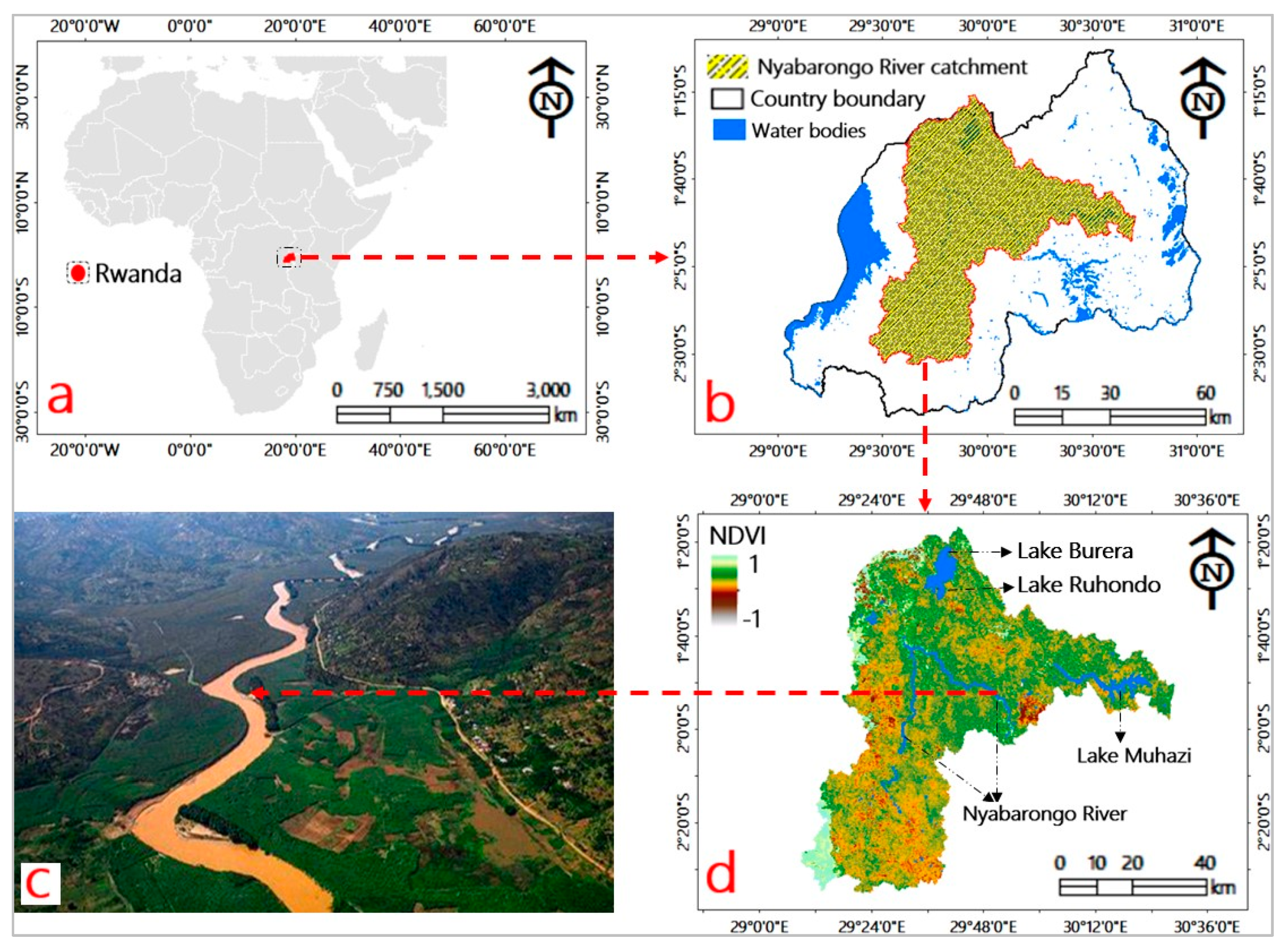
Rwanda is a country endowed with abundant water resources distributed in a very dense hydrological network consisting of lakes, marshlands, and rivers [45]. The country is made of two hydrographical basins defined by a landmark line of waters known as the Congo–Nile divide that runs from the north to the south. To the east of the Congo–Nile divide lies the Nile basin with two main river catchments, namely, the Akagera and the Nyabarongo. The latter is located between 1°18′ S to 2°34′ S latitude and 29°5′ E to 30°35′ E longitude with an approximated length of 151.5 km, draining a total area of 8478.24 km² [43]. The Nyabarongo catchment (Figure 1) goes along a path up to the north-western region of the country, then crosses the center to the south-east, to form the focal tributary of the Kagera River, flowing into Lake Victoria. It also flows easterly via small lakes and swampy valleys in the plains of Bugesera-Gisaka. Moreover, it flows over 300 km from its source in the West into Lake Rweru (the outlet of the catchment) in South Eastern Rwanda, lateral to the border with Burundi [46,47]. As the largest river catchment in the entire country, it covers different districts from all the provinces countrywide, including the highly urbanized region of Kigali city [48]. Topographically, the catchment’s elevation ranges between 1332 m to 4480 m above sea level [43]. Like the rest of the country, this relief profile contributes to the variation in weather patterns [49,50]. The area enjoys tropical climatic conditions, with two rainy seasons each year. The first season is known as the long rainy season (March to May), and the second the short rainy season (September to November)—both periods in which heavy rainfall-induced hazards are expected.

2.2. Data Collection and Processing

Hydro-meteorological (rainfall and flow) along with physiographic data (digital elevation model, land use/cover, and soil type) are significant inputs in rainfall-discharged flow modeling (

Table 1. The spatial databases for datasets included in this data.

Data Type	Spatial Resolution	Source
Digital Elevation Model (DEM)	1 arc-second (~30 m, raster data)	Earth Explorer (USGS)
LULC map	30 m × 30 m (raster data)	Landsat 8 OLI (USGS)
Soil properties map	30 arc-second (raster data)	FAO-UNESCO Soil Map of the World
Rainfall data	Daily rainfall (2011–2018)	Rwandan Meteorological Agency (RMA)
Flow data	Daily flow (2011–2018)	Rwandan Meteorological Agency (RMA) and Rwanda Water Portal

). Rainfall characteristics were considered as representative of the supply of water to the catchment—a portion of which reaches the outlet as discharge. Generally, hydrologic models often require time-series of precipitation and observed flow, which help in model calibration and validation [52]. However, the topographical features of the country hindered and limited the installation and maintenance of sufficient rain gauge networks required for capturing the variability in rainfall over the space. Moreover, weather radars, as an alternative for precipitation data capturing, are not a viable choice for this study area owing to the presence of radar beam blockage resulting from the surrounding mountains. Thus, this study considered the available hydrological data (daily rainfall and observed flow) from 2011 to 2018 recorded at the Rweru gauging station (the outlet of the study area) and collected from the Rwandan Water Portal and the Rwandan Meteorological Agency (RMA). This period was selected due to the availability of both rainfall and flow data with no gaps. These data are from the rainfall seasons from March to May (long rainy) and September to November (short rainy).

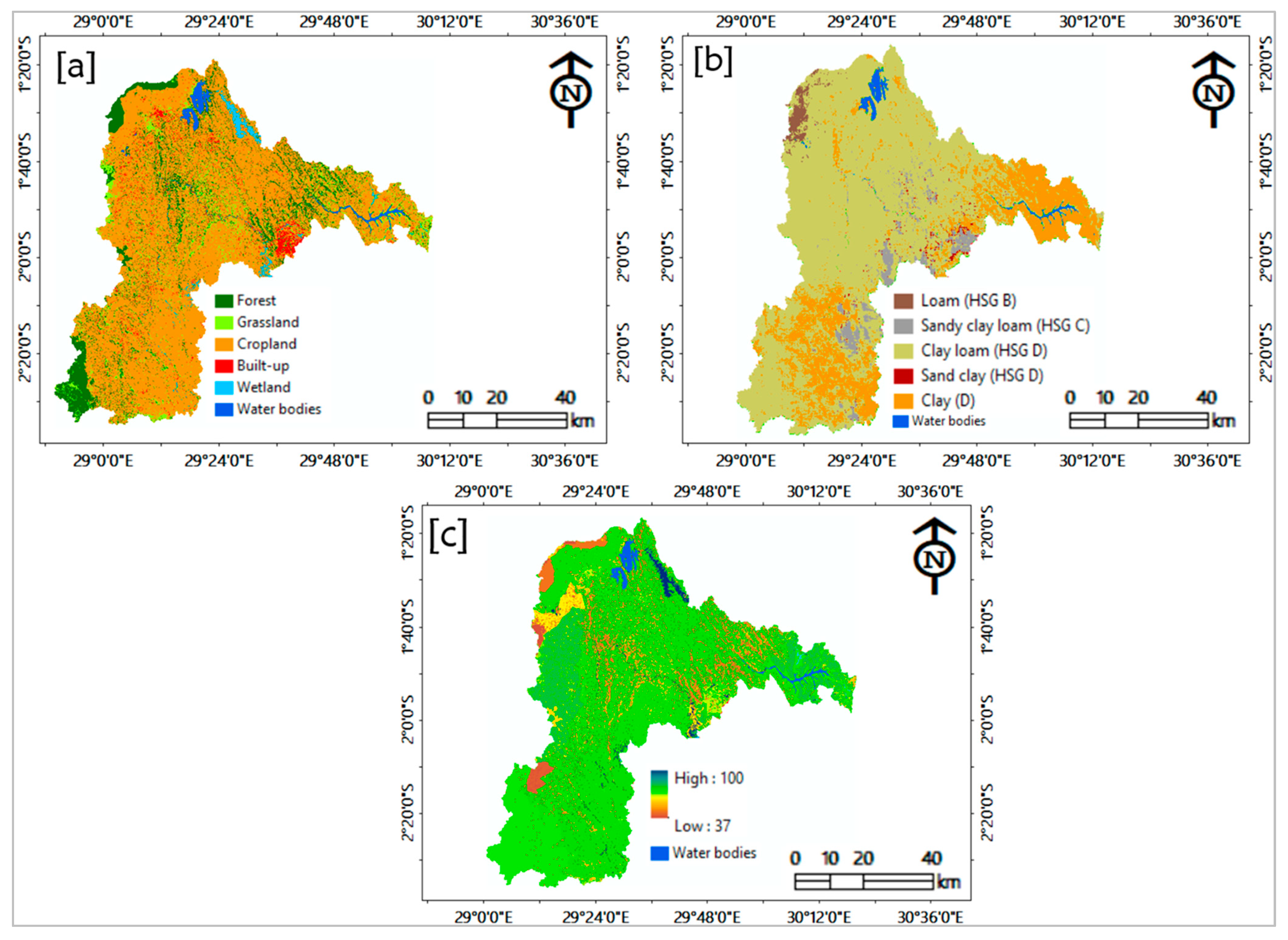
Besides this, a 30 m resolution (1 arc-second) digital elevation model (DEM) from the Shuttle Radar Topographic Mission (SRTM) provided by the National Aeronautics and Space Administration (NASA; www.dwtkns.com/srtm30m/ accessed on 17 May 2021) was used to extract the topographic characteristics of the study area. Additionally, land use/cover (LULC) and soil properties (Figure 2a,b) play an imperative role in catchment hydrology [53]. The latter were applied in order to model accurate hydrologic processes. The LULC was obtained by processing Landsat-8 imagery with low cloud cover assembled by the United States Geological Survey (USGS) and classified using the maximum likelihood classification (MLC) technique in ENVI software version 5.3. Atmospheric and radiometric corrections were executed with the Fast Line-of-Sight Atmospheric Analysis of Hypercube (FLAASH) tool to lessen atmospheric effects and radiometric errors, in order to increase the interpretability and quality of the image before the classification procedure. The data on soil properties were extracted from a raster file of the global soil type using ArcGIS 10.8. The soil properties map was fully prepared in detail using information from the World Harmonized Soil Database (HWSD) viewer, downloaded at http://www.fao.org/soils-portal/data-hub/soil-maps-and-databases/harmonized-world-soil-database-v12/en/ (accessed on 9 February 2021).

2.3. HEC-HMS Model Description and Catchment Delineation

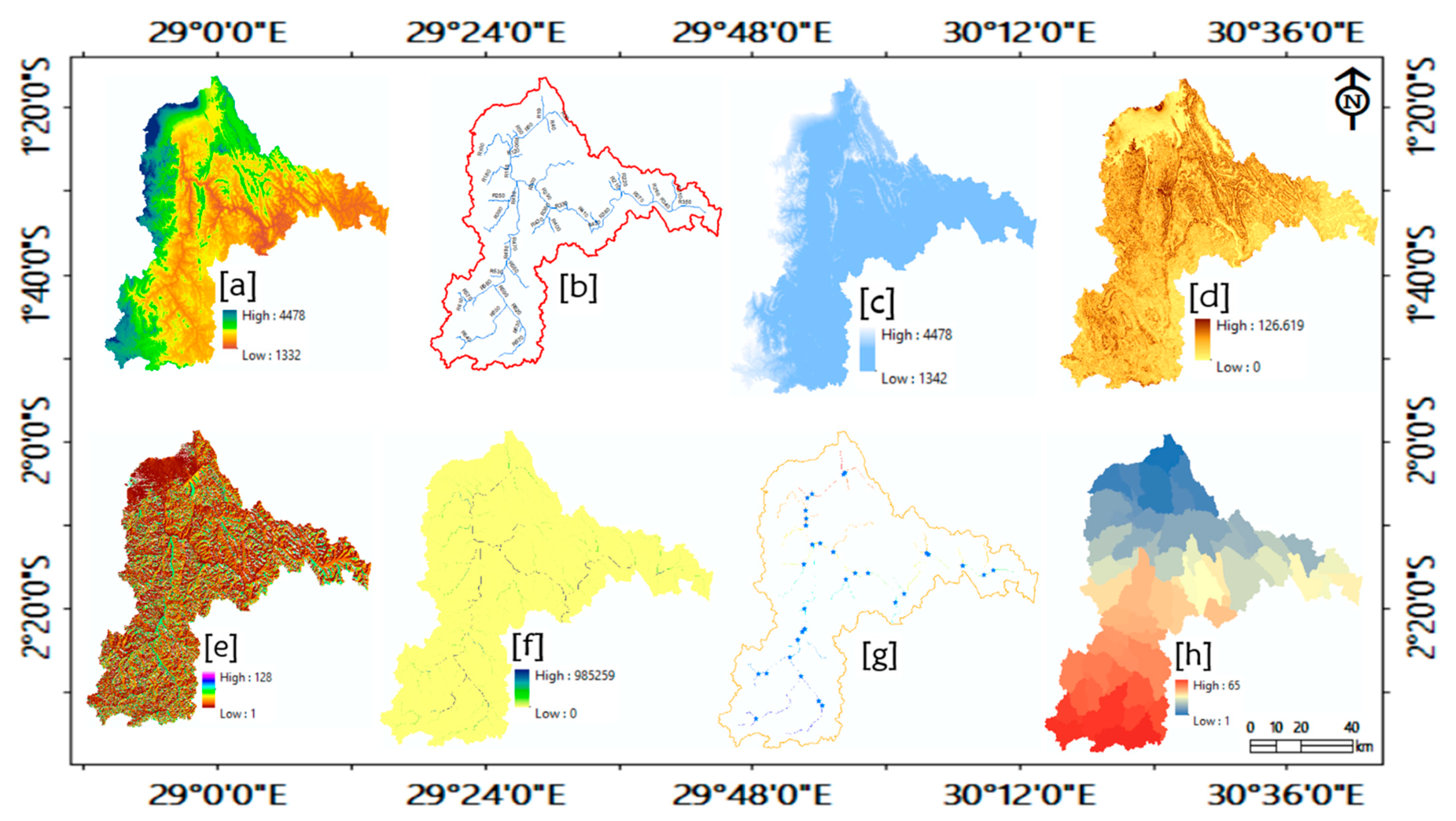
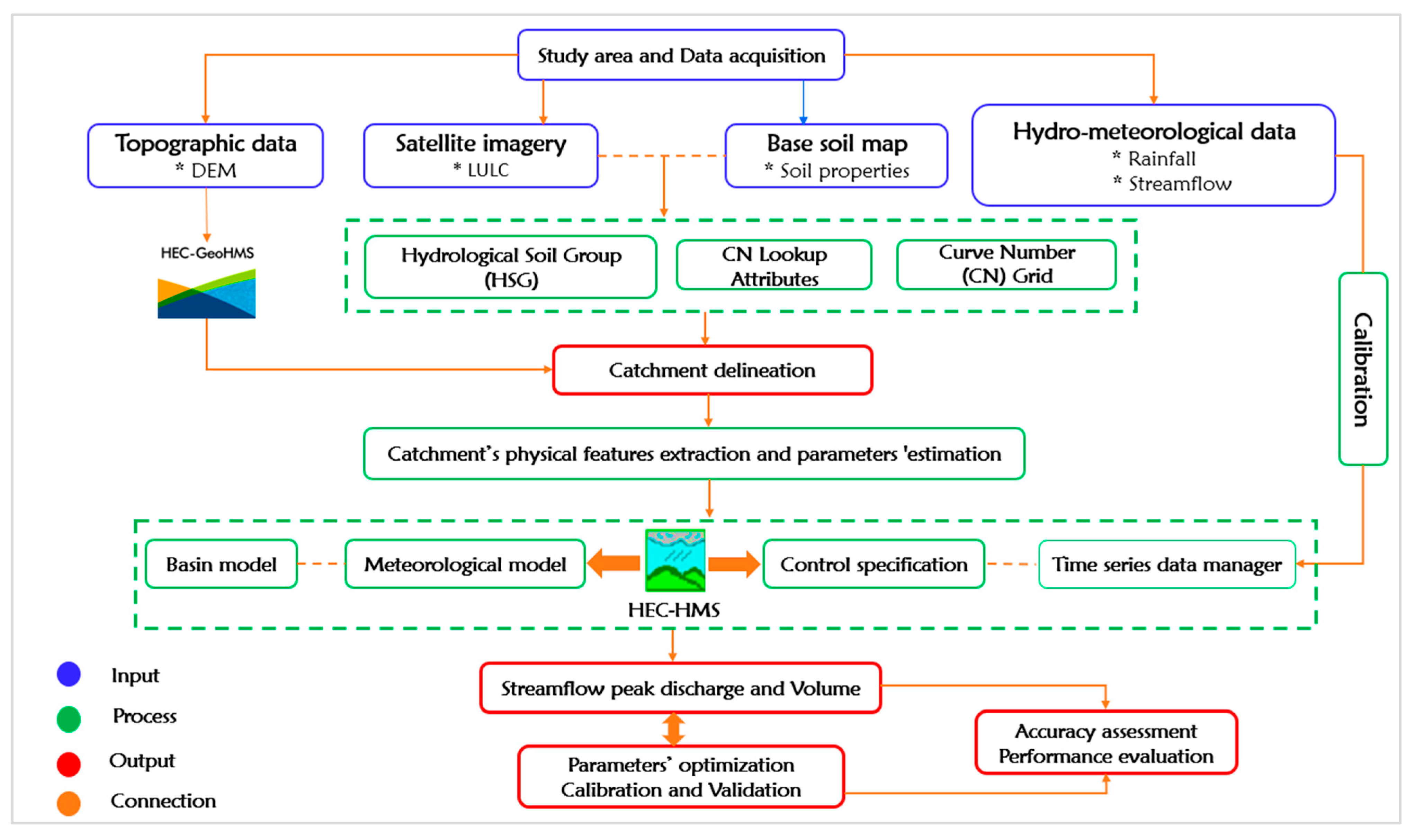
HEC-HMS software was established by the United States (US) Army Corps of Engineers (http://www.hec.usace.army.mil/software/hec-hms accessed on 3 February 2021). This study utilized the current version 4.7.1 to simulate rainfall-discharged flow processes. Initially, the collated DEM was exploited and pre-processed using the Arc Hydro tool, then applied the Hydrologic Engineering Center-Geospatial Hydrologic Modeling (HEC-GeoHMS), a geospatial tool extended in ArcGIS 10.8 to generate spatial data relating to the stream network and terrain features (Figure 3). Moreover, the tool helped to produce the required parameters which could be used as input data for the HEC-HMS setup [28]. In the catchment delineation process and subbasins hydrological parameters, a threshold of 75 km² drainage area was given for stream definition and physiographic characteristics, including the basin slope and centroid, river length, and longest flow path, among others. The LULC and soil properties were then combined to assign curve numbers (CN) using the generated CN lookup attributes (Table S1); each LULC category was classified, according to the resulting hydrological soil classes based on the texture classes (Figure 2a–c). After all the above steps, the catchment boundaries and drainage paths were transformed into a structured hydrologic database that denoted the catchment response to rainfall using HEC-GeoHMS [54]. The HEC-HMS setup comprised four imperative components: namely, the basin model, meteorological model, control specifications, and time-series data manager [55]. The basin model consisted of the delineated hydrologic elements (subbasin, junction, reach, source, sink, reservoir, diversion, outlet) and their connectivity, characterizing the flow of water to the drainage system, while the meteorological model detailed the elements over which precipitation input is temporally and spatially distributed throughout the catchment. Additionally, the control specification denotes the time of simulation, and finally, the time series data manager dealt with input data [56]. The model ran by combining the information populated in these four units to attain the results.

2.4. Parameter Estimation in HEC-HMS and Methods

HEC-HMS produces results using different algorithms that represent each element of the flow process, including those that compute the volume and direct runoff [9,28]. These algorithms are based on input value parameters such as the losses, transform, and routing of meteorological data. The selection of these methods is based on their suitability and limitations, accessibility of data, hydrologic conditions, researcher recommendations, etc.

2.4.1. The Loss Method

This method is applied to estimate the excess runoff volume by calculating the water which has been intercepted, infiltrated, stored, evaporated, and withdrawn from rainfall. Various approaches have been applied to model and produce values for this parameter, but the Soil Conservation Service (SCS) curve number (CN) approach has been applied in this study due to its simplicity in estimating the volume from a rainfall event and the fact that it is reinforced by empirical data. This method is a function of LULC and soil properties as the major runoff-producing catchment characteristics from an amount of rainfall. The SCS-CN approach established by the Soil Conservation Service [57,58] was computed using the following equation:

$$\mathrm{Q}=\frac{{\left(\mathrm{P}-{\mathrm{I}}_{\mathrm{a}}\right)}^2}{\mathrm{P}-{\mathrm{I}}_{\mathrm{a}}+\mathrm{S}}$$

(1)

where Q is the direct runoff (volume in mm for the total event), P is the cumulative rainfall for the event in mm, I_a for the initial abstraction, and the potential maximum retention (S).

However, the loss method allows the choosing of the process used to calculate the rainfall losses (I_a) absorbed by the ground, calculated as 20% of the total maximum retention (S) of the catchment. It also requires the soil curve number (SCS curve number) for each delineated sub-basin. I_a and S are computed using Equations (2) and (3), respectively.

$${\mathrm{I}}_{\mathrm{a}}=0.2\mathrm{S}$$

(2)

$$\mathrm{S}=25.4\left(\frac{1000}{\mathrm{CN}}-10\right)$$

(3)

2.4.2. Transform Method

The transform method is used to simulate the process of direct runoff and excess rainfall on the catchment as well as transform rainfall excess into point runoff via a unit hydrograph. For this process, this study used the SCS unit hydrograph approach, whereby the standard lag time (T_Lag) is entered as an input parameter to evaluate the time between rainfall and peak flow in the catchment; it is estimated using Equation (4), as proposed by USDA [59]:

$${\mathrm{T}}_{\mathrm{Lag}}=\frac{{\mathrm{L}}^{0.8}{\left(\mathrm{S}+1\right)}^{0.7}}{1900\times {\mathrm{Y}}^{0.5}}$$

(4)

where T_Lag is the lag time in hours, S is the maximum retention, L is the hydraulic length of the catchment, and Y is the slope of the sub-basin.

2.4.3. Routing Method

Routing methods simulate the attenuation of flood runoff when traveling through the reach due to channel storage effects [9]. Numerous techniques for this simulation are applied to flood routing in gauged basins, due to their requirement of large amounts of observed data. Owing to the scarcity of extensive observed data, this study applied the routing technique proposed by Song, Kong [60], built based on the Muskingum model, with parameters derived from the physical characteristics of the river reach. This technique has been satisfactory and proved to remove the difficulties in predicting flow characteristics in poorly gauged and ungauged catchments. Its advantage lies in its simplicity and its being the only diffusion-wave routing model which is accurate enough to be suitable for hydrologic modeling applications [61]. This method necessitates the routing parameters K and X [54], estimated using the geometric shape and characteristics of the channel cross-section, which simulate the relative involvement of hydrodynamic and kinematic diffusion. K represents the storage-time constant, while X is a weighted factor usually ranging between 0 and 0.5. These were then computed using the following Equations (5) and (6), respectively:

$$\mathrm{K}=\frac{0.69{\mathrm{n}}^{0.6}{\mathrm{LC}}^{0.4}}{3600{\mathrm{Q}}_0^{0.2}{\mathrm{S}}^{0.3}}$$

(5)

$$\mathrm{X}=\frac{1}{2}-\frac{0.35{\mathrm{Q}}_0^{0.3}{\mathrm{n}}^{0.6}}{{\mathrm{S}}^{1.3}{\mathrm{C}}^{0.8}\mathrm{L}}$$

(6)

where n denotes the manning roughness coefficient that represents the resistance to water flows in the channels. Its values are tabulated and represented in the literature from different reference books and articles based on expert experiences and knowledge of different distinctive river channels in terms of physical features [62,63,64,65]. Hence, n was set to 0.035 for the Nyabarongo River catchment, described as an open natural channel flow composed by major rivers, some types of vegetation, and dominated by farmlands. L represents the hydraulic length of the river reach (m), C specifies a coefficient defining celerity, S is the slope, and Q₀ is the reference flow (m³·s⁻¹) for a given reference flow event computed according to Wilson and Ruffini [66], using Equation (7):

$${\mathrm{Q}}_0={\mathrm{Q}}_{\mathrm{i}}+\frac{1}{2}\left({\mathrm{Q}}_{\mathrm{j}}-{\mathrm{Q}}_{\mathrm{i}}\right)$$

(7)

where Q_i and Q_j represent the minimum and peak flow, respectively. Note that a stand-alone GIS-based terrain analysis program supported the estimation of all the above variables in the determination of routing parameters.

2.5. Calibration and Validation

Before a hydrological model can be considered as having reliable outputs, it needs to be calibrated and validated through an observed flow (Figure 4). The simulated and observed flow should be compared to test how well they fit and deduce the credibility of results produced by the model. The accessible hydrometeorological data is divided into two parts for calibrating and validating the model; in this study, 16 rainfall events (

Table 2. Rainfall events selected for calibration and validation.

Events	Start Date	Start Time	End Date	Start Time	Remark
1	LR: 21 Mar 2011	00:00	18 May 2011	00:00	calibration
2	SR: 06 Sep 2011	00:00	15 Nov 2011	00:00	calibration
3	LR: 10 Mar 2012	00:00	27 May 2012	00:00	calibration
4	SR: 13 Sep 2012	00:00	19 Nov 2012	00:00	calibration
5	LR: 15 Mar 2013	00:00	12 May 2013	00:00	calibration
6	SR: 09 Sep 2013	00:00	13 Nov 2013	00:00	calibration
7	LR: 11 Mar 2014	00:00	14 May 2014	00:00	calibration
8	SR: 12 Sep 2014	00:00	15 Nov 2014	00:00	calibration
9	LR: 20 Mar 2015	00:00	18 May 2015	00:00	calibration
10	SR: 23 Sep 2015	00:00	22 Nov 2015	00:00	calibration
11	LR: 24 Mar 2016	00:00	22 May 2016	00:00	Validation
12	SR: 12 Sep 2016	00:00	15 Nov 2016	00:00	Validation
13	LR: 12 Mar 2017	00:00	14 May 2017	00:00	Validation
14	SR: 18 Sep 2017	00:00	23 Nov 2017	00:00	Validation
15	LR: 10 Mar 2018	00:00	12 May 2018	00:00	Validation
16	SR: 13 Sep 2018	00:00	15 Nov 2018	00:00	Validation

LR: Long rainy and SR: Short rainy.

) recorded in the period from 2011–2018 were selected and split into 2 categories, such that 60% (2011–2015) were used for calibration and the remaining 40% were used for validation (2016 to 2018).

The comparison of the observed against the simulated flow was done at the outlet (computation point) where the observed flow gauging station was available. It should be noted that there are always uncertainties in the modeled parameter values. Therefore, some adjustments of the parameters are often required to closely fit the observed and simulated discharged flow. For this task, the automatic optimization process embedded within HEC-HMS was exploited using the univariate gradient optimization package and the peak-weighted root mean square error (PWRMS) objective function to move from the initial parameter to the final best parameter estimates [28]. Thus, the degree of variation between simulated and observed hydrographs was quantified. The latter was helpful in the sensitivity analysis for identifying the parameters which had most influence on the model performance for the study area.

2.6. Performance Evaluation

As the most common metrics used to forecast the accuracy of the model for the selected loss and transform methods, the Nash Sutcliffe Efficiency (NSE; Equation (8)), the correlation coefficient (R²; Equation (9)), and the relative errors (RE; Equation (10)) of the peak flow and volume (RE_F,V) were computed to indicate the accuracy between observed and simulated values:

$$\mathrm{NSE}=1-\frac{{{\displaystyle \sum }}_{\mathrm{j}=1}^{\mathrm{n}}{\left({\mathrm{X}}_{\mathrm{j}}-{\mathrm{Y}}_{\mathrm{j}}\right)}^2}{{{\displaystyle \sum }}_{\mathrm{j}=1}^{\mathrm{n}}{\left({\mathrm{X}}_{\mathrm{j}}-\overline{\mathrm{X}}\right)}^2}$$

(8)

$${\mathrm{R}}^2=\frac{{\left[{{\displaystyle \sum }}_{\mathrm{j}=1}^{\mathrm{n}}\left({\mathrm{X}}_{\mathrm{j}}-\overline{\mathrm{X}}\right)\left({\mathrm{Y}}_{\mathrm{j}}-\overline{\mathrm{Y}}\right)\right]}^2}{{{\displaystyle \sum }}_{\mathrm{j}=1}^{\mathrm{n}}{\left({\mathrm{X}}_{\mathrm{j}}-\overline{\mathrm{X}}\right)}^2{{\displaystyle \sum }}_{\mathrm{j}=1}^{\mathrm{n}}{\left({\mathrm{Y}}_{\mathrm{j}}-\overline{\mathrm{Y}}\right)}^2}$$

(9)

$${\mathrm{RE}}_{\mathrm{F},\mathrm{V}}=\frac{\left|{\mathrm{Y}}_{\mathrm{j}}-{\mathrm{X}}_{\mathrm{j}}\right|}{{\mathrm{X}}_{\mathrm{j}}}\ast 100$$

(10)

where n is the flow duration in Equation (8), and the number of errors in Equation (9); Y_j is the simulated data value at time j; X_j is the observation data value at time j; while $\overline{x}$ and $\overline{y}$ are the average of observation and simulated values, respectively.

3. Results and Discussion

3.1. Physiographical Attributes of the Delineated Catchment

In HEC-HMS, the catchment is conceptually represented as a mesh of sub-areas interconnected by channel links [67]. For the hydrologic modeling project, the obtained results from the pre-processed topographic terrain using the geospatial hydrologic analysis module are tabulated in

Table 3. Physiographic characteristics of the delineated Nyabarongo catchment.

No	SB	Area (Km2)	Slope	Mean River Slope	Hydraulic Length (m)	Main River Length (m)
1	W1230	863.61	2084.79	−0.013902	41,001.49	12,868.13
2	W1140	1139.6	1758.01	0.004494	88,558.16	37,835.82
3	W960 **	710.51	1626.83	0.015872	48,008.99	25,294.14
4	W1290	951.6	1809.49	0.012851	59,373.68	36,844.79
5	W900	772.62	2146.6	0.022433	56,614.21	27,817.45
6	W720	1239.9	2165.07	0.027237	62,084.87	31,250.99
7	W870	1186.8	1651.9	0.00835	72,337.23	22,147.99
8	W690	1613.6	1846.41	0.013222	71,698.25	31,959.94
9	R440 **	736.9	0.002714	-	-	-

**: means subbasin or reach at the outlet.

.

Note that negative numerals do not specify minus as in algebraic expressions, but simply differentiate the up and downhill slopes. The parameter estimates representing the loss and transform model per each sub-basin are tabulated in Table S2.

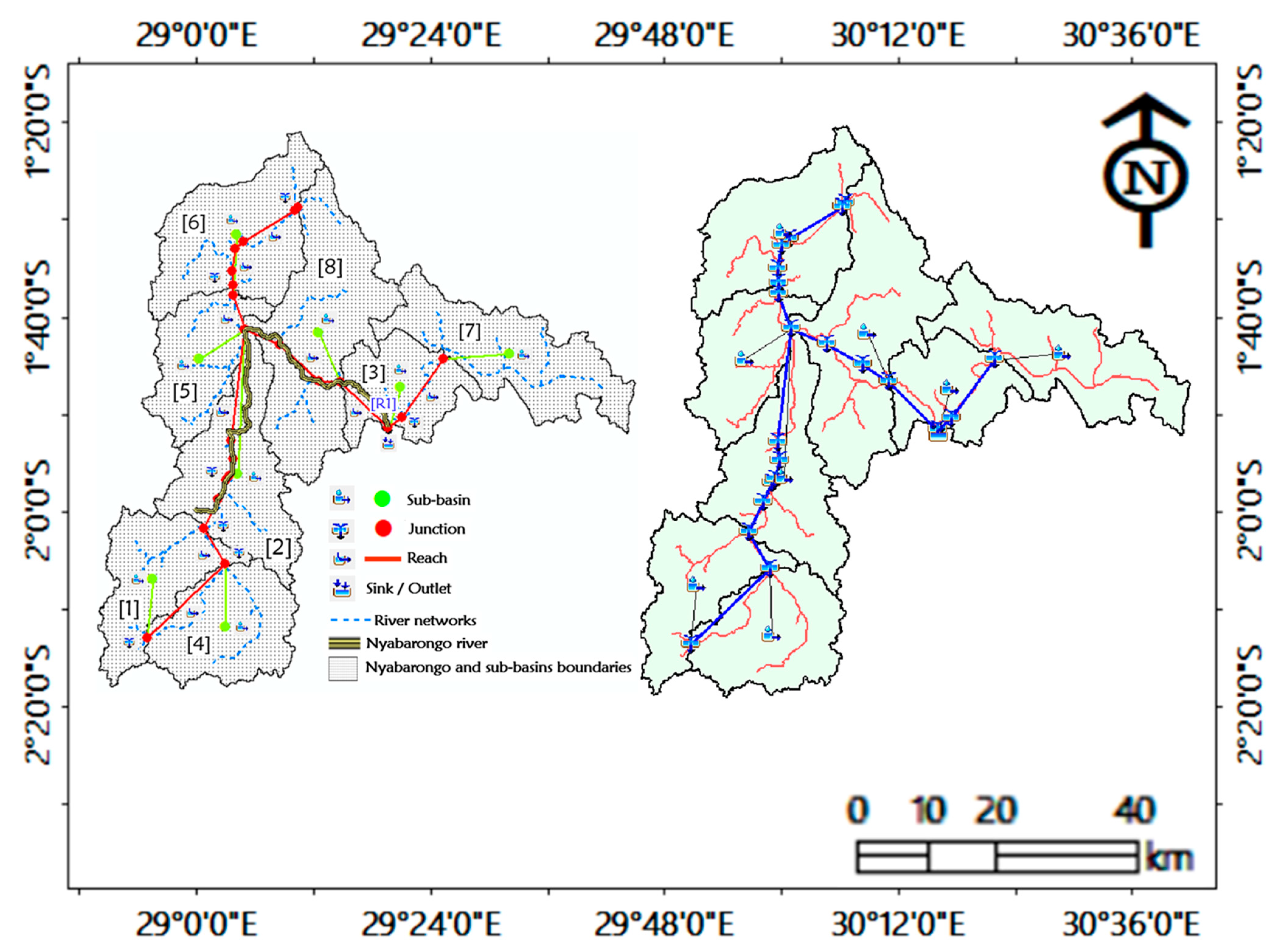
As demonstrated in the resulting schematic catchment model (Figure 5) with all the hydrologic elements, the delineated Nyabarongo catchment was subdivided into eight sub-basins, twenty-three reaches, their related junctions, and one outlet, depending on the set critical area threshold for stream generation. All other generated initial values per reach can be found in Table S3. As in this study, the considered reach (R440) was the one related to the outlet where the calibration took place. Each subbasin was shown to be connected to the upstream node of its downstream reach, which is a junction defined by the reach coordinates (Figure 5). The sub-basin areas ranged from 710.51 sq.km to 1613.6 sq.km, while the length of the main rivers ranged from 4.7 to 44.8 km. Analogous with the classified LULC of the area (Figure 2a), the third sub-basin (W960) containing the catchment’s outlet, was the most urbanized. In line with this finding, previous studies [68,69] reported that urbanizing catchments greatly impact the hydrologic process in terms of flood peak advancement and increases in surface runoff. The associated presence of prevalent impervious surfaces alters the dynamics of infiltration by reducing the quantity of water that can immerse into the ground [70,71]. Additionally, cropland was the dominant land use class through the entire catchment. This result also gives a reflection on the amount of runoff that can produce the catchment, in conjunction with previous studies [72,73,74] reporting that the runoff becomes excessive to various degrees in cropland, urban landscapes, and bare surfaces. Thus, this result implicates the probability of high surface runoff generation leading to flooding in this area.

3.2. Hydrological Response of the Catchment under Rainfall Events

The generated physiographic parameters and their values, along with the hydro-meteorological data, were introduced into the HEC-HMS model to simulate peak flow and volume through calibration and validation, and therefore, determine the hydrological response of the catchment.

3.2.1. Calibration and Optimization

After appropriate calibration for each selected loss, transform method, and routing reach, the hydrological response of the catchment was measured through the simulated peak flow and volume, as they went in parallel with maximum downstream flooding based on rainfall events [75,76]. The obtained model outputs (peak flow/volume) were reasonable in comparison to the observed data at the gauging station, although for some events, the model largely over or underestimated the peaks prior to optimization (

Table 4. Observed and simulated peak flow/volume before and after optimization.

Selected Events		Peak Flow (cms)			Volume (mm)			Accuracy Assessment
Events	Start and End Date	SBO	SAO	Obs	SBO	SAO	Obs	REF (%)	REV (%)	R2	NSE
1	LR: 21 Mar–18 May 2011	98.5	100.8	109.8	103.83	105.77	117.55	8.9	11.14	84.7	81.8
2	SR: 06 Sep–15 Nov 2011	97.8	86.4	89.4	115.58	127.92	140.94	3.4	10.2	88.8	81.6
3	LR: 10 Mar–27 May 2012	136.8	132.4	123.0	144.83	162.32	182.22	7.0	6.4	92.6	89.4
4	SR: 13 Sep–19 Nov 2012	112.2	97.9	95.2	122.7	131.82	139.0	2.8	5.4	86.8	74.3
5	LR: 15 Mar–12 May 2013	166.9	166.9	174.5	140.04	148.59	156.98	4.5	5.6	94.5	93.5
6	SR: 09 Sep–13 Nov 2013	90.2	83.4	82.1	145.52	144.61	156.08	1.6	7.9	81.8	74.2
7	LR: 11 Mar–14 May 2014	133.4	134.6	126.9	146.73	169.19	173.68	5.7	2.6	89.7	80.2
8	SR: 12 Sep–15 Nov 2014	88.4	85.3	82.1	107.13	110.4	122.63	3.7	11.0	86.6	81.8
9	LR: 20 Mar–18 May2015	169.7	171.7	192.5	200.52	204.73	218.53	12.1	6.7	90.6	82.8
10	SR: 23 Sep–22 Nov 2015	148.0	132.7	125.8	120.87	133.86	147.97	5.2	10.5	87.7	74.4
Mean								5.5	7.7	88.4	81.4

Where cms: cubic meter per second; SBO: simulation before optimization; SAO: simulation after optimization; Obs: observation.

). This situation can evoke the over-reach of mitigation initiatives or unsatisfactory planning for probable situations unless there is a careful sensitivity analysis [77,78]. To obtain this condition, an optimization session was conducted to bring the simulated and observed flow/volume closer. After optimization, the model simulated the values reasonably close to the observed flow values for the overall simulation events. However, the model could not fully generate values that exactly fit the observed and simulated data, due to some uncertainties arising from either the edifice of the model concept itself, or the variables, observed inputs, or interconnection processes. The urbanizing situation at the outlet may also create uncertainties if the surface model does not fully consider the intricate infrastructure of the urbanized location.

Except events 1, 5 and 9 during the calibration process, the simulation results have shown a tendency to overestimate the peak before optimization, while 40% of the events (events 1, 2, 5, 9) have underestimated the peak flow after optimization. Besides this, an underestimation of the volumes was depicted for all the events prior to optimization, while none of the events were shown to overestimate the volume after optimization. Similar to this study, Hussain, Wu [28] and Arheimer and Lindström [79] argued that the underestimation of high peak flows during the rainy season can be attributed to unregulated observation data or slight increases in flow at the beginning of the season, owing to the early arrival of the rain. Overall, it was noted that the optimization step played a pivotal role for events which largely over or underestimated the flow and volume compared to the observed values. From these obtained results, it is clear that the amount of flow depends on the received rainfall. Thus, it can be said that the existing hydrological response of the Nyabarongo River catchment is directly associated with the rainfall seasons of Rwanda; a result which is in agreement with Kibria, Ahiablame [80] and Khalil, Rittima [81], where the trend magnitude for seasonal streamflow increased in fall and wet seasons compared to other seasons. Such results suggest that the catchment’s hydrology is vulnerable to any change in climate as well as its related rainfall patterns over a period of time, as also confirmed by previous studies [82,83,84]. This trend is almost the same over the entire hydrological system of Rwanda, characterized by high peak flows mainly during the periods of March to May (long rainy) and moderate flows during September to November (short rainy). Note that in the remaining periods, such as June to August (long dry) and November to February (short dry), which were not considered in this study, only low flows are expected. The high and moderate flows are among the main factors contributing to flooding incidences in districts in which the Nyabarongo River runs, including Kamonyi, Kicukiro, Nyarugenge, Kamonyi, Muhanga, Gakenke, Ruhango, and Rulindo, among others [49,85].

3.2.2. Sensitivity Analysis of Parameters

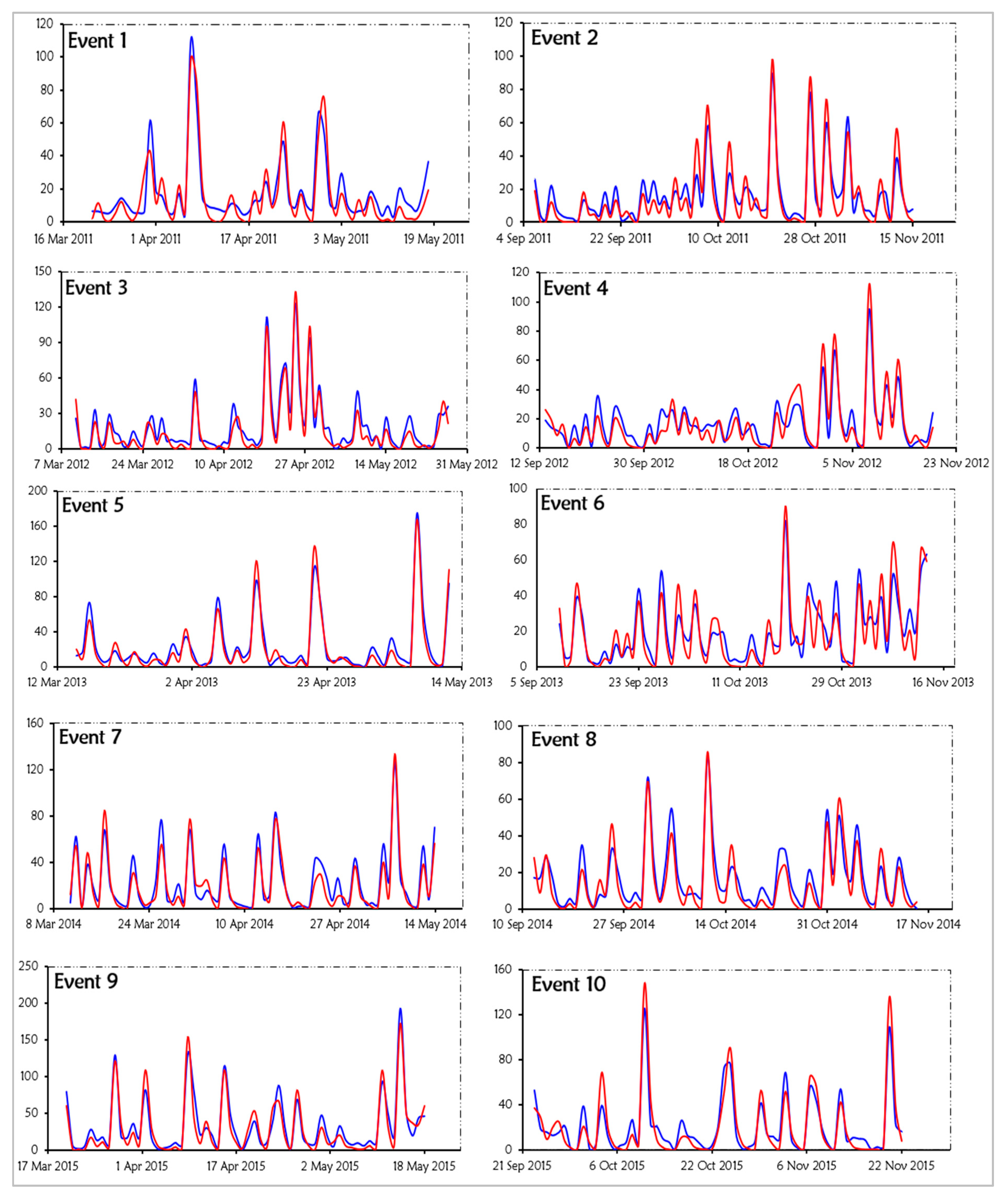
Generally, the development of acceptable flow simulations in a catchment does not necessarily result in accurate performances of runoff production processes [77]—this is because diverse parameters in the comprehensive catchment model are reported to be sensitive; and thus, influence the calibration processes of the model. The analysis determined the parameters whose modification significantly affected the outputs of the model. The parameter values required for calibration were calculated and given as initial values at the time of calibration to the selected model. The modeled hydrograph results (Figure 6) that managed to capture the observed hydrograph with a good fit were maintained while poor results proceeded to the optimization stage. As reported by Belayneh, Sintayehu [86], and Zheng, Li [87], the initial abstraction and its related maximum retention, curve number (CN), lag time, and Muskingum parameters were the most significantly sensitive parameters in the model. In this study, the parameters showed some dynamicity in their values compared to the initial values, except for lag time, which remained insensitive to the calibrated events and was not influenced by differences in rainfall (

Table 5. Initial and optimized values for the parameters in the sensitivity analysis.

Selected Events		Ia		S		CN		TLag		K		X
Events	Period	IV	OV	IV	OV	IV	OV	IV	OV	IV	OV	IV	OV
1	LR	10	14.9	50.03	74.5	83.516	78.2	68.4	68.4	0.08	0.05	0.34	0.48
2	SR		8.5		42.5		89.8		68.4		1.98		0.21
3	LR		12.9		64.5		82.9		68.4		1.67		0.41
4	SR		14.4		72		78.2		68.4		2.2		0.43
5	LR		7.9		39.5		80		68.4		0.13		0.37
6	SR		14.5		72.5		59.6		68.4		0.34		0.49
7	LR		13.7		68.5		88.9		68.4		3.48		0.39
8	SR		15.1		75.5		91.6		68.4		0.03		0.28
9	LR		7.2		36		75		68.4		2.59		0.31
10	SR		8.9		44.5		42.2		68.4		1.78		0.4
Mean	-		12.4		62		80.66		68.4		1.43		0.38

IV: Initial values, OV: Optimized values.

), as similarly evidenced by Hamdan, Almuktar [54]—who recently found simulated flow to be less affected by the delay between the maximum rainfall amount and the peak discharge in the Al-Adhaim River catchment covered by agricultural land. The Muskingum parameters have been shown to be the most sensitive, with a high influence on the simulated peak flow and volume values. This conformed with a previous study [88] which modeled the rainfall–runoff relationship in the upper Awash catchment, Ethiopia. The latter was followed by the initial abstraction and its related maximum retention—the reason being that rainfall characteristics normally play a noteworthy role in the ascertainment of abstraction duration, and thus, in the calculation of flow hydrographs. This has also been reported by previous studies, not only for small catchments [77,89], but also for large-scale catchments [90]. Finally, changes in CN values often show a dynamic and quantitative impact on simulated discharged flow and volume. Therefore, selecting an appropriate CN value is necessary for generating consistent outputs in hydrological modeling, owing to its reported sensitivity to the simulated flow and volume. In this study, the CN parameter was also found to be more sensitive to rainfall excess, percolation, and permeability mechanisms compared to the hydrological soil groups (Figure 2b), as similarly discussed by preceding studies [91,92]. From the same perspective, a recent study specified that a given amount of rainfall may generate completely different discharged flow and runoff volumes under different assigned CN during hydrological modeling phases [93]. Nevertheless, the sensitivity analysis in this study justifies the necessity of acquiring appropriate land surface characteristics such as the LULC and soil information, in order to attain a more precise estimation of the CN of the study area.

3.2.3. Validation

Model validation runs the model using similar inputs and calibrated parameter estimates. After optimization of the parameters, some events displayed values that decreased as the agreement between observed and simulated values increased, and others increased as goodness-of-fit increased. In this validation process, the model results exposed a slight overestimation of the peak flow and underestimation of the volumes for all the events except event 13, which had estimated values closer to acceptable levels (

Table 6. Observed and simulated peak flow and volume for validation process.

Selected Events		Peak Flow (cms)		Volume (mm)		Accuracy Assessment (%)
Events	Start and End Date	Simulated	Observed	Simulated	Observed	REF	REV	R2	NSE
11	LR: 24 Mar–22 May 2016	152.1	148.1	141.48	156.84	2.6	10.8	88.3	81.8
12	SR: 12 Sep–15 Nov 2016	94.8	88.9	100.46	105.37	6.2	4.8	90.5	86.1
13	LR: 12 Mar–14 May 2017	169.9	172.7	245.9	242.56	1.6	1.3	94.4	91.5
14	SR: 18 Sep–23 Nov 2017	94.4	88.1	131.85	140.89	6.7	6.8	87.9	81.5
15	LR: 10 Mar–12 May 2018	177.7	174.8	265.98	266.85	1.6	0.3	92.2	91.2
16	SR: 13 Sep–15 Nov 2018	87.3	83.4	107.28	111.46	4.5	3.8	85.9	75.8
Mean						3.8	4.6	89.8	84.6

). This latter finding has also been detected by earlier hydrological modeling studies [9,94], with such findings addressing the uncertainty involved in model simulations. Nonetheless, the significance of this type of study is not to portray an exact value, but rather, to provide an estimation for a comprehensive understanding of probable future scenarios for researchers and policymakers.

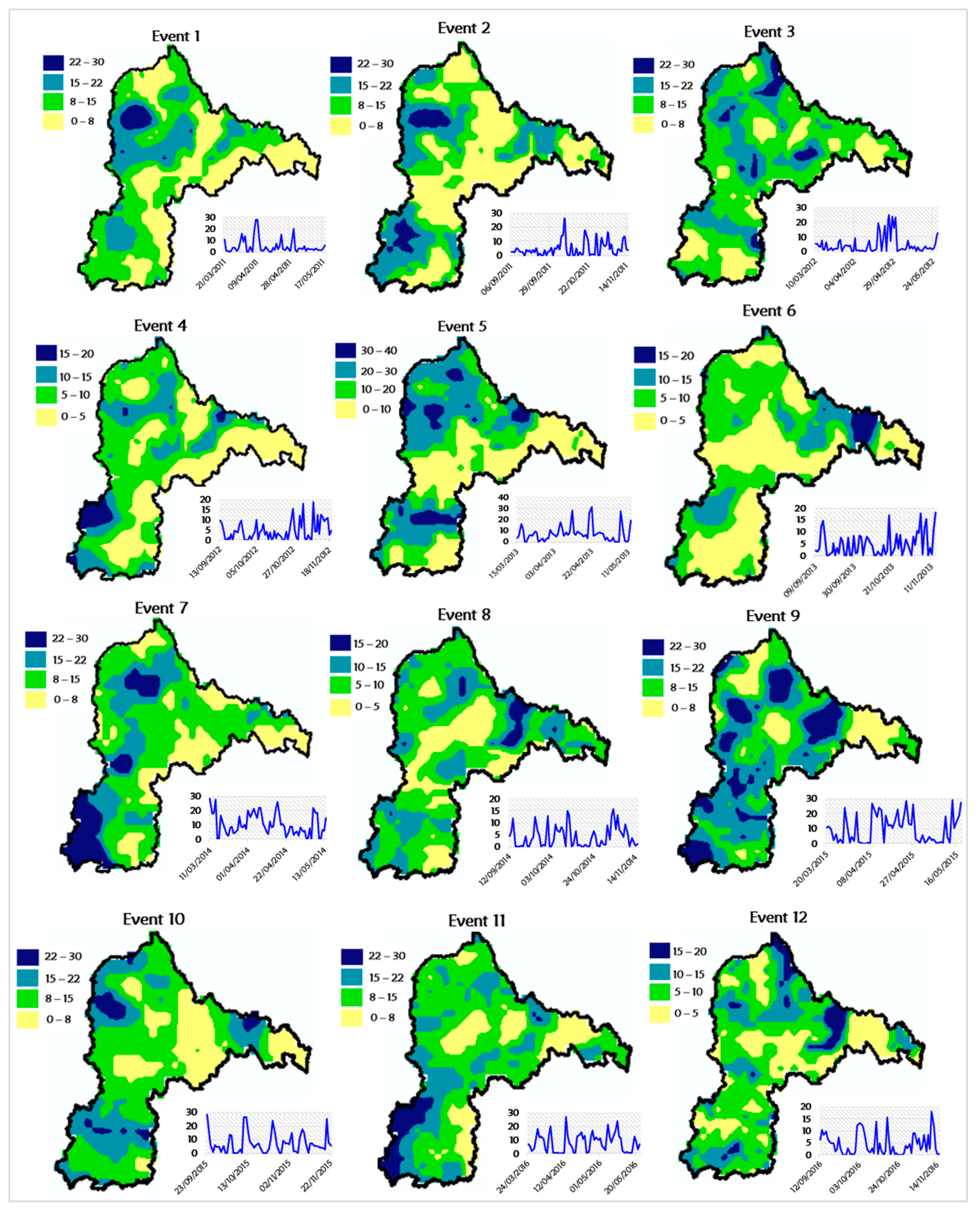
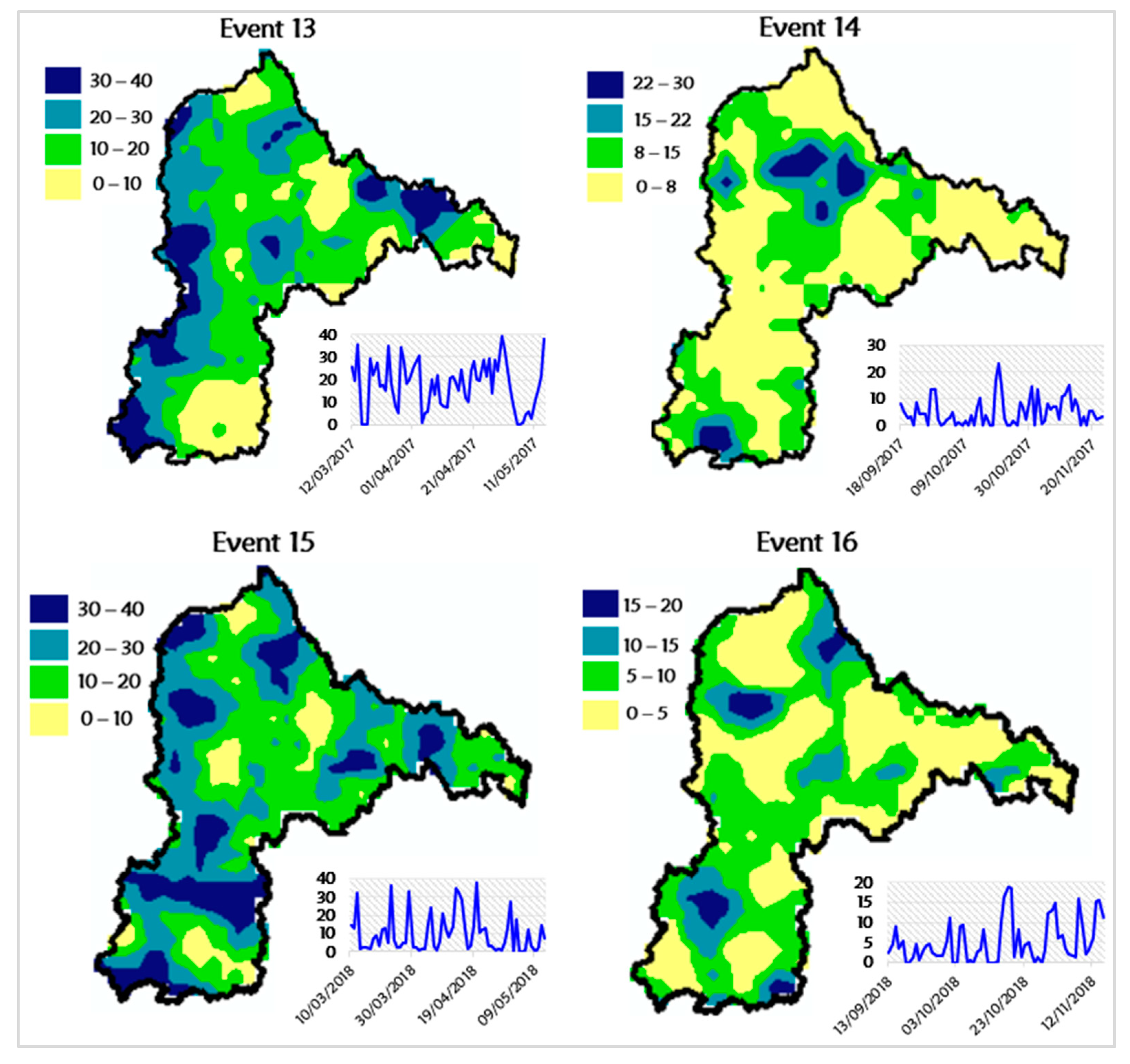
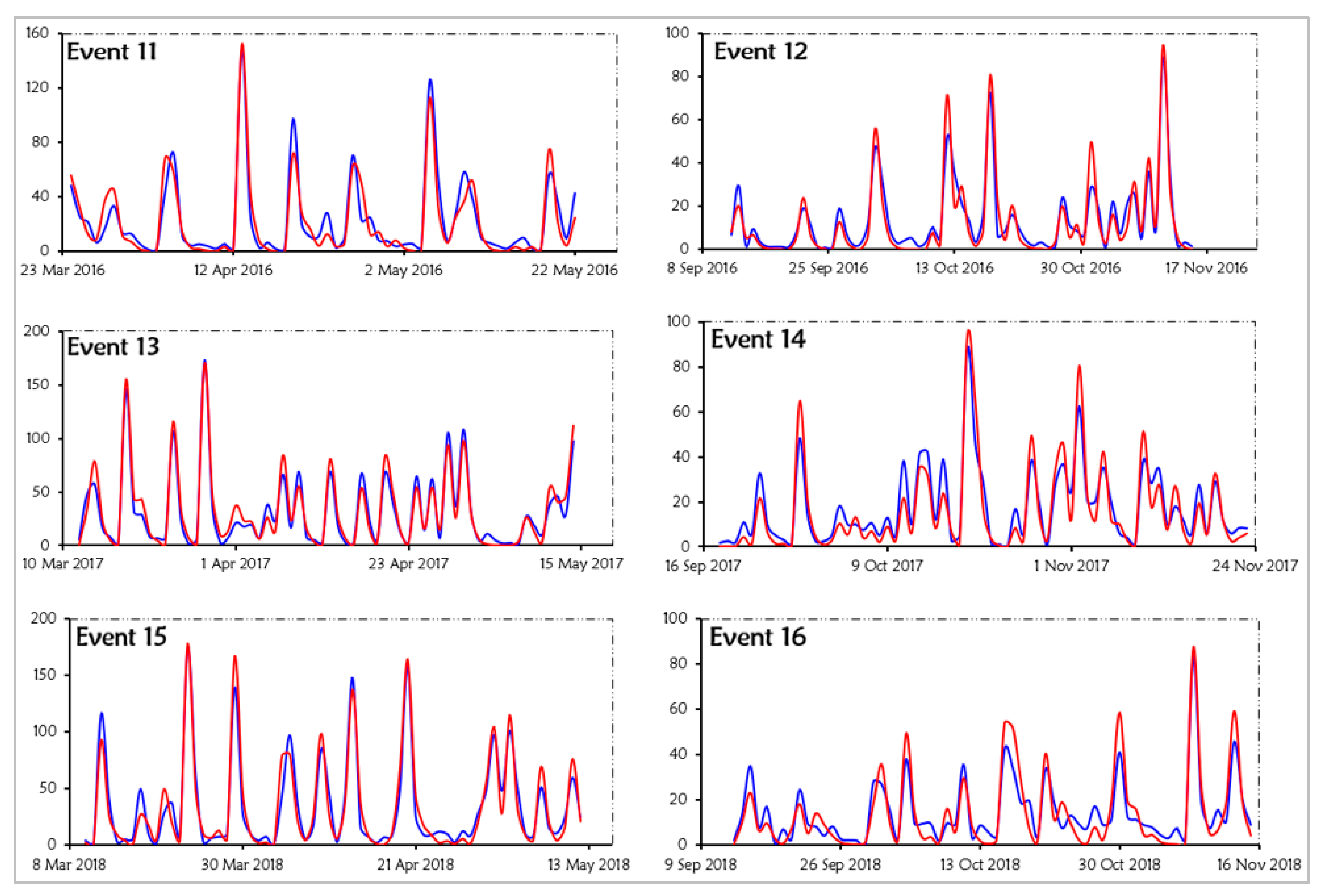
Generally, the results (Table 4 and Table 6) revealed a higher peak flow during the 15th, 9th, 13th, and 5th than in other events, with simulated values of 177.7 m³s⁻¹, 171.7 m³s⁻¹, 169.9 m³s⁻¹, and 166.9 m³s⁻¹, respectively. The latter were recognized as plausible compared to the amount of rainfall (hyetograph) received in their respective events (Figure 7); showing 2018, 2015, 2017 and 2013 as having high magnitudes of rainfall spells compared to the remaining periods. In line with this, recent studies conducted in East Africa revealed that it is obvious that with an increasing trend in rainfall variability, seasonal changes in the discharged flow are a possible outcome [95,96]. This can be said to be true in our case study, since the discharged flow fluctuations exhibited a notable relationship with rainfall variations following the rainy seasons; which also indicates a substantial influence of rainfall patterns on hydrological processes [97]. Moreover, existing studies revealed a great susceptibility of river catchments toward climatic variations [97,98,99,100]. In particular, these studies argued that temporal variations in rainfall patterns contribute to the modification of flow regimes and have a direct impact on discharged flow [99]. Thus, discharged flow peaks in rivers are prone to these types of variations, which can further lead to hydrometeorological-induced hazards such as flash floods. This study, therefore, suggests that flash flooding will likely increase across the Nyabarongo catchment, but that this will vary based on catchment characteristics and spatial changes in climate. This suggests a need for giving attention to vulnerable zones, particularly in built-up areas known to host many lives and properties at risk, with a lack of retention or strong drainage systems [49].

The plots of the observed over simulated flow hydrographs have been shown to follow a similar trend (Figure 8) and peak timing (Table S4). This confirmed the capability of the model to produce accurate predictions of discharged flows and volumes for different rainfall or flood events. However, it was generally evidenced that the land surface is soaked during the monsoon season, and it is known that rain falling in the catchment will flow as streamflow [99,100]. Thus, besides rainfall, the dynamic between non-climatic elements such as LULC and soil type might be a direct or indirect influencing driver for current and future discharged flow under biogeophysical mechanisms. On the other hand, since flow records lack the ability to combine irregularities in the catchment scale, real impacts can be better experimented on in flow modeling using global circulation models—a subject that is recommended for future exploration in this study area.

3.3. Statistical Tests for Accuracy and Performance of the Model

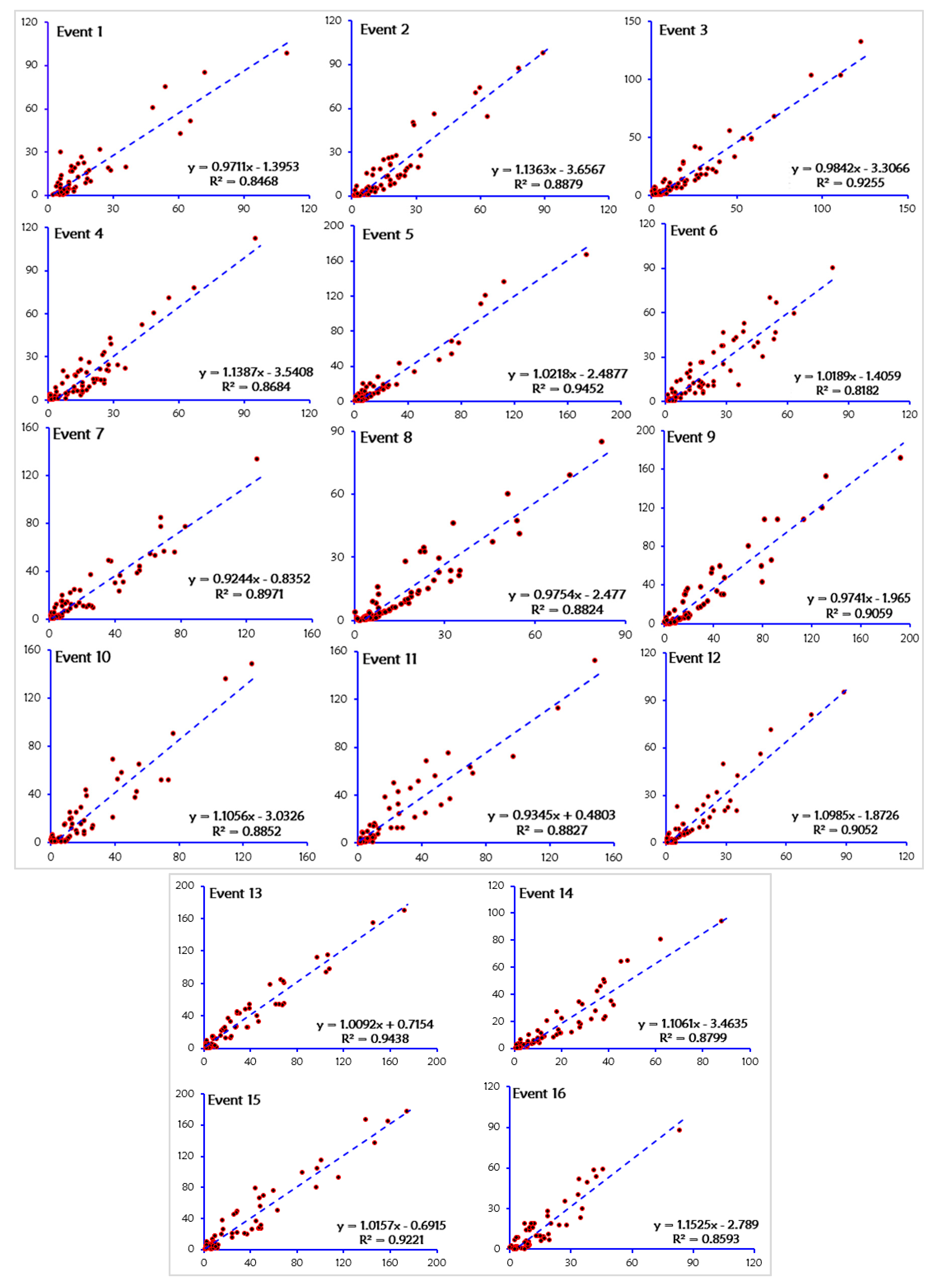
Conforming with recent studies [28,101], the relationships between the simulated and observed peak flow (Figure 9) have been calculated using different metrics for both calibration and validation processes. For instance, the correlation coefficient (R²) disclosed decent results (>80%) in all events, with an overall average of 88.4% and 89.8% for calibration and validation, respectively. Besides this, the NSE metric also exhibited satisfactory findings between the observed and simulated values, with an average of 80.9% and 84.6% for calibration and validation, respectively (Table 4 and Table 6). Statistically, lower acceptable average relative error percentages for all the events were also found for discharged flow (5.5% and 3.8%) and volume (7.7% and 4.6%) for calibration and validation, respectively. Overall, the model results have improved during the validation period using the optimized values. These findings are judged as being very much in agreement with the national criteria for flood forecasting in China, arguing that the rainfall–runoff model is considered effective when the error percentage of simulated volume is less than 20% [102]. Hence, HEC-HMS showed a better performance, computing efficacy, and predictive capability in simulating the discharged peak flow and volume for the Nyabarongo River catchment.

4. Conclusions

In this study, the discharged peak flow and volume simulation of the Nyabarongo River catchment in Rwanda were examined for corresponding rainfall events using a developed hydrological model and its algorithms, integrated with geospatial analyses. A total of sixteen events were selected covering the rainfall seasons, of which ten events were used for calibration and the remaining six used for validation at the catchment outlet. The performance evaluation of the model was determined using graphical and statistical approaches which revealed that the observed flow fitted well with the simulated discharged peak flow. After calibration and validation, the findings confirmed that the hydrological response of the Nyabarongo River catchment was directly associated with the rainfall seasons of Rwanda. Thus, with a slight increase in rainfall, there would be a risk of a surge in river flow which could consequently instigate widespread downstream flooding in the area.

In conclusion, HEC-HMS and its geospatial extension (HEC-GeoHMS) proved their capacity to simulate and estimate discharged flow based on different datasets and could, therefore, be used in other ungauged or poorly gauged adjacent catchments with similar features. The findings produced by this model could also be used as a decision support system in order to reduce downstream flooding risk in the catchment, as they can provide managers and decision-makers with vital information to help them take optimistic and effective initiatives for heavy rainfall-induced hazards. As a suggestion for such initiatives, the construction and design of drainage structures with sufficient conveyance capacity could be implemented in this area. Despite the good performance of the developed model, the study contains some limitations that cannot be disregarded in future research. For instance, one set of LULC data was used and no attention has been given to variations in land surface characteristics such as land use and soil properties, which have the potential to influence hydrological transformation within the catchment. Hence, the application of detailed hydrological models which integrate land-use change effects on hydrological processes may also improve the understanding and knowledge of current and future discharged flows. Owing to this, this study strongly recommends an investigation into the joint effects of non-climatic and climatic drivers on the hydrological response of the catchment. Moreover, due to the scarcity of long-term in-situ data, remote-sensing data with global circulation models can be taken into account to authenticate the drivers’ behavior, particularly for ungauged or poorly gauged catchments. Finally, more hydro-meteorological and weather stations must be established or revived across the country for future long-term assessments.

References

- Tabari, H. Climate change impact on flood and extreme precipitation increases with water availability. Sci. Rep. 2020, 10, 1–10. [Google Scholar] [CrossRef] [PubMed]
- Vondou, D.A.; Guenang, G.M.; Djiotang, T.L.A.; Kamsu-Tamo, P.H. Trends and Interannual Variability of Extreme Rainfall Indices over Cameroon. Sustainability 2021, 13, 6803. [Google Scholar] [CrossRef]
- Zafar, S.; Zaidi, A. Impact of urbanization on basin hydrology: A case study of the Malir Basin, Karachi, Pakistan. Reg. Environ. Chang. 2019, 19, 1815–1827. [Google Scholar] [CrossRef]
- Feng, B.; Zhang, Y.; Bourke, R. Urbanization impacts on flood risks based on urban growth data and coupled flood models. Nat. Hazards 2021, 106, 613–627. [Google Scholar] [CrossRef]
- Teklay, A.; Dile, Y.T.; Asfaw, D.H.; Bayabil, H.K.; Sisay, K. Impacts of Climate and Land Use Change on Hydrological Response in Gumara Watershed, Ethiopia. Ecohydrol. Hydrobiol. 2021, 21, 315–332. [Google Scholar] [CrossRef]
- Ma, D.; Qian, B.; Gu, H.; Sun, Z.; Xu, Y.P. Assessing climate change impacts on streamflow and sediment load in the upstream of the Mekong River basin. Int. J. Climatol. 2021, 41, 3391–3410. [Google Scholar] [CrossRef]
- Kumari, N.; Srivastava, A.; Sahoo, B.; Raghuwanshi, N.S.; Bretreger, D. Identification of suitable hydrological models for streamflow assessment in the Kangsabati River Basin, India, by using different model selection scores. Nat. Resour. Res. 2021, 1–19. [Google Scholar] [CrossRef]
- Mesta, B.; Akgun, O.B.; Kentel, E. Alternative solutions for long missing streamflow data for sustainable water resources management. Int. J. Water Resour. Dev. 2021, 37, 882–905. [Google Scholar] [CrossRef]
- Tassew, B.G.; Belete, M.A.; Miegel, K. Application of HEC-HMS model for flow simulation in the lake tana basin: The case of gilgel abay catchment, upper blue nile basin, Ethiopia. Hydrology 2019, 6, 21. [Google Scholar] [CrossRef]
- Tikhamarine, Y.; Souag-Gamane, D.; Ahmed, A.N.; Sammen, S.S.; Kisi, O.; Huang, Y.F.; El-Shafie, A. Rainfall-runoff modelling using improved machine learning methods: Harris hawks optimizer vs. particle swarm optimization. J. Hydrol. 2020, 589, 125133. [Google Scholar] [CrossRef]
- Dhital, Y.P.; Dawadi, B.; Kattel, D.B.; Devkota, K.C. Rainfall-runoff Simulation of Bagmati River Basin, Nepal. Jalawaayu 2021, 1, 61–71. [Google Scholar] [CrossRef]
- Brodie, I. An evaluation of a multi-day rainfall–runoff volume–peak discharge transform for flood frequency estimation. Australas. J. Water Resour. 2020, 24, 167–182. [Google Scholar] [CrossRef]
- Otim, D.; Smithers, J.; Senzanje, A.; van Antwerpen, R. Verification of runoff volume, peak discharge and sediment yield simulated using the ACRU model for bare fallow and sugarcane fields. Water SA 2020, 46, 182–196. [Google Scholar]
- Farrag, M.; Perez, G.C.; Solomatine, D. Spatio-Temporal Hydrological Model Structure and Parametrization Analysis. J. Mar. Sci. Eng. 2021, 9, 467. [Google Scholar] [CrossRef]
- Said, M.; Hyandye, C.; Mjemah, I.C.; Komakech, H.C.; Munishi, L.K. Evaluation and Prediction of the Impacts of Land Cover Changes on Hydrological Processes in Data Constrained Southern Slopes of Kilimanjaro, Tanzania. Earth 2021, 2, 225–247. [Google Scholar] [CrossRef]
- Fasipe, O.; Izinyon, O. Exponent determination in a poorly gauged basin system in Nigeria based on flow characteristics investigation and regionalization method. SN Appl. Sci. 2021, 3, 1–20. [Google Scholar] [CrossRef]
- Valles, J.; Corzo, G.; Solomatine, D. Impact of the Mean Areal Rainfall Calculation on a Modular Rainfall-Runoff Model. J. Mar. Sci. Eng. 2020, 8, 980. [Google Scholar] [CrossRef]
- Qiang, M.; Guomin, L.; Sijia, H.; Xiaoyan, Z.; Wenchuan, W.; Changjun, L. A New Generation Numerical Modelling Tool for Hydrological Simulation: Spatiotemporal-Varied-Source-Mixed Runoff Model for Small Watershed. In Proceedings of the 2021 International Conference on Control and Intelligent Robotics, Guangzhou, China, 18–20 June 2021; pp. 325–330. [Google Scholar]
- Revuelta-Acosta, J.; Flanagan, D.; Engel, B.; King, K. Improvement of the Water Erosion Prediction Project (WEPP) model for quantifying field scale subsurface drainage discharge. Agric. Water Manag. 2021, 244, 106597. [Google Scholar] [CrossRef]
- Yousuf, A.; Bhardwaj, A.; Prasad, V. Simulating the Impact of Conservation Interventions on Runoff and Sediment Yield in a Degraded Watershed Using the WEPP Model. Ecopersia 2021, 9, 191–205. [Google Scholar]
- Goudarzi, F.M.; Sarraf, A.; Ahmadi, H. Calibration of SWAT and three data-driven models for monthly stream flow simulation in Maharlu Lake Basin. Water Supply 2021. [Google Scholar] [CrossRef]
- Daneshvar, F.; Frankenberger, J.R.; Bowling, L.C.; Cherkauer, K.A.; Moraes, A.G.d.L. Development of strategy for SWAT hydrologic modeling in data-scarce regions of Peru. J. Hydrol. Eng. 2021, 26, 05021016. [Google Scholar] [CrossRef]
- Salviano, M.F.; Pereira Filho, A.J.; Vemado, F. TOPMODEL Hydrometeorological Modeling with Rain Gauge Data Integrated by High-Resolution Satellite Estimates. A Case Study in Muriaé River Basin, Brazil. Atmos. Clim. Sci. 2021, 11, 486–507. [Google Scholar]
- Beven, K.J.; Kirkby, M.J.; Freer, J.E.; Lamb, R. A history of TOPMODEL. Hydrol. Earth Syst. Sci. 2021, 25, 527–549. [Google Scholar] [CrossRef]
- Aredo, M.R.; Hatiye, S.D.; Pingale, S.M. Impact of land use/land cover change on stream flow in the Shaya catchment of Ethiopia using the MIKE SHE model. Arab. J. Geosci. 2021, 14, 114. [Google Scholar] [CrossRef]
- Zhang, J.; Zhang, M.; Song, Y.; Lai, Y. Hydrological simulation of the Jialing River Basin using the MIKE SHE model in changing climate. J. Water Clim. Chang. 2021, 12. [Google Scholar] [CrossRef]
- Gui, H.; Wu, Z.; Zhang, C. Comparative Study of Different Types of Hydrological Models Applied to Hydrological Simulation. CLEAN–Soil Air Water 2021, 2000381. [Google Scholar] [CrossRef]
- Hussain, F.; Wu, R.-S.; Yu, K.-C. Application of physically based semi-distributed HEC-HMS model for flow simulation in tributary catchments of Kaohsiung area Taiwan. J. Mar. Sci. Technol. 2021, 29, 4. [Google Scholar] [CrossRef]
- Ismail, H.; Kamal, M.R.; Hin, L.S.; Abdullah, A.F. Performance of HEC-HMS and ArcSWAT Models for Assessing Climate Change Impacts on Streamflow at Bernam River Basin in Malaysia. Pertanika J. Sci. Technol. 2020, 28, 1027–1048. [Google Scholar]
- Aliye, M.A.; Aliye, M.A.; Aga, A.O.; Tadesse, T.; Yohannes, P. Evaluating the Performance of HEC-HMS and SWAT Hydrological Models in Simulating the Rainfall-Runoff Process for Data Scarce Region of Ethiopian Rift Valley Lake Basin. Open J. Mod. Hydrol. 2020, 10, 105. [Google Scholar] [CrossRef]
- Xue, L.; Yang, F.; Yang, C.; Wei, G.; Li, W.; He, X. Hydrological simulation and uncertainty analysis using the improved TOPMODEL in the arid Manas River basin, China. Sci. Rep. 2018, 8, 452. [Google Scholar] [CrossRef] [PubMed]
- Thakur, J.K.; Singh, S.K.; Ekanthalu, V.S. Integrating remote sensing, geographic information systems and global positioning system techniques with hydrological modeling. Appl. Water Sci. 2017, 7, 1595–1608. [Google Scholar] [CrossRef]
- Maviza, A.; Ahmed, F. Climate change/variability and hydrological modelling studies in Zimbabwe: A review of progress and knowledge gaps. SN Appl. Sci. 2021, 3, 1–28. [Google Scholar] [CrossRef]
- Kumar, A.; Kanga, S.; Taloor, A.K.; Singh, S.K.; Đurin, B. Surface runoff estimation of Sind river basin using integrated SCS-CN and GIS techniques. HydroResearch 2021, 4, 61–74. [Google Scholar] [CrossRef]
- Zhou, Q.; Li, J. Geo-Spatial Analysis in Hydrology. ISPRS Int. J. Geo-Inf. 2020, 9, 435. [Google Scholar] [CrossRef]
- Khaddor, I.; Achab, M.; Hafidi Alaoui, A. Estimation of Peak Discharge in a Poorly Gauged Catchment Based on a Specified Hyetograph Model and Geomorphological Parameters: Case Study for the 23–24 October 2008 Flood, KALAYA Basin, Tangier, Morocco. Hydrology 2019, 6, 10. [Google Scholar] [CrossRef]
- Gatwaza, O.C. Impact of Urbanization on the Hydrological Cycle of Migina Catchment, Rwanda. Open Access Libr. J. 2016, 3, 1. [Google Scholar] [CrossRef]
- Paterne, N. Evaluating Drainage Systems Performance and Infiltration Enhancement Techniques as Flood Mitigation Measures in Nyabugogo Catchment, Rwanda. PAUSTI, JKUAT. 2019. Available online: http://ir.jkuat.ac.ke/bitstream/handle/123456789/4940/Niyonkuru%20Paterne-MSC%20MATHEMATICS-%202019.pdf?sequence=1&isAllowed=y (accessed on 13 February 2021).
- Manyifika, M. Diagnostic Assessment on Urban Floods Using Satellite Data and Hydrologic Models in Kigali, Rwanda; University of Twente: Enschede, The Netherland, 2015; Available online: http://essay.utwente.nl/84041/1/manyifika.pdf (accessed on 7 September 2021).
- Icyimpaye, G.; Abdelbaki, C.; Mourad, K.A. Hydrological and hydraulic model for flood forecasting in Rwanda. Model. Earth Syst. Environ. 2021, 1–11. [Google Scholar] [CrossRef]
- Ukurikiyeyezu, E. Spatial and Temporal Variability of Streamflow in Catchments Areas of Rwanda; University of Rwanda: Huye, Rwanda, 2018; Available online: http://hdl.handle.net/123456789/524 (accessed on 6 September 2021).
- Munyaneza, O.; Ufiteyezu, F.; Wali, U.; Uhlenbrook, S. A simple method to predict River flows in the agricultural Migina catchment in Rwanda. Nile Water Sci. Eng. J. 2011, 4, 24–36. [Google Scholar]
- Karamage, F.; Zhang, C.; Kayiranga, A.; Shao, H.; Fang, X.; Ndayisaba, F.; Nahayo, L.; Mupenzi, C.; Tian, G. USLE-based assessment of soil erosion by water in the Nyabarongo River Catchment, Rwanda. Int. J. Environ. Res. Public Health 2016, 13, 835. [Google Scholar] [CrossRef]
- Sendama, M.I. Assessment of Meteorological Remote Sensing Products for Stream Flow Modelling Using HBV-Light in Nyabarongo Basin, Rwanda; University of Twente: Enschede, The Netherland, 2015; Available online: http://essay.utwente.nl/84043/1/sendama.pdf (accessed on 6 September 2021).
- REMA. Rwanda State of Environment and Outlook; Government of Rwanda: Kigali, Rwanda, 2008. Available online: https://www.rema.gov.rw/soe/summary.pdf (accessed on 6 September 2021).
- Nteziyaremye, P.; Omara, T. Bioaccumulation of priority trace metals in edible muscles of West African lungfish (Protopterus annectens Owen, 1839) from Nyabarongo River, Rwanda. Cogent Environ. Sci. 2020, 6, 1779557. [Google Scholar] [CrossRef]
- Habiyakare, T.; Zhou, N. Water resources conflict management of Nyabarongo river and Kagera river watershed in Africa. J. Water Resour. Prot. 2015, 7, 889. [Google Scholar] [CrossRef]
- Sylvie, N. An Assessment of Farmers’ Willingness to Pay for the Protection of Nyabarongo River System, Rwanda; University of Nairobi: Nairobi, Kenya, 2012; Available online: https://ageconsearch.umn.edu/record/198529 (accessed on 6 September 2021).
- Mind’je, R.; Li, L.; Amanambu, A.C.; Nahayo, L.; Nsengiyumva, J.B.; Gasirabo, A.; Mindje, M. Flood susceptibility modeling and hazard perception in Rwanda. Int. J. Disaster Risk Reduct. 2019, 38, 101211. [Google Scholar] [CrossRef]
- Ndayisaba, F.; Guo, H.; Bao, A.; Guo, H.; Karamage, F.; Kayiranga, A. Understanding the spatial temporal vegetation dynamics in Rwanda. Remote Sens. 2016, 8, 129. [Google Scholar] [CrossRef]
- NewTimes. Govt, Private Sector Pledge to Conserve R. Nyabarongo. Available online: https://www.newtimes.co.rw/section/read/195536 (accessed on 13 September 2021).
- Tegegne, G.; Park, D.K.; Kim, Y.-O. Comparison of hydrological models for the assessment of water resources in a data-scarce region, the Upper Blue Nile River Basin. J. Hydrol. Reg. Stud. 2017, 14, 49–66. [Google Scholar] [CrossRef]
- Trinh, T.; Kavvas, M.; Ishida, K.; Ercan, A.; Chen, Z.; Anderson, M.; Ho, C.; Nguyen, T. Integrating global land-cover and soil datasets to update saturated hydraulic conductivity parameterization in hydrologic modeling. Sci. Total Environ. 2018, 631, 279–288. [Google Scholar] [CrossRef]
- Hamdan, A.N.A.; Almuktar, S.; Scholz, M. Rainfall-runoff modeling using the hec-hms model for the al-adhaim river catchment, northern iraq. Hydrology 2021, 8, 58. [Google Scholar] [CrossRef]
- Makki Vijayaprakash, P. Application of HEC-HMS modelling on River Storån, Model evaluation and analysis of the processes by using soil moisture accounting loss method. TVVR20/5021 2021. Available online: http://lup.lub.lu.se/student-papers/record/9035455 (accessed on 6 September 2021).
- Tesfamariam, E.G.; Home, P.G.; Gathenya, J.M. Rainfall-runoff modelling to determine continuous time series of daily streamflow in the Umba River, Kenya. Afr. J. Rural. Dev. 2021, 5, 49–68. [Google Scholar]
- Kang, M.; Yoo, C. Application of the SCS–CN Method to the Hancheon Basin on the Volcanic Jeju Island, Korea. Water 2020, 12, 3350. [Google Scholar] [CrossRef]
- Caletka, M.; Šulc Michalková, M.; Karásek, P.; Fučík, P. Improvement of SCS-CN initial abstraction coefficient in the Czech Republic: A study of five catchments. Water 2020, 12, 1964. [Google Scholar] [CrossRef]
- USDA. Hydrological Data for Experimental Agricultural Watersheds in the United States; USDA–ARS Miscellaneous Pub, US Gov. Print. Office Washington: Washington, DC, USA, 1967; pp. 945–1469. [Google Scholar]
- Song, X.-M.; Kong, F.-Z.; Zhu, Z.-X. Application of Muskingum routing method with variable parameters in ungauged basin. Water Sci. Eng. 2011, 4, 1–12. [Google Scholar]
- Ponce, V.M. Muskingum-Cunge Method Explained. 2020. Available online: http://jon.sdsu.edu/muskingum_cunge_method_explained.html. (accessed on 24 June 2021).
- Chow, V.T. Open-channel hydraulics. McGraw-Hill Civ. Eng. Ser. 1959. Available online: https://documentatiecentrum.watlab.be/imis.php?module=ref&refid=135703 (accessed on 11 October 2021).
- Attari, M.; Taherian, M.; Hosseini, S.M.; Niazmand, S.B.; Jeiroodi, M.; Mohammadian, A. A simple and robust method for identifying the distribution functions of Manning’s roughness coefficient along a natural river. J. Hydrol. 2021, 595, 125680. [Google Scholar] [CrossRef]
- Abbas, M.R.; Hason, M.M.; Ahmad, B.B.; Abbas, T.R. Surface roughness distribution map for Iraq using satellite data and GIS techniques. Arab. J. Geosci. 2020, 13, 839. [Google Scholar] [CrossRef]
- Tang, X.; Rahimi, H.; Guan, Y.; Wang, Y. Hydraulic characteristics of open-channel flow with partially-placed double layer rigid vegetation. Environ. Fluid Mech. 2021, 21, 317–342. [Google Scholar] [CrossRef]
- Wilson, B.N.; Ruffini, J.R. Comparison of physically-based Muskingum methods. Trans. ASAE 1988, 31, 91–0097. [Google Scholar] [CrossRef]
- Laouacheria, F.; Mansouri, R. Comparison of WBNM and HEC-HMS for runoff hydrograph prediction in a small urban catchment. Water Resour. Manag. 2015, 29, 2485–2501. [Google Scholar] [CrossRef]
- Saadi, M.; Oudin, L.; Ribstein, P. Physically consistent conceptual rainfall–runoff model for urbanized catchments. J. Hydrol. 2021, 599, 126394. [Google Scholar] [CrossRef]
- Hu, C.; Xia, J.; She, D.; Song, Z.; Zhang, Y.; Hong, S. A new urban hydrological model considering various land covers for flood simulation. J. Hydrol. 2021, 603, 126833. [Google Scholar] [CrossRef]
- Strohbach, M.W.; Döring, A.O.; Möck, M.; Sedrez, M.; Mumm, O.; Schneider, A.-K.; Weber, S.; Schröder, B. The “hidden urbanization”: Trends of impervious surface in low-density housing developments and resulting impacts on the water balance. Front. Environ. Sci. 2019, 7, 29. [Google Scholar] [CrossRef]
- Oudin, L.; Salavati, B.; Furusho-Percot, C.; Ribstein, P.; Saadi, M. Hydrological impacts of urbanization at the catchment scale. J. Hydrol. 2018, 559, 774–786. [Google Scholar] [CrossRef]
- Luo, J.; Zhou, X.; Rubinato, M.; Li, G.; Tian, Y.; Zhou, J. Impact of multiple vegetation covers on surface runoff and sediment yield in the small basin of Nverzhai, Hunan Province, China. Forests 2020, 11, 329. [Google Scholar] [CrossRef]
- Kroese, J.S.; Batista, P.; Jacobs, S.; Breuer, L.; Quinton, J.; Rufino, M. Agricultural land is the main source of stream sediments after conversion of an African montane forest. Sci. Rep. 2020, 10, 1–15. [Google Scholar] [CrossRef]
- Tram, V.N.Q.; Somura, H.; Moroizumi, T. The Impacts of Land-Use Input Conditions on Flow and Sediment Discharge in the Dakbla Watershed, Central Highlands of Vietnam. Water 2021, 13, 627. [Google Scholar] [CrossRef]
- Guha, S.; Govil, H.; Gill, N.; Dey, A. Analytical study on the relationship between land surface temperature and land use/land cover indices. Ann. GIS 2020, 26, 201–216. [Google Scholar] [CrossRef]
- Fischer, S.; Bühler, P.; Schumann, A. Impact of Flood Types on Superposition of Flood Waves and Flood Statistics Downstream. J. Hydrol. Eng. 2021, 26, 04021024. [Google Scholar] [CrossRef]
- Leng, M.; Yu, Y.; Wang, S.; Zhang, Z. Simulating the hydrological processes of a meso-scale watershed on the Loess Plateau, China. Water 2020, 12, 878. [Google Scholar] [CrossRef]
- Shen, Z.; Chen, L.; Chen, T. Analysis of parameter uncertainty in hydrological and sediment modeling using GLUE method: A case study of SWAT model applied to Three Gorges Reservoir Region, China. Hydrol. Earth Syst. Sci. 2012, 16, 121–132. [Google Scholar] [CrossRef]
- Arheimer, B.; Lindström, G. Climate impact on floods: Changes in high flows in Sweden in the past and the future (1911–2100). Hydrol. Earth Syst. Sci. 2015, 19, 771–784. [Google Scholar] [CrossRef]
- Kibria, K.N.; Ahiablame, L.; Hay, C.; Djira, G. Streamflow trends and responses to climate variability and land cover change in South Dakota. Hydrology 2016, 3, 2. [Google Scholar] [CrossRef]
- Khalil, A.; Rittima, A.; Phankamolsil, Y. Seasonal and Annual Trends of Rainfall and Streamflow in the Mae Klong Basin, Thailand. Appl. Environ. Res. 2018, 40, 77–90. [Google Scholar] [CrossRef]
- Vaghefi, S.A.; Keykhai, M.; Jahanbakhshi, F.; Sheikholeslami, J.; Ahmadi, A.; Yang, H.; Abbaspour, K.C. The future of extreme climate in Iran. Sci. Rep. 2019, 9, 1464. [Google Scholar] [CrossRef]
- Mamuye, M.; Kebebewu, Z. Review on impacts of climate change on watershed hydrology. Atmosphere 2018, 8. Available online: https://www.researchgate.net/publication/322977113_Review_on_Impacts_of_Climate_Change_on_Watershed_Hydrology (accessed on 6 September 2021).
- Tsegaw, A.T.; Pontoppidan, M.; Kristvik, E.; Alfredsen, K.; Muthanna, T.M. Hydrological impacts of climate change on small ungauged catchments-results from a GCM-RCM-hydrologic model chain. Nat. Hazards Earth Syst. Sci. Discuss. 2019, 2019, 1–56. [Google Scholar]
- MIDIMAR. The National Risk Atlas of Rwanda; The National Risk Atlas of Rwanda, Ed.; UNON: Nairobi, Kenya, 2015. [Google Scholar]
- Belayneh, A.; Sintayehu, G.; Gedam, K.; Muluken, T. Evaluation of satellite precipitation products using HEC-HMS model. Model. Earth Syst. Environ. 2020, 6, 2015–2032. [Google Scholar] [CrossRef]
- Zheng, Y.; Li, J.; Dong, L.; Rong, Y.; Kang, A.; Feng, P. Estimation of initial abstraction for hydrological modeling based on global land data assimilation system–simulated datasets. J. Hydrometeorol. 2020, 21, 1051–1072. [Google Scholar] [CrossRef]
- Namara, W.G.; Damise, T.A.; Tufa, F.G. Rainfall Runoff Modeling Using HEC-HMS: The Case of Awash Bello Sub-Catchment, Upper Awash Basin, Ethiopia. Int. J. Environ. 2020, 9, 68–86. [Google Scholar] [CrossRef]
- Chen, L.; Chen, S.; Li, S.; Shen, Z. Temporal and spatial scaling effects of parameter sensitivity in relation to non-point source pollution simulation. J. Hydrol. 2019, 571, 36–49. [Google Scholar] [CrossRef]
- Rahman, K.U.; Balkhair, K.S.; Almazroui, M.; Masood, A. Sub-catchments flow losses computation using Muskingum–Cunge routing method and HEC-HMS GIS based techniques, case study of Wadi Al-Lith, Saudi Arabia. Model. Earth Syst. Environ. 2017, 3, 4. [Google Scholar] [CrossRef]
- Yin, J.; He, F.; Xiong, Y.J.; Qiu, G.Y. Effects of land use/land cover and climate changes on surface runoff in a semi-humid and semi-arid transition zone in northwest China. Hydrol. Earth Syst. Sci. 2017, 21, 183–196. [Google Scholar] [CrossRef]
- Yang, K.; Lu, C. dEvaluation of land-use change effects on runoff and soil erosion of a hilly basin—The Yanhe River in the Chinese Loess Plateau. Land Degrad. Dev. 2018, 29, 1211–1221. [Google Scholar] [CrossRef]
- Zhang, D.; Lin, Q.; Chen, X.; Chai, T. Improved curve number estimation in SWAT by reflecting the effect of rainfall intensity on runoff generation. Water 2019, 11, 163. [Google Scholar] [CrossRef]
- Kumar, P.; Sherring, A. Modelling of rainfall and runoff using HEC-HMS in Oghani Micro-watershed of Azamgarh District Uttar Pradesh. IJCS 2021, 9, 3476–3482. [Google Scholar]
- Twisa, S.; Buchroithner, M.F. Seasonal and Annual Rainfall Variability and Their Impact on Rural Water Supply Services in the Wami River Basin, Tanzania. Water 2019, 11, 2055. [Google Scholar] [CrossRef]
- Langat, P.K.; Kumar, L.; Koech, R. Temporal variability and trends of rainfall and streamflow in Tana River Basin, Kenya. Sustainability 2017, 9, 1963. [Google Scholar] [CrossRef]
- Ran, Q.; Wang, F.; Gao, J. Modelling effects of rainfall patterns on runoff generation and soil erosion processes on slopes. Water 2019, 11, 2221. [Google Scholar] [CrossRef]
- Maharjan, M.; Aryal, A.; Talchabhadel, R.; Thapa, B.R. Impact of Climate Change on the Streamflow Modulated by Changes in Precipitation and Temperature in the North Latitude Watershed of Nepal. Hydrology 2021, 8, 117. [Google Scholar] [CrossRef]
- Lapides, D.A.; Leclerc, C.D.; Moidu, H.; Dralle, D.N.; Hahm, W.J. Variability of stream extents controlled by flow regime and network hydraulic scaling. Hydrol. Process. 2021, 35, e14079. [Google Scholar] [CrossRef]
- Khoi, D.N.; Loi, P.T.; Sam, T.T. Impact of Future Land-Use/Cover Change on Streamflow and Sediment Load in the Be River Basin, Vietnam. Water 2021, 13, 1244. [Google Scholar] [CrossRef]
- Shah, M.; Lone, M. Hydrological modeling to simulate stream flow in the Sindh Valley watershed, northwest Himalayas. Model. Earth Syst. Environ. 2021, 1–10. [Google Scholar] [CrossRef]
- Wang, W.-C.; Zhao, Y.-W.; Chau, K.-W.; Xu, D.-M.; Liu, C.-J. Improved flood forecasting using geomorphic unit hydrograph based on spatially distributed velocity field. J. Hydroinform. 2021, 23, 724–739. [Google Scholar] [CrossRef]
Figure 1.
Geographical location map of the Nyabarongo River catchment; (a) Location at the continent level; (b) Location at the country level; (c) An aerial outlook of the Nyabarongo River [51]; (d) Normalized difference vegetation index of the catchment with the Nyabarongo River and lakes.
Figure 2.
(a) LULC, (b) soil properties and hydrological Soil Groups (HSG), (c) CNgrid.
Figure 3.
Input geospatial datasets from terrain preprocessing for catchment delineation: (a) Reconditioned DEM; (b) Streams; (c) Filled sinks; (d) Slope; (e) Flow direction; (f) Flow accumulation; (g) Defined stream segmentation and drainage points; (h) Catchment grid delineation.
Figure 4.
Methodological flow design representing the procedures for the HEC-HMS model.
Figure 5.
Basin model with topological connections between catchment features determining flow connectivity (designed using ArcGIS and HEC-HMS software) while the numbers in brackets represent the subbasins.
Figure 6.
Comparison between the simulated and observed flow hydrographs (calibration events).
Figure 7.
Rainfall hyetographs distribution per event.
Figure 8.
Simulated and observed flow hydrographs for the events (validation).
Figure 9.
Relationships between simulated and observed flow for calibration and validation.