Soft Data in Hydrologic Modeling: Prediction of Ecologically Relevant Flows with Alternate Land Use/Land Cover Data

Abstract

Watershed-scale hydrological models have become important tools to understand, assess, and predict the impacts of natural and anthropogenic-driven activities on water resources. However, model predictions are associated with uncertainties stemming from sources such as model input data. As an important input to most watershed models, land use/cover (LULC) data can affect hydrological predictions and influence the interpretation of modeling results. In addition, it has been shown that the use of soft data will further ensure the quality of modeling results to be closer to watershed behavior. In this study, the ecologically relevant flows (ERFs) are the primary soft data to be considered as a part of the modeling processes. This study aims to evaluate the impacts of LULC input data on the hydrological responses of the rapidly urbanizing Upper Cahaba River watershed (UCRW) located in Alabama, USA. Two sources of LULC data, i.e., National Land Cover Database (NLCD) and Digitized Landsat 5 Thematic Mapper (TM) images, were used as input in the Soil and Water Assessment Tool (SWAT) model for the years 1992 and 2011 using meteorological data from 1988 to 2013. The model was calibrated at the watershed outlet against daily streamflow from 1988 to 1993 using the 1992 LULC data and validated for the 2008–2013 period using the 2011 LULC datasets. The results show that the models achieved similar performances with both LULC datasets during the calibration and validation periods according to commonly used statistical rating metrics such as Nash Sutcliffe efficiency coefficient (NSE), coefficient of determination (R²), and model percent bias (PBIAS). However, LULC input information had substantial impacts on simulated ERFs such as mean monthly streamflow, maximum and minimum flows of different durations, and low flow regimes. This study demonstrates that watershed models based on different sources of LULC and applied under different LULC temporal conditions can achieve equally good performances in predicting streamflow. However, substantial differences might exist in predicted hydrological regimes and ERF metrics depending on the sources of LULC data and the LULC year considered. Our results reveal that LULC data can significantly impact the simulated flow regimes of the UCRW with underlaying influences on the predicted biotic and abiotic structures of aquatic and riparian habitats.

1. Introduction

Hydrologic models have been widely used to assess the interplays between land use/cover (LULC) changes and hydrological processes and play a pivotal role in regulatory, planning, research, and decision-making efforts [1,2]. However, the simulated hydrologic fluxes and processes contain uncertainties from various sources since hydrologic models are essentially a simplified representation of natural systems [3]. Model predictive uncertainties can be attributed to forcing data (e.g., time-series of precipitation), input parameters (e.g., parameterization of soil physical properties), and an oversimplified model structure and representation of hydrologic processes (e.g., streamflow) [4,5,6].

Studies such as [4,7,8] examined the parameter uncertainty stemming from different LULC conditions and indicated substantial model output uncertainties. When developing a mathematical model of a physical system, such as a river basin, there may be multiple model structures and many different parameter combinations satisfying the description of the system equally well [9]. This has been referred to as the equifinality concept. Equifinality originates from inadequate model constraints that when combined with overparameterized models, results in a scenario where the number of unknown parameters surpasses the number of observations of the system [3]. In other words, it means that different sets of model parameters may yield similar outcomes for an observed signal, such as streamflow at the watershed outlet, while producing entirely different spatial responses of other hydrological processes (e.g., evapotranspiration). This becomes an issue since the larger the number of parameter combinations producing equally good model performance in predicting a given process (e.g., discharge), the less confidence the modeler will have in electing a single parameter set, especially if they yield completely different watershed responses [10].

A challenging trend that could impact model parameterization and increase model uncertainty and equifinality nowadays is the abundance of datasets of varying spatial and temporal resolutions, many of which have not been sufficiently tested for specific regions [11]. Frequently, modelers accept the available input data as free of errors and ignore the uncertainty stemming from input data [12]. Since inadequate and low-quality input data (e.g., overly coarse resolution of precipitation data) may produce unrealistic parameter values and lead to inaccurate model outputs, it is vital to evaluate model performances using different datasets [11]. A key input dataset required by most watershed models is the land use/cover of the watershed. The LULC map is a categorical geospatial data layer that provides the types (categories) and coverage (number of pixels per category) of land uses in the watershed [5]. Watershed modeling needs accurate LULC datasets to parameterize the physical system realistically. Therefore, LULC datasets are crucial inputs for assigning parameters related to the watershed hydrology since several hydrological processes (e.g., surface runoff and lateral flow) in a watershed highly depend on the type and extent of LULC [5].

Multiple studies have shown relatively low impacts of LULC input data on simulated streamflow when the model assessment is solely based on widely used model performance metrics, such as Nash Sutcliffe Efficiency (NSE), coefficient of determination (R²), and model percent bias (PBIAS), and evaluation criteria such as the ones proposed by [13,14,15,16,17,18]. However, significant influences have been found on water quality predictions and other components of the watershed water budget. [19] demonstrated that the LULC data resolution greatly impacts sediment, nitrate (NO₃⁻), and total phosphorus (T.P.). In a similar study, [20] showed that different LULC datasets substantially impacted simulated monthly ammonium (NH₄⁺) and T.P. loads. [11] found that runoff seems to be less sensitive to different LULC sources, whereas LULC data have significant impacts on different components of the water balance, such as soil water content and ET.

The main focus in most of the past studies was on the effects of LULC datasets on basic hydrologic characteristics such as mean annual/monthly flows and model performance based on widely used metrics (e.g., NSE). To the best of the author’s knowledge, no study has investigated the influence of different LULC data sources on ecologically relevant flows (ERFs) parameters and their consequences for river biodiversity and aquatic habitats. The very same concept can also be referred as “Soft Data” or “Interior Watershed Processes”, which are the essential nontemporal data used in modeling processes such as the denitrification rate, or ERFs in this study [6]. Many times, complex watershed dynamics might not be properly reflected by only considering temporal data or hard data (e.g., daily flow, monthly sediment load, etc.) in calibration/validation routines [21]. Therefore, the proposed work will strengthen the scientific credibility of the corresponding modeling results. In cases where temporal data are not available, soft data can also be used as the primary measurement data for model calibration/validation. River biodiversity and ecosystem are strongly associated with the flow regime, which regulates aquatic and riparian environments [22]. The flow regime plays a core role in the biotic composition, structure, and dynamics of river ecosystems [23]. For instance, the natural biodiversity and stability of aquatic ecosystems highly depend on the magnitude, frequency, timing, duration, and alteration of in-stream fluxes [24]. Overall, streamflow is one of the most critical abiotic drivers of the occurrence and distribution of freshwater biota [25]. Many riverine species, such as fish, benthic macroinvertebrates, and phytoplankton, have developed specific adaptions to flow conditions and thus are impacted by streamflow alterations [26]. Thus, even small or moderate changes in discharge may have consequences to aquatic environments. Since watershed models have been increasingly used to investigate the impacts of anthropogenic changes on water resources and considering that LULC data are a key input to most models, it is important to investigate how LULC information can impact the ecosystem. However, the assessment of the importance and impacts of LULC data on ERF, such as high flows, lows flows, and frequency and duration of extreme flows, is sorely lacking in watershed modeling studies.

In this study, we consider input data uncertainty stemming from different LULC data sources in the Soil and Water Assessment Tool (SWAT) [27] model. The objective is to assess the impacts of LULC data and associated uncertainty on ERF metrics. Our purpose is not to identify the best LULC dataset. What particularly interests us is to investigate an unexplored scientific question: How do hydrological models that were set up based on different sources of LULC data respond in terms of ERF conditions? Specifically, we aim to address the following related questions: (i) If LULC data from different sources are used as model input data, is it possible to achieve equally good model performances in streamflow prediction through automated model calibration? (ii) If yes, would those models predict similar streamflow under future LULC? (iii) What is the impact of different LULC data sources on ERF metrics? To answer these questions, we employed the SWAT model in an urbanizing watershed with high biodiversity, the Upper Cahaba River Watershed in Alabama, USA. SWAT-generated time series of daily discharge were used as input to the Indicators of Hydrologic Alterations Software (IHA) [23,28] to assess the impacts of LULC data on ERF metrics.

2. Materials and Methods

2.1. Study Area

This study focuses on the Upper Cahaba River watershed (UCRW) (1416 km²), which is part of the Cahaba River watershed, located in central Alabama, USA (Figure 1). The Cahaba River is one of the main tributaries of the Alabama River, which drains into the Mobile Bay, the fourth largest estuary in the U.S in terms of freshwater inflow [29]. The Cahaba River extends for 307 km from its source, near Trussville in St. Clair County, south to the Alabama River, and its drainage area lies entirely within Alabama. According to the Nature Conservancy, the Cahaba River and its major tributaries support 69 rare and imperiled species, making it one of the most diverse aquatic ecosystems in the United States [30]. The upper side of the Cahaba River watershed drains a large part of the city of Birmingham, AL. As a result of the expansion of the Birmingham metropolitan area, the percentage of urban areas within the UCRW increased from 9.3% (1992 NLCD) to 35.7% (2011 NLCD) (

Table 1. Land use/cover classes and changes in the Upper Cahaba River watershed.

Categories	1992		2011
LULC classes	NLCD (%)	DIGITIZED (%)	NLCD (%)	DIGITIZED (%)
Water	1.1	0.9	1.4	0.9
Urban	9.3	10.0	35.7	48.0
Forest	78.4	71.3	50.3	45.4
Agriculture	9.0	14.4	10.3	4.5
Wetland	1.3	3.0	1.9	0.7

). The climate (

Table 2. Characteristics of the Upper Cahaba River watershed.

Physical Characteristic
Maximum Elevation (meters)	459
Minimum Elevation (meters)	24
Area (km2)	1416
Mean Annual Precipitation (1950–2014) (mm)	1429
Mean Annual Average Temperature (1950–2014) (°C)	16.9

) is mainly humid, with a mean annual rainfall of 1429 mm. Mean rainfall is typically higher during the spring and winter and slightly lower during the summer and fall. The mean monthly minimum and maximum temperatures in the UCRW range from approximately 10.4 °C to 23.4 °C, respectively (NOAA, 1 January 1950–31 December 2014).

Due to rapid urbanization rates observed in the last few decades, the UCRW has witnessed fluctuations in flow regime with underlying effects on the aquatic and riparian biota [31,32,33]. This reality, combined with the watershed’s remarkable biodiversity, makes the UCRW an ideal test case to study the impacts of LULC data source on simulated ERF metrics.

2.2. Watershed Model

The SWAT model is a semi-physically based, continuous-time, hydrological, and agricultural management practice simulation model that assesses impacts of land management practices on water quantity and quality in complex watersheds [27]. SWAT runs at daily or sub-daily time step depending on the infiltration method used and can perform continuous simulations over very long periods [34,35]. It is suitable to evaluate the long-term influence of land management practices on water, sediment, and agricultural chemical yields in heterogeneous watersheds with varying land use, soil, and management conditions [27,36]. SWAT is among the most widely used watershed models worldwide [37] and has been applied in addressing a variety of flow and water quality problems [37].

To characterize spatial heterogeneity, SWAT requires watersheds divided into subwatersheds. Based on unique combinations of land use, soils, and slope characteristics, each subwatershed is split into multiple hydrological response units (HRUs). Beyond affecting the watershed configuration, LULC information influences many processes simulated in SWAT (e.g., canopy interception and evapotranspiration in the Penman–Monteith formulation, runoff generation and infiltration, overland flow routing, management operations) [30]. The surface runoff in each subwatershed was estimated based on the SCS-CN curve number method (the standard method utilized in SWAT for surface runoff generation) using the plant evapotranspiration method to calculate daily CN values. The estimated runoff volume was routed from the subwatersheds to the main channel using the Muskingum routing method [38]. The SCS-CN method is formulated as follows:

$$Q_{surf}=\frac{{\left(R_{day}-I_a\right)}^2}{\left(R_{day}-I_a+S\right)}$$

(1)

where $Q_{surf}$ is the daily surface runoff (mm), $R_{day}$ is the daily rainfall (mm), $I_a$ is the initial abstractions term (mm) (commonly calculated as 0.2S), and S is the potential maximum retention of water by soils. The retention parameter is defined as:

$$S=\frac{25400}{CN}-254$$

(2)

where CN is the curve number for the day. The SCS curve number is a function of the soil’s permeability, land use, and antecedent soil moisture conditions. Typical curve number values for various land covers and soil types were compiled by the SCS Engineering Division and can be easily found in most hydrology books.

SWAT includes three built-in methods for estimating potential evapotranspiration (PET) (i.e., Hargreaves, Priestley–Taylor, and Penman–Monteith) and allows the user to provide PET values calculated using different methods. In the current study, we use the Penman–Monteith method to estimate daily PET. For detailed information about the Penman–Monteith method and SWAT hydrological computations, readers are referred to SWAT’s theoretical manual [32].

2.3. Model Setup and Input Data

The geographic information system interface ArcSWAT 2012.10.18 was used to parametrize the SWAT model for the UCRW. The watershed was delineated from a 10-m-resolution DEM (https://gdg.sc.egov.usda.gov, accessed on 17 June 2015). The outlet was selected 27 km downstream of the United States Geological Survey (USGS) site 02423500 gage to capture the Northwest branch joining the Cahaba River near the outlet (Figure 1) and examine the portion of the watershed draining the Birmingham metropolitan area.

The daily precipitation and maximum/minimum air temperature data were obtained from the spatial climate gridded dataset (4 km cell resolution) of PRISM Climate Group (http://prism.oregonstate.edu, accessed on 20 August 2015). The remaining weather forcing data were obtained from the National Centers for Environmental Prediction (NCEP) Climate Forecast System Reanalysis (CFSR) database (http://rda.ucar.edu, accessed on 21 August 2015).

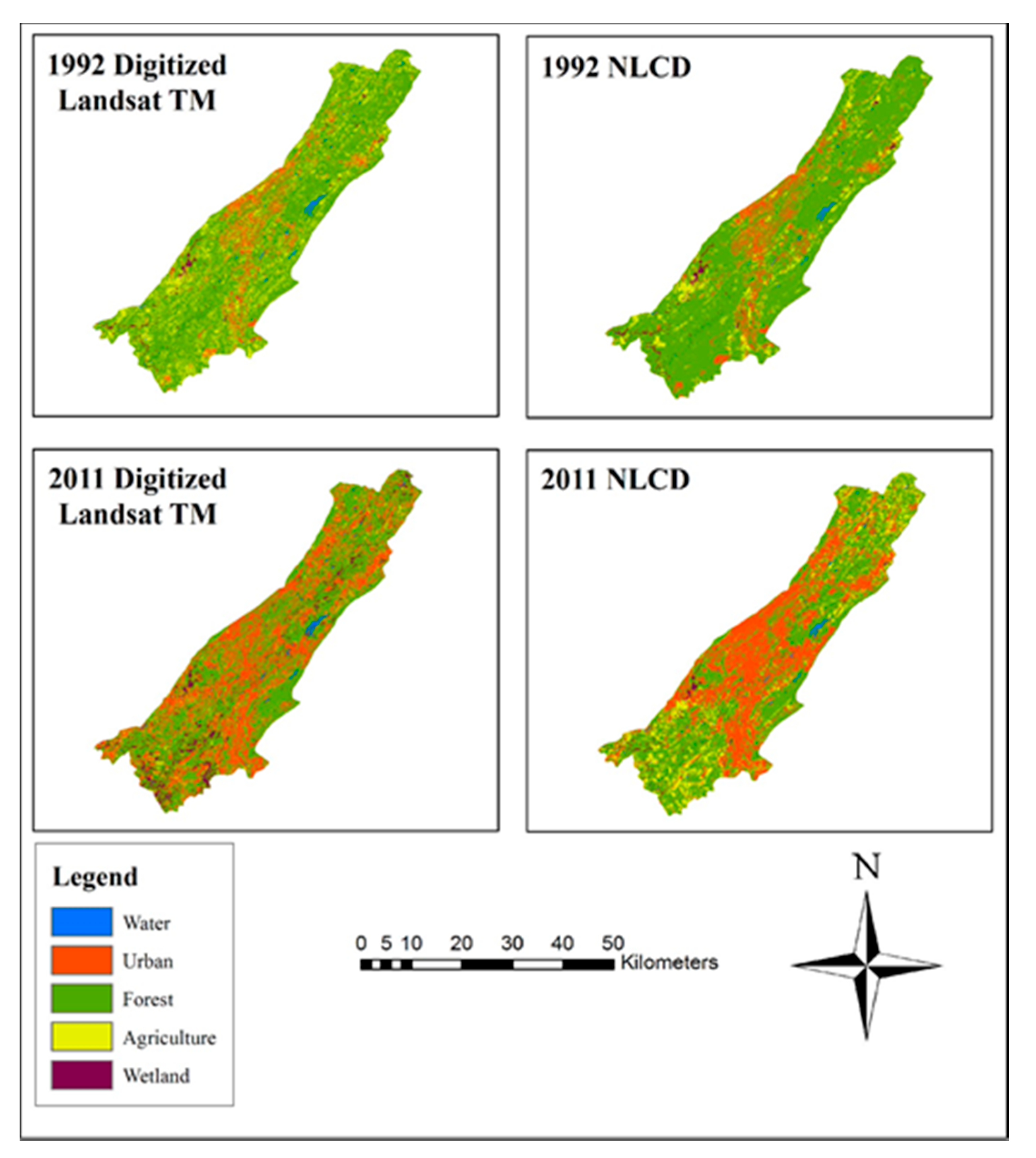
The impacts of the LULC change on hydrology and ERF were studied through two different LULC data sources (Figure 2). The National Land Cover Database (NLCD) is a publicly available dataset at 30 m resolution (available at: http://www.mrlc.gov/, accessed on 12 June 2015). We used the NLCD maps for the years 1992 and 2011. The second dataset was digitized from Landsat 5 TM scenes for the years 1992 and 2011. Since the NLCD LULC classes differed from those of the digitized maps, a reclassification process was applied to the Anderson Level II NLCD LULC maps. In order to be compatible with the digitized LULC classification, the original NLCD LULC classes were aggregated into the broader categories (Anderson Level I) according to the following criteria: Water = Water; Urban = Develop, Open Space + Developed Low Density + Developed Medium Density + Developed High Density; Forest = Deciduous Forest + Evergreen Forest + Mixed Forest; Agriculture = Pasture/Hay + Cultivated Crops; Wetland = Woody Wetlands + Emergent Herbaceous Wetlands.

The watershed soil map and soil properties needed to parameterize SWAT’s soil database were obtained from the SSURGO database (https://gdg.sc.egov.usda.gov, accessed on 17 July 2015). The average soil texture in the UCRW is 67.2% sand, 17.5% clay, and 15.3% silt.

The daily measured discharge data for the period 1983–2013 were obtained from the USGS National Water Information System website (http://waterdata.usgs.gov/nwis, accessed on 21 August 2015) for gauging station 02423500 (Figure 1). The daily discharge time series was used for model calibration (1988–1993) and validation (2008–2013). The 1992 and 2011 LULC maps were used during calibration and validation, respectively. The input data utilized to set up the UCRW model and the sources are summarized in

Table 3. Input data used in the SWAT model and data sources.

Input Data	Data Source	References
LULC map	NLCD and Digitized Landsat 5	National Land Cover Database (NLCD): http://www.mrlc.gov/, accessed on 12 June 2015
Landsat TM images	USGS	http://earthexplorer.usgs.gov/, accessed on 12 June 2015
Soil map (SSURGO)	USDA	USDA The Geospatial Data Gateway: https://gdg.sc.egov.usda.gov/, accessed on 17 July 2015
DEM	USDA (10 m)	USDA The Geospatial Data Gateway: https://gdg.sc.egov.usda.gov/, accessed on 17 July 2015
Measured daily streamflow	USGS	USGS National Water Information System: http://waterdata.usgs.gov/, accessed on 21 August 2015
Daily climate data (precipitation, minimum and maximum temperature, solar radiation, wind speed, relative humidity)	PRISM and CFRS	PRISM Climate Group: http://prism.oregonstate.edu/, accessed on 20 August 2015 NCEP Climate Forecast System Reanalysis (CFRS): http://rda.ucar.edu/, accessed on 21 August 2015

.

Based on the described data, the watershed was discretized into 45 sub-basins, with 557 and 540 HRUs for the 1992 and 2011 NLCD LULC datasets, respectively. Similarly, 713 and 614 HRUs were created for the 1992 and 2011 digitized LULC, respectively. In the current study, we use the multiple HRUs option in ArcSWAT and discretize the sub-basins into HRUs using an 8–8–10% threshold of land use, soil, and slope, respectively. In other words, land uses and soil types that covered less than 8% of the subbasin area were eliminated. The same applied to slopes covering less than 10% of the subbasin. After the elimination process, the remaining areas were reapportioned so that 100% of subbasin area was considered [39].

2.4. LULC Data Generation from Satellite Images

We utilized the Landsat 5 Thematic Mapper (TM) data (30 m spatial resolution) for 1992 and 2011 to derive alternative land use maps based on a supervised classification methodology in ERDAS IMAGINE 2015 software. The dates of both images were selected to be as close as possible and encompass the same vegetation season.

Five land use classes were generated: (1) Water, (2) Urban, (3) Forest, (4) Agriculture, (5) Wetland. This step was performed by launching the signature editor and then drawing polygons over the relevant features within the specified study area. The new classes were created from the drawn polygons with “signature editor”. Pixels were collected for urban areas from many different parts of the satellite image to enhance the spatial heterogeneity of the final product and avoid polygons clustered around a specific region. After a substantially large number of pixels spatialized across the watershed area were sampled, the new classes were created within the signature editor. Next, meaningful names and colors were assigned to each land use category. To overcome the limitation of choosing vegetative areas in some regions, the Normalized Difference Vegetation Index (NDVI) was also used to yield the image with pixel values ranging from −1 to +1. With the NDVI, the vegetative areas were analyzed successfully. For example, where Red reflectance exceeded Near-Infrared reflectance (NIR), negative values occurred on the map. Therefore, NDVI values ranging from −1 to 0 essentially indicated no vegetation cover. The False Color Composite of the Landsat TM scenes (1992 and 2011) was used for the accuracy assessment of both land use datasets.

2.5. Model Calibration, Validation, and Performance Assessment

Many hydrological models contain parameters that cannot be determined directly from field measurements, remote sensing, or environmental databases. SWAT incorporates a vast number of parameters, and therefore, identifying that the most sensitive ones can increase the calibration efficiency. In this study, global sensitivity analysis and calibration were independently carried out for the models developed with 1992-NLCD and 1992-Digitized LULC maps, using the SWAT Calibration and Uncertainty Program (SWAT-CUP) [40] through the Sequential Uncertainty Fitting (SUFI-2) algorithm and involved a total of 16 SWAT parameters (

Table 4. Calibrated model parameters and fitted values for each LULC dataset.

Variation *	Parameter	Parameter Definition	Absolute Ranges	Default SWAT Values	Fitted Value
					NLCD	Digitized
(r)	CN2	Initial SCS CN II Value	35–98	Varies **	−0.22	−0.19
(v)	CANMX	Maximum canopy storage	0–100	0	64.42	53.18
(v)	GW_REVAP	Groundwater “revap” coefficient	0.02–2	0.02	0.033	0.052
(r)	SOL_K	Saturated hydraulic conductivity (mm/h)	0–2000	100.8	−0.29	−0.44
(v)	GW_DELAY	Groundwater delay (days)	0–500	31	26.83	12.56
(r)	RCHRG_DP	Deep aquifer percolation fraction	0–1	0.05	0.28	0.24
(v)	GWQMN	Threshold depth of water in the shallow aquifer (mm)	0–5000	1000	387.25	374.61
(r)	SOL_BD	Moist bulk density (g/cm3)	0.9–2.5	1.45	0.14	0.08
(v)	GWHT	Initial groundwater height (m)	0–25	1	3.11	3.68
(v)	ALPHA_BNK	Baseflow alpha factor for bank storage	0–1	0	0.50	0.56
(v)	SURLAG	Surface runoff lag time	0.05–24	4	15.34	15.43
(v)	ESCO	Soil evaporation compensation factor	0–1	0.95	0.30	0.21
(v)	REVAPMN	Threshold depth of water in the shallow aquifer for “revap” (mm)	0–500	1	299.10	219.46
(r)	SOL_AWC	Available water capacity of the soil layer	0–1	0.15	0.16	0.31
(v)	EPCO	Plant uptake compensation factor	0–1	1	0.58	0.52
(v)	ALPHA_BF	Baseflow alpha factor (days)	0–1	0.048	0.37	0.44

* (r) means an existing parameter value is multiplied by (1+ a given value), and (v) means the existing parameter value is to be replaced by given value. ** varies by soil and LULC type.

). In SUFI-2, parameter sensitivity is computed by quantifying the average change in the defined objective function resulting from changes in each parameter [40]. The p-value tests the null hypothesis that the coefficient of a parameter is equal to zero (i.e., the parameter is not sensitive). Low p-values (typically <0.05) indicate sensitive parameters.

The calibrated model parameters were selected based on previous modeling efforts [30], sensitivity analysis results, the physical characteristics of the study area (e.g., forest coverage, extent of impervious areas), and their role in the computation of hydrologic processes in SWAT [36].

To calibrate and validate the 1992-NLCD and 1992-Digitized LULC based SWAT models, daily measured discharge records from the USGS 02423500 gage station for 1983–2013 were split into calibration (1988–1993) and validation (2008–2013) periods with three years of warmup in each period. The calibration and validation periods were selected to be close to the periods represented by the LULC datasets utilized. During the model calibration stage, SWAT was set up using 1992-NLCD and 1992-Digitized LULC data. Similarly, 2011 NLCD and 2011 Digitized LULC datasets were utilized during the validation period. The best parameter values found through the calibration process were transferred to the models employed during the validation period. The same soil data were used during model calibration and validation.

For assessing model performances, the coefficient of determination (R²), Nash–Sutcliffe Efficiency (NSE), and percent bias (PBIAS) were used. These are commonly used rating metrics to evaluate the performance of hydrologic models [14,41,42].

2.6. Ecologically Relevant Flow Estimation

To investigate the degree of hydrologic alteration attributable to LULC input information in hydrologic models, we utilized the Indicators of Hydrologic Alterations (IHA) tool [28]_. The IHA was developed by the Nature Conservancy (TNC) based on [23] for calculating the characteristics of natural and altered hydrologic regimes. IHA is an easy-to-use tool that translates long-term records of daily discharge data into 67 statistical metrics representing ecologically relevant flow conditions. These flow metrics are subdivided into two groups: the IHA parameters (33 parameters) and the Environmental Flow Component (EFC) parameters (34 parameters). In the current study, 38 (26 IHA and 12 EFC) out of these 67 parameters, which are sensitive to specific ecosystem influences, were selected to characterize the ecologically relevant flow regime changes in the UCRW attributable to different LULC datasets. The parameters were selected based on their ecological relevance as well as their use in published ecological studies. The 38 key indexes can be divided into five groups: (1) magnitude of monthly discharge—12 parameters, (2) magnitude and duration of peak discharge—10 parameters, (3) timing of annual extreme discharge—two parameters, (4) rate and frequency of discharge changes—two parameters, and (5) EFC monthly low flows—12 parameters. The description of the selected IHA parameters along with their ecosystem influences is given in

Table 5. Summary of hydrological parameters used in the IHA to characterize the flow regime and their ecosystem influences.

IHA Parameter Group	Hydrologic Parameters	Ecosystem Influences
1. Magnitude of monthly water conditions (12 parameters)	Mean value for each calendar month	Habitat availability for aquatic organisms Soil moisture availability for plants Availability of water for terrestrial animals Availability of food/cover for furbearing mammals Reliability of water supplies for terrestrial animals Access by predators to nesting sites Influences on water temperature, oxygen levels, photosynthesis in the water column
2. Magnitude and duration of annual extreme water conditions (10 parameters)	Annual minima, 1-day mean Annual minima, 3-day means Annual minima, 7-day means Annual minima, 30-day means Annual minima, 90-day means Annual maxima, 1-day mean Annual maxima, 3-day means Annual maxima, 7-day means Annual maxima, 30-day means Annual maxima, 90-day means Annual maxima	Balance of competitive, ruderal, and stress-tolerant organisms Creation of sites for plant colonization Structuring of aquatic ecosystems by abiotic vs. biotic factors Structuring of river channel morphology and physical habitat conditions Soil moisture stress in plants Dehydration in animalsAnaerobic stress in plants Volume of nutrient exchanges between rivers and floodplains Duration of stressful conditions such as low oxygen and concentrated chemicals in aquatic environments Distribution of plant communities in lakes, ponds, floodplains Duration of high flows for waste disposal, aeration of spawning beds in channel sediments
3. Timing of annual extreme water conditions (2 parameters)	Julian date of each annual 1-day maximum Julian date of each annual 1-day minimum	Compatibility with life cycles of organisms. Predictability/avoidability of stress for organisms Access to special habitats during reproduction or to avoid predation Spawning cues for migratory fish Evolution of life history strategies, behavioral mechanisms
4. Rate of water condition changes (2 parameters)	Rising rates: Mean or median of all positive differences between consecutive daily values Falling rates: Mean or median of all negative differences between consecutive daily values	Drought stress on plants (falling levels) Entrapment of organisms on islands, floodplains (rising levels) Desiccation stress on low-mobility stream-edge (varial zone) organisms
5. Environmental Flow component (EFCs) Parameters—Monthly low flows(12 parameters)	Mean values of low flows during each calendar month	Provide adequate habitat for aquatic organisms Maintain suitable water temperatures, dissolved oxygen, and water chemistry Maintain water table levels in floodplains, soil moisture for plants Provide drinking water for terrestrial animals

.

2.6.1. SWAT-IHA Coupling

The SWAT-IHA coupling consisted of feeding IHA with SWAT-generated daily stream flows simulated based on different LULC datasets, namely: 1992-NLCD, 1992-Digitized, 2011-NLCD, and 2011-Digitized. The SWAT models were run with climate data for the 1988–2013 period. The 38 ecologically relevant flow metric outputs were compared in relation to the temporal characteristic of the LULC data (i.e., 1992 vs. 2011) and the source of the LULC data (i.e., NLCD vs. Digitized).

2.6.2. Hydrologic Alteration Assessment

A total of four IHA runs were carried out, each relying on SWAT-simulated daily stream flows using one of the aforementioned LULC datasets. The climate data were the same in each simulation period (1988–2013). The following assessments were carried out:

• Uncertainty in predicted decrease/increase in simulated ERF metrics due to LULC change: The percent difference between a given ERF metric simulated with 1992-NLCD and 2011-NLCD was calculated using Equation (3). The same step was repeated next with 1992-Digitized and 2011-Digitized. Subsequently, the uncertainty in the predicted change in a given ERF was assessed by comparing the percent differences associated with the NLCD and Digitized LULC datasets;
• Persistence in ERF prediction uncertainty stemming from LULC: the percent difference between a given ERF metric simulated with 1992-NLCD and 1992-Digitized was calculated using Equation (4). The same step was repeated next with 2011-NLCD and 2011-Digitized. The comparison of percent differences between the 1992 and 2011 LULC conditions reveals whether uncertainty grows, shrinks, or stays persistent.

The percent differences were calculated using the range of variability factor (dQV) [43,44,45], which is given by

$$dQ{V}_{LULC=\frac{X_{2011}-X_{1992}}{X_{1992}}\times 100\left(\%\right)}$$

(3)

$$dQ{V}_{YEAR=\frac{X_{DiG}-X_{NLCD}}{X_{NLCD}}\times 100\left(\%\right)}$$

(4)

where $X$ corresponds to a given ERF metric. Equation (2) is used twice, one with NLCD and one with Digitized. Similarly, Equation (4) is applied for 1992 LULC and 2011 LULC. Note that for IHA parameter group 3, i.e., timing of annual extremes, the denominator terms were dropped in Equations (3) and (4).

3. Results

3.1. LULC Change in the Upper Cahaba River Watershed

Figure 2 shows the spatial distribution of LULC classes across the UCRW for each LULC dataset. Table 1 summarizes the LULC distributions as well as the change in LULC from 1992 to 2011. It is observed that the LULC distribution in the two datasets was mostly represented by three major LULC classes, namely urban, forest, and agriculture. The UCRW was mainly covered by forest in 1992 and 2011, regardless of the LULC dataset. A notable difference can be seen regarding the extent of urban areas. For instance, the digitized Landsat images imply that urban coverage in the watershed increased from 10% in 1992 to 48% in 2011. On the other hand, according to the NLCD, those numbers were 9.3% to 35.7%, respectively (Table 1). While there were no significant differences in the percentages of urban areas in 1992, there was a noticeable discrepancy between NLCD and Digitized maps in 2011 (Table 1). This can also be seen in Figure 2, where the spatial distribution of urban areas varies substantially when the two LULC maps for 2011 are compared. More specifically, the 2011-NLCD map displays a more homogeneous distribution of urban areas in the central portion of the watershed, whereas the 2011-Digitized map shows some forest patches interspersed with urban areas (Figure 2). Overall, our LULC analyses indicate that the most significant differences between the two LULC datasets were observed in forested and agricultural areas in 1992 and in urban and agricultural areas in 2011. For instance, the NLCD classification showed 7.1% more forested areas and 5.4% less agricultural coverage in 1992 compared to the Digitized LULC data, while indicating 12.3% less urban areas in 2011.

3.2. Model Performance and Parameter Sensitivity under Different Sources of LULC Data

The sensitivity analysis pointed out the following six parameters as the most sensitive for streamflow during the calibration period (1988–1993) under both NLCD and Digitized LULC datasets: CANMX, SOL_K, CN2, GW_DELAY, RCHRG_DP, SOL_BD. Table 4 shows the best value (fitted value) of each parameter after the model calibration was carried out using 1992-NLCD and 1992-Digitized LULC data. The parameter sensitivity rank is displayed in

Table 6. Sensitivity ranks and p-values of two different LULC datasets.

Ranks	Parameters—NLCD LULC	p-Values	Parameter Ranges	Parameters—Digitized LULC	p-Values	Parameter Ranges
1	CN2 (r)	0 *	[−0.26,−0.19]	CN2 (r)	0 *	[−0.23,−0.16]
2	CANMX (v)	0 *	[36.3,68.9]	SOL_K (r)	0 *	[−0.62,−0.27]
3	GW_REVAP (v)	0 *	[0.01,0.07]	GW_DELAY (v)	0 *	[−18.32,20.06]
4	SOL_K (r)	0 *	[−0.44,−0.15]	CANMX (v)	0 *	[44.67,64.3]
5	GW_DELAY (v)	0 *	[18.41,35.25]	SOL_BD (r)	0 *	[0.01,0.17]
6	RCHRG_DP (v)	0 *	[0.22,0.35]	RCHRG_DP (v)	0 *	[0.17,0.31]
7	GWQMN (v)	0.01	[281,494]	GWHT (v)	0.15	[1.04,6.33]
8	SOL_BD (r)	0.02	[0.07,0.22]	ALPHA_BNK (v)	0.18	[0.49,0.64]
9	GWHT (v)	0.08	[0.17,6.06]	REVAPMN (v)	0.18	[188,251]
10	ALPHA_BNK (v)	0.09	[0.43,0.58]	SOL_AWC (r)	0.21	[0.25,0.39]
11	SURLAG (v)	0.09	[12.7,18.0]	GW_REVAP (v)	0.22	[0.02,0.09]
12	ESCO (v)	0.14	[0.23,0.38]	EPCO (v)	0.22	[0.46,0.59]
13	REVAPMN (v)	0.29	[259,339]	ALPHA_BF (v)	0.38	[0.37,0.52]
14	SOL_AWC (r)	0.53	[0.1_0.2]	ESCO (v)	0.42	[0.13_0.27]
15	EPCO (v)	0.55	[0.49_0.67]	SURLAG (v)	0.73	[12.22_18.66]
16	ALPHA_BF (v)	0.59	[0.31_0.44]	GWQMN (v)	0.78	[302_447]

* = p-values ≤ 0.01 are rounded to 0 in SWAT-CUP.

, in which the lower the p-value, the more sensitive the parameter. Overall, parameter fitted values were similar for the NLCD and Digitized LULC datasets. Considerable differences in calibrated parameter values were found for the saturated hydraulic conductivity (SOL_K), groundwater delay (GW_DELAY), and the threshold depth of water in the shallow aquifer for revap to occur (REVAPMN) (Table 4). The top five most sensitive parameters slightly changed according to the LULC dataset utilized. The initial curve number (CN2) was found to be the most sensitive parameter in simulating daily streamflow using the NLCD and Digitized LULC datasets in the UCRW. The maximum canopy storage (CANMX) was ranked 2nd with the NLCD dataset and 4th under the Digitized LULC data. Substantial differences in the parameter sensitivity rank stemming from the source of LULC data were found for the groundwater revap coefficient (GW_REVAP) and threshold depth of water in the shallow aquifer (GWQMN) (Table 6). In both cases, the parameters were highly sensitive under NLCD and not sensitive (p-value > 0.05) under the Digitized LULC data.

3.2.1. SWAT Performance during the Calibration Period (1988–1993)

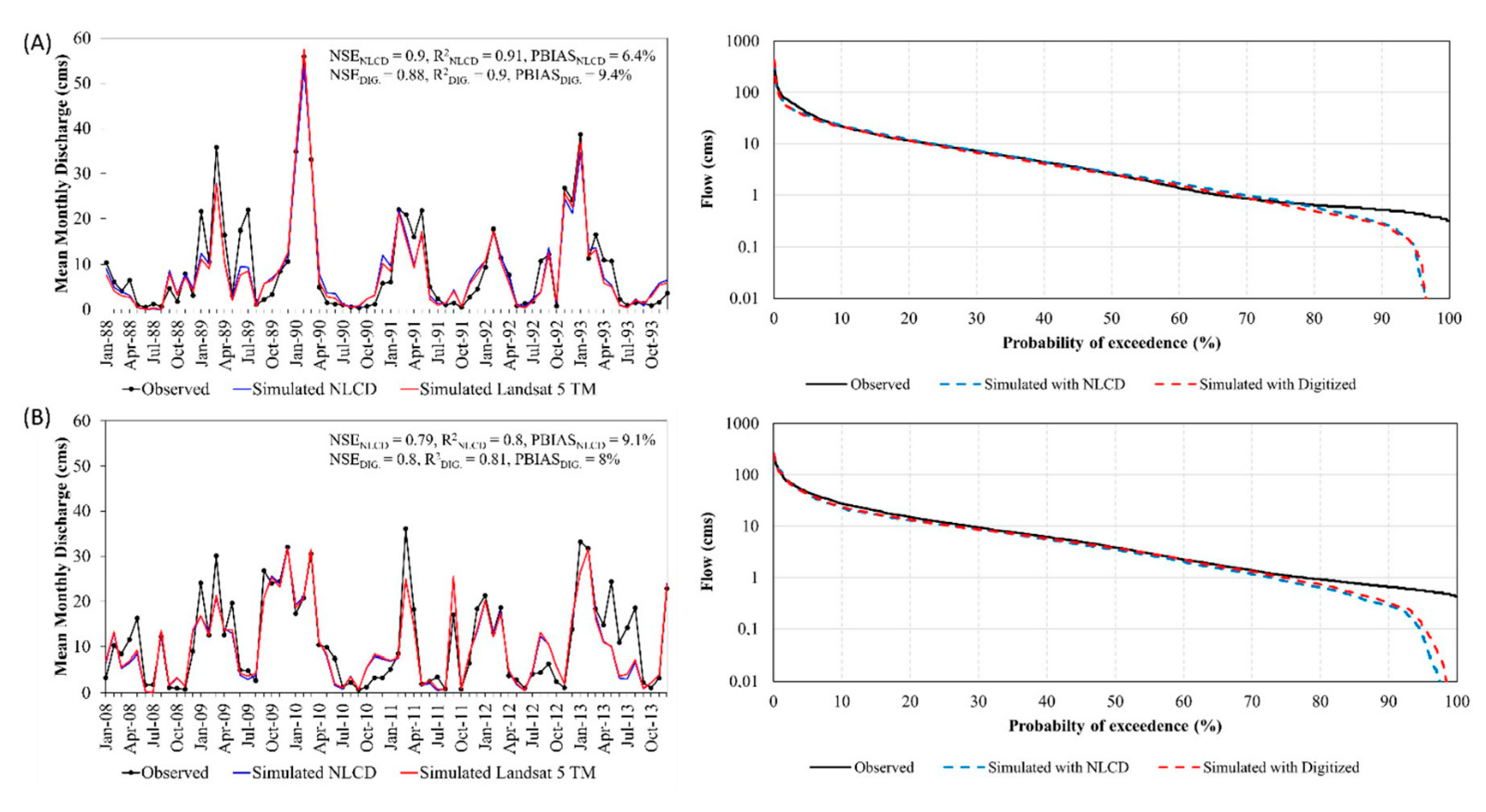
In general, there was no significant difference in simulated daily and monthly stream flows under NLCD and Digitized LULC datasets in the calibration period (Figure 3A and

Table 7. Calibration and validation results.

Daily Calibration and Validation Results—LULC Dataset	Evaluation Statistics
	R2	NSE	PBIAS (%)
Calibration (1988–1993)—NLCD LULC	0.72	0.71	6.5
Calibration (1988–1993)—Digitized LULC	0.71	0.70	9.6
Validation (2008–2013)—NLCD LULC	0.68	0.65	9.3
Validation (2008–2013)—Digitized LULC	0.70	0.67	8.2

). Simulated monthly stream flows closely matched the observed values regardless of the input LULC data. The models performed particularly well during months with high flows, and NSE and R² values higher than 0.85 were achieved, which characterizes the models’ performance in simulating monthly flows as “very good” [14]. NSE and R² values were no smaller than 0.70 at the daily time step with both LULC datasets, which can be classified as a “good” model performance [14]. Although the NSE and R² values were good, both models slightly underestimated stream flows, particularly in 1989. The overall underestimation of streamflow is supported by the PBIAS values shown in Table 7. Although the model performance is categorized as “good” in terms of PBIAS [14] using both types of LULC data, the NLCD-based model dataset had a smaller bias.

The daily flow duration curves generated by the NLCD and Digitized LULC based models look very similar (Figure 3). Both models showed good skills in matching the observed daily streamflow at the UCRW, especially the high flows (probability of exceedance ≤ 20%). On the other hand, the models performed relatively poorly in reproducing low flows (probability of exceedance ≥ 80%), showing a substantial underestimation of low flows, likely due to not including point sources in the model (point discharge data were not available).

3.2.2. SWAT Performance during the Validation Period (2008–2013)

The robustness of the calibrated models in predicting streamflow was tested under different LULC conditions than those used in the calibration period. Figure 3B compares the simulated monthly flows (time series) and daily streamflows (FDC) with observed data. Visually, the models based on 2011-NLCD and 2011-Digitized LULC yielded similar results in replicating monthly observations, with moderate underestimation, especially in months with high flows. According to the performance metrics employed, both models achieved almost identical performances in simulating monthly streamflows. Considering the statistical rating criteria developed by [14], the 2011-NLCD and 2011-Digitized models are classified as “good” predictors of monthly streamflow at the UCRW. Based on the model performance summarized in Table 7, the model based on the Digitized LULC data showed slightly better skills in predicting daily streamflow during the 2008–2013 period. Overall, both models presented good performances during validation. The performances of the 2011-NLCD and 2011-Digitized models in predicting daily streamflow can be classified as “satisfactory” based on the NSE and R² values achieved [14]. In terms of PBIAS, both models underestimated observed streamflow during validation, with slightly less underestimation under the Digitized dataset (Table 7).

The results for daily flow duration curves were very similar to the ones obtained in the calibration period, with almost no differences in NLCD and Digitized LULC based FDCs, and both models showed good skills in producing the observed daily streamflow, especially the high flows (probability of exceedance ≤ 20%). Both models did a relatively poor job predicting low flows (probability of exceedance ≥ 80%).

3.3. Influence of LULC Data on Simulated Annual and Seasonal Streamflow

The simulated mean annual stream flows throughout the entire simulation period (1988–2013) were 7.60 and 7.89 m³/s with 1992-NLCD and 1992-Digitized LULC maps, respectively. In contrast, with 2011-NLCD and 2011-Digitized LULC, they were 8.05 and 8.31 m³/s, respectively. Overall, the simulated annual streamflow was 3.6 and 3.1% higher with the 1992 and 2011 Digitized LULC datasets, respectively, compared to NLCD-based streamflow estimates.

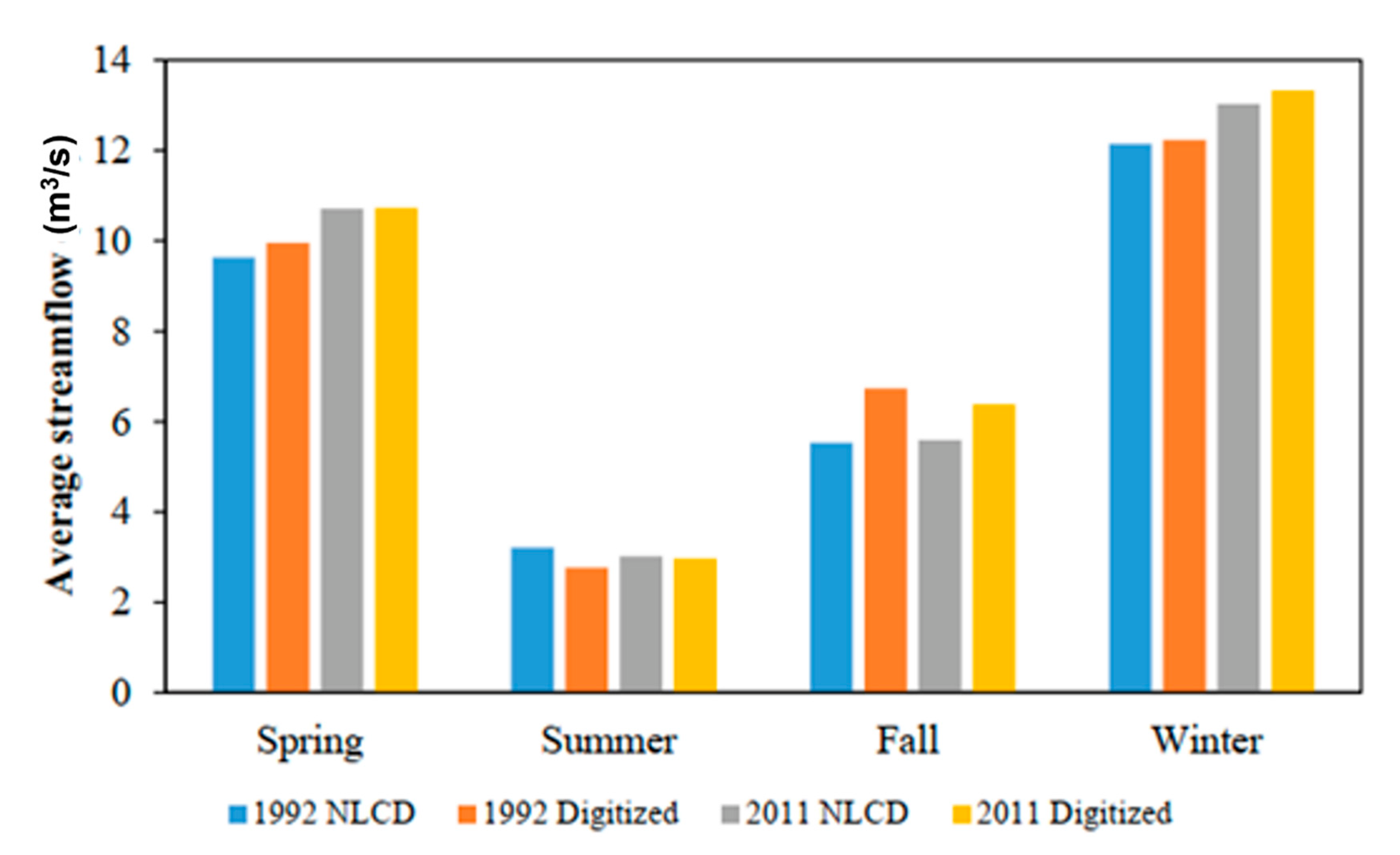
Figure 4 shows the mean seasonal stream flows simulated with the different LULC datasets. It can be seen that all LULC datasets resulted in similar model predictions of mean seasonal stream flows, although more pronounced variations were found in the fall. With the NLCD dataset, a significant increasing trend (11%) in average spring streamflow and a decreasing trend (6%) in average fall streamflow were estimated when models driven by 1992 LULC and 2011 LULC were compared. Similarly, an increasing trend was noticed during the spring (7%) and winter (9%), whereas a decreasing trend was observed during the fall (5%) using the Digitized LULC datasets. Except for the summer season, the Digitized LULC datasets consistently estimated higher stream flows at the UCRW.

3.4. Influence of LULC Data on Simulated Ecologically Relevant Flow Metrics

In the following sections, we separately discuss the impacts of LULC data for each IHA group of parameters.

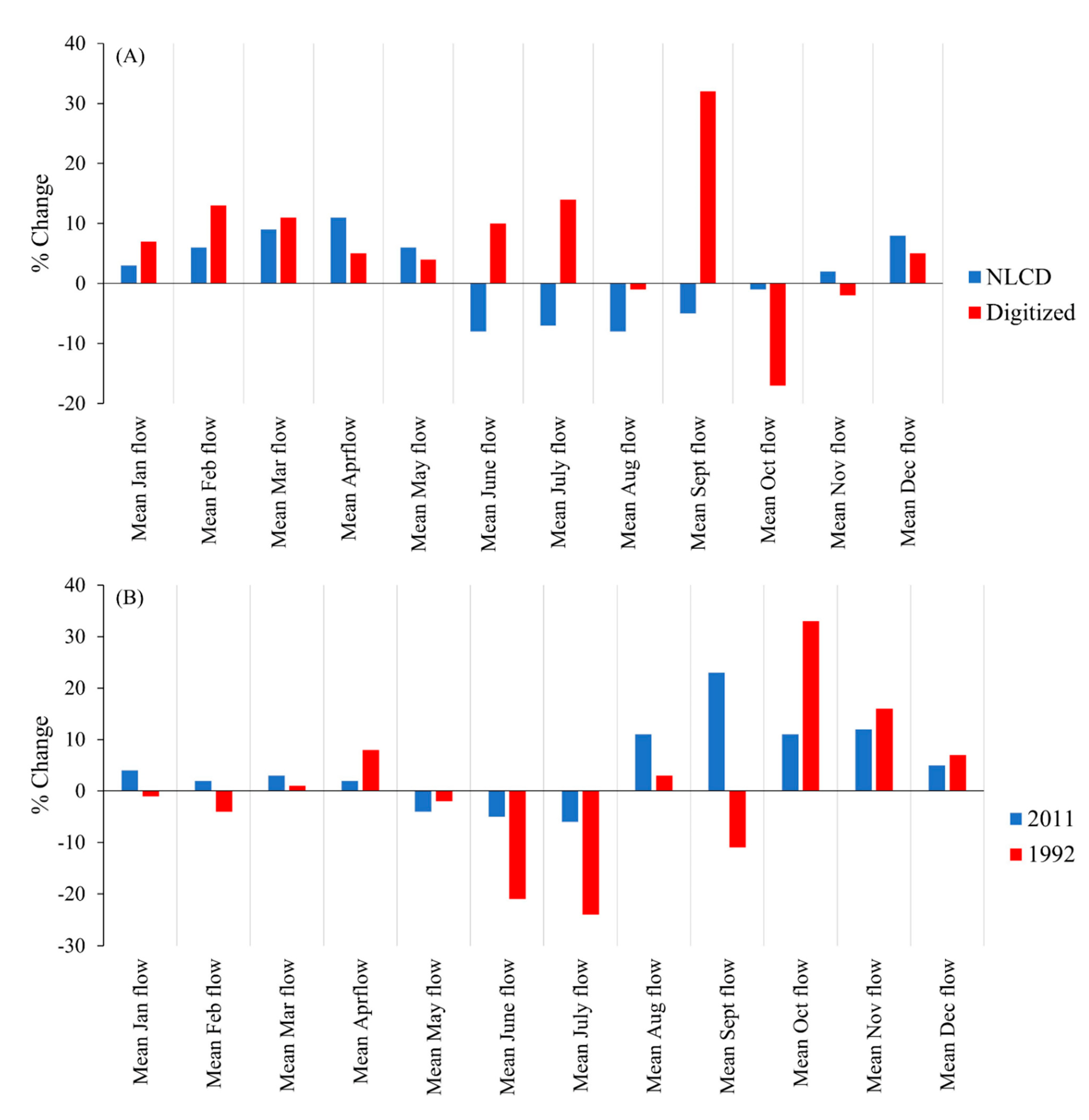
Monthly flows: Figure 5 shows the percent difference in the magnitude of monthly flows generated by different LULC sources (Equation (1)) (Figure 5A) and LULC datasets representing different years (Equation (2)) (Figure 5B). It can be seen that the percent differences were higher with the Digitized LULC inputs (especially during September–October) compared to the NLCD-based models (Figure 5A). When comparing the percent difference in monthly flows produced by the 1992 and 2011 LULC years, results showed percent differences ranging between −25% and 30% using the 1992 LULC, while the range with the 2011 datasets was −5% to 20%.

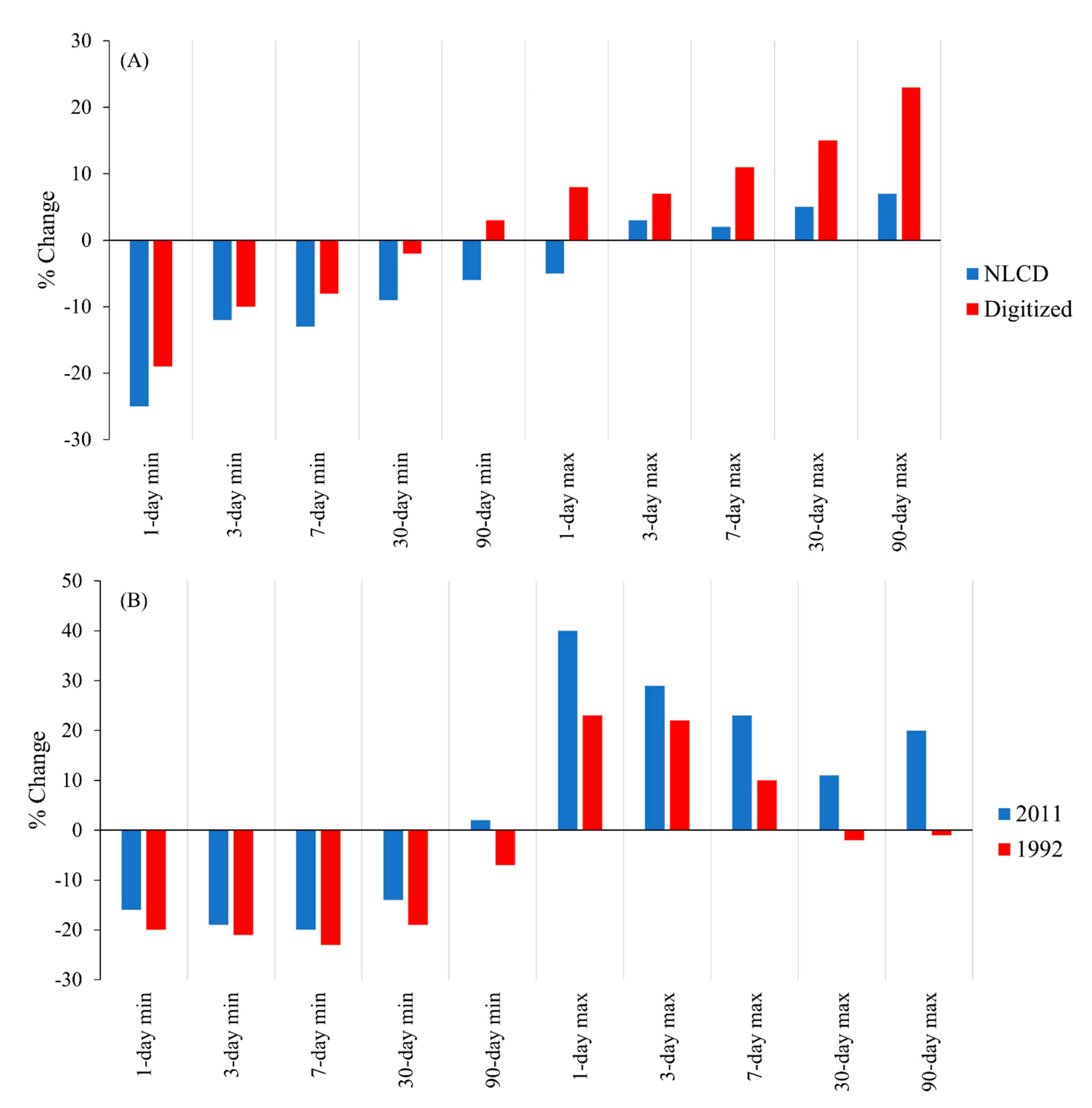
Extreme flow conditions: Figure 6 illustrates the differences in the magnitude and duration of annual extreme (min–max) flows. The 1- to 90-day minimum flows exhibited less deviation with the Digitized LULC datasets, which was particularly evident for 30- and 90-day flows (Figure 6A). On the other hand, maximum flows of different durations displayed substantially lower percent differences with the NLCD datasets. Negative percent differences in minimum flows tended to occur with 1992 and 2011, with slightly lower differences found under the 2011 LULC. Conversely, positive percent differences in maximum flows prevailed with both 1992 and 2011, with the former producing considerably smaller differences than the latter (Figure 6B).

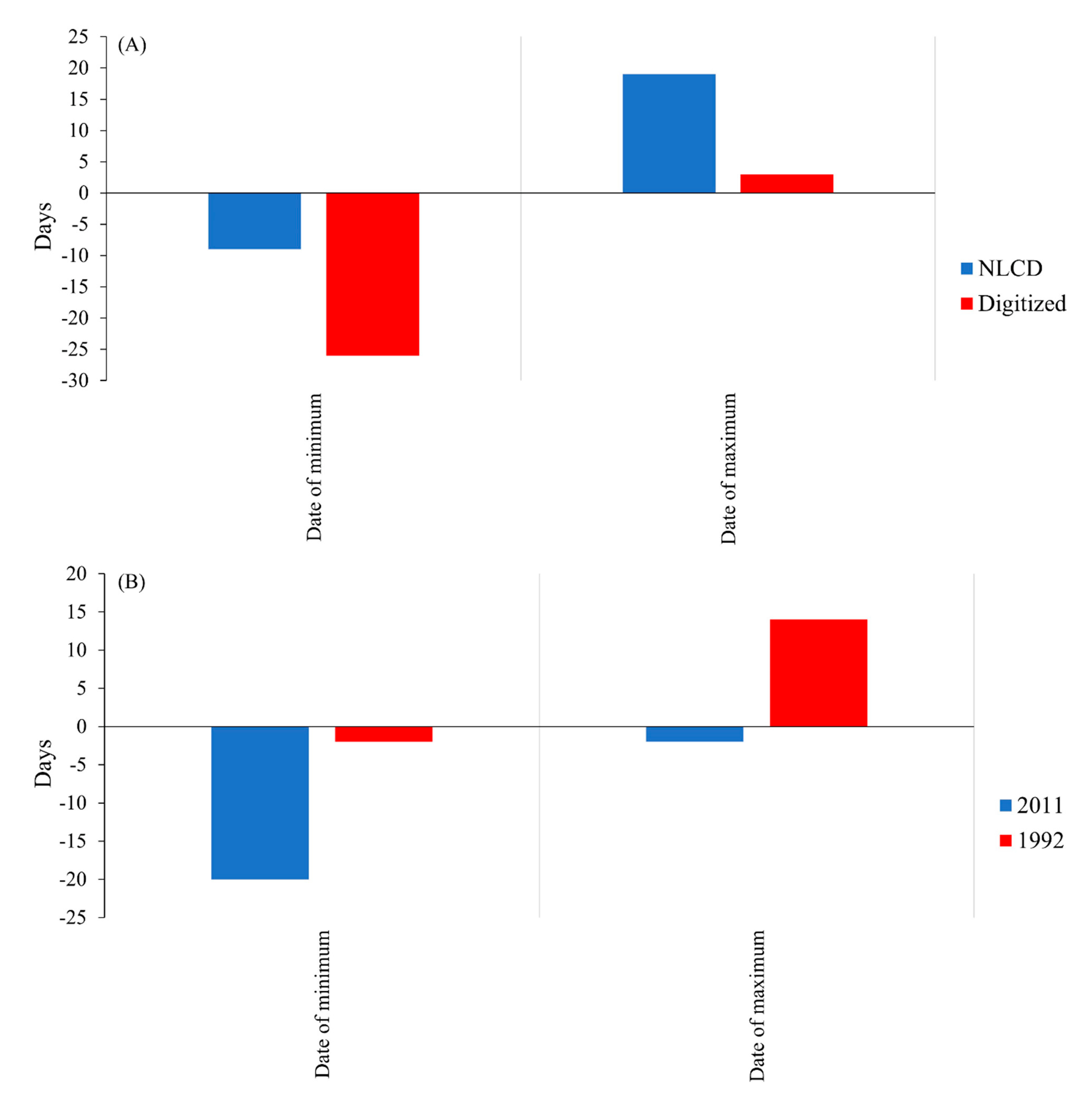
Timing of extreme flows: The differences in the predicted Julian dates of minimum and maximum flows resulting from the NLCD and Digitized LULC datasets showed an opposite trend (Figure 7A). The simulated date of 1-day minimum flow varied less with the NLCD dataset than with the Digitized data. On the other hand, the 1-day maximum flow differed by approximately three days using the Digitized datasets, whereas approximately 20 days of difference were found with the NLCD datasets. The 1992 LULC datasets led to lower differences than the 2011 LULC data in the simulated date of minimum flow. On the contrary, the 2011 datasets caused smaller changes in the predicted date of maximum flow than the 1992 LULC conditions (Figure 7B).

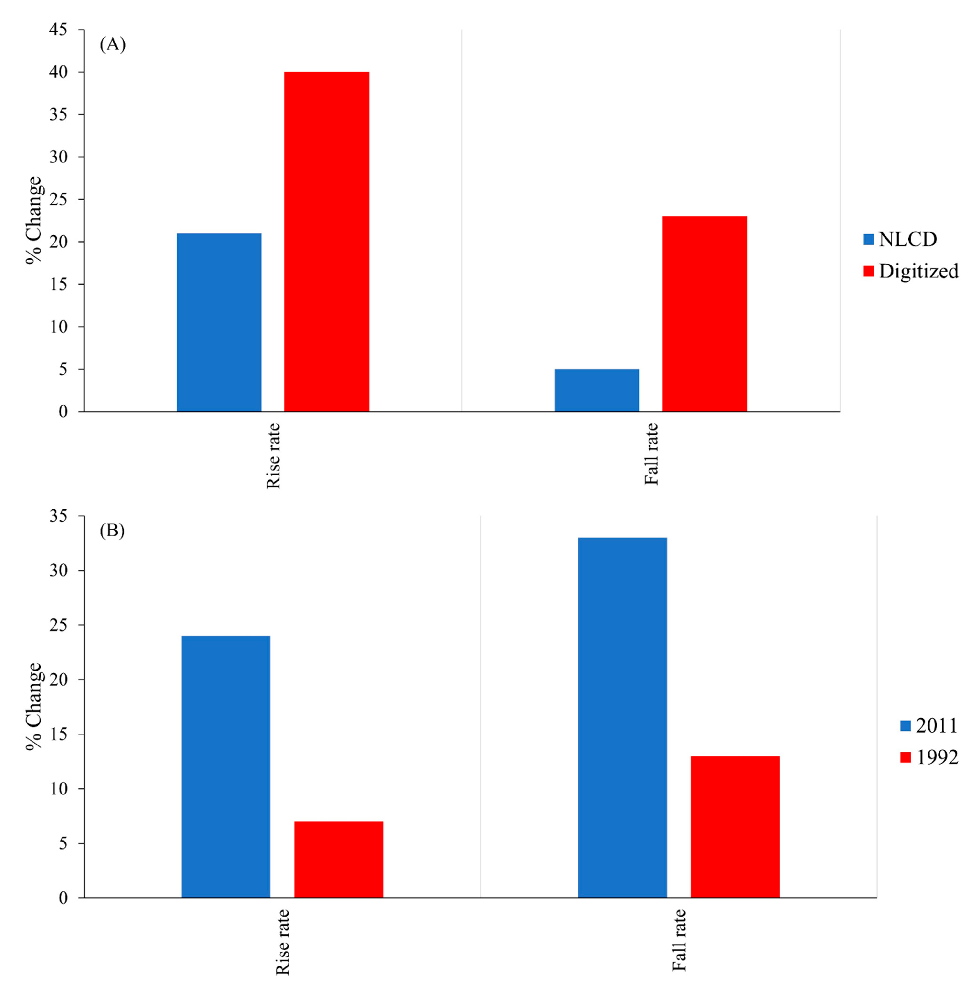
Rate of extreme flows: The NLCD datasets led to markedly lower percent differences in the simulated rise and fall rates (21 and 5% differences, respectively) compared to the Digitized LULC datasets (40 and 23% differences) (Figure 8A). The 1992 datasets led to smaller percent differences in the predicted rise and fall rates, with a deviation of 7 and 13%, respectively, as opposed to the 24 and 33% differences achieved using the 2011 LULC datasets (Figure 8B).

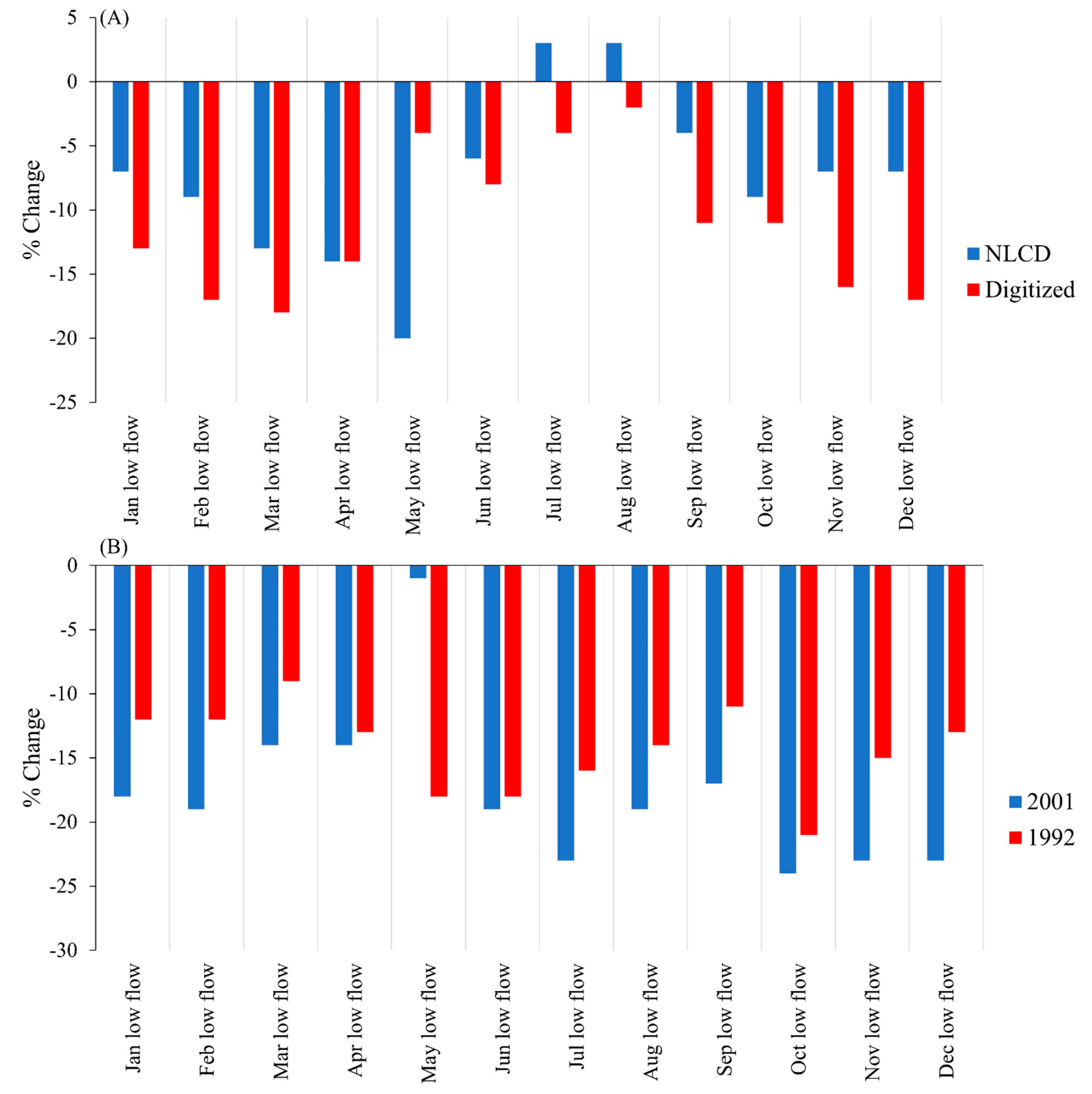
Monthly low flows: The percent changes in the magnitude of monthly low flows originating from different LULC sources and years are shown in Figure 9. In analyzing the differences in low flows stemming from different LULC sources, results indicate that the NLCD datasets produced smaller changes (except for May and August) (Figure 9A). When differences in simulated low flows under the 1992 LULC data were compared with those produced by 2011, results consistently showed smaller percent differences with the 1992 LULC data, except during May (Figure 9B), indicating a growth in uncertainty from 1992 to 2011.

4. Discussion

4.1. Influence of LULC Data on Simulated Annual and Seasonal Streamflows

According to the equifinality principle, different combinations of model parameter values may result in equally good model performances in replicating a given signal (e.g., streamflow measure at the watershed’s outlet) [9]. Model input data (e.g., LULC distribution) related to physical characteristics and spatial patterns in the watershed may influence parameter values and translate into model output uncertainties. For instance, the SWAT model handles the landscape heterogeneity by dividing the watershed into subwatersheds, which are further discretized into unique LULC, soil, and slope combinations. Thus, different LULC data translate into different watershed setups and potentially different SWAT outputs, even though other input data (e.g., climate data, soil properties, slope) are the same. While models set up based on different input data may achieve similar statistical performance and generate indistinguishable streamflow estimates, this does not guarantee similar model skills in predicting other hydrologic or water quality components (e.g., nitrate loads, evapotranspiration) [2,46,47].

In the model calibration phase of the current study, we compared SWAT’s capabilities in simulating daily streamflow during the period 1988–1993 using the NLCD LULC dataset and a Digitized dataset. Although the visual comparison of monthly hydrographs and FDCs did not show significant impacts of LULC data on streamflow predictions, the evaluation statistics indicated that the NLCD-based models yielded a slightly superior model performance at monthly and daily time steps during the calibration period (3.1% smaller bias). The apparent small influence of LULC input data on the model’s performance is most likely related to the automated model calibration process, which resulted in two different sets of parameter values yielding similar model performances, a characteristic of equifinality. This is corroborated by the fact that different LULC data sources led to changes in the parameter sensitivity rank and in the calibrated values. These results answer our first research question and support the hypothesis that models relying on different input data and varying parameter values can reach similar performances and results. It also indicates the existence of an undefined degree of equifinality associated with our models.

To answer our second research question, we tested the calibrated models in a future period where LULC changed, namely, the validation period from 2008 to 2013. This scenario presented a departure from the physical conditions of the watershed (i.e., LULC distribution and climate) for the calibration period and tested the reliability of the model in predicting streamflow under these new conditions. The similar performances obtained under the NLCD and Digitized LULC datasets confirm the equifinality of the models and suggest a low degree of variability in predicted monthly and daily streamflows regardless of the LULC dataset used.

Studies such as [15,17,18,48] have shown a relatively small influence of LULC data on model performance in simulating streamflow. Our findings are in line with these since models set up with different sources of LULC yielded similar streamflow performances under varying LULC conditions in our study. However, as discussed in the following sections, a great deal of uncertainty was found while simulating ERF parameters under different LULC sources and years.

4.2. Changes in the Temporal Evolution of Streamflow

We found minor differences in seasonal and annual stream flows, although the Digitized datasets tended to produce higher annual and seasonal streamflow rates. Annually, these differences were approximately 4%, while changes as high as 18% were found during the fall. Our findings show good agreement with those of [16], who showed less than 10% difference in annual streamflow using different sources of LULC data. The overall higher annual and seasonal streamflow generated by the Digitized LULC map compared to the NLCD product can be interpreted based on the differences in LULC detected by each dataset. Although both datasets detected similar urban fractions, the Digitized map showed substantially smaller forested areas and broader agricultural coverage. Forests are usually associated with lower water yield and runoff [49] because of the high evapotranspiration rates [50] and enhanced soil infiltration and percolation [51], while crop fields are sources of surface runoff because of soil compaction [52] and lower infiltration rates.

The LULC source exerted larger uncertainties when percent changes in the magnitude of monthly streamflow were assessed. The larger percent differences found under the Digitized datasets indicate larger LULC change from 1992 to 2011 associated with this dataset than with NLCD. Regarding the persistence in LULC uncertainties, our findings consistently show smaller uncertainties in the 2011 datasets for simulating monthly flows. We found higher discrepancies in monthly stream flows during the summer months, which may be related to the value of parameters such as CANMX and GW_REVAP. The former regulates the maximum canopy storage and influences evaporation rates in SWAT, while the latter determines the amount of water moving from the shallow aquifer to the overlying unsaturated zone. The amount of water trapped by the canopy becomes available for evaporation, which is typically higher during the summer due to increased temperatures and solar radiation rates. Similarly, the evaporation of water from the saturated zone to the unsaturated zone predominates during dry periods.

In other words, LULC datasets were found to influence the value of calibrated parameters and consequently affected the variability of simulated monthly streamflow in the UCRW. These findings are relevant since monthly flows can influence the habitat availability for aquatic organisms and properties of the water, such as temperature and dissolved oxygen levels.

4.3. Changes in Extreme Flows

Substantial differences in the magnitude of simulated maximum flows of daily, weekly, monthly, and seasonal durations were found depending on the LULC source and/or year utilized. The significantly higher percent differences found under the Digitized models indicated larger changes in LULC from 1992 to 2011 with this dataset. Considering the temporal condition of the LULC data, the 2011 datasets produced smaller percent changes in simulating minimum flows and consequently smaller uncertainties for modeling minimum flows of various durations. In contrast, smaller uncertainties in simulated maximum flows were found using the 1992 LULC datasets. The difference in forest coverage and urbanization rates in 1992 and 2011 may help interpret the differences in maximum and minimum flows simulated using the 1992 and 2011 LULC datasets. For instance, we found higher magnitudes of maximum streamflow and larger uncertainties under the 2011 LULC datasets. This is most probably related to the LULC conditions in the watershed during these periods, which consisted of fewer forests and more urban areas in 2011. The systematic underestimation/overestimation of minimum/maximum flows of various durations under different LUCL data source and temporal conditions should not come as surprise since the suite of flow metrics are computed from the same model output. In other words, if 1-day minimum flow is underestimated, for instance, it is very likely that minimum flows averaged over 7-day, 30-day, and 90-days of duration are underestimated as well. The same applies to maximum flows.

Extreme water conditions such as maximum flows of various durations may have important ecological implications since they influence the channel morphology, aquatic ecosystems, and physical habitat conditions. These ERF metrics can also impact riverine species because they influence drought stress on plants and entrapment of organisms on islands and floodplains due to rising water levels. Thus, extreme flow conditions must be investigated with caution, and uncertainties related to LULC input data should be considered when communicating the modeling results to stakeholders and/or decision-makers.

4.4. Changes in Low Flows

Low flows are extremely important for the biotic composition of aquatic and riparian ecosystems and deserve more attention in watershed modeling studies. For instance, low flows can influence the habitat of aquatic organisms, maintain suitable water temperatures and oxygen levels, provide drinking water for terrestrial animals, and affect the reproduction of fish and amphibians [23,24]. Low flows can impact the life cycle of fisheries, especially during the summer months, when the water temperature is higher [53]. Further, low flows significantly affect invertebrate communities, which are adapted to specific flow velocities and are thus extremely sensitive to fluctuations in low flows [54]. Additionally, the magnitude of low flows affects other facets of water resource management, such as infrastructure design and environmental regulation [55]. Our results suggest that different sources of LULC data can significantly affect the magnitude of simulated monthly low flows at the UCRW, which can be relevant given the importance of low flows for aquatic and riverine ecosystems. Overall, the NLCD-based models had smaller uncertainties in the magnitude of simulated monthly low flows. In other words, model runs using the 1992-NLCD and 2011-NLCD LULC datasets over the 1988–2013 period resulted in smaller percent changes in low flows compared to the 1992-Digitized and 2011-Digitized model results. This is most likely related to larger LULC change from 1992 to 2011 detected by the Digitized datasets, especially the increase in urbanized areas (Table 1). Considering the mathematical formulation of Equation (3), the negative percent differences found for both datasets (Figure 9) suggest a decreasing trend in monthly low flows at the UCRW. This finding is corroborated by studies such as [56], which have identified a decreasing trend in the magnitude of low flows across the Southeastern U.S. Further, the higher percent changes found for the 2011 LULC data imply more modeling uncertainties in predicting low flows with these datasets than with the 1992 LULC maps. This may be due to the urbanization from 1992 to 2011, which increased the impervious cover.

5. Conclusions

The results presented here indicate that different sources and years of LULC input data can yield similar performances in watershed models based on statistical rating metrics such as NSE, R², and PBIAS, yet marked differences were found in analyzing other simulated flow metrics. This suggests that traditionally used model evaluation criteria (hard data approach) may not be appropriate when the goal of the model application goes beyond streamflow prediction at the watershed outlet. We assessed the uncertainty in simulated ecological flow parameters (soft data approach) attributable to different sources of LULC information. Results consistently showed smaller uncertainties in predicting ERF parameters when using the NLCD datasets. The Digitized data only yielded smaller uncertainties in predicting minimum flows of various durations and the Julian date of 1-day maximum flow. Therefore, it can be concluded that incorporation of soft data during modeling processes has a positive impact over the quality of simulation results.

We also assessed whether uncertainties stemming from LULC sources persisted from 1992 to 2011. Our findings suggest that uncertainties from LULC vary according to the ERF metric analyzed. For example, the 1992 LULC datasets produced smaller uncertainties in simulated low flows and maximum flows of various durations. Additionally, the 1992 LULC data led to smaller uncertainties in simulating the date of minimum flows of 1-day duration, as well as the rise and fall rates. On the other hand, smaller uncertainties in the magnitude of simulated monthly flows and the date of maximum flow were found under the 2011 LULC conditions.

The UCRW is known for its aquatic biodiversity, aesthetic beauty, and unique landscape features. However, this watershed has undergone rapid urbanization since the 1990s, which has affected the watershed flow regimes. Such alterations in the flow regime can significantly impact the aquatic and riparian biota and threaten the watershed’s biodiversity. For instance, the Cahaba lilies (Hymenocallis coronaria) have been wiped out from many areas within the watershed due to flow fluctuations. Thus, the consequences of LULC changes on water resources and their ramifications for riverine ecosystems should be investigated carefully. As a standard input to most watershed-scale models, LULC distribution must be accurately captured in watershed modeling efforts to achieve reliable model predictions capable of supporting decision-making. The results of our study can be beneficial for local stakeholders and decision-makers in developing science-based management and development plans for sustainable water use and LULC changes in the UCRW. The methodology presented in the current study is relatively simple and can be easily replicated in other watershed systems or further scrutinized in the UCRW.

References

- Triana, J.S.A.; Chu, M.L.; Guzman, J.A.; Moriasi, D.N.; Steiner, J.L. Beyond model metrics: The perils of calibrating hydrologic models. J. Hydrol. 2019, 578, 124032. [Google Scholar] [CrossRef]
- Yen, H.; Bailey, R.T.; Arabi, M.; Ahmadi, M.; White, M.J.; Arnold, J.G. The Role of Interior Watershed Processes in Improving Parameter Estimation and Performance of Watershed Models. J. Environ. Qual. 2014, 43, 1601. [Google Scholar] [CrossRef] [PubMed]
- Feng, D.; Beighley, E. Identifying uncertainties in hydrologic fluxes and seasonality from hydrologic model components for climate change impact assessments. Hydrol. Earth Syst. Sci. 2020, 24, 2253–2267. [Google Scholar] [CrossRef]
- Breuer, L.; Huisman, J.A.; Frede, H.-G. Monte Carlo assessment of uncertainty in the simulated hydrological response to land use change. Environ. Model. Assess. 2006, 11, 209–218. [Google Scholar] [CrossRef]
- Pai, N.; Saraswat, D. Impact of Land Use and Land Cover Categorical Uncertainty on SWAT Hydrologic Modeling. Trans. ASABE 2013, 56, 1387–1397. [Google Scholar] [CrossRef]
- Yen, H.; Wang, X.; Fontane, D.G.; Harmel, R.D.; Arabi, M. A framework for propagation of uncertainty contributed by parameterization, input data, model structure, and calibration/validation data in watershed modeling. Environ. Model. Softw. 2014, 54, 211–221. [Google Scholar] [CrossRef]
- Eckhardt, K.; Breuer, L.; Frede, H.-G. Parameter uncertainty and the significance of simulated land use change effects. J. Hydrol. 2003, 273, 164–176. [Google Scholar] [CrossRef]
- Niraula, R.; Meixner, T.; Norman, L.M. Determining the importance of model calibration for forecasting absolute/relative changes in streamflow from LULC and climate changes. J. Hydrol. 2015, 522, 439–451. [Google Scholar] [CrossRef]
- Beven, K.; Freer, J. Equifinality, data assimilation, and uncertainty estimation in mechanistic modelling of complex environmental systems using the GLUE methodology. J. Hydrol. 2001, 249, 11–29. [Google Scholar] [CrossRef]
- Her, Y.; Chaubey, I. Impact of the numbers of observations and calibration parameters on equifinality, model performance, and output and parameter uncertainty. Hydrol. Process. 2015, 29, 4220–4237. [Google Scholar] [CrossRef]
- Kamali, B.; Abbaspour, K.C.; Yang, H. Assessing the Uncertainty of Multiple Input Datasets in the Prediction of Water Resource Components. Water 2017, 9, 709. [Google Scholar] [CrossRef] [Green Version]
- Beven, K. Towards integrated environmental models of everywhere: Uncertainty, data and modelling as a learning process. Hydrol. Earth Syst. Sci. 2007, 11, 460–467. [Google Scholar] [CrossRef]
- Moriasi, D.N.; Arnold, J.G.; Van Liew, M.W.; Bingner, R.L.; Harmel, R.D.; Veith, T.L. Model Evaluation Guidelines for Systematic Quantification of Accuracy in Watershed Simulations. Trans. ASABE 2007, 50, 885–900. [Google Scholar] [CrossRef]
- Moriasi, D.N.; Gitau, M.W.; Pai, N.; Daggupati, P. Hydrologic and water quality models: Performance measures and evaluation criteria. Am. Soc. Agric. Biol. Eng. 2015, 58, 1763–1785. [Google Scholar]
- El-Sadek, A.; Irvem, A. Evaluating the impact of land use uncertainty on the simulated streamflow and sediment yield of the Seyhan River basin using the SWAT model. Turk. J. Agric. For. 2014, 38, 515–530. [Google Scholar] [CrossRef]
- Chen, P.; Luzio, M.D.; Arnold, J.G. Impact of Two Land-Cover Data Sets on Stream Flow and Total Nitrogen Simulations using a Spatially Distributed Hydrologic Model. In Proceedings of the Global Priorities in Land Remote Sensing, Sioux Falls, SD, USA, 23–27 October 2005; Available online: https://www.semanticscholar.org/paper/IMPACT-OF-TWO-LAND-COVER-DATA-SETS-ON-STREAM-FLOW-A-Chen-Arnold/4261153b5661fb33212b54bfa721e57e79273408 (accessed on 15 October 2021).
- Wang, Q.; Liu, R.; Men, C.; Guo, L.; Miao, Y. Effects of dynamic land use inputs on improvement of SWAT model performance and uncertainty analysis of outputs. J. Hydrol. 2018, 563, 874–886. [Google Scholar] [CrossRef]
- Yen, H.; Sharifi, A.; Kalin, L.; Mirhosseini, G.; Arnold, J.G. Assessment of model predictions and parameter transferability by alternative land use data on watershed modeling. J. Hydrol. 2015, 527, 458–470. [Google Scholar] [CrossRef]
- Cotter, A.S.; Chaubey, I.; Costello, T.A.; Soerens, T.S.; Nelson, M.A. Water quality model output uncertainty as affected by spatial resolution of input data. JAWRA J. Am. Water Resour. Assoc. 2003, 39, 977–986. [Google Scholar] [CrossRef]
- Huang, J.; Zhou, P.; Zhou, Z.; Huang, Y. Assessing the Influence of Land Use and Land Cover Datasets with Different Points in Time and Levels of Detail on Watershed Modeling in the North River Watershed, China. Int. J. Environ. Res. Public Health 2013, 10, 144–157. [Google Scholar] [CrossRef]
- Yen, H.; White, M.J.; Arnold, J.G.; Keitzer, S.C.; Johnson, M.-V.V.; Atwood, J.D.; Daggupati, P.; Herbert, M.E.; Sowa, S.P.; Ludsin, S.A.; et al. Western Lake Erie Basin: Soft-data-constrained, NHDPlus resolution watershed modeling and exploration of applicable conservation scenarios. Sci. Total Environ. 2016, 569–570, 1265–1281. [Google Scholar] [CrossRef] [Green Version]
- Pérez-Sánchez, J.; Senent-Aparicio, J.; Santa-María, C.M.M.; López-Ballesteros, A. Assessment of Ecological and Hydro-Geomorphological Alterations under Climate Change Using SWAT and IAHRIS in the Eo River in Northern Spain. Water 2020, 12, 1745. [Google Scholar] [CrossRef]
- Richter, B.D.; Baumgartner, J.V.; Powell, J.; Braun, D.P. A Method for Assessing Hydrologic Alteration within Ecosystems. Conserv. Biol. 1996, 10, 1163–1174. [Google Scholar] [CrossRef] [Green Version]
- Poff, N.L.; Allan, J.D.; Bain, M.B.; Karr, J.R.; Prestegaard, K.L.; Richter, B.D.; Sparks, R.E.; Stromberg, J.C. The Natural Flow Regime. Biosciemce 1997, 47, 769–784. [Google Scholar] [CrossRef]
- Wu, N.; Qu, Y.; Guse, B.; Makarevičiūtė, K.; To, S.; Riis, T.; Fohrer, N. Hydrological and environmental variables outperform spatial factors in structuring species, trait composition, and beta diversity of pelagic algae. Ecol. Evol. 2018, 8, 2947–2961. [Google Scholar] [CrossRef] [PubMed]
- Kiesel, J.; Kakouei, K.; Guse, B.; Fohrer, N.; Jähnig, S.C. When is a hydrological model sufficiently calibrated to depict flow preferences of riverine species? Ecohydrology 2020, 13, e2193. [Google Scholar] [CrossRef] [Green Version]
- Arnold, J.G.; Srinivasan, R.; Muttiah, R.S.; Williams, J.R. Large Area Hydrologic Modeling and Assessment Part I: Model Development. JAWRA J. Am. Water Resour. Assoc. 1998, 34, 73–89. [Google Scholar] [CrossRef]
- The Nature Conservancy. Indicators of Hydrologic Alteration Version 7.1 User’s Manual. 2009. Available online: https://www.conservationgateway.org/Documents/IHAV7.pdf (accessed on 9 January 2020).
- Montiel, D.; Lamore, A.F.; Stewart, J.; Lambert, W.J.; Honeck, J.; Lu, Y.; Warren, O.; Adyasari, D.; Moosdorf, N.; Dimova, N. Natural groundwater nutrient fluxes exceed anthropogenic inputs in an ecologically impacted estuary: Lessons learned from Mobile Bay, Alabama. Biogeochemistry 2019, 145, 1–33. [Google Scholar] [CrossRef]
- Dosdogru, F.; Kalin, L.; Wang, R.; Yen, H. Potential impacts of land use/cover and climate changes on ecologically relevant flows. J. Hydrol. 2020, 584, 124654. [Google Scholar] [CrossRef]
- Onorato, D.; Angus, R.A.; Marion, K.R. Historical Changes in the Ichthyofaunal Assemblages of the Upper Cahaba River in Alabama Associated with Extensive Urban Development in the Watershed. J. Freshw. Ecol. 2000, 15, 47–63. [Google Scholar] [CrossRef] [Green Version]
- Onorato, D.; Marion, K.R.; Angus, R.A. Longitudinal Variations in the Ichthyofaunal Assemblages of the Upper Cahaba River: Possible Effects of Urbanization in a Watershed. J. Freshw. Ecol. 1998, 13, 139–154. [Google Scholar] [CrossRef] [Green Version]
- Morse, K.J. The Effects of Urbanization on the Health of Fish and Benthic Macroinvertebrate Communities in the Upper Cahaba River Watershed. Ph.D. Thesis, The University of Alabama at Birmingham, Birmingham, AL, USA, 2005. [Google Scholar]
- Gassman, P.W.; Reyes, M.R.; Green, C.H.; Arnold, J.G. The Soil and Water Assessment Tool: Historical Development, Applications, and Future Research Directions. Trans. ASABE 2007, 50, 1211–1250. [Google Scholar] [CrossRef] [Green Version]
- Gassman, P.W.; Sadeghi, A.M.; Srinivasan, R. Applications of the SWAT Model Special Section: Overview and Insights. J. Environ. Qual. 2014, 43, 1–8. [Google Scholar] [CrossRef]
- Neitsch, S.L.; Arnold, J.G.; Kiniry, J.R.; Williams, J.R. Soil and Water Assessment Tool Theoretical Documentation: Version 2009; Texas Water Resources Institute Technical Report No. 406; Texas Water Resources Institute: College Station, TX, USA, 2011. [Google Scholar]
- Abbaspour, K.C.; Vaghefi, S.A.; Yang, H.; Srinivasan, R. Global soil, landuse, evapotranspiration, historical and future weather databases for SWAT Applications. Sci. Data 2019, 6, 263. [Google Scholar] [CrossRef] [Green Version]
- Cunge, J.A. On The Subject of a Flood Propagation Computation Method (Musklngum Method). J. Hydraul. Res. 1969, 7, 205–230. [Google Scholar] [CrossRef]
- Winchell, M.; Srinivasan, R.; Di Luzio, M.; Bosch, J.M. ArcSWAT Interface for SWAT 2005. User’s Guide; Blackland Research Center, Texas Agricultural Experiment Station: Temple, TX, USA, 2009. [Google Scholar]
- Abbaspour, K.C. SWAT Calibration and Uncertainty Programs: Eawag Aquatic Research; Eawag, Swiss Federal Institute of Aquatic Science and Technology: Dubendorf, Switzerland, 2015; p. 100. [Google Scholar]
- Eckhardt, K.; Arnold, J. Automatic calibration of a distributed catchment model. J. Hydrol. 2001, 251, 103–109. [Google Scholar] [CrossRef]
- Krause, P.; Boyle, D.P.; Bäse, F. Comparison of different efficiency criteria for hydrological model assessment. Adv. Geosci. 2005, 5, 89–97. [Google Scholar] [CrossRef] [Green Version]
- Gillespie, B.R.; Desmet, S.; Kay, P.; Tillotson, M.; Brown, L. A critical analysis of regulated river ecosystem responses to managed environmental flows from reservoirs. Freshw. Biol. 2015, 60, 410–425. [Google Scholar] [CrossRef]
- Hu, W.-W.; Wang, G.; Deng, W.; Li, S.-N. The influence of dams on ecohydrological conditions in the Huaihe River basin, China. Ecol. Eng. 2008, 33, 233–241. [Google Scholar] [CrossRef]
- Mezger, G.; del Tánago, M.G.; De Stefano, L. Environmental flows and the mitigation of hydrological alteration downstream from dams: The Spanish case. J. Hydrol. 2020, 598, 125732. [Google Scholar] [CrossRef]
- Kiesel, J.; Guse, B.; Pfannerstill, M.; Kakouei, K.; Jähnig, S.C.; Fohrer, N. Improving hydrological model optimization for riverine species. Ecol. Indic. 2017, 80, 376–385. [Google Scholar] [CrossRef]
- Shrestha, R.R.; Peters, D.L.; Schnorbus, M.A. Evaluating the ability of a hydrologic model to replicate hydro-ecologically relevant indicators. Hydrol. Process. 2014, 28, 4294–4310. [Google Scholar] [CrossRef]
- Di Luzio, M.; Leh, M.D.; Cothren, J.D.; Van Brahana, J.; Asante, K. Effects of land-use land-cover data resolution and classification methods on SWAT model flow predictive reliability. Int. J. Hydrol. Sci. Technol. 2017, 7, 39. [Google Scholar] [CrossRef]
- Sun, G.; McNulty, S.; Lu, J.; Amatya, D.; Liang, Y.; Kolka, R. Regional annual water yield from forest lands and its response to potential deforestation across the southeastern United States. J. Hydrol. 2005, 308, 258–268. [Google Scholar] [CrossRef]
- McLaughlin, D.L.; Kaplan, D.A.; Cohen, M.J. Managing Forests for Increased Regional Water Yield in the Southeastern U.S. Coastal Plain. JAWRA J. Am. Water Resour. Assoc. 2013, 49, 953–965. [Google Scholar] [CrossRef]
- Kim, Y.; Band, L.E.; Song, C. The Influence of Forest Regrowth on the Stream Discharge in the North Carolina Piedmont Watersheds. JAWRA J. Am. Water Resour. Assoc. 2014, 50, 57–73. [Google Scholar] [CrossRef]
- Alaoui, A.; Rogger, M.; Peth, S.; Blöschl, G. Does soil compaction increase floods? A review. J. Hydrol. 2018, 557, 631–642. [Google Scholar] [CrossRef]
- Burn, D.H.; Buttle, J.M.; Caissie, D.; MacCulloch, G.; Spence, C.; Stahl, K. The Processes, Patterns and Impacts of Low Flows Across Canada. Can. Water Resour. J. Rev. Can. Ressour. Hydr. 2008, 33, 107–124. [Google Scholar] [CrossRef] [Green Version]
- Suren, A.M.; Jowett, I.G. Effects of floods versus low flows on invertebrates in a New Zealand gravel-bed river. Freshw. Biol. 2006, 51, 2207–2227. [Google Scholar] [CrossRef]
- Stephens, T.A.; Bledsoe, B.P. Low-Flow Trends at Southeast United States Streamflow Gauges. J. Water Resour. Plan. Manag. 2020, 146, 04020032. [Google Scholar] [CrossRef]
- Sadri, S.; Kam, J.; Sheffield, J. Nonstationarity of low flows and their timing in the eastern United States. Hydrol. Earth Syst. Sci. 2016, 20, 633–649. [Google Scholar] [CrossRef] [Green Version]
Figure 1.
Location of the Upper Cahaba River watershed.
Figure 2.
LULC datasets used in this study. (TM: Thematic Mapper; NLCD: National Land Cover Database).
Figure 3.
Observed and simulated mean monthly streamflows and daily flow duration curves during the (A) calibration and (B) validation periods.
Figure 4.
Comparison of seasonal streamflow.
Figure 5.
Changes in monthly streamflow. Percent differences in the magnitude of monthly streamflow due to the source of LULC data (A) and due to the temporal condition of LULC distribution in the watershed using 1992 and 2011 LULC data (B).
Figure 6.
Changes in annual extreme water conditions. Percent differences in the magnitude of extreme water conditions due to the source of LULC data (A) and due to the temporal condition of LULC distribution in the watershed using 1992 and 2011 LULC data (B).
Figure 7.
Changes in the timing of annual extreme flows due to the source of LULC data (A) and due to the temporal condition of LULC distribution in the watershed using 1992 and 2011 LULC data (B).
Figure 8.
Changes in the rate and frequency of streamflow. Percent differences in the rise and fall rates due to the source of LULC data (A) and due to the temporal condition of LULC distribution in the watershed using 1992 and 2011 LULC data (B).
Figure 9.
Changes in monthly low flows. Percent differences in the magnitude of monthly low flows due to the source of LULC data (A) and due to the temporal condition of LULC distribution in the watershed using 1992 and 2011 LULC data (B).