Identification of Hydraulic Parameters Influencing the Hydraulic Erodibility of Spillway Flow Channels

Abstract

The rock mass erosion of dam spillways, a phenomenon involving the interaction between the hydraulic load of water and the capability of the rock mass to resist its destruction, remains a critical safety issue. The erosion resistance of a rock mass can be estimated through several erodibility indices, including those of Kirsten, Pells or Bollaert. Several indices have been developed to link rock resistance to the hydraulic parameters of water, i.e., the hydraulic load applied on a rock mass. The developed indices use the average flow velocity, the average shear stress on the bottom of the flow channel, the stress applied to the internal joints of fractured rock mass, the dynamic impulse force, and the power dissipation of water to represent the erosive force of water. From these indices, several methods of assessing hydraulic erosion have been developed, and all use the threshold line concept. Nonetheless, several uncertainties are associated with these methods. This paper presents and discusses the various means of calculating the erosive force of water as a hazard parameter for predicting potential rock erosion. The representativeness of these approaches is also discussed, and we clarify nuances associated with each method. We then provide guidelines for future research aimed at improving estimates of the erosive force of the water within spillway flow channels.

1. Introduction

The notion of the hydraulic erodibility of a rock mass emerged around 1900 after observations of the degradation of rock masses under bridges [1]. Several cases of erosion downstream of dam spillways have since been observed, for example, the Tarbela dam in Pakistan in 1976 [2] and the Kariba dam in Zambia in 1962 [3]. Much research has focused on understanding this phenomenon, and several methods have been developed for evaluating the hydraulic erodibility of a rock mass using semi-empirical and semi-analytical methods. These methods have applied the concept of the “threshold line,” [4,5] a correlation between a hydraulic hazard parameter (e.g., shear stress, hydraulic power, and hydraulic energy) and the capacity of the rock to resist destruction. This concept is based on three erosion mechanisms in particular: dynamic block removal, brittle fracturing, and the continuous fragile fracturing of the rock mass [6,7,8]. Turbulent flow is the flow mode that can produce these different erosion mechanisms.

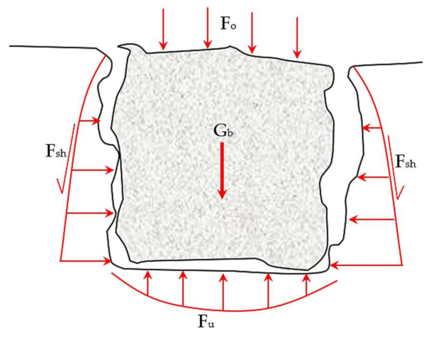
Erosion by the removal of blocks is a process that depends on the water pressure within the joints of the fractured rock mass. The amplitude of the fluctuating pressure changes with time during a turbulent flow, and the pressure applied inside the rock joints can increase pressure directly below the blocks. Moreover, the rock mass is eroded by the dynamic expulsion of the blocks when the lifting pressure under the block exceeds the resistance force of the block in the rock mass (Figure 1). The parameters affecting the resistance of the block are the submerged weight of the block $\left(G_b\right)$, the pressure on top of the block $(F_o)$, and the shear resistance along the sides of the block $(F_{sh})$.

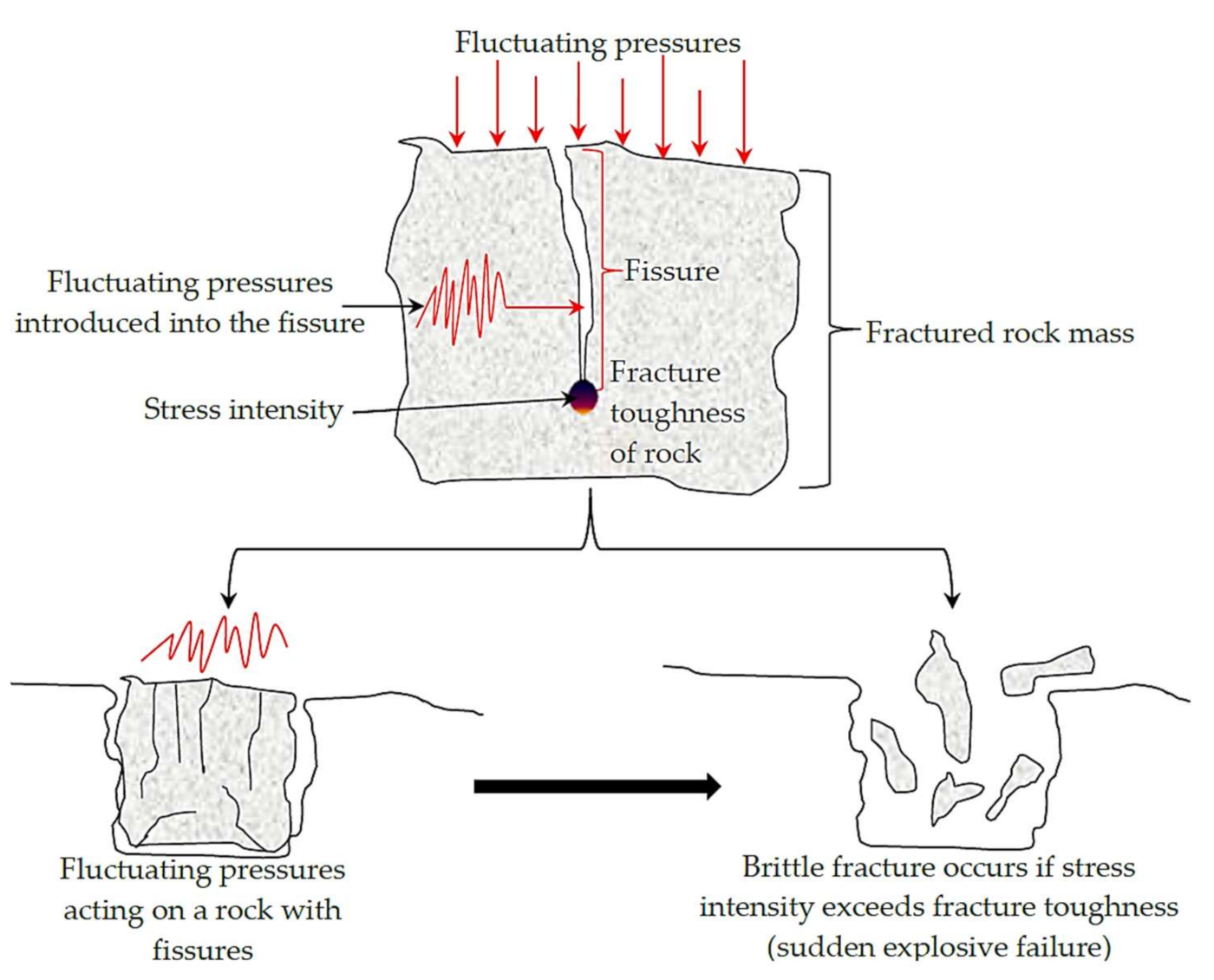
The second mechanism enabling the erosion of a rock mass is brittle fracturing or instant hydrofracturing. This mechanism occurs when the intensity of the fluctuating pressure-induced stress in the joints is greater than the resistance of the rock, and, hence, the rock mass breaks into small pieces owing to fragile failure (Figure 2).

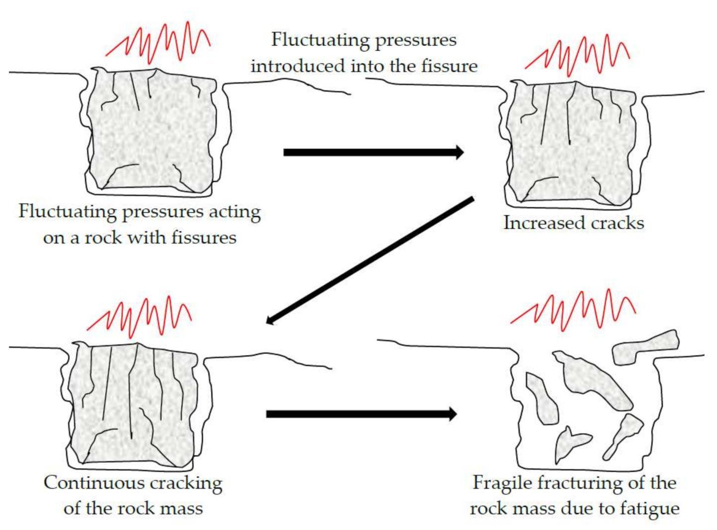
The final mechanism of erosion is continuous fragile fracturing or fatigue erosion. This mechanism occurs when the instantaneous brittle fracture of rock mass is not possible, as the intensity of the stress in the joints does not exceed the resistance of the rock mass. The rock mass is eroded, however, by fatigue pressure loads that exist in the joints. This type of erosion is highly dependent on time (Figure 3).

From these three erosion mechanisms, various indices have been developed to represent the resistance of a rock mass. These indices include the Kirsten index$\left(K_h\right)$, Bollaert’s in situ resistance of a rock mass $(K_{I,in}$), and the indices of Pells, which are the geological strength index for erodibility $\left(eGSI\right)$ and the rock mass erodibility index $(RMEI$). The hydraulic hazard parameter of water has been mainly represented by the dissipation of energy rate$({\Pi }_{UD} in {\mathrm{kW} \mathrm{m}}^{-2}$), although other parameters have been used. For example, Bollaert et al. [6] estimated the hydraulic hazard parameter of water in terms of the stress applied in a joint present within a rock mass$(K_I in {\mathrm{MPa} \mathrm{m}}^{1/2})$ and in the form of force dynamic impulse or block lifting force$(I_{impuls} in {\mathrm{Kg} \mathrm{m} \mathrm{s}}^{-1})$. Pells et al. [9] illustrated that the average flow velocity $\left(\overline{u} in {\mathrm{m} \mathrm{s}}^{-1}\right)$ and the average shear stress on the bottom surface of flow channel $\left({\overline{\tau }}_b in \mathrm{Pa}\right)$ are suitable indicators for representing the hydraulic erosion hazard for a fractured rock mass. Among these above-listed parameters, energy dissipation was selected by Bieniawski [10], Moore [11], Annandale [4,12], Kirsten [13], and Pells [5] (among others) to estimate the hydraulic hazard parameter of different possible flow conditions in spillways. Annandale [4] maintained that the dissipation of hydraulic power $\left({\Pi }_{UD}\right)$ provides a good approximation of turbulent fluctuations. Moreover, a large combination of spillway geometry and flow types can be associated with a given measure of ${\Pi }_{UD}$. Because the determination of ${\Pi }_{UD}$ is relatively easy to perform, this also greatly favors the use of ${\Pi }_{UD}$.

Although the resistance indices of the rock mass and the hydraulic power indices have been commonly used to evaluate the hydraulic erodibility, these methods have produced inconsistencies in some cases. These inconsistencies likely stem from two sources: the estimation of erosive force and the uncertainty linked to the indices for defining the resistance of a fractured rock mass. Previously, Boumaiza et al. [14] evaluated the weaknesses of the resistance of rock mass indices for the hydraulic erosion process. Here, we review the indices of the erosive force to determine whether erodibility assessment methods are also influenced by these hydraulic power indices and therefore represent (or not) a source of the produced inconsistencies in assessments of the hydraulic erodibility of a rock mass. Because of the large number of proposed indices, we review the various estimation methods of indices developed to represent the erosive force of water (waterpower) for various spillway flow modes. We highlight the advantages and disadvantages of each index and discuss the representativeness of each. We suggest that these indices do not effectively represent the erosive force of the water; we therefore offer potential research avenues to develop a better characterization of the erosive force of water.

In the following sections, we summarize the types of spillways and their operating mode. The different methods for estimating the hydraulic hazard parameters for rock mass erosion are then presented, including the estimation of the average shear stress at the bottom surface of a flow channel, the average flow velocity in open channels, the applied stresses inside joints, the block lifting force, and the dissipation of power or energy from a flow channel. We also discuss the limitations of these methods.

2. Types of Spillways and Their Operating Mode

The overflow structures in dams can be divided into two categories on the basis of their frequency of use: spillways (fuse-plug or emergency spillways) and regulation structures (service or auxiliary spillways). A spillway returns the excess water arriving at the dam during periods of flooding to the river. The return period of flooding determines the frequency of this occasional use. In contrast, regulation structures manage the flow rate, ensuring a relatively continuous transfer of water to the river. Despite the significant operational differences between the two structures, their designs and configurations are similar. Structures in each category vary in their specific configurations depending on site topography and geology. These on-site properties determine the types of spillway that are installed, for example [15]:

• ogee spillway,
• chute spillway,
• side-channel spillway,
• shaft or tunnel spillway,
• siphon spillway,
• and free over-fall spillway.

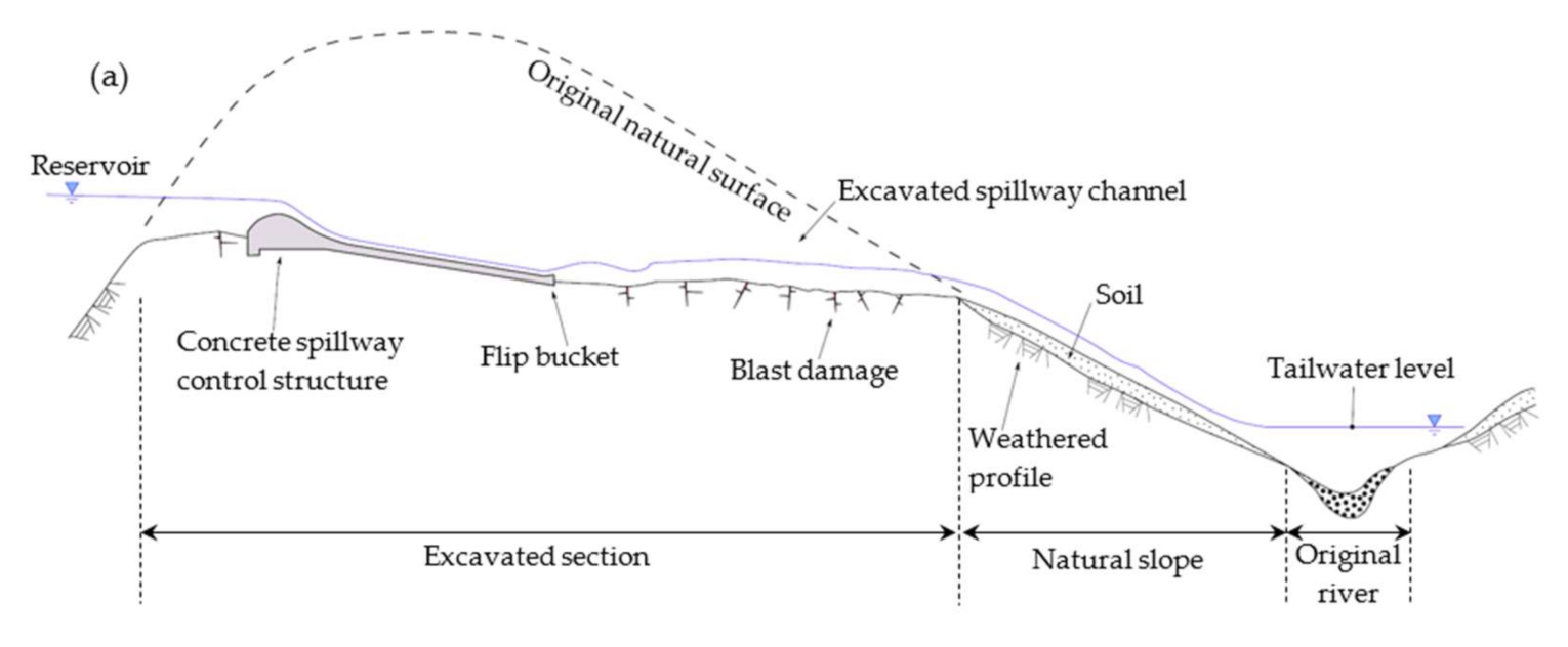
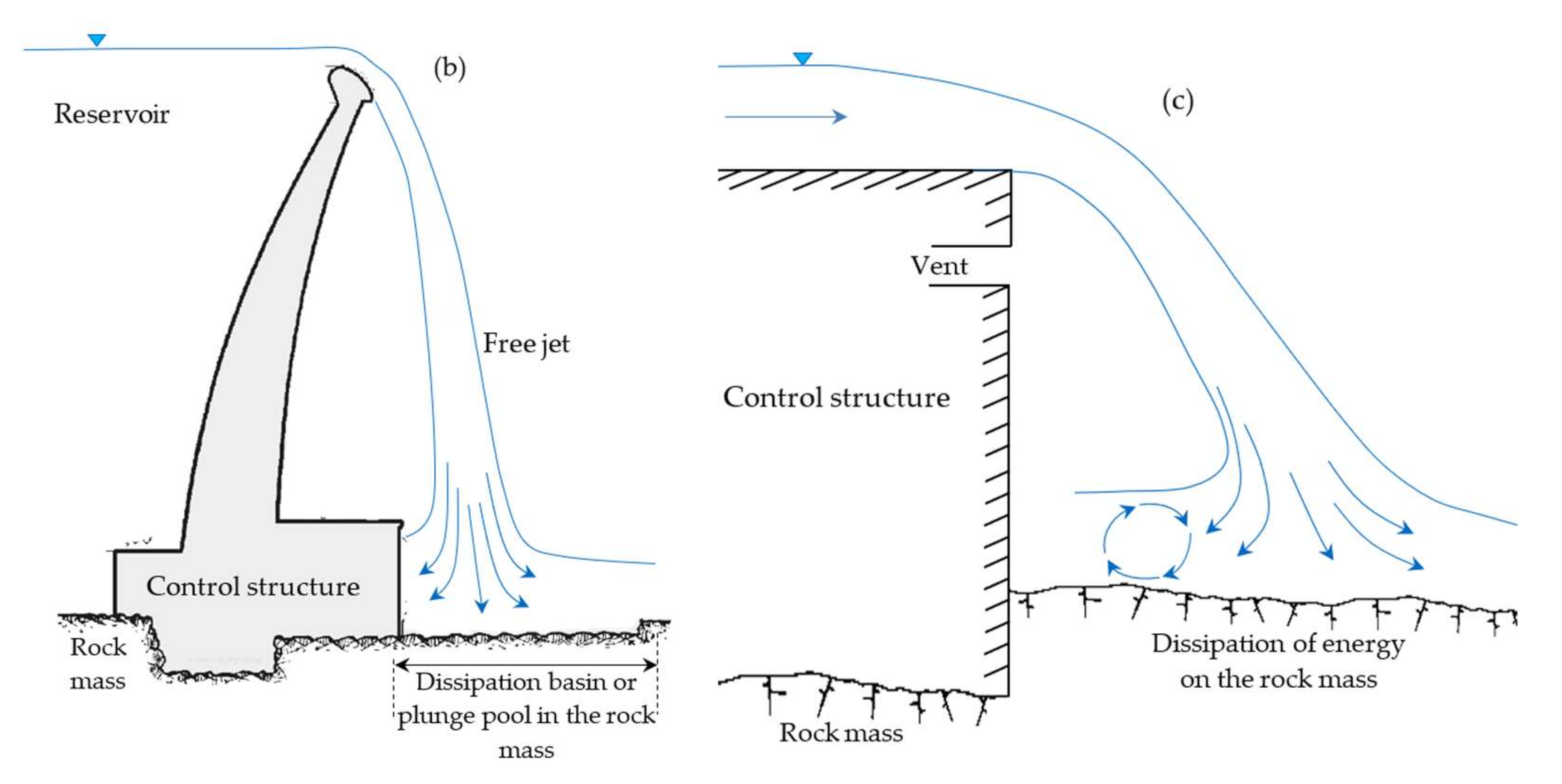
The energy of the discharging water must be dissipated before returning to the river; therefore and depending on the operational mode of the specific spillway, these structures are equipped with a flow channel or a transition zone between the end of the profiled threshold and the final dissipation zone of an evacuation structure (Figure 4a). In other cases, a simple basin, constituting a plunge pool, dissipates the energy immediately at the foot of the spillway (Figure 4b,c). The flow channels dissipate and direct the torrential regime flow toward the final dissipation zone. In this latter case, the observed flow modes differ depending on the nature of the channel, i.e., flows on an inclined slope, hydraulic jumps, flows at knickpoints, and plunging flows into the receiving pool.

Several spillways around the world have been designed and built involving a combination of a discharge channel and a dissipation or stabilization zone. Examples of these combined spillways include the Robert-Bourassa dam spillway (Baie-James, QC, Canada) and the Hell Hole dam spillway (Placer County, CA, USA) [15]. Moreover, in most cases, the dissipation structures are excavated into the rock mass, including the plunge pool or the combination of an evacuation channel and dissipation zone. An important aspect of these unlined spillways is the phenomenon of hydraulic erosion of rock mass. For these spillways, the proper estimation of the erosive force of water is critical.

3. Methods for Estimating the Erosive Force of Water in Spillways

Various methods have been applied to estimate the erosive force of water in erosion processes, and different indices of erosive force have been obtained, including the average shear stress at the bottom surface of a flow channel, the average flow velocity in open channels, the applied stresses inside joints, the block lifting force, and the dissipation of energy from a flow channel.

3.1. Average Shear Stress at the Surface of the Flow Channel

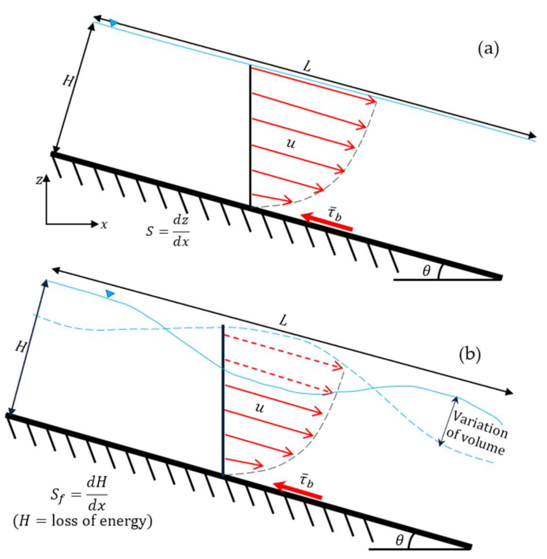
The velocity profile of a fluid is proportional to the applied shear force, and the linear proportionality factor is the dynamic viscosity $\left(\tau = \mu · du/dy\right)$ [5,16]. Given that the viscosity of water is well known, the average shear stress at the bottom surface of a flow channel therefore mainly depends on the variation of flow velocity, which is a function of the nature of the flow. The calculation of shear stress varies, however, depending on the type of flow. The shear stresses for a uniform flow depend on the slope of the flow channel. In the case of non-uniform flow, the total energy gradient is used to estimate the shear stresses in the channel. Figure 5 illustrates possible cases of the distribution and variation of flow velocity. The cases depend on the nature of flow; in the first case, the velocity of a flow is uniform (Figure 5a), whereas the second case has a variable velocity for a non-uniform flow (Figure 5b). Depending on the nature of the flow, shear stress on the bottom of the channel can be estimated using either Equation (1) or Equation (2):

$${\overline{\tau }}_b=\rho · g· R_H · S\cos \theta (\mathrm{Uniform} \mathrm{flow}),$$

(1)

$${\overline{\tau }}_b=\rho · g · R_H · S_f\cos \theta (\mathrm{non}-\mathrm{uniform} \mathrm{flow}),$$

(2)

where $\mu$ is the dynamic viscosity of water, $u$ is the flow velocity, $R_H$is the hydraulic radius, $S$is the slope of the channel equal to $dz/dx$, $x$ is the distance along the channel, $z$ is the elevation above a datum, $g$ is the gravitational acceleration, $\theta$ is the angle of inclination of the channel, and $S_f$ is the total energy gradient equal to $dH/dx= H_f/L · \cos \theta$, and $H_f$ is the energy loss by friction (in m) over distance L, which can be determine using Equation (19) (Section 3.2).

It should be noted that ${\overline{\tau }}_b$ represents the mean hydraulic shear stress on the surface of the channel. The actual shear stress at each point along the channel can always vary because of the presence of relatively rougher parts of the channel. Given this variability, the shear stress term $\left({\overline{\tau }}_b\right)$ is generally replaced by the shear velocity $\left(u_{*}\right),$ which is calculated using Equation (3):

$$u_{*}=\sqrt{\frac{\rho ·g · R_H\sin \theta }{\rho }}= \sqrt{g · R_H\sin \theta } \& {\overline{\tau }}_b=\rho u_{*}^2.$$

(3)

According to Streeter [18], estimating the shear stress in a flow channel is quite complex for turbulent flow because of the variable internal shear stress, which depends on the velocity over the entire depth of the flow profile and the substantial changes along a channel. A simple solution, for this case, is to substitute the dynamic viscosity ($\mu$) with the eddy viscosity ($\eta$) to calculate the shear stress for turbulent flow (Equation (4)) [18]. For this to be possible, the eddy viscosity must be estimated for each flow type, as this parameter is not a constant characteristic of the fluid and varies throughout the profile of the fluid over time. This parameter depends upon the density of the fluid, the velocity gradient, and the mixing length, and it generally varies from point to point in the flow field:

$${\tau }_t= \eta .\frac{du}{dy}$$

(4)

In addition to Equations (1)–(4), expressions exist for estimating the shear stress at the surface of a flow channel.

Table 1. General characteristics of methods for calculating the shear stress at the surface of a flow channel.

Method	Cross-Sectional Shape	Boundary Roughness Distribution
Lundgren and Jonsson (1964)	General	Homogeneous and rough
Flintham and Carling (1988)	Rectangular, trapezoidal	Homogeneous
Pizzuto (1991)	General	Homogeneous
Christensen and Fredsoe (1998)	General	Homogeneous
Khodashenas and Paquier (1999)	General	Homogeneous
Ramana Prasad and Russell Manson (2002)	Rectangular, trapezoidal	Homogeneous
Berlamont et al. (2003)	Rectangular, circular (with or without a flat bed)	Homogeneous
Yang and Lim (2005) and Yang et al., 2004	Rectangular, trapezoidal, circular, V-notch, compounded	Homogeneous
Guo and Julien (2005)	Rectangular	Homogeneous and smooth
Seckin et al. (2006)	Rectangular	Homogeneous and smooth
Severy and Felder (2017)	Rectangular	Homogeneous and smooth

summarizes some existing methods used to calculate this surficial shear stress. Most of these methods are adapted for calculating the local average shear stresses of straight and prismatic flow channels of rectangular, trapezoidal, and circular sections, either with or without a flat or compound bed. Moreover, these methods differ in their assumptions, which can lead to divergent shear stress estimates. We detail some of the methods presented in Table 1 below.

3.1.1. Merged Perpendicular Method

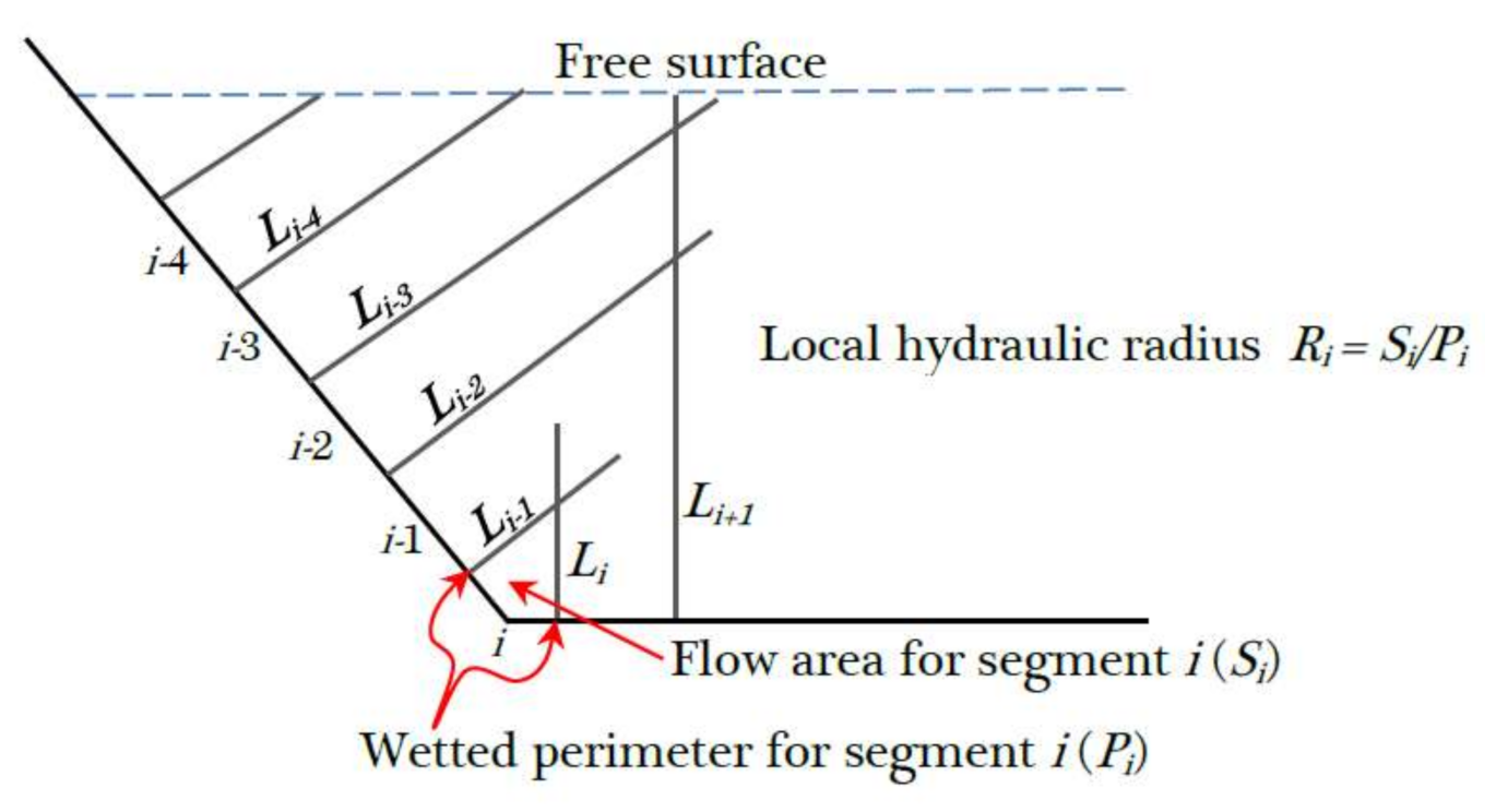
The merged perpendicular method (MPM) is a geometric method for calculating the local shear stress in an irregular cross section of a channel. This method is derived from the normal area method, which relies on the concept of hydraulic radius separation based on the subdivision of a cross-sectional region delimited by walls into three subareas that correspond to the lateral walls and channel bed [19]. The wetted area is then divided into small subareas using the lines normal to the wetted perimeter (Figure 6).

The local shear stress $\left({\tau }_i\right)$ is thus obtained using Equation (5):

$${\tau }_i=\rho · g· R · J_f,$$

(5)

where $R$ is the local hydraulic radius, and $J_f$ is the average energy slope. Subsequently, the average boundary stresses acting on the channel bed and sides are determined by the numerical integration of the local values. However, this method neglects secondary flow structures and the momentum transfer in an irregularly shaped channel. Moreover, the roughness distribution along the wetted perimeter is not considered when the wetted area is divided into subzones.

3.1.2. Ramana Prasad and Russell Manson Method

This method is based on an analytical approach for calculating the percentage of shear force $\left(\%SFw\right)$ carried by the sidewall in prismatic channels of a trapezoidal cross section having a homogeneous roughness [20]. The percentage of shear force is given in terms of the width–depth ratio $\left(b/h\right)$ without accounting for the effect of secondary currents (Equation (6)):

$$\%SFw=\frac{100{\overline{\tau }}_{\left(w\right)}}{{\overline{\tau }}_{\left(w\right)}+ {\overline{\tau }}_{\left(b\right)}\left(\frac{P_{\left(b\right)}}{P_{\left(w\right)}}\right)}=\left\{\begin{array}{c}25\left(4-\frac{b}{h}\right) \frac{b}{h}\le 2\\ \frac{100}{\raisebox{1ex}{$b$}\!\left/ \!\raisebox{-1ex}{$h$}\right.} \frac{b}{h}\ge 2\end{array} \right.$$

(6)

where $P_{\left(b\right)}$ and $P_{\left(w\right)}$ represent the wetted perimeter of the bed and sidewalls, respectively. Knowing $\%SFw$, the following equations are used to determine the shear stress of the bed and the walls of a channel $( {\overline{\tau }}_{\left(b\right)}$ and ${\overline{\tau }}_{\left(w\right)})$:

$$\left\{\begin{array}{c}\frac{{\overline{\tau }}_{\left(b\right)}}{\rho gh{J}_f}=\left(1-0.01\%SFw\right)\left(1+\frac{P_{\left(w\right)}}{P_{\left(b\right)}}\right)\\ \frac{{\overline{\tau }}_{\left(w\right)}}{\rho gh{J}_f}=0.01\%SFw\left(1+\frac{P_{\left(b\right)}}{P_{\left(w\right)}}\right) \end{array}\right.$$

(7)

3.1.3. Yang and Lim Method

This method uses an analytical approach for calculating the distribution of shear stresses in prismatic channels and is based on the concept of excess energy transport over a minimum relative distance within a uniform and fully developed turbulent flow. The relative distance is defined as the ratio of the shortest geometric distance to the energy dissipation capacity (EDC) of the boundary. For a smooth boundary, the characteristic length representing the EDC of the boundary is scaled using the viscous length scale $\left(\nu /u_{*}\right)$ [21], where $\nu$ is the kinematic viscosity of the fluid, and $u_{*}$ is the shear rate. And for an approximate limit, the characteristic length is scaled using the roughness height of the limit. From this concept, Yang and Lim divide the flow zone into subzones on the basis of the shape of the cross section and the roughness of its wetted perimeter; however, secondary currents are not considered. The distribution of average shear stresses along the bed $\left({\overline{\tau }}_{\left(b\right)}\right)$ and side wall $\left({\overline{\tau }}_{\left(w\right)}\right)$ for a smooth trapezoidal channel are determined using Equations (8) through (11):

$$\left\{\begin{array}{c}\frac{{\overline{\tau }}_{\left(b\right)}}{\rho gh{J}_f}=1+\frac{h}{b}\frac{1}{\tan \beta }-\psi \frac{h}{b}\frac{1}{\sin \beta }\\ \frac{{\overline{\tau }}_{\left(w\right)}}{\rho gh{J}_f}=\frac{1}{2}\psi \end{array}\right.$$

(8)

where $h$ is the flow depth, $b$ is the width of the channel bed, $\beta$ is the angle between the sidewall and the water surface, and $\psi$ is the ratio of the EDC of the lateral wall to the EDC of the bottom $\left(\psi =u_{*\left(b\right)}/u_{*\left(w\right)}\right)$. Equation (8) is applicable and valid under the following conditions:

$$\left\{\begin{array}{c}\frac{b}{h}\ge 2\frac{1-\cos \beta }{\sin \beta }\\ \left(1-\psi \cos \beta \right)\le 0\end{array}\right.$$

(9)

The conditions of Equation (9) regarding the applicability of Equation (8) involve the case where the intersection of the dividing lines is located above the water surface in wide channels. In those cases where the dividing lines are located below the water surface in narrow and deep channels, the average stress at the limits is given by Equation (10):

$$\left\{\begin{array}{c}\frac{{\overline{\tau }}_{\left(b\right)}}{\rho gh{J}_f}=\frac{b}{4h}\xi \\ \frac{{\overline{\tau }}_{\left(w\right)}}{\rho gh{J}_f}=\frac{b}{4h{\psi }^2}\xi \end{array} \right.$$

(10)

where $\xi$ is the slope of the dividing line, which is defined as $\xi =\frac{\sin \beta }{\psi -\cos \beta }$. Similarly, for wide channels, Equation (10) is only valid if:

$$\left\{\begin{array}{c}\frac{b}{h}\le 2\frac{1-\cos \beta }{\sin \beta }\\ \left(1-\psi \cos \beta \right)\le 0\end{array}\right.$$

(11)

Thus, for channels having a rough and homogeneous trapezoidal section, the local bed and sidewall average stresses are obtained using Equations (8) and (10), with $\psi =1$, assuming that the dividing lines are the bisectors of the internal base angles of the trapezoid.

3.1.4. Guo and Julien Method

Guo and Julien present a formula for determining the average shear stress of the bed and sidewalls within a smooth rectangular open channel. The method uses conformal mapping, assuming in a first approximation a constant vortex viscosity without considering the effect of secondary currents [22]. In a second approximation, they use two grouped empirical correction factors for the effects of secondary currents, the variable viscosity of the vortices, and other possible effects to calculate the shear stresses (Equation (12)):

$$\left\{\begin{array}{c}\frac{{\overline{\tau }}_{\left(b\right)}}{\rho gh{J}_f}=\frac{4}{\pi }\mathrm{Arctg}\left[\exp \left(\frac{-\pi h}{b}\right)\right]+\frac{4}{\pi }\frac{h}{b}\exp \left(\frac{-h}{b}\right)\\ \frac{{\overline{\tau }}_{\left(w\right)}}{\rho gh{J}_f}=\frac{b}{2h}\left(1-\frac{{\overline{\tau }}_{\left(b\right)}}{\rho gh{J}_f}\right)\end{array} \right.$$

(12)

3.1.5. Method of Seckin et al.

Drawing on the studies by Knight et al., Seckin et al. [23] use nonlinear regression to develop equations derived from an experimental analysis to obtain the percentage total mean shear force on the base and the smooth walls of the wetted perimeter in terms of the width-to-depth ratio. From the percentages of the shear force $\left(\%SFw\right)$, Knight et al. produce equations to determine this average shear stress (Equation (13)):

$$\left\{\begin{array}{c}\frac{{\overline{\tau }}_{\left(b\right)}}{\rho gR{S}_f}=\left(1-0.01\%SFw\right)\left(1+\frac{2H}{B}\right)\\ \frac{{\overline{\tau }}_{\left(w\right)}}{\rho gR{S}_f}=0.01\%SFw\left(1+\frac{B}{2H}\right)\end{array} \right.$$

(13)

where $R$ is the hydraulic radius, $S_f$ is the energy gradient, $B$ is the width of the channel, $H$ is the channel depth, and $\%SFw$ is the percentage of the shear force acting on the walls along a unit of channel length, determined by Equation (14):

$$\left\{\begin{array}{c}\log \left(\%SFw\right)=-1.4026\log \left(B/H+3\right) + 2.6692\\ \mathrm{or} \\ SFw=\exp \left(\alpha \right), in which \alpha =-3.23\log \left(B/H+3\right) + 6.146\end{array}.\right.$$

(14)

Reanalyzing the Knight et al. equations, Seckin et al. [23] use a shifted power adjustment model to find $\%SFw$. They then use various function models to estimate the average wall and bed shear stress of a channel. Seckin et al. [23] apply a rational function model to determine the average bed shear stress, ${\overline{\tau }}_{\left(b\right)}$, and a logistic model to determine the average wall shear stress ${\overline{\tau }}_{\left(w\right)}$. The developed respective equations are:

$$\left\{\begin{array}{c}\frac{{\overline{\tau }}_{\left(b\right)}}{\rho gR{S}_f}=\frac{a+b\left(B/H\right)}{1+c\left(B/H\right)+d{\left(B/H\right)}^2}, where a=0.946, b=0.117, c=0.088 and d=0.0011 \\ \frac{{\overline{\tau }}_{\left(w\right)}}{\rho gR{S}_f}=\frac{a}{1+b\exp \left[-c\left(B/H\right)\right]}, where a=0.011, b=-0.989 and c=0.00034\end{array} \right.,$$

(15)

where $a$, $b$, $c,$ and $d$ represent constants.

3.1.6. Severy and Felder Method

By performing flow tests in a smooth rectangular channel, Severy and Felder [24] develop an equation to calculate the average shear stress of a channel from detailed measurements of flow velocity. They use three approaches to compute the boundary shear stress: the logarithmic law within the inner flow region, the velocity defects law in the outer flow region, and the direct-step method. Relying on the equations of Schlichting and Montes, Severy and Felder develop Equation (16) as a function of a resistance factor to calculate the local shear stress (Equation (16)):

$${\tau }_0=\frac{1}{8}f\rho V^2$$

(16)

where $V$ is the flow velocity, and f is the Darcy-Weisbach friction factor for gradually varying flows, in this case determined by:

$$f=\frac{8 · g · S_f · {\left({\int }_{y=0}^{y=Y_{98}}\left(1-C\right)dx\right)}^2\left(\frac{D_H}{4}\right)}{q_w^2}$$

(17)

where $S_f$ is the energy gradient, $x$ is the longitudinal distance in the direction of flow propagation, $y$ is the perpendicular elevation from the channel bed, $Y_{98}$ is the characteristic flow depth, $C$ is the fraction voids in the flow, $q_w$ is the discharge, and $D_H$ is the hydraulic diameter.

In summary, shear stress is a physical measure of the normal force applied to a channel. Shear stress is intrinsically linked to the nature of the velocity profile and indirectly represents many hydraulic characteristics. Pells [5] selected the mean shear stress of the channel as an appropriate indicator of the erosive force of water. Van Schalkwyk [25] and Pells [5] demonstrated that the amount of observed erosion is well correlated with shear stress. Most researchers hold that the erosion caused by the flow of water in the channel is due to the shear stress exerted by the water at the bottom surface of the flow channel. However, Annandale [7] showed that this notion is only valid for laminar flow; for turbulent flow, the erosion capacity of water depends on the pressure fluctuations exerted by the water rather than shear stress. Moreover, shear stress cannot explain all the probable mechanisms of erosion, including erosion by the dynamic expulsion of blocks recessed in a rock mass or erosion by fragile fracture of the rock mass into small pieces because of turbulent flow. In addition, the average shear stress in the flow channel is a hard-to-estimate parameter that can cause considerable uncertainty in estimates of the hydraulic head under differing flow conditions within the spillways (e.g., hydraulic jump). Most equations used to evaluate this parameter (Equations (5)–(17)) were developed for narrow, smooth-wall flow channels (e.g., pipes) and then applied analytically to other types of channels. Most of these equations have also been developed using assumptions that do not apply to spillway flow channels, including the homogeneity of the shear stress of the flow channel, the non-inclusion of secondary currents in a flow channel, and the non-differentiation of subcritical and supercritical flows. Finally, these methods are based on different assumptions, which can lead to an approach-dependent shear stress estimate. Their use in the cases of flow channels of spillways is therefore highly questionable.

3.2. Average Flow Velocity in Open Channels

The average flow velocity $\left(\overline{u}\right)$ can be calculated on a plane that is perpendicular to the flow direction and is given by the shearing movement in a fluid. This movement leads to the continuous dissipation of energy and depends considerably on the profile of the flow channel surface, the viscosity of the fluid, and the nature of the flow. Various flow resistance coefficients, including the expressions of Darcy-Weisbach, Chézy, and Manning, are known to represent the resistance to flow [26] in the calculation of the average flow velocity.

First, assuming ${\overline{\tau }}_0\propto {\overline{u}}^2$, Chézy [5,26] defined a resistance coefficient to represent the resistance to flow and developed an equation to calculate the average flow velocity as Equation (18):

$$\overline{u}= C\sqrt{R_H.S}; \mathrm{where} C=\sqrt{\frac{\rho .g}{K}}$$

(18)

where ${\overline{\tau }}_0$ is the shear stress, $C$ is the resistance coefficient of Chézy, $\overline{u}$ is the average cross-sectional flow velocity, and $K$ is a probability coefficient or relative roughness coefficient.

Experiments on fluid flow in pipes led Darcy and Weisbach [5,26] to develop a flow resistance coefficient ($f$) and derive an equation for calculating the average flow velocity on a smooth surface. Subsequently, this index was applied to open-channel flows by replacing the diameter of the pipe with an effective diameter representative of the hydraulic radius of a flow channel. The resulting analytical equation is presented as Equation (19):

$$\overline{u}=\sqrt{\frac{8g}{f}}\sqrt{R_H.S_f\cos \theta }; \mathrm{where} H_f=f\frac{L}{d_{eff}}\frac{{\overline{u}}^2}{2g}=f\frac{L}{R_H}\frac{{\overline{u}}^2}{8g },$$

(19)

where $H_f$ is the energy loss by friction (in m) over a distance $L$, and $d_{eff}$ is the effective diameter of channel function for the hydraulic radius of the channel $(d_{eff}=4R_H)$.

Moreover, the calculation of the shear stress in a channel can be performed using Darcy’s coefficient. Equation (20) was developed for this purpose:

$${\overline{\tau }}_b=\rho .{\overline{u}}^2\frac{fL}{H_{f}8}\frac{H_f}{L.\cos \theta }\cos \theta ⟹ {\overline{\tau }}_b=\frac{f}{8}\rho .{\overline{u}}^2$$

(20)

Manning [5,26] calculated the average velocity of a uniform flow from a channel with a flow resistance coefficient of $n$ via Equation (21). It is noted that the Manning coefficient ($n$) depends not only on the shape and roughness of the channel but also on the nature of the flow itself. Hence, this parameter is generally an approximation in calculations, and the known values are specific to river systems:

$$\overline{u}=\frac{1}{n}{R}_H{}^{2/3}{S}^{1/2}; \mathrm{where} n= \frac{R_H{}^{1/6}}{C}=R_H{}^{1/6}\sqrt{\frac{f}{8g}}$$

(21)

In addition to Equations (19)–(21), other equations exist for relating flow velocity to the coefficient of resistance to flow. Knowing that flow resistance is influenced by various parameters, including the shape of the cross section, the non-uniformity of the limits of the flow channel, and the instability of the flow—in addition to the viscosity and the roughness of the walls of a flow channel—flow resistance can be classified into four components: surface or skin friction, form resistance, wave resistance from free surface distortion, and the resistance associated with local acceleration or flow unsteadiness [27]. When the Weisbach coefficient of resistance (f) is applied, flow resistance can be expressed as:

$$f=F \left(Re, K, {\eta }_0, N, Fr, U\right)$$

(22)

where $F$ represents a function, $Re$ is the Reynolds number, $K$ is the relative roughness coefficient (usually expressed as $k_s/R$, where $k_s$ is the equivalent wall surface roughness and $R$ is the hydraulic radius of the flow), ${\eta }_0$ is the cross-sectional geometric shape, $N$ is the non-uniformity of the channel in both profile and plan, $Fr$ is the Froude number, and $U$ is the degree of flow unsteadiness. The parameters of this equation are independent, and the four resistance components (surface, form, wave, and unsteadiness) interact nonlinearly so that any linear separation and combination are artificial.

The internal and external laws of the boundary layer theory are used to explain some components of flow resistance and better define the flow resistance with respect to these parameters. The theory of the boundary layer refers to a zone in a flowing fluid where the viscous effects are as important as the effects of inertia in terms of magnitude. Within this layer, the tangential velocity with respect to the wall changes very quickly, having no velocity at the wall and a greater-than-zero velocity outside this layer. Thus, the boundary layer represents the interface zone between a body and a surrounding fluid.

According to this theory, the distribution of the velocity (u) along the normal direction (y) to the wall is correctly described by the internal law (or the law of the wall) where the viscous effect dominates and the external law (or velocity defects low) [16,28]. The expressions defined by these laws are:

$$\frac{u}{u_{*}}=F\left(y^{*},k^{*}\right) \mathrm{where}: y^{*}=\frac{u^{*}y}{\nu }, \mathrm{and}$$

(23)

$$\frac{U-u}{u_{*}}=F\left(\frac{y}{\delta },H_s\right)$$

(24)

where $u_{*}$ is the shear velocity (Equation (3)), $k^{*}$ is the Von Karman’s constant, $y^{*}$ is a constant equal to $u^{*}y/\nu$, $\nu$ is the kinematic viscosity of the fluid, $U$ is the free stream velocity at the far end of the outer law, and $\delta$ is the boundary layer thickness. $H_s$ is often called a shape factor, a nondimensional parameter associated with the pressure gradient and Reynolds number, and it is usually expressed as the ratio between the displacement and momentum thicknesses of the boundary layer.

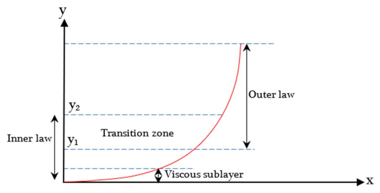
Knowing that the inner and outer laws are not mutually exclusive, there is a region of overlap between the lower limit of the outer law and the upper limit of the inner law (Figure 7). To characterize this transition zone, researchers have developed equations to satisfy both laws. Rouse presented a logarithmic function that applies to the laws expressed by Equations (23) and (24), and the power-law distribution of Chen is also used [27]. These equations are presented respectively in Equations (25) and (26). More information on the logarithmic function and power-law distribution can be found in of Nezu et al. [29]:

$$\frac{u}{u_{*}}=c_1\log y^{*}+c_2, \mathrm{and}$$

(25)

$$\frac{u}{u_{*}}=c_3{\left(y^{*}\right)}^m,$$

(26)

where $c_1$, $c_2,$ and $c_3$ are constants for a given channel. From these equations, the open-channel resistance can be derived and extended from the resistance of a uniform flow in a circular rigid pipe.

The closest open channel counterpart of a circular pipe (besides a half circle) is the two-dimensional (2D) wide channel. With the shape factor held constant for 2D wide channels or circular pipes, Equations (23) and (24) imply that, referring to Equation (22), the resistance to a steady uniform flow is solely a function of the Reynolds number $Re$ and the relative roughness $K=k_s/R$, provided that the Froude number is not high and its effect is negligible. Hence, the resistance factors become:

$$f, \frac{n}{R^{1/6}},\frac{C}{\sqrt{g}}, =F\left(Re, \frac{K_s}{R}\right),$$

(27)

where $k_s$ is the equivalent wall surface roughness, and $R$ is the hydraulic radius.

From Equation (27), various resistance coefficients in the form of Darcy-Weisbach can be derived, depending on $Re$:

-

For a uniform and regular laminar flow with a $Re<500$, the resistance factor is obtained as

$$f=K_L/Re ,$$

(28)

where $K_L=24$ for wide channels and $K_L= 16$ for circular pipes.

-

For $700<Re<25,000$, the resistance factor for a smooth pipe (and often used as an approximation for wide channels) is

$$f=0.224/R{e}^{0.25} .$$

(29)

-

For $Re>25,000$, the resistance factor becomes

$$\frac{1}{\sqrt{f}}=-K_1\log \left(\frac{k_s}{K_{2}R}+\frac{K_3}{4Re\sqrt{f}}\right) ,$$

(30)

where $K_1$, $K_2,$ and $K_3$ represent Colebrook-White coefficients for a regular uniform flow in open channels with a rigid impermeable limit [27].

These Colebrook-White coefficients are implicit in the determination of f. To overcome this drawback, Churchill [30] and Bray [31] assumed full flow in a pipe to then propose an equation for calculating the flow resistance as:

$$f= \frac{1}{4}{\left[-\log \left(\frac{k_s}{14.8R}\right)+\frac{5.76}{{\left(4R_e\right)}^{0,9}}\right]}^{-2}.$$

(31)

From Equation (31), Yen suggested a formula to calculate the flow resistance for large open channels having a $Re>3000$ and a $k_s/R<0.05$ [27]:

$$f= \frac{1}{4}{\left[-\log \left(\frac{k_s}{12R}\right)+\frac{1.95}{R_e{}^{0,9}}\right]}^{-2}.$$

(32)

For Equations (27)–(32), flow resistance is determined in terms of limit shear, that is, from the perspective of the relationship between force and momentum. This concept determines the flow resistance of open channels in terms of the slope of the impulse resistance along a channel for a channel cross section. However, other work has shown that resistance to flow can also be examined from the concept of energy in terms of the energy loss when a fluid moves across a surface, as well as in terms of the energy slope or, more precisely, the gradient of the mean motion of the dissipated energy. Yen and Akan [32] suggest the rather than applying Equation (28), Equation (28) can be used for the momentum equation of laminar sheet flow under rain-full conditions with an intensity i:

$$f_m=\left[24+660{\left(\frac{i}{\sqrt[3]{g\nu }}\right)}^{0.4}\right]\frac{1}{Re}.$$

(33)

In summary, Equations (19)–(21) indicate that the average flow velocity is directly related to the pressure that is applied to the surface of a rock mass or inside a joint. Therefore, the average flow velocity is a key element for determining the specific forces that are applied to a rock mass. However, the average flow velocity is sensitive to the problem of “non-uniqueness” in the field of hydraulic erosion. Pells [5] and Van Schalkwyk [25] reported that the average velocity could not be used as a representative value in hydraulic hazard parameters for erosion prediction. Moreover, the average flow velocity is proportional to the flow resistance coefficient, which can be defined by knowing the roughness of the flow channels and spatial variation along the flow channel. To specify the flow resistance, the resistance coefficients of Darcy-Weisbach, Chézy, and Manning are used to estimate mean flow velocity. The equations detailed above (Equations (28)–(33)) illustrate the diverse means of determining resistance coefficients, and this diversity of approaches can explain the confusion among users and the inconsistencies among the produced values for the resistance coefficients. The application of these flow resistance coefficients in flood spillways also remains uncertain. Indeed, the theory of the boundary layer served as a basis in the development of some resistance coefficients and this theory would be less effective for flow channels with very rough surface. Under the flow conditions considered for rough unlined spillways, the roughness elements may exceed the thickness of the boundary sublayer (fully turbulent flow) and the velocity profile is fully developed, that is, the thickness of the boundary layer is equal to the depth of the outflow [5]. According to Yen [27], the inner law region (Figure 7) below the transition zone is generally thin and it is difficult to measure velocity, especially when the roughness of the wall is large.

The multiple equations established to determine the resistance to flow of a channel fluid represent the derivative and the extent of the resistance of a uniform and constant flow in a rigid circular pipe. These coefficients are approached either from the perspective of impulse resistance (resistance slope) or energy loss (energy movement gradient). These various Darcy-Weisbach, Manning, and Chézy resistance coefficients can be related (Equation (27)), and there is no clear theoretical advantage of one coefficient over the other. The C (Chézy) coefficient is, however, the simplest to use, although there is no generally accepted table or figure of C values. The n (Manning) coefficient has the advantage of being nearly constant and almost independent of flow depth, Reynolds number, or $k_s/R$ for fully developed turbulent flow on a rigid and rough surface [27]. Determining the resistance coefficient values by Manning, obtained from field data, relies on the head loss energy concept applied to channel reaches. The f (Darcy-Weisbach) coefficient has the advantage of being directly linked to the development of fluid mechanics, and there are known values for this coefficient, the most reliable source for the values of f being the Moody diagram. Generally, f is regarded as a point value related to the velocity distribution, although some hydraulic engineers extend it to cross-sections or reach values and consider it as an energy loss coefficient. Thus, it appears appropriate to refer to the Darcy-Weisbach f for point resistance, whereas Manning’s n can serve for cross-sectional and reach resistance coefficients. Previous field experiments suggest that n is a simpler coefficient when accounting for the effects of other parameters beyond the Reynolds number and relative roughness, as well as from a fluid mechanics perspective. A drawback of Manning’s formula is that it is dimensionally non-homogeneous [27].

In general, these flow resistance coefficients are not representative of the roughness of a flow channel of a spillway; for example, the Darcy-Weisbach coefficient was specifically developed for pipes having a smooth surface and was then analytically modified for use in open-channel flows. Manning’s coefficient is more applicable to river systems; however, the roughness values of an uncoated channel of high-speed spillways is generally greater than those estimated from river systems. Moreover, in practice, the resistance varies among points, in particular along the flow channels of the spillway, whereas the resistance coefficient for a cross section or a range of channels is a spatially weighted average of local resistance. Yen [27] concludes that despite the success of resistance coefficients in presenting complex physical processes in flows, much remains to be studied, including the effects of channel geometry and flow instability on resistance to the flow.

3.3. Applied Stresses inside Joints and the Block Lifting Force

Bollaert [6,8,33,34] estimated the hydraulic load on the rock mass by considering the hydrodynamic tensile load of the joints, represented by the stress intensity factors in the various erosion mechanisms. First, erosion is defined as resulting from instantaneous brittle fracture (hydrofracturing), where the hydraulic head is defined by a stress factor$\left(K_I\right)$. This index represents the stress induced by the water pressure inside the joints and, hence, the brittle fracturing occurs when the intensity of the stress in the joints, owing to fluctuating pressure, is greater than the resistance of the rock mass (Figure 2). The semi-analytical index developed by Bollaert is presented in Equation (34):

$$K_I=0.8 · P_{max} · F · \sqrt{\pi · L_f},$$

(34)

where $0.8.P_{max}$ represents 80% of the maximum instantaneous dynamic pressure in the diving tank, $F$ is the correction factor, which depends on the types of cracks when it is persistent, and $L_f$ is the total length of a joint.

In cases where brittle fracture is not likely, another mechanism dominates, i.e., fatigue erosion or the progressive hydrofracturing of a rock mass. If the intensity of the stresses in the joints does not exceed the fracture toughness of the rock mass, the existence of a continuous fluctuating pressure in the joints can ultimately lead to the failure of the rock because of fatigue (Figure 3). In this context, Bollaert considered the hydraulic head via a stress intensity amplitude factor$\left(\Delta K_I\right)$, which corresponds to the difference in intensity of maximum and minimum stresses inside a joint or, in a rough estimation, could be considered equal to 40% of$K_I$.

In a fractured rock mass characterized by a system of joint sets that form a block assembly, erosion occurs by the dynamic expulsion of the blocks through water pressure as a lifting force. Bollaert [6,8,33,34] estimated this load by considering the essential lifting force of the individual block. This lifting force can be expressed as a dynamic impulse index that is obtained by the temporal integration of the net forces applied to a block. These forces include the force applied on top of the block $(F_o)$, the lifting force beneath the block $\left(F_u\right)$, the submerged weight of the block $\left(G_b\right),$ and the friction along the sides of the block $(F_{sh}$) (Figure 1). The equation developed to define the lifting force of an individual block is presented in Equation (35):

$$I={\int }_0^{\Delta tpulse}\left(F_u-F_o-G_b-F_{sh}\right) · dt=m · V_{\Delta tpulse},$$

(35)

where $V_{\Delta tpulse}$ is the velocity of the fluid in the joint, and $m$ is the mass of the rock block.

In summary, the Bollaert index [6,8,33,34] defining the erosive force of water on a rock mass illustrates effectively the three mechanisms of erosion and the importance of the pressure dynamics in hydraulic erosion. These indices ($K_I$ and $I$) illustrate the erosive force of water, as they are developed on the basis of various erosion mechanisms of a fractured rock mass. To correctly apply these indices, however, some considerations must be addressed. First, these indices are not applicable to other flow modes at spillways; for example, they do not apply to parallel flow along the bottom of the channel and hydraulic jumps. Moreover, the first two factors depend mainly on the maximum instantaneous dynamic pressure$\left(P_{max}\right)$. This pressure depends in turn on the average velocity of the jet at the impact point $\left(V_j\right)$ and the dynamic pressure coefficient. The latter coefficient is obtained by multiplying the quadratic mean pressure coefficient $\left(C_{pa}^{’}\right)$ by a pressure amplification factor in the joints$\left({\mathsf{\Gamma }}^{+}\right)$ and then adding a mean dynamic pressure coefficient$\left(C_{pa}\right)$. The expression developed to calculate the instantaneous dynamic pressure is presented in Equation (36):

$$P_{max}={10}^{-6}\rho · \left(C_{pa}+{\mathsf{\Gamma }}^{+} · C_{pa}^{’}\right) · \frac{V_j^2}{2g},$$

(36)

where the parameters $C_{pa} and C_{pa}^{’}$depend on the toughness of the rock mass and are obtained experimentally. Nonetheless, the toughness of the rock mass is an irrelevant criterion for the erosion of fractured rocks, and no setup can determine the toughness of a rock [7]. The parameter $L_f$ in Equation (34) represents the total length of a single joint. However, from the field data obtained by Pells [5], this parameter does not adequately represent the geometry of an entire erosion zone because it is determined using a reduced physical model that is not representative of a fractured rock mass.

The second index developed by Bollaert, the lifting force of a block, also includes some nuances as to its reliability for estimating the erosive force of water. The first is that the index does not consider the shear strength along the sides of the blocks$\left(F_{sh}\right)$. Moreover, according to Figure 1, the net lifting force of a block also depends on the joint openings. As the openings become larger, the amount of water seeping into the joints increases, which directly influences the pressure below the blocks. Therefore, this index of dynamic block uplift once again ignores an important parameter contributing to the resistance of a block to erosion. Furthermore, the indices developed by Bollaert [6,8,33,34] apply only to plunging jets, and, hence, these indices are not applicable to other flow conditions. As a result, they must be improved to not only determine the erosive hydraulic force of the plunging jets for which they have been developed but also for their application to other flow modes.

3.4. Indices of Energy Dissipation

The dissipation of energy in spillways depends mainly on the flow condition, which is primarily a function of spillway shape. Therefore, hydraulic powers should vary among flow conditions. Several authors have thus developed expressions to calculate the dissipation of energy in relation to the variation of the total energy gradient$\left(\frac{dE}{dx}\right)$ to define the erosive force of water within spillways. Van Schalkwyk [25] evaluated the energy dissipation for plunging flows. Annandale [4] attempted to develop an expression for estimating the energy gradient for calculating energy dissipation in plunging jets, hydraulic jumps, and knickpoint flows. Similarly, Pells [5] developed expressions to determine the variation of the hydraulic gradient for plunging jets and hydraulic jumps.

Van Schalkwyk [25] used the ratio between the total power of flow $\left(T\right)$ and the surface on which it is dissipated $\left(A\right)$ to estimate the energy dissipation, following Equation (37):

$$P= \frac{T}{A}, \mathrm{where} T=\rho gQ,$$

(37)

where $Q$ is the water flow rate, and $H$ is the total head.

Equation (37) was then applied to different flow modes observed at spillways to estimate the energy dissipation of each. Accordingly, energy dissipation for an inclined channel was calculated on the basis of the power loss over a distance. The energy released owing to variations of the total head corresponds to the slope of the hydraulic gradient, and the produced equation is presented in Equation (38):

$$P=\rho gqS, \mathrm{where} S= \frac{dH}{dx} \mathrm{and} \frac{dT}{dx}=\rho gQS,$$

(38)

where $q$ is the flow rate per unit length of channel width $\left(q=Q/B_f\right)$, and $B_f$ is the channel width.

Van Schalkwyk [25] then reformulated Equation (37) to calculate energy dissipation for a plunging flow by selecting a coefficient of 3 as the energy gradient for the plunging jet. Equation (39) presents the modified Equation (37) for calculating the energy dissipation at a plunging flow:

$$P=3gq.$$

(39)

Equations (38) and (39), developed by Van Schalkwyk, are only applicable to inclined uniform flow and plunging jets; however, some considerations should be noted. For example, the flow within the inclined flow channels of spillways is not uniform; and using a coefficient of 3 as the energy gradient for a plunging jet needs to be evaluated further, as the energy gradient of a plunging jet is highly variable. These equations are therefore not sufficiently comprehensive to evaluate the erosive force of water within spillways.

Annandale [4] also proposed equations for calculating the erosive force of water within spillways. When the density of water, the unit flow rate, and the energy loss of a flow are accounted for, the resulting equation is:

$$P= \gamma · q · \Delta E,$$

(40)

where $\Delta E$ is the energy loss depending on the type of flow, and $q$ is the specific discharge rate equal to the flow rate divided by channel width. Considering a flow channel with a length $\left(w\right)$ and depth of water $\left(d\right)$ that is measured perpendicular to the flow direction, the unit discharge rate is calculated using Equation (41):

$$q=\frac{Q}{w}=\frac{\overline{u}\times A}{w}= \frac{\overline{u} · w · d}{w}= \overline{u} · d .$$

(41)

From Equation (40), Annandale [4] developed several equations to estimate the erosive hazard parameter for various flow modes at spillways, including for lunging jets, hydraulic jumps, and knickpoint flows.

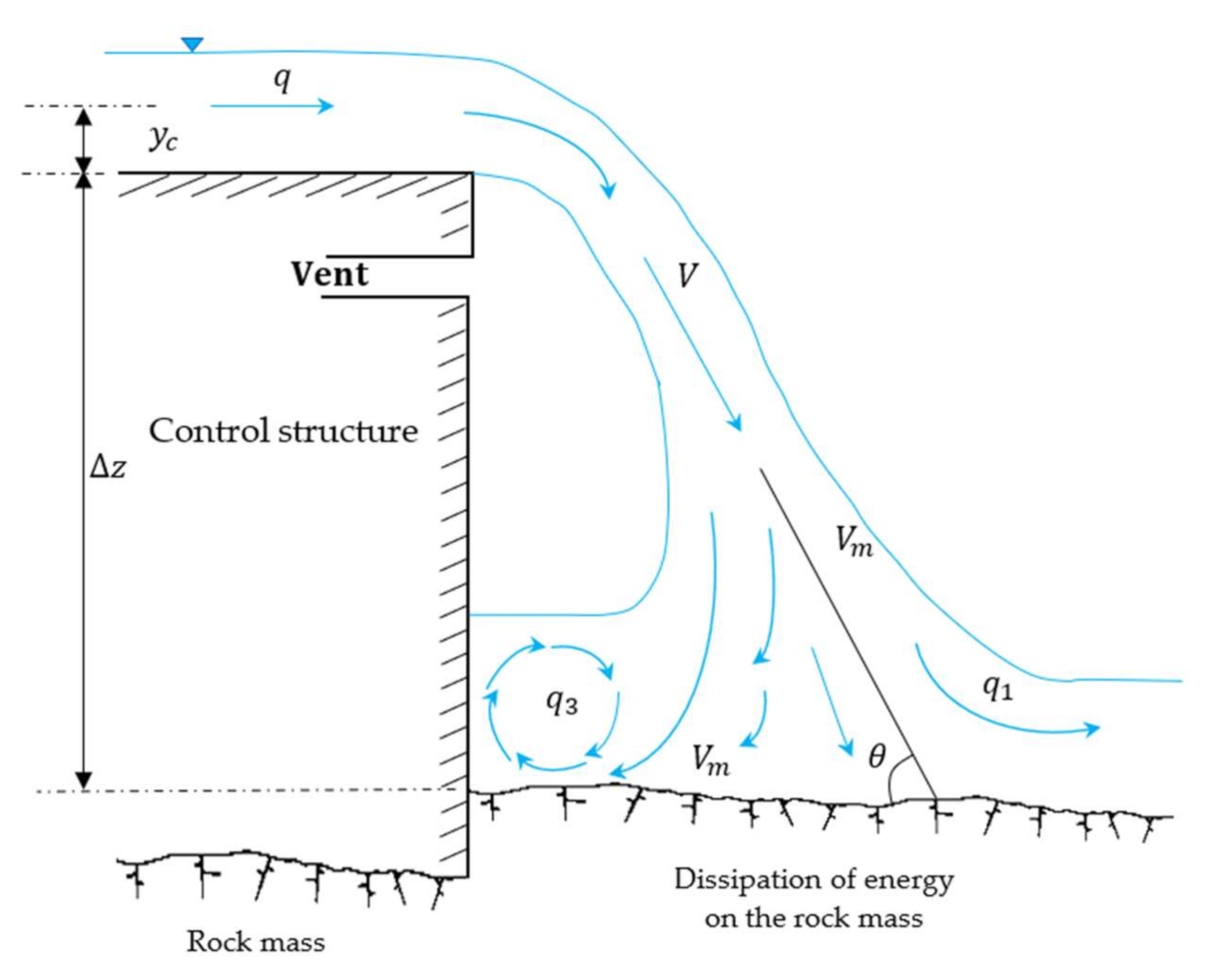
In regard to plunging jets, Figure 8 shows the characteristic parameters considered by Annandale, where energy loss$\left(\Delta E\right)$ is calculated as a function of specific discharges$\left(q_1 and q_3\right)$. From this, Annandale [4] developed Equations (42) and (43) to determine the energy dissipation for a plunging jet:

$$P=\gamma · q · y_c· \left(\frac{\Delta z}{y_c}+\frac{3}{2}-\frac{y_l}{y_c}-\frac{1}{4}\left(\frac{3}{2}+\frac{\Delta z}{y_c}\right){\left(1+\frac{1.06}{\sqrt{\frac{\Delta z}{y_c}+\frac{3}{2}}}\right)}^2\right) (\mathrm{depends} \mathrm{on} q_1),$$

(42)

$$P=\gamma · q · \frac{v^2}{8g}{\left(1+\frac{1.06}{\sqrt{\frac{\Delta z}{y_c}+\frac{3}{2}}}\right)}^2 (\mathrm{depends} \mathrm{on} q_3),$$

(43)

where $y_c$ is the critical depth of the jet, $\Delta z$ is the height of the spillway, $v$ is the average flow velocity, and $y_l$ is the downstream flow depth.

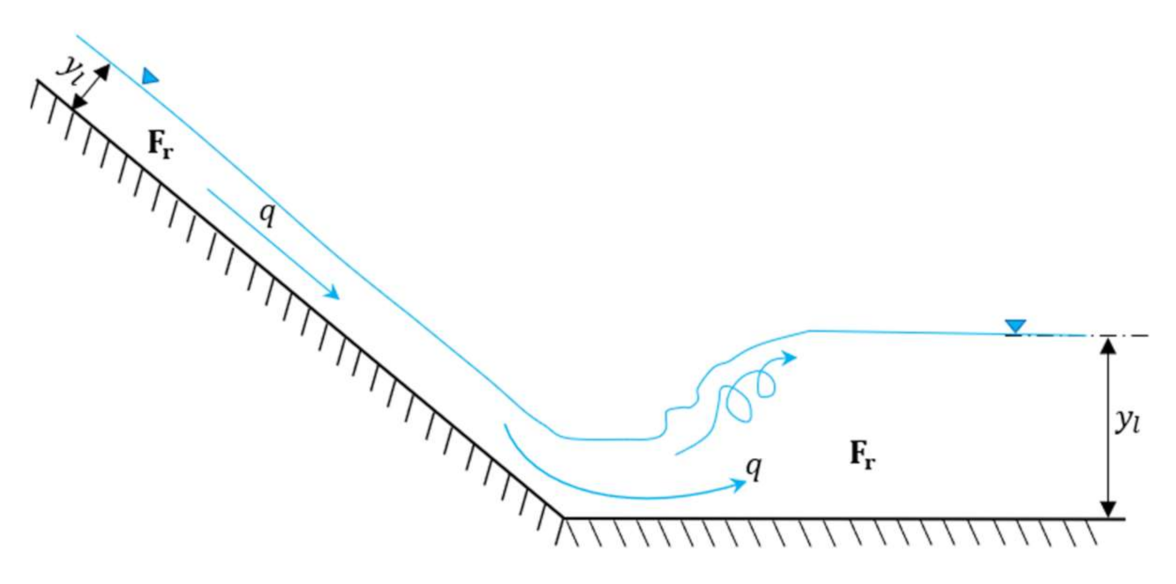
For a fluid flowing as a hydraulic jump, the significant parameters considered by Annandale for this type of flow are represented in Figure 9, and the relevant equation is presented in Equation (44):

$$P=\gamma · q\left(y_l+\frac{q^2}{2g{y}_l^2}-\frac{y_l}{2}\left(\sqrt{1+8F_r{}_l^2}-1\right)-\frac{q^2}{2g}-\frac{4}{y_l^2{\left(\sqrt{1+8F_r{}_l^2}-1\right)}^2}\right).$$

(44)

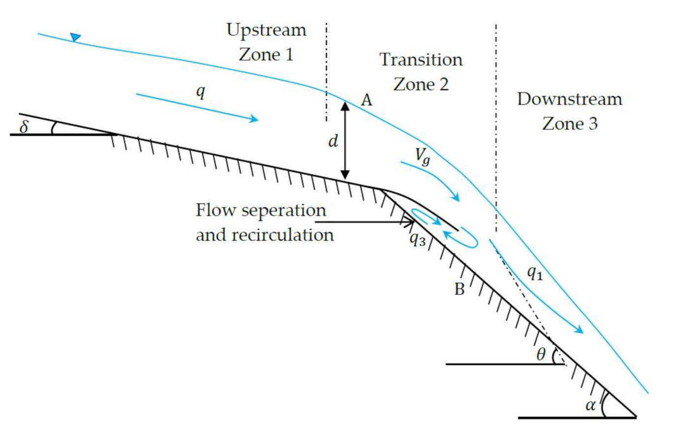
According to Annandale [4], the maximum dissipation of a knickpoint flow occurs at the point where the angle of the flow channel changes from a low to a steep angle (Figure 10).

Equation (45) is subsequently used to estimate the energy dissipation for a knickpoint flow:

$$P=\gamma · q\left(\frac{1+\cos \left(\theta -\alpha \right)}{1-\cos \left(\theta -\alpha \right)} K_l\left(\frac{v_g^2}{2g}\right)+ S_f · L\right),$$

(45)

where $K_l$ is a probability coefficient estimated at 1 (on the pretense that it provides consistent results), $\theta$ is the angle approximated by superimposing the theoretical ogee shape onto the channel bed geometry, and $\alpha$ is the slope angle of the channel.

The equations used by Annandale [4] to estimate the energy dissipation for various flow modes lack clarity and detail and have thus been criticized; for example, Pells [5] points out that the Annandale equation ignores the hydraulic jump length $\left(\Delta x\right)$ in the definition of flow dissipation (i.e., the expression is $\rho gq\Delta E$ rather than the correct form$\rho gq\frac{\Delta E}{\Delta x}$). This issue was modified by Annandale [7] by using $\Delta x=1 \mathrm{m}$ and mentioning that this value provides a conservative estimate in the absence of effective data. Henderson [35] demonstrated that the length of dissipation is a significant parameter at $\Delta x=6y_2$ ($y_2$ is the height of the water downstream of the flow channel), where the Froude number lies in the $4.5<F_r<13$ range. Moreover, for the specific discharge rate between 1 and 50 m² s⁻¹, Annandale’s analytical solution overestimates the unit energy dissipation [5]. This dissipation length is also ignored in the analytical solution of the unit power dissipation of a knickpoint flow condition and downstream of a jet. Finally, the equation provided by Annandale [4] for calculating the energy dissipation of the back roller (Equation (43)) disregards the length of the energy dissipation. These criticisms therefore discourage the use of the Annandale equations in this context.

Pells [5] developed Equation (46) to calculate the erosive force of water in the flow channel of the spillways:

$$\Pi =\rho gQ\left( \frac{P_r}{\rho g}+\frac{{\overline{u}}^2}{2g}\right),$$

(46)

where $P_r$ is the water pressure, and $\rho$ is the density of water.

The dissipation of the fluid energy represents the velocity at which the power is expended, corresponding to the flux gradient. Hence, by multiplying the slope of the total energy line by $\rho gQ$, a simplified form of the energy dissipation equation is presented in Equation (47):

$${\Pi }_{UD}=\rho · g · q\frac{dE}{dx}.$$

(47)

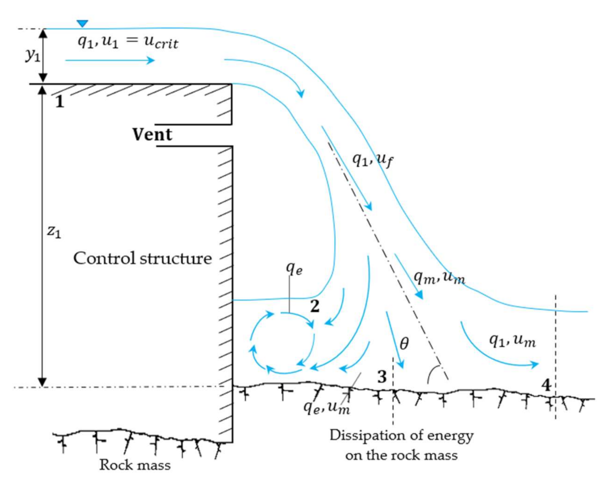
From Equation (47), Pells [5] developed equations related to the various flow modes found in spillways. Figure 11 illustrates the different parameters that are considered in plunging flow. From these parameters, the estimation of the energy loss in plunging flows over distance (between points 1 and 4 of Figure 11) is presented in Equation (48):

$$\Delta E=z_1+y_1\left(\frac{3}{2}-\frac{2}{\sqrt{2}\alpha +\frac{3}{2}}-\frac{{\left(\sqrt{2}\alpha +\frac{3}{2}\right)}^2}{8}\right),$$

(48)

where $z_1$ is the height of the spillway, $y_1$ is the height of the water from the surface of the discharge point, and $\alpha$ is a coefficient depending on $z_1$ and $y_1$ $\left(\alpha =\sqrt{\frac{3}{2}+\frac{Z_1}{y_1}}\right)$. By combining Equations (47) and (48), Pells [5] proposed an equation (Equation (49)) to calculate the energy dissipation for a plunging flow:

$${\Pi }_{UD}=\rho · g · q_1\frac{dE}{dx}=\frac{\rho · g · q_1}{\sqrt{2z_1{y}_1}}\left[z_1+y_1\left(\frac{3}{2}-\frac{2}{\sqrt{2}\alpha +\frac{3}{2}}-\frac{{\left(\sqrt{2}\alpha +\frac{3}{2}\right)}^2}{8}\right)\right].$$

(49)

Subsequently, Pells [5] estimated the energy dissipation for a hydraulic jump flow, a flow characterized by an abrupt change in the flow regime. By knowing the initial velocity and depth, the downstream depth of the flow can be calculated. Thus, it is possible to calculate the variation in velocity and the energy loss between two points (from upstream to downstream). The resulting equation is presented in Equation (50). By combining Equations (47) and (50) and applying a distance about $6y_2$ between points (for 4.5 < $F_{r1}^2$ < 13) [35], Equation (51) allows calculating the energy dissipation for a hydraulic jump:

$$\Delta E=y_1+\frac{q^2}{2g{y}_1^2}-\frac{y_1}{2}\left(\sqrt{1+8F_{r1}^2}-1\right)-\frac{4q^2}{2g{y}_2^2{\left(\sqrt{1+8F_{r2}^2}-1\right)}^2},$$

(50)

$${\Pi }_{UD}=\frac{\rho · g · q}{6y_2}\left(y_1+\frac{q^2}{2g{y}_1^2}-\frac{y_1}{2}\left(\sqrt{1+8F_{r1}^2}-1\right)-\frac{q^2}{2g{\left(\frac{y_1}{2}\left(\sqrt{1+8F_{r2}^2}-1\right)\right)}^2}\right),$$

(51)

where $y_2$ is the height of the water downstream of the flow channel.

In summary, the analytical methods for estimating energy dissipation presented by Pells [5] appear to be more reliable than other approaches. Generally, energy dissipation is a widely used index for evaluating the hydraulic erodibility of a rock mass and is used to represent the erosive force of water in most modes of hydraulic erosion assessments. These methods are Π_UD vs. RMEI [5], Π_UD vs. eGSI [9], and P = f(K_h) [4,7,11,13,25]. This energy dissipation index is used because of its simplicity rather than its effectiveness in representing the erosive force. That is, owing to the absence of a reliable index and the complexity of estimating the actual erosive force of water within a spillway, energy dissipation is used as a simple indicator of erosive hydraulic force. According to Pells [5], the use of energy dissipation by itself is common, although it does not present all the complexities of the erosion process; an infinite number of combinations of spillway geometry and flow modes can be potentially associated with a given measure of energy dissipation. Moreover, a direct interpretation of energy dissipation infers that it is not a direct measurement of erosive capacity but rather represents energy loss linked to the conservation of heat and not to the work performed. It is thus evident that there exists the need to develop an improved index for calculating the erosive force of water to assess the erosion of a fractured rock mass.

4. Discussion

The indices reviewed in this paper were developed to represent the erosive force or hazard parameter of water for the purpose of determining rock erosion in the spillways of hydroelectric projects. The previous sections exhaustively discuss the advantages and disadvantages of each method for estimating the erosive force of water.

The non-representativeness of average velocity $\left(\overline{u}\right)$ is linked to its sensitivity to the problem of “non-uniqueness” in the realm of hydraulic erosion. In short, the average shear stress at the surface of the flow channel $\left({\overline{\tau }}_b\right)$ is designated as being representative of the hazard parameter of the water within the spillways. However, shear stress cannot explain all possible erosion mechanisms within the spillways, e.g., erosion via the dynamic removal of blocks or erosion by the brittle fracture of large blocks into smaller blocks. This inability to fully explain the erosion mechanisms and the difficulty of estimating shear stress are among the limitations when using this factor to calculate the erosive force of the water. Energy dissipation as an erosive force does not include all the complexities of the erosion process and is used to calculate the erosive hazard parameter of water mainly because it is simple to determine, not because of its representativeness.

In regard to the semi-analytical solutions of Bollaert [6,8,33,34], they can be used for estimating the erosive force of water as they better explain the principles behind the different mechanisms of hydraulic erosion of rock mass; however, there are some criticisms of these indices. The first index, developed on the basis of the stress applied to joints$(K_I$), includes parameters that are difficult to determine for a rock mass. Among them, $L_f$ (the total length and shape of the joints) is not representative, as it was developed using a scale model that is not representative of the fractured zone of a rock mass. In addition, uncertainty is associated with the determination of the empirical variables, including $C_{pa}, C_{pa}^{\prime },\mathrm{and} {\Gamma }^{+}$. The second index, the dynamic impulse of the blocks$\left(I_{impuls}\right)$, also disregards some important parameters that influence the accuracy of the model, such as the shear strength $\left(F_{sh}\right)$ along the block sides. Another essential parameter for estimating the lifting force of a block (see Figure 1) is the opening of the joints, a parameter directly influencing the pressure below the blocks, the latter an important parameter neglected by the lifting force of the blocks. Generally, the most important parameter for estimating the Bollaert indices is the maximum dynamic pressures or the peak pressures applied within joints. However, Pells [5] mentions that the pressure fluctuation follows a Gaussian distribution; thus, no pressure peak is observed in the joints. Thus, these indices are only applicable to plunging flows, and modifying the existing indices becomes essential.

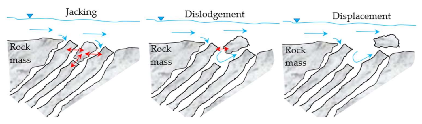
Our review found that the main shared factor related to the indices used to represent the erosive force is the pressure applied to the discontinuities of the rock mass. Among all the mechanisms controlling hydraulic erosion, erosion by dynamic block removal appears to be the most common erosion mechanism of fractured rock masses, as evidenced by several cases of erosion observed at the flow channels of spillways around the world. These cases of erosion by removal of the blocks mainly concern the spillways with inclined flow channels. Figure 12 shows in detail the mechanism of erosion by removal of the blocks in the inclined flow channels of the spillways. This remark therefore emphasizes that different flow modes within spillways share similar dynamics of erosion; hence, the dynamic expulsion index of the blocks seems more suitable than the other indices to represent the erosive force of water. Nonetheless, the dynamic expulsion index must be improved, as it neglects important parameters, including shear strength and joint opening. Moreover, this index is only applicable to plunging flows.

The dynamic expulsion index should be modified to determine the erosive force of water for the various flow modes occurring in spillways. This includes flows on inclined channels, hydraulic jumps, and knickpoints. The mechanism of rock mass erosion in relation to these flow modes is defined using parameters such as the pressure above and under the block, the submerged weight of the block, the opening of the joints, the arrangement of the joints with respect to the direction of flow, and the shear forces along the sides of the block.

In this regard, the critical unanswered questions include determining the uplift pressure in the joint as a function of the parameters of the joint and identifying the influence of or the interaction between the pressure and joint geomechanical parameters, including the joint profile, opening, and roughness of the joint surface. Other relevant parameters are the effect of the submerged weight of the blocks and the surface profile of the open channels on this erosive hydraulic force (the pressure). Future studies should include the characterization of the dynamic pressure variation applied to the discontinuities of the rock mass to reduce these uncertainties.

5. Conclusions and Future Research Directions

This paper identifies the most important parameters affecting hydraulic power, such as the instantaneous dynamic pressure for the hydraulic erosion of the rock mass. We also highlight the various geomechanical parameters that can influence this pressure, depending on the various known erosion mechanisms of the rock mass of the spillways. It appears that no index is effective for the moment to represent the erosive force of the water, however some of them can be improved.

Existing and ongoing studies include simulations at the laboratory scale via the use of a physical model of an inclined channel spillway. These models must represent the fractured rock mass as realistically as possible. Instrumentation is also essential to study the pressure changes as a function of the variation in the parameters of the rock mass. This additional information will permit assessing:

(1)

Pressure variation in relation to block shape and size,

(2)

Pressure variation in relation to joint opening,

(3)

Pressure variation in relation to the arrangement of the joints relative to the flowing direction of the water,

(4)

Pressure variation in relation to different flow channel profiles,

(5)

Relative displacement of the blocks as a function of the shear force along the joints affected by pressure.

This experimental setup would help improve our understanding of rock mass erosion and, hence, define the representative indices of hydraulic power and the resistance of the rock mass. This experimental setup would favor developing a reliable method to evaluate hydraulic erosion of fractured rock masses in spillways.

References

- Keaton, J.R. Estimating Erodible Rock Durability and Geotechnical Parameters for Scour Analysis. Environ. Eng. Geosci. 2013, 19, 319–343. [Google Scholar] [CrossRef]
- Lowe, J.; Chao, P.; Luecker, A. Tarbela service spillway plunge pool development. Water Power Dam Constr. 1979, 31, 85–90. [Google Scholar]
- Bollaert, E.; Duarte, R.; Pfister, M.; Schleiss, A.; Mazvidza, D. Physical and numerical model study investigating plunge pool scour at Kariba Dam. In Proceedings of the 24th Congress of CIGB –ICOLD, Kyoto, Japan, 2–8 June 2012; pp. 241–248. [Google Scholar]
- Annandale, G. Erodibility. J. Hydraul. Res. 1995, 33, 471–494. [Google Scholar] [CrossRef]
- Pells, S.E.; Pells, P.J.; Peirson, W.L.; Douglas, K.; Fell, R. Erosion of Rock in Spillways; University of New South Wales: Sydney, NSW, Australia, 2016. [Google Scholar]
- Bollaert, E.; Schleiss, A. Transient Water Pressures in Joints and Formation of Rock Scour due to High-Velocity Jet Impact; EPFL-LCH: Lausanne, Switzerland, 2002. [Google Scholar]
- Annandale, G.W. Current Technology to Predict Scour of Rock. In Golden Rocks 2006, The 41st U.S. Symposium on Rock Mechanics (USRMS); American Rock Mechanics Association: Golden, CO, USA, 2006; p. 11. [Google Scholar]
- Bollaert, E. The comprehensive scour model: Theory and feedback from practice. In Proceedings of the 5th International Conference on Scour and Erosion, San Francisco, CA, USA, 7–10 November 2010. [Google Scholar]
- Pells, S.E.; Pells, P.J.; Peirson, W.L.; Douglas, K.; Fell, R. Erosion of unlined spillways in rock–does a “scour threshold” exist? Contemporary Challenges for Dams. In Proceedings of the Annual Australian National Committee on Large Dams Conference, Hobart, TAS, Australia, 5–6 November 2015. [Google Scholar]
- Bieniawski, Z.T. Engineering Rock Mass Classifications: A Complete Manual for Engineers and Geologists in Mining, Civil, and Petroleum Engineering; John Wiley & Sons: Hoboken, NJ, USA, 1989. [Google Scholar]
- Moore, J.S.; Temple, D.M.; Kirsten, H.A.D. Headcut advance threshold in earth spillways. Bull. Assoc. Eng. Geol. 1994, 40, 557–562. [Google Scholar]
- Annandale, G.; Wittler, R.; Ruff, J.; Lewis, T. Prototype validation of erodibility index for scour in fractured rock media. In Proceedings of the international water resources engineering conference, Memphis, TN, USA, 3–7 August 1998; pp. 1096–1101. [Google Scholar]
- Kirsten, H.A.; Moore, J.S.; Kirsten, L.H.; Temple, D.M. Erodibility criterion for auxiliary spillways of dams. Int. J. Sediment Res. 2000, 15, 93–107. [Google Scholar]
- Boumaiza, L.; Saeidi, A.; Quirion, M. A method to determine relevant geomechanical parameters for evaluating the hydraulic erodibility of rock. J. Rock Mech. Geotech. Eng. 2019, 11, 1004–1018. [Google Scholar] [CrossRef]
- Khatsuria, R.M. Hydraulics of Spillways and Energy Dissipators; CRC Press: Boca Raton, FL, USA, 2004. [Google Scholar]
- Schlichting, H. Boundary Layer Theory; McGraw-Hill: New York, NY, USA, 1979; p. 10. [Google Scholar]
- Graf, W.H.; Altinakar, M.S. Hydraulique Fluviale: Écoulement et Phénomènes de Transport Dans les Canaux à Géométrie Simple; PPUR Presses Polytechniques: Lausanne, Switzerland, 2000. [Google Scholar]
- Streeter, V.; Wylie, B.; Bedford, K. External flows. In Fluid Mechanics, 9th ed.; McGraw-Hill: New York, NY, USA, 1998; pp. 327–328. [Google Scholar]
- Khodashenas, S.R.; Abderrezzak, K.E.K.; Paquier, A. Boundary shear stress in open channel flow: A comparison among six methods. J. Hydraul. Res. 2008, 46, 598–609. [Google Scholar] [CrossRef]
- Prasad, B.R.; Manson, J.R. Discussion of a geometrical method for computing the distribution of boundary shear stress across irregular straight open channels. J. Hydraul. Res. 2002, 40, 537–539. [Google Scholar]
- Yang, S.-Q.; Lim, S.-Y. Boundary shear stress distributions in trapezoidal channels. J. Hydraul. Res. 2005, 43, 98–102. [Google Scholar] [CrossRef]
- Guo, J.; Julien, P.Y. Shear Stress in Smooth Rectangular Open-Channel Flows. J. Hydraul. Eng. 2005, 131, 30–37. [Google Scholar] [CrossRef]
- Seckin, G.; Seckin, N.; Yurtal, R. Boundary shear stress analysis in smooth rectangular channels. Can. J. Civ. Eng. 2006, 33, 336–342. [Google Scholar] [CrossRef]
- Severy, A.; Felder, S. In Flow Properties and Shear Stress on a Flat-Sloped Spillway. In Proceedings of the 37th IAHR World Congress, Kuala Lumpur, Malaysia, 13–18 August 2017. [Google Scholar]
- Van Schalkwyk, A.; Jordaan, J.; Dooge, N. Erosion of rock in unlined spillways. Int. Comm. Large Dams 1994, 71, 555–571. [Google Scholar]
- Cengel, Y. Heat and Mass Transfer: Fundamentals and Applications; McGraw-Hill Higher Education: New York, NY, USA, 2014. [Google Scholar]
- Yen, B.C. Open channel flow resistance. J. Hydraul. Eng. 2002, 128, 20–39. [Google Scholar] [CrossRef]
- Rouse, H. Critical Analysis of Open-Channel Resistance. J. Hydraul. Div. 1965, 91, 1–23. [Google Scholar] [CrossRef]
- Nezu, I.; Rodi, W. Open-channel Flow Measurements with a Laser Doppler Anemometer. J. Hydraul. Eng. 1986, 112, 335–355. [Google Scholar] [CrossRef]
- Bray, D.I. Estimating Average Velocity in Gravel-Bed Rivers. J. Hydraul. Div. 1979, 105, 1103–1122. [Google Scholar] [CrossRef]
- Churchill, S.W. Empirical expressions for the shear stress in turbulent flow in commercial pipe. AIChE J. 1973, 19, 375–376. [Google Scholar] [CrossRef]
- Yen, B.C.; Akan, A.O. Hydraulic Design of Urban Drainage Systems; McGraw-Hill: New York, NY, USA, 1999. [Google Scholar]
- Bollaert, E. A comprehensive model to evaluate scour formation in plunge pools. Int. J. Hydropower Dams 2004, 11, 94–101. [Google Scholar]
- Bollaert, E.F.R.; Schleiss, A.J. Physically Based Model for Evaluation of Rock Scour due to High-Velocity Jet Impact. J. Hydraul. Eng. 2005, 131, 153–165. [Google Scholar] [CrossRef]
- Henderson, F.M. Open channel flow. J. Fluid Mech. 1966, 29, 414–415. [Google Scholar]
Figure 2.
Erosion by brittle fracture or instant hydrofracturing [7].
Figure 3.
Erosion by the continuous fragile fracturing of a rock mass or hydrofracturing by fatigue [7].
Figure 4.
Types of spillways. (a) Typical longitudinal section through an unlined spillway of a large embankment dam; (b) schematic representation of a free jet, and (c) schematic representation of discharge over a drop structure.
Figure 5.
Schema of (a) uniform and (b) non-uniform flow (modified from Graf and Altinakar [17]).
Figure 6.
Schematic illustration of the areas determined by the merged perpendicular method [19].
Figure 7.
Regions of the inner and outer laws of the boundary layer [19].
Figure 8.
Schematic representation of a plunging flow according to Annandale [4].
Figure 9.
Flow conditions of a hydraulic jump [4].
Figure 10.
Schematic of a knickpoint flow [4].
Figure 11.
Schematic of a plunging flow according to Pells [5].
Figure 12.
The block removal erosion mechanism for flow parallel to the bottom of the flow channel (modified from Annandale [4]).