An Enhanced Flume Testing Procedure for the Study of Rill Erosion

Abstract

This paper presents the development and verification of an improved and cost-effective flume apparatus and corresponding testing methodology. A rigorous analysis of the flow conditions during testing was considered and an interpretation of test results was carried out following the premises of the Water Erosion Prediction Project (WEPP) rill erosion model. The apparatus and methodology were verified using statically compacted specimens of a latosol from the central region of Brazil. Tests were performed on samples with void ratios of 1.0 and 1.5 and under variable hydraulic conditions to verify the repeatability and ideal analysis time for the soil loss curves. The soil loss curves presented hyperbolic behavior, with a maximum value that appeared to be randomly behaved, which can be attributed to the complex nature of the erosion processes at later stages. The equipment and testing methodology produced erosion curves with repeatability that were superior with respect to their initial linear and transition portions. Recommendations are made regarding the adequate interpretation of the testing data and the selection of the ideal elapsed time for soil loss analysis.

1. Introduction

Water erosion of soils and its quantification through rational models poses a significant challenge due to the complexity of the processes involved, which include numerous soil properties and hydraulic conditions [1,2,3,4]. The Water Erosion Process Project (WEPP) model, proposed by Foster [5], is considered to be one of the main basic frameworks that is available for the quantification of water erosion [6,7,8,9,10]. The WEPP model evaluates water erosion by incorporating physical concepts associated with the erosion mechanisms and by dividing the erosion process into (a) interstitial erosion caused mainly by splashing and by water flow in areas adjacent to streams and (b) rill erosion resulting from the effects of hydraulic energy of the flow concentration on the stream bed.

According to the WEPP modeling approach, the evaluation of rill erosion parameters should be based on flume tests performed under controlled hydraulic conditions. The interpretation of such tests assumes that erosion takes place due to the hydraulic shear stress imposed by the flow in the flume bed, as shown in Figure 1. Based on these flow conditions, the hydraulic shear stress τ_h (Pa) in the flume bed can be given by

$${\tau }_h={\gamma }_{w}h\sin \alpha$$

(1)

where γ_w is the unit weight of the water (kN m⁻³); h is the piezometric head (m); and α is the slope of the channel.

The general concepts shown in Figure 1 were first presented by Du Boys [11], who stated that particle detachment occurs when the hydraulic shear stress is higher than the shear strength generated by frictional forces due to the submerged unit weight of the soil. This shear strength limit is known as the critical shear stress, τ_c. The WEPP approach is in part based on the concepts introduced by Du Boys [11] and indicates that when is greater than τ_c, a progressive detachment of soil layers takes place along the stream bed (Figure 1a). The rate of mass loss, D_c (g cm⁻² min⁻¹), is generally assumed to be proportional to the difference between the hydraulic shear stress acting on the flume bed and the critical hydraulic shear stress, which can be represented as follows:

$$D_c=K_r\left({\tau }_h-{\tau }_c\right)$$

(2)

where $K_r$ is the soil erosion coefficient (g cm⁻² min⁻¹ Pa⁻¹).

The proportionality between $D_c$ and ${\tau }_h-{\tau }_c$ has been demonstrated by numerous authors, such as Partheniades [12], Foster [5], Nearing et al. [13], Zhang et al. [14], Bastos [15], Dey [8] and Kimiaghalam; Clark; and Ahmari [16]. There is also significant evidence in the literature showing that the relationship between the rate of mass loss and the shear stress may also be nonlinear for certain ranges of hydraulic shear stress [5,17,18,19,20,21,22]. However, according to Lane, Foster, and Nicks [23], assuming a linear relationship may be often acceptable for the approximate quantification of soil loss.

Lim and Khalili [24] state that the most used laboratory test for studying soil erodibility is the hydraulic flume. The soil erosion parameters τ_c and K_r may be determined based on flume tests where the value of τ_h is varied under strictly controlled conditions and where the corresponding values of D_c are measured. Such tests depend on the establishment of rigorous experimental protocols regarding sampling or remolding procedures and the control of the initial water content [25,26], the establishment of an adequate hydraulic regime [27], the monitoring of soil conditions and mass loss [28], and the interpretation methods of results, including the selection of adequate testing periods [29]. Several studies have presented variations in flume apparatus design and testing protocols, such as Lyle and Smerdon [25], Ghebreiyessus et al. [30], Kamphuis et al. [31], Zhu et al. [32], Cantalice et al. [33], Shepard et al. [34], and Ni et al. [35].

Some studies [15,33,36,37,38,39,40,41,42,43] have adopted flume apparatuses with relatively simpler construction, which leads to more cost-effective alternatives. The following common design characteristics are generally observed in these apparatuses: (a) the use of an open channel; (b) the piezometric head and corresponding hydraulic shear stress are varied by changing the flume tilt angle; and (c) the specimen is placed flush with the flume bed, and the specimen is not raised during testing. In this case, the soil loss may be measured by obtaining the dry weigh of the specimen or by collecting the water and sediment that flow over the specimen using a set of sieves.

Unfortunately, the aforementioned cost-effective design approach is often adopted with little regard for the determination of ideal flow regimes and frequently leads to erosion curves that are difficult to interpret. These flume designs are not standardized, and there are several methodologies that can be used to execute and interpret test results. The following aspects vary significantly between the different flume test methodologies that were previously presented: (a) geometry of the flume; (b) geometry of the specimen surface exposed to water flow; (c) position of the specimen with respect to the flume; (d) procedure for measuring soil loss; and (e) procedure for interpreting soil loss curves and obtaining erosion parameters. It is apparent that further standardization is required in order to promote testing methodologies that produce data that are consistent and comparable. In this context, this paper presents a new flume test apparatus and data interpretation procedure. Great focus is given to the establishment of highly controlled hydraulic conditions, the verification of testing repeatability, and to the establishment of sound procedures for the interpretation of test results.

2. Materials and Methods

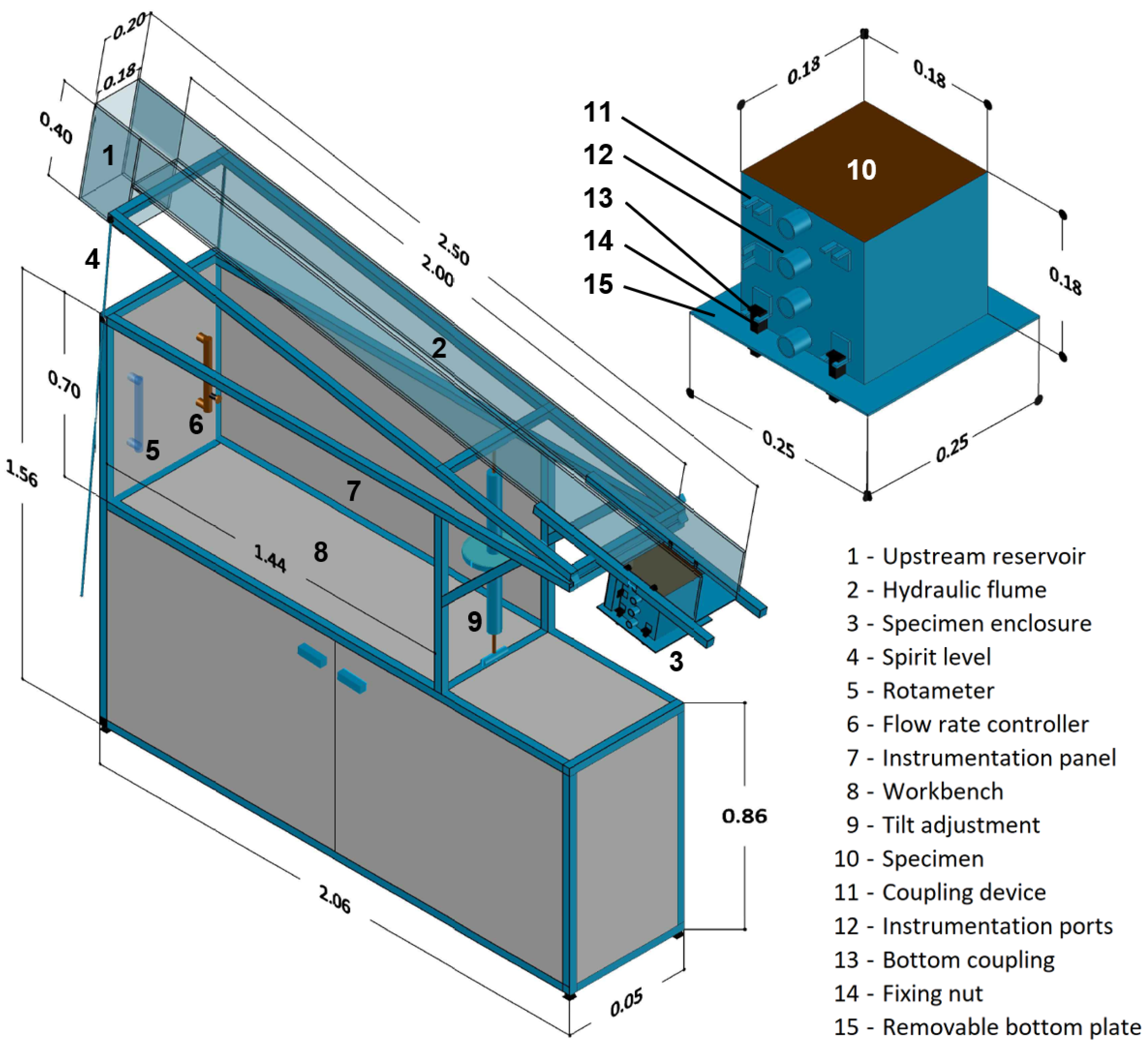
2.1. General Apparatus Characteristics and Hydraulic Design

The general arrangement of the developed apparatus is presented in Figure 2. It consists of (a) a reservoir made of polymethyl methacrylate, which can be used to regulate the water flow; (b) a flume made of the same material; (c) systems for regulating the flow and leveling the flume; and (d) a sample port. The system has a ramp length of 2.0 m, a base width of 0.18 m, and sidewalls that are 0.20 m in height. These dimensions were defined according to a flow analysis that will be described later on. The specimen enclosure is cubic and has edges of 18.0 cm in length. Ports were included in the specimen enclosure and were placed along uniformly spaced positions in the direction orthogonal to the specimen surface, allowing the instrumentation of the specimen using tensiometers and/or water content probes. The flume was designed to operate with tilt angles varying between 5 and 60 degrees. The design flow rates vary between 1.0 × 10⁻⁴ m³ s⁻¹ and 2.4 × 10⁻³ m³ s⁻¹ when the flume is set with a tilt angle of 5 degrees and between 4.0 × 10⁻⁴ m³ s⁻¹ and 9.0 × 10⁻³ m³ s⁻¹ in the maximum slope of 60 degrees.

As a design requirement, it was established that the apparatus should ensure a uniform flow condition in a supercritical regime over the specimen surface. A uniform flow corresponds to a constant flow velocity at any instant and at every point along the flume, including the specimen area. This design condition has been generally overlooked in previous open channel flume designs. A supercritical regime would allow the reproduction of uniform and controlled hydraulic shear stresses along the specimen surface [44]. In addition, flow disturbance that may occur in the downstream portions of the specimen as the erosion process advances would not propagate to upstream regions, keeping the flow characteristics relatively uniform.

In previous studies, it was assumed that the critical flow depth was equal to the normal depth along the flume, corresponding to a constant uniform flow under a critical regime. However, feeding the canal in a typical flume causes a phenomenon known as hydraulic backwater, resulting in a non-uniform flow regime at the entrance point of the flume. According to Munson et al. [44], this flow regime tends to evolve rapidly towards a permanent and non-uniform flow in a critical regime, in which the normal flow height is affected, compromising the strict control of hydraulic shear stresses.

The normal flow height value in the uniform flow region can be obtained using explicit solutions for trapezoidal channels, as presented in Vatankhah [45]. Taking the difference between the discharge in the uniform flow region and the feed discharge (Q), which depends on the flow height itself, the following equation is obtained:

$$f(y_0)=\frac{1}{n}\frac{{\left(b{y}_0\right)}^{5/3}{(\sin \alpha )}^{1/2}}{{(b+2y_0)}^{2/3}}-Q$$

(3)

where $f\left(y_0\right)$ is the tolerance for discharge variation; $n$ is Manning’s roughness coefficient (assumed to be 0.085 for polymethyl methacrylate); b is the flume width (m); $y_0$ is the flow depth, taken normal to the flume bed (m); $\alpha$ is the tilt slope of the flume; and $Q$ is the system discharge (m³ s⁻¹).

Equation (3) is a non-linear and indeterminate equation. The value of $y_0$ can be obtained iteratively, using Newton’s method, as follows:

$$y_{0_{(n+1)}}=y_{0_{(n)}}-\frac{f(y_{0_{(n)}})}{f^{\prime }(y_{0_{(n)}})}$$

(4)

where $y_0{}_{\left(i\right)}$ is the ith value of $y_0$, which is evaluated during the iterative procedure, and $f^{\prime }\left(y_0{}_{\left(i\right)}\right)$ is the first-order derivative of $f\left(y_0\right)$. The derivative estimation can be completed using the complex step approach method, described in Martins et al. [46]:

$$f^{\prime }(y_0)=\frac{\mathrm{Im}\left[f(y_0+ip)\right]}{p}$$

(5)

where Im is the image of the complex function, and p is the finite difference interval.

To guarantee uniform flow in a supercritical regime along the entire flume, including its entry and exit sections, the flow rate and the slope of the flume must be constrained by certain limits so that the hydraulic backwater dissipates before the specimen insertion region. Therefore, for each selected discharge, the distance between the starting point of the flow and the point where the normal height reaches the value of y₀ was calculated. It was thus possible to confirm the occurrence of the specified flow regime. Such evaluation was conducted for each selected discharge using the direct step numerical integration method as presented by Munson et al. [44].

2.2. Soil Characteristics and Specimen Preparation for Flume Tests

The soil selected for this study has characteristics that are typical of soils from the state of Goiás, Brazil. Disturbed samples were collected in the city of Goiânia at the geographical coordinates 16.7289° S and 49.2958° W. Samples were collected between 50 cm and 150 cm below the ground surface, reaching the B horizon. The soil has a clay content above 20%. The soil presents liquid and plastic limits of 33% and 22%, respectively, and a pH of 5.6, which is typical for lateritic soils from the region. The in situ void ratio varies from 1.0 to 1.8, and the saturated hydraulic conductivity ranges from 1 × 10⁻⁶ m s⁻¹ to 2 × 10⁻⁵ m s⁻¹. Finally, the soil has a cation exchange capacity of 2.29 cmol dm⁻³ and an amount of organic matter of 9 g dm⁻³.

Laboratory specimens were reconstituted under highly controlled conditions. A quasistatic compaction procedure was adopted, using the Emic DL2000 automated loading frame manufactured by Instron (Norwood, MA, USA). The specimen enclosure shown in Figure 2 was used as a mold. Specimen compaction was achieved using four soil layers of 50 mm in height each, each one compressed at a constant rate of 0.017 mm/s. A 50 mm extension collar was used to hold the loose soil before compression. After compaction, the collar was gently removed, exposing 20 mm of excess compacted material. Finally, the excess material was scraped using a beveled ruler so that the specimen would reach the final 180 mm in height. This scraping procedure ensured that the specimen surface roughness was not influenced by the compaction piston, which often produces undesired particle orientation. Specimens were sealed and stored to reach hydraulic equilibrium for at least two days before testing.

Specimens were reconstituted using air-dried samples that were later wetted to a gravimetric water content of 18%. The selected remolding void ratios were equal to 1.0 and 1.5. The mean value and coefficient of variation (CV) obtained for the gravimetric water content, considering all reconstituted specimens, was 17.8% and 0.4%, respectively. The mean value obtained for the void ratio of remolded specimens was 1.02 and 1.51. The corresponding values for CV of the void ratios were 0.6% and 0.4%, respectively. The obtained mean and CV values indicate that the compaction procedure was adequate, producing specimens that correspond closely to the specified conditions. It is important to note that the remolding process does not necessarily produce specimens with the same soil structure as the one found in natural undisturbed soil. However, flume test repeatability benefits greatly from the use of the relatively homogeneous specimens obtained from the compaction procedure.

2.3. Flume Testing Procedure

Before the execution of each test, the specimens were unsealed and weighed to confirm the remolding water content after the equilibrium period. The placement of the specimens in the flume was achieved to ensure the strict alignment between the specimen surface and the hydraulic flume. The relatively narrow gap (smaller than 1 mm) located along the edges of the specimen surface was sealed using silicone glue, removing excess glue, and leveling it. Next, the specimen surface was covered with a polyethylene plastic film. Water was allowed to flow over the covered specimen until the desired flow rate and flow regime uniformity was observed. The start of the test proper was established by carefully removing the protection film.

The eroded material was collected using sieves covered with non-woven polyester geotextile with a mass of 140 g m⁻² and an apparent opening equal to 0.094 mm, which was calculated based on the retention criteria presented by Christopher and Holtz [47]. The geotextile was oven-dried at approximately 104 °C for at least 24 h and were weighed on a precision scale before use in the test.

To investigate the evolution of erosion over time, from its initial seconds to prolonged periods of flow, the eroded material was collected after 0.25, 0.5, 1, 2, 3, 4, 5, 10, 15, 30, 45, and 60 min. The eroded mass between each time step was determined by placing a new sieve-geotextile set on top of the existing one and by removing the latter. Each sediment collection geotextile was placed in an oven that was set at approximately 105 °C for at least 24 h, and the geotextiles were then weighed to obtain the eroded dry soil mass.

2.4. Flume Testing Program

The experimental program presented herein involved a total of 31 specimens with hydraulic conditions that were selected to allow the determination of the erosion parameters established by the WEPP model framework. The test conditions were combined to produce the following sets:

• Out of the 31 specimens, a total of 16 specimens were compacted at a void ratio of 1.5. The remaining 15 specimens were compacted with a void ratio of 1.0;
• Out of the 31 specimens, 12 were used to assess the repeatability of the tests performed with the new apparatus. This was accomplished by testing six pairs of specimens under identical flow conditions;
• Five different flow conditions were used to analyze the influence of the hydraulic shear stress on the erosion curves.

Hydraulic stresses of 0.98 Pa, 1.26 Pa, and 1.93 Pa were applied to specimens with void ratios of 1.0. Hydraulic stresses of 0.82 Pa, 0.98 Pa, and 1.26 Pa were selected for specimens with void ratios of 1.5. To obtain the aforementioned hydraulic stresses, a 10-degree tilt was adopted and was combined with flow rates of 1.5 × 10⁻³ m³ s⁻¹, 2.0 × 10⁻³ m³ s⁻¹, 2.5 × 10⁻³ m³ s⁻¹, 3.0 × 10⁻³ m³ s⁻¹, and 6.0 × 10⁻³ m³ s⁻¹. These conditions were based on their recurrence in previous studies.

3. Results and Discussion

As shown in Figure 1b, flume tests executed under multiple hydraulic shear stresses, τ_h, are required to define pairs of values of τ_h and D_c, thereby allowing the determination of the soil erosion properties, τ_h and K_r. Unfortunately, the erosion rate, D_c, may vary during testing. This is particularly true when fixed specimens are employed because the erosion curves under these testing conditions often present a hyperbolic behavior. As a result, several authors recommend that D_c be defined using a secant to the soil loss curve [15]. The secant value of D_c is obviously dependent on the time interval that is adopted. However, there is a lack of consensus in the literature regarding the elapsed time to be used for the computation of a secant erosion rate. Such a relatively imprecise definition of D_c prompted an investigation of the effect of the time interval.

Figure 3 presents the results of 12 flume tests. Accumulated soil loss (E) curves are shown over time for three pairs of hydraulic shear stress values and for two void ratio values. The erosion curves obtained from the tests performed on the specimens with void ratio of 1.5 (Figure 3b) and under hydraulic shear stresses of 0.82 Pa and 1.26 Pa indicated superior repeatability during the beginning of the erosion process, particularly within the first five minutes of testing. On the other hand, curves for the same hydraulic stress diverge for times longer than five minutes. Erosion curves obtained for specimens prepared with a void ratio of 1.0 presented significantly higher variability, which indicates some degree of randomness, even during the first five minutes. This fact can be explained by the low erodibility of the specimen surface with eroded material that is likely to only corresponded to the loosened soil particles present on the specimen surface before the test started.

The data presented in Figure 3 were modelled using a nonlinear fitting procedure aimed at defining the initial rate of soil loss and the maximum accumulate erosion value in a rigorous unbiased manner. The soil loss accumulated over time has a behavior that may be approximated by a hyperbolic function, as is apparent from Figure 3. The hyperbolic behavior may be mathematically represented as follows:

$$E=\frac{t}{\frac{1}{E_{ult}}t+\frac{1}{a_0}}$$

(6)

where $E$ is the soil loss by unit area accumulated at any given elapsed time (g cm⁻²); t is the elapsed time (min); $E_{ult}$ is the maximum asymptotic value of E, which is somewhat similar to the main erosion parameter defined in [15,42,48]; and $a_0$ is a fitting parameter (g cm⁻² min⁻¹).

The fitting parameter $a_0$ is the rate of erosion taken at the origin of the erosion curve and may be considered as the erosion rate defined in the WEPP model [5], $D_c$:

$${\frac{dE}{dt}|}_{\Delta t\to 0}=a_0=D_c$$

(7)

Nonlinear regression was conducted for the data presented in Figure 3 and only considered the first five minutes of testing. The analysis time was limited to the first five minutes because of the random nature of the erosion curves at later stages.

Table 1. Results of nonlinear regression modelling using the hyperbolic equation.

Void Ratio	Test	τh (Pa)	Dc(×10−2) (g cm−2 mim−1)	${\mathit{E}}_{\mathit{u}\mathit{l}\mathit{t}}(\times 10{-}^2)$ (g cm−2)	RMSE (×10−4)	R2
1.000	1	0.98	0.81	0.14	0.73	0.931
	2	0.98	1.25	0.60	2.52	0.950
	3	1.26	1.00	0.70	4.46	0.940
	4	1.26	2.85	0.62	0.66	0.937
	5	1.93	4.03	0.35	1.14	0.972
	6	1.93	5.55	0.55	1.20	0.984
1.500	7	0.82	0.89	2.01	6.27	0.993
	8	0.82	0.52	0.97	8.78	0.912
	9	0.98	0.83	1.48	9.24	0.942
	10	0.98	4.00	5.43	15.9	0.999
	11	1.26	2.85	5.54	12.5	0.998
	12	1.26	2.20	4.65	17.6	0.997

presents the results of the regression analysis. The continuous curves shown in Figure 3 present the corresponding best-fit curves. The results shown in Table 1 indicate RMSE values that range between 0.66 × 10⁻⁴ and 17.6 × 10⁻⁴ and R² values that range between 0.912 and 0.999. The quality of the fitting results was considered adequate for the purposes of this analysis.

The values of $D_c$ shown in Table 1 present a clear increasing trend for larger values of hydraulic shear stress, ${\tau }_h$. The relationship between ${\tau }_h$ and $E_{ult}$, however, did not indicate a clear positive correlation for tests 1–6. Some variability is observed in the repeatability analyses comparing the values of tests under the same shear stress. The relative difference of $D_c$ between identical tests ranged between 30% and 380%. The relative difference of $E_{ult}$ between identical tests range between 13% and 326%. The higher relative differences can be partially attributed to the fact that the mass loss of specimens compacted with void ratios of 1.0 was relatively low and only corresponded to loosened soil particles. Unfortunately, previous studies using open channels and fixed specimens have not presented similar systematic evaluations of repeatability that could be compared to those presented herein.

Figure 4a,b show the variation of ${\tau }_c$ and $K_r$ as a function of the adopted analysis time interval for the tests conducted with a void ratio of 1.5. There is some variation in the values of ${\tau }_c$ and $K_r$ according to the adopted time interval, and the values of ${\tau }_c$ reach a constant value after 5 min. Thus, while simultaneously meeting the requirements of repeatability and stabilization of erosion parameters, the analysis time of 5 min is recommended for the soil studied here. The typical behavior of the mass loss curves in the flume trials [41,48] indicate that the analysis time selection criterion proposed here has the potential to be applied to other soils.

The criterion for establishing the ideal analysis time seems to be related to the transition between an initial test stage in which erosion occurs uniformly along the specimen surface and a later stage in which cavities start to be randomly formed on the soil surface, as shown in Figure 5. The random character of the formation of the cavities and the loss of uniformity of the hydraulic conditions on the surface of the specimens indicate that the time interval representative of the flume test must be delimited for each soil based on the examination of the accumulated mass loss curve over time. Such an ideal time interval would correspond to the initial erosion stage, which can be identified as an approximately linear relationship between accumulated erosion and time. The curve transition and the maximum mass loss tend to have a random character that depends on the manner in which the specimen surface develops grooves and cavities.

The lateritic soil studied herein presented a ${\tau }_c$ from 0.69 to 0.78 Pa and a $K_r$ from 0.0014 to 0.012 g cm⁻² min⁻¹ Pa⁻¹. The values of ${\tau }_c$ and $K_r$ for the lateritic soils vary greatly and depend on the soil texture, soil weathering, and stability of particle aggregations. Some of the values of ${\tau }_c$ reported in the literature for lateritic soils range between 0.01 and 1.33 Pa [15,41,49]. The range of K_r for the lateritic soils reported by the same authors varies between 0.01 and 36.5 g cm⁻² min⁻¹ Pa⁻¹ [15,41,49]. Therefore, the results presented in Figure 4 fall within these typical ranges but also indicate that the soil studied herein has a relatively low erodibility when considering the values for other lateritic soils.

4. Final Remarks

The apparatus presented herein met the established requirements, allowing the control of imposed hydraulic conditions, which were defined by the flume’s slope and flow rate. The effluent collection method proved to be adequate, allowing the evaluation of the erodibility and of the conditions of the specimen during the test. The use of uniform flow in a supercritical regime allowed the strict control of the water flow height and of the hydraulic shear stresses that were imposed. In this sense, the cost-effective design characteristics of the apparatus (i.e., the use of an open channel and of a fixed specimen) proved to be a viable alternative for studying the erosion characteristics of soils subjected to water flow.

It was possible to perceive a relatively low test repeatability when comparing the results for identical conditions. However, this variability is expected given the complex nature of water erosion processes in soils. Further studies are recommended regarding ideal testing methodologies that would ensure improvements in test result repeatability. Future comparisons of the test results obtained using fixed and moving specimens (i.e., extruded at a speed defined by the erosion rate) would be of great value.

The results from the experimental program presented herein indicate that the slope of the initial stage of the mass loss curve give more consistent results when compared against the final maximum mass loss. Thus, it is proposed that only the initial section of the mass loss curves be considered during the analysis of erosion tests. The interpretation of the mass loss curves must also consider the observation of the physical characteristics of the specimen surface since the randomness of the maximum mass loss value can be attributed to the cavities that form after the linear rate erosion phase. Finally, the definition of the erodibility parameters of the WEPP methodology must consider time intervals that are within the initial erosion phase and that correspond to the linear portion of the mass loss curves.

This study was specifically focused on establishing adequate techniques for the evaluation of soil erodibility parameters. In this sense, the determination of representative field hydraulic conditions is of paramount importance for the adequate planning and specification of flume testing parameters. The hydraulic shear stresses and corresponding flow velocities selected for soil testing must be based on expected field values, which may be obtained based on an adequate hydrological model [50].

Finally, it is important to note that field testing devices and approaches based on the monitoring of field plots offer important alternatives for the assessment of soil erosion, in particular for bioengineering studies, the evaluation of the effect of vegetation, and the study of soil management practices [51,52]. Field testing also offers unique alternatives for considering real atmospheric events, including realistic rainfall patterns [53], which are difficult to reproduce under laboratory conditions [54,55]. Improving laboratory techniques, such as the device presented herein, allows inexpensive and relatively fast evaluations of soil erosion. However, the use of small-scale laboratory apparatuses and techniques have not been widely employed in the study for the effect of vegetation and bioengineering applications, and further studies are welcomed.

References

1. Julian, J.P.; Torres, R. Hydraulic Erosion of Cohesive Riverbanks. Geomorphology 2006, 76, 193–206. [Google Scholar] [CrossRef]
2. Meng, X.M.; Jia, Y.G.; Shan, H.X.; Yang, Z.N.; Zheng, J.W. An Experimental Study on Erodibility of Intertidal Sediments in the Yellow River Delta. Int. J. Sediment Res. 2012, 27, 240–249. [Google Scholar] [CrossRef]
3. Rinaldi, M.; Mengoni, B.; Luppi, L.; Darby, S.E.; Mosselman, E. Numerical Simulation of Hydrodynamics and Bank Erosion in a River Bend. Water Resour. Res. 2008, 44. [Google Scholar] [CrossRef] [Green Version]
4. Kimiaghalam, N.; Goharrokhi, M.; Clark, S.P.; Ahmari, H. A Comprehensive Fluvial Geomorphology Study of Riverbank Erosion on the Red River in Winnipeg, Manitoba, Canada. J. Hydrol. 2015, 529, 1488–1498. [Google Scholar] [CrossRef]
5. Foster, G.R. Modeling the Erosion Process. In Hydrologic Modeling of Small Watersheds, 1st ed.; Haan, C.T., Johnson, H.P., Brakensiek, D.L., Eds.; American Society of Agricultural Engineers: St. Joseph, MI, USA, 1982; pp. 297–380. [Google Scholar]
6. Baigorria, G.A.; Romero, C.C. Assessment of Erosion Hotspots in a Watershed: Integrating the WEPP Model and GIS in a Case Study in the Peruvian Andes. Environ. Model. Softw. 2007, 22, 1175–1183. [Google Scholar] [CrossRef]
7. Pandey, A.; Chowdary, V.M.; Mal, B.C.; Billib, M. Runoff and Sediment Yield Modeling from a Small Agricultural Watershed in India Using the WEPP Model. J. Hydrol. 2008, 348, 305–319. [Google Scholar] [CrossRef]
8. Dey, S. Fluvial Hydrodynamics—Hydrodynamic and Sediment Transport Phenomena, 1st ed.; Springer: Berlin/Heidelberg, Germany, 2014; 687p. [Google Scholar]
9. Shen, N.; Wang, Z.; Wang, S. Flume Experiment to Verify WEPP Rill Erosion Equation Performances Using Loess Material. J. Soils Sediments 2016, 16, 2275–2285. [Google Scholar] [CrossRef]
10. Pandey, A.; Himanshu, S.K.; Mishra, S.K.; Singh, V.P. Physically Based Soil Erosion and Sediment Yield Models Revisited. Catena 2016, 147, 595–620. [Google Scholar] [CrossRef]
11. Du Boys, M.P. Le rhone et les rivieres a lit affouillable. Ann. Ponts Chaussés 1879, 18, 141–195. [Google Scholar]
12. Partheniades, E. Erosion and deposition of cohesive soils. J. Hydraul. Hydraul. Eng. 1965, 91, 105–138. [Google Scholar]
13. Nearing, M.A.; Deer-Ascough, L.; Laflen, J.M. Sensitivity Analysis of the WEPP Hillslope Profile Erosion Model. Trans. ASAE 1990, 33, 839–849. [Google Scholar] [CrossRef]
14. Zhang, X.C.; Nearing, M.A.; Risse, L.M.; McGregor, K.C. Evaluation of WEPP Runoff and Soil Loss Predictions Using Natural Runoff Plot Data. Trans. ASAE 1996, 39, 855–863. [Google Scholar] [CrossRef]
15. Bastos, C.A.B. Estudo Geotécnico Sobre a Erodibilidade de Solos Residuais não Saturados. Ph.D. Thesis, Universidade Federal do Rio Grande do Sul, Porto Alegre, Brazil, 1999. [Google Scholar]
16. Kimiaghalam, N.; Clark, S.P.; Ahmari, H. An Experimental Study on the Effects of Physical, Mechanical, and Electrochemical Properties of Natural Cohesive Soils on Critical Shear Stress and Erosion Rate. Int. J. Sediment Res. 2016, 31, 1–15. [Google Scholar] [CrossRef]
17. Nearing, M.A.; West, L.T.; Brown, L.C. A Consolidation Model for Estimating Changes in Rill Erodibility. Trans. ASAE 1988, 31, 0696–0700. [Google Scholar] [CrossRef]
18. Sanford, L.P.; Maa, J.P.Y. A Unified Erosion Formulation for Fine Sediments. Mar. Geol. 2001, 179, 9–23. [Google Scholar] [CrossRef]
19. Khanal, A.; Klavon, K.R.; Fox, G.A.; Daly, E.R. Comparison of Linear and Nonlinear Models for Cohesive Sediment Detachment: Rill Erosion, Hole Erosion Test, and Streambank Erosion Studies. J. Hydraul. Eng. 2016, 142, 04016026. [Google Scholar] [CrossRef]
20. Wardinski, K.M.; Guertault, L.; Fox, G.A.; Castro-Bolinaga, C.F. Suitability of a Linear Model for Predicting Cohesive Soil Detachment during Jet Erosion Tests. J. Hydrol. Eng. 2018, 23, 06018004. [Google Scholar] [CrossRef]
21. Gao, X.; Wang, Q.; Ma, G. Experimental Investigation on the Erosion Threshold and Rate of Gravel and Silty Clay Mixtures. Trans. ASABE 2019, 62, 867–875. [Google Scholar] [CrossRef]
22. Khanal, A.; Fox, G.A.; Guertault, L. Soil Moisture Impacts Linear and Nonlinear Erodibility Parameters from Jet Erosion Tests. Trans. ASABE 2020, 63, 1123–1131. [Google Scholar] [CrossRef]
23. Lane, L.J.; Foster, G.R.; Nicks, A.D. Use of fundamental erosion mechanics in erosion prediction. Am. Soc. Agric. Eng. 1987, 11. Available online: https://agris.fao.org/agris-search/search.do?recordID=US8843443 (accessed on 20 September 2021).
24. Lim, S.S.; Khalili, N. An improved rotating cylinder test design for laboratory measurement of erosion in clayey soils. Geotech. Test. J. 2018, 32, 1–7. [Google Scholar] [CrossRef]
25. Lyle, W.M.; Smerdon, E.T. Relation of Compaction and Other Soil Properties to Erosion Resistance of Soils. Trans. ASAE 1965, 8, 419–422. [Google Scholar] [CrossRef]
26. Zhang, H.Y.; Li, M.; Wells, R.R.; Liu, Q.J. Effect of Soil Water Content on Soil Detachment Capacity for Coarse- and Fine-Grained Soils. Soil Sci. Soc. Am. J. 2019, 83, 697–706. [Google Scholar] [CrossRef] [Green Version]
27. Nearing, M.A.; Parker, S.C. Detachment of Soil by Flowing Water Under Turbulent and Laminar Conditions. Soil Sci. Soc. Am. J. 1994, 58, 1612. [Google Scholar] [CrossRef]
28. Debnath, K.; Nikora, V.; Aberle, J.; Westrich, B.; Muste, M. Erosion of Cohesive Sediments: Resuspension, Bed Load, and Erosion Patterns from Field Experiments. J. Hydraul. Eng. 2007, 133, 508–520. [Google Scholar] [CrossRef]
29. Tolhurst, T.J.; Black, K.S.; Paterson, D.M.; Mitchener, H.J.; Termaat, G.R.; Shayler, S.A. A Comparison and Measurement Standardisation of Four in Situ Devices for Determining the Erosion Shear Stress of Intertidal Sediments. Cont. Shelf Res. 2000, 20, 1397–1418. [Google Scholar] [CrossRef]
30. Ghebreiyessus, Y.T.; Gantzer, C.J.; Alberts, E.E.; Lentz, R.W. Soil Erosion by Concentrated Flow: Shear Stress and Bulk Density. Trans. ASAE 1994, 37, 1791–1797. [Google Scholar] [CrossRef]
31. Kamphuis, J.W.; Gaskin, P.N.; Hoogendoorn, E. Erosion Tests on Four Intact Ontario Clays. Can. Geotech. J. 1990, 27, 692–696. [Google Scholar] [CrossRef]
32. Zhu, J.C.; Gantzer, C.J.; Peyton, R.L.; Alberts, E.E.; Anderson, S.H. Simulated Small-Channel Bed Scour and Head Cut Erosion Rates Compared. Soil Sci. Soc. Am. J. 1995, 59, 211–218. [Google Scholar] [CrossRef]
33. Cantalice, J.R.B.; Cassol, E.A.; Reichert, J.M.; Borges, A.L.O. Hidráulica do escoamento e transporte de sedimentos em sulcos em solo franco-argilo-arenoso. Rev. Bras. Ciênc. Solo 2005, 29, 597–607. [Google Scholar] [CrossRef]
34. Shepard, D.M.; Bloomquist, D.; Henderson, M.; Kerr, K.; Trammell, M.; Marin, J.; Slagle, P. Design and Construction of Apparatus for Measuring Rate of Water Erosion of Sediments, 1st ed.; The National Academies of Science, Engineering, Medicine: Washington, DC, USA, 2005; 66p. [Google Scholar]
35. Ni, S.; Zhang, D.; Wen, H.; Cai, C.; Wilson, G.V.; Wang, J. Erosion Processes and Features for a Coarse-Textured Soil with Different Horizons: A Laboratory Simulation. J. Soils Sediments 2020, 20, 2997–3012. [Google Scholar] [CrossRef]
36. Smerdon, E.T.; Beasley, R.P. Critical Tractive Forces in Cohesive Soils. J. Agric. Eng. 1961, 42, 26–29. [Google Scholar]
37. Shaikh, A.; Abt, S.R. Erosion Rate of Compacted NA-Montmorillonite Soils. J. Geotech. Eng. 1998, 114, 10. [Google Scholar] [CrossRef]
38. Ting, F.C.K.; Briaud, J.-L.; Chen, H.C.; Gudavalli, R.; Perugu, S.; Wei, G. Flume Tests for Scour in Clay at Circular Piers. J. Hydraul. Eng. 2001, 127, 969–978. [Google Scholar] [CrossRef]
39. Ravisangar, V.; Dennett, K.E.; Sturm, T.W.; Amirtharajah, A. Effect of Sediment PH on Resuspension of Kaolinite Sediments. J. Environ. Eng. 2001, 127, 531–538. [Google Scholar] [CrossRef]
40. Barry, K.M.; Thieke, R.J.; Mehta, A.J. Quasi-Hydrodynamic Lubrication Effect of Clay Particles on Sand Grain Erosion. Estuar. Coast. Shelf Sci. 2006, 67, 161–169. [Google Scholar] [CrossRef]
41. Koetz, M.; Pruski, F.F.; Mehl, H.U.; Silva, D.D.; Marques, E.A.G. Métodos Para a Determinação da Erodibilidade e da Tensão Crítica de Cisalhamento do Solo em Estradas não Pavimentadas. Rev. Eng. Agric. 2009, 17, 110–119. [Google Scholar] [CrossRef]
42. Almeida, J.G.R.; Romão, P.A.; Mascarenha, M.M.A.; Sales, M.M. Erodibilidade de solos tropicais não saturados nos municípios de Senador Canedo e Bonfinópolis (GO). Geociências 2015, 34, 441–451. [Google Scholar]
43. Wang, Y.-C.; Sturm, T.W. Effects of Physical Properties on Erosional and Yield Strengths of Fine-Grained Sediments. J. Hydraul. Eng. 2016, 142, 04016049. [Google Scholar] [CrossRef]
44. Munson, B.R.; Rothmayer, A.P.; Okiishi, T.H.; Huebsch, W.W. Fundamentals of Fluid Mechanics, 7th ed.; Wiley: Hoboken, NJ, USA, 2012; p. 792. [Google Scholar]
45. Vatankhah, A.R. Explicit Solutions for Critical and Normal Depths in Trapezoidal and Parabolic Open Channels. Ain Shams Eng. J. 2013, 4, 17–23. [Google Scholar] [CrossRef] [Green Version]
46. Martins, J.R.R.A.; Sturdza, P.; Alonso, J.J. The Complex-Step Derivative Approximation. ACM Trans. Math. Softw. 2003, 29, 245–262. [Google Scholar] [CrossRef] [Green Version]
47. Christopher, B.R.; Holtz, R.D. Geotextile Engineering Manual—Report FHWA-TS-86/203, 1st ed.; The National Academies of Science, Engineering, Medicine: Washington, DC, USA, 1985; p. 1044. [Google Scholar]
48. Nascimento, R.O.; Oliveira, L.M.; Mascarenha, M.M.A.; Angelim, R.R.; Oliveira, R.B.; Sales, M.M.; Luz, M.P. Uso de solução de cal para mitigação de processos erosivos em um solo da UHE de Itumbiara. Geociências 2019, 38, 279–295. [Google Scholar] [CrossRef]
49. Basso, L. Estudo da Erodibilidade de Solos e Rochas Sedimentares de Uma Voçoroca na Cidade de São Francisco de Assis—RS. Master’s Thesis, Universidade Federal de Santa Maria, Santa Maria, Brazil, 2013. (In Portuguese). [Google Scholar]
50. Grimaldi, S.; Nardi, F.; Piscopia, R.; Petroselli, A.; Apollonio, C. Continuous Hydrologic Modelling for Design Simulation in Small and Ungauged Basins: A Step Forward and Some Tests for its Practical Use. J. Hydrol. 2021, 595, 125664. [Google Scholar] [CrossRef]
51. Apollonio, C.; Petroselli, A.; Tauro, F.; Cecconi, M.; Biscarini, C.; Zarotti, C.; Grimaldi, S. Hillslope Erosion Mitigation: An Experimental Proof of a Nature-Based Solution. Sustainability 2021, 13, 6058. [Google Scholar] [CrossRef]
52. Stanchi, S.; Zecca, O.; Hudek, C.; Pintaldi, E.; Viglietti, D.; D’Amico, M.E.; Colombo, N.; Goslino, D.; Letey, M.; Freppaz, M. Effect of Soil Management on Erosion in Mountain Vineyards (N-W Italy). Sustainability 2021, 13, 1991. [Google Scholar] [CrossRef]
53. Mohamadi, M.A.; Kavian, A. Effects of Rainfall Patterns on Runoff and Soil Erosion in Field Plots. Int. Soil Water Conserv. Res. 2015, 3, 273–281. [Google Scholar] [CrossRef] [Green Version]
54. Mendes, T.A.; Pereira, S.A.d.S.; Rebolledo, J.F.R.; Gitirana, G.d.F.N., Jr.; Melo, M.T.d.S.; Luz, M.P.d. Development of a Rainfall and Runoff Simulator for Performing Hydrological and Geotechnical Tests. Sustainability 2021, 13, 3060. [Google Scholar] [CrossRef]
55. Mendes, T.A.; Alves, R.D.; Gitirana, G.d.F.N., Jr.; Pereira, S.A.d.S.; Rebolledo, J.F.R.; da Luz, M.P. Evaluation of Rainfall Interception by Vegetation Using a Rainfall Simulator. Sustainability 2021, 13, 5082. [Google Scholar] [CrossRef]
Figure 1. Erosion formation: (a) hydraulic conditions; (b) erosion function.
Water 13 02956 g001
Figure 2. Flume apparatus; all dimensions are in meters.
Water 13 02956 g002
Figure 3. Flume test results for void ratios of: (a) 1.0; (b) 1.5; (c) 1.0 modelled curves; and (d) 1.5 modelled curves. Filled and empty markers of the same shape indicate test pairs that were conducted under identical conditions.
Water 13 02956 g003aWater 13 02956 g003b
Figure 4. Evaluation of the time interval effect adopted in the definition of the parameters of the WEPP methodology (w0 = 18%, e = 1.5): (a) τ c ; (b) K r .
Water 13 02956 g004
Figure 5. Specimen surface condition after flume tests for various void ratios and hydraulic shear stresses: (a) test #5, at e = 1.0 and τ h = 1.93 Pa; (b) test #6, at e = 1.0 and τ h = 1.93 Pa; (c) test #7, at e = 1.5 and τ h = 0.82 Pa; and (d) test #8, at e = 1.5 and τ h = 0.82 Pa.
Water 13 02956 g005