
Flood Hazards in Flat Coastal Areas of the Eastern Iberian Peninsula: A Case Study in Oliva (Valencia, Spain)
by
 , and
, and
Miguel Ángel Eguibar
1,* ,
,
Raimon Porta-García
2,
Francisco Javier Torrijo
3,4 and
Julio Garzón-Roca
5 1
Institute for Water and Environmental Engineering (IIAMA), Department of Hydraulic Engineering and Environment, Universitat Politècnica de València, 46022 Valencia, Spain
2
Climate Change and Sustainable Development Sector (CSD), Division of Environment, Rural Development and Disaster Risk Management (RND), Inter-American Development Bank (IADB), Washington, DC 20577, USA
3
Research Centre PEGASO, Universitat Politècnica de València, 46022 Valencia, Spain
4
Department of Geological and Geotechnical Engineering, Universitat Politècnica de València, 46022 Valencia, Spain
5
Department of Geodynamics (GEODESPAL), Faculty of Geology, Complutense University of Madrid, 28040 Madrid, Spain
*
Author to whom correspondence should be addressed.
Water 2021, 13(21), 2975; https://doi.org/10.3390/w13212975
Submission received: 15 September 2021
/
Revised: 15 October 2021
/
Accepted: 19 October 2021
/
Published: 21 October 2021
(This article belongs to the Special Issue Research of River Flooding)
Abstract
:Enhancing resilience against flooding events is of great importance. Eastern Iberian Peninsula coastal areas are well known for high intensity rainfalls known as DANA or “cold drop”. Extreme records in 24 h can exceed the annual average of the historical series. This phenomenon occurs normally in autumn due to convective storms generated by the existence of cold air in the upper layers of the atmosphere combined with warm winds coming from the Mediterranean Sea. In many coastal areas of the Eastern Iberian Peninsula, their flat topography, sometimes of a marsh nature, and the natural (e.g., dune ridges) and man-made (e.g., infrastructures) factors, result in devastating flooding events of great potential damage and risk for urban and rural areas. In this context, this paper presents the case study of the town of Oliva (Valencia, Spain) and how in a flooding event the flow tends to spread and accumulate along the flat coastal strip of this populated area, causing great potential damage. From that point, the paper discusses the particular issues that flood studies should consider in such flat and heavy rainy areas in terms of the hydrological and hydraulic models to be conducted to serve as the key tool of a correct risk assessment. This includes the correct statistical simulation of rainfalls, the hydrological model dependency on the return period and the correct geometry definition of all possible water barriers. An analysis of the disturbance that climatic change effects may introduce in future flooding events is also performed.
1. Introduction
The Iberian Peninsula presents a particular climatic characterization. It is located between the North Atlantic region and the driest area of the subtropical high pressure belt [1,2]. The former is a humid-warm region regularly affected by storms associated with polar fronts. The latter provides high stability and scarcity of precipitations. The different regions belonging to the Iberian Peninsula are influenced during different times of the year by [3,4,5]: the wet fronts coming from the Atlantic Ocean; the dry air coming from the Sahara desert; the climatic stability given by its proximity to the Mediterranean Sea; and the polar fronts that eventually descend from the north of Europe. These phenomena cause great climatic variability between regions, and this is even associated with the character of the people who inhabit them. The mean annual rainfall for the historical series in Spain is 628 mm (Meteorological Agency of Spain-AEMET [6]), but the variance is very high. For instance, at Cabo de Gata (Almeria, SE Spain), rainfall barely reaches 150 mm/year, while in the town of Rois (La Coruña, NE Spain), its average is 2959 mm/year. Sudden alterations in the local climate can also be generated if rapid variations in the high- and low-pressure fronts occur.
Eastern Spanish regions are characterized by a relatively low average annual rainfall, barely exceeding 500 mm/year in Valencia and 420 mm/year in Alicante [6,7]. These low values are the result of three causes [8,9,10]: (i) the Iberian Peninsula Plateau has an average altitude of 800 m with various mountain systems crossing it, which gives rise to an orographic barrier to the waterfronts coming from the Atlantic Ocean (fronts are water unloaded when they arrive at the east of the Iberian Peninsula); (ii) the proximity to the Sahara desert, whose warm air masses are very stable and condition the free movement of the fronts to the south; and (iii) the blocking effect generated by the Azores anticyclone, very stable throughout the year, and which frequently represents a barrier to Atlantic storms.
However, during the last century, the East Spanish regions recorded the highest rainfalls in Europe. For example, on 19 October 2018, 159.2 mm were recorded between 18:00 and 19:00 at Vinarós (Castellón) and on 23 September 2008, 144.4 mm were recorded in just one hour at Sueca (Valencia). It should be noted that a very strong rain may be considered when the rain intensity is between 30 and 60 mm/h, while torrential rain exceeds 60 mm/h [11,12]. As these regions are semi-arid ones in which the vegetation cover is not abundant, the large amount of energy released by extreme rains generates significant erosion [13], worsening the rain effects on both natural and social areas. These rainfalls are convective precipitations, usually generated as a consequence of cold air pockets in the upper layers of the atmosphere and normally coming from the European continent, which are combined with east warm winds coming from the Mediterranean Sea [14,15,16,17]. Cold air pockets occur in the troposphere with temperatures between −25 and −30 °C, from 5 km above. This generates an accelerated forced condensation and clouds of great vertical development. The proximity of the Mediterranean Sea in these winds coming from the east feeds this generation of accelerated humidity/clouds in an almost uninterrupted way.
This phenomenon usually occurs in autumn (September to November) when the first cold fronts begin to descend from the North Pole towards the European continent, but the Mediterranean Sea is at a high temperature at that time as a result of summer. This mesoscale convective system is known as Isolated Depression at High Levels or DANA (after the Spanish expression “Depresión Aislada en Niveles Altos”). Colloquially, the phenomenon is known as “cold drop”. This weather circumstance supposes a great thermal shock, which generates storms of great intensity causing violent runoff with a great capacity for erosion and floods with a high destructive capacity [18]. Only one of these events could generate a rain discharge similar to the average historical annual rainfall [6,7,12]. Thus, the extreme rains in the East Spanish regions are characterized by their randomness and the high intensity that they can reach in a few days.
In addition, the geological and geomorphological features of the Eastern Iberian Peninsula result in having flat areas in the coastal regions. A coastal geomorphological structure combining flat areas of the Quaternary period crowned by mountainous elevations of the Tertiary period is typical and frequent on such regions of the Iberian Peninsula and the Spanish coasts. Great intensity rainfalls together with the existence of flat areas lead to regularly having important floods in those coastal regions [19]. Flood events cause potential damage to infrastructures, industries, homes, and people, thus requiring administrations to work on the development of flood risk management plans [20]. The basis of those plans is a flood study.
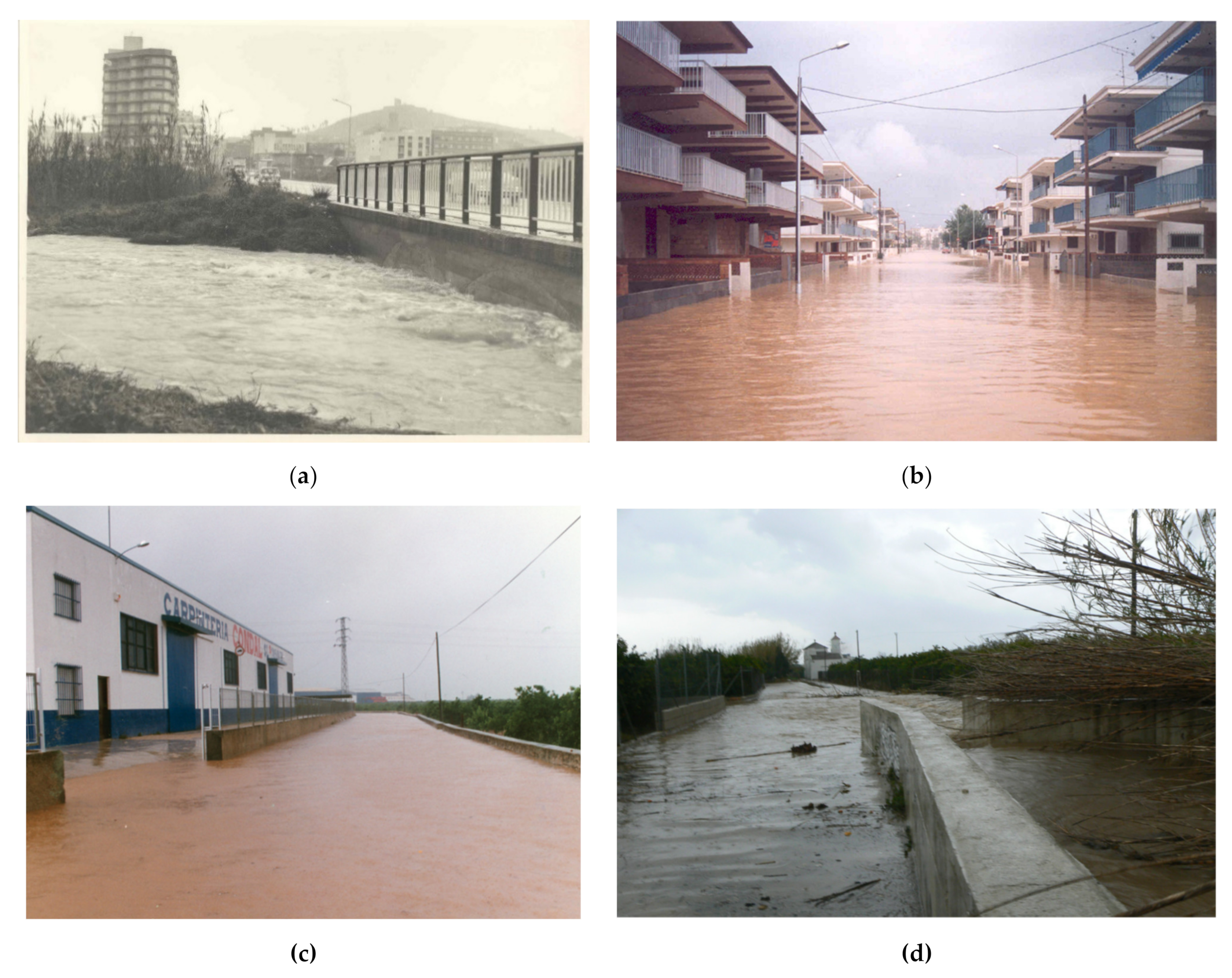
In this context, this paper aims at establishing how to properly address flood studies in flat coastal regions of the Eastern Iberian Peninsula. This is done through the analysis of a case study. The area under study corresponds to the surroundings of Oliva, a town with 25,200 inhabitants [21] located near the Mediterranean Sea and about 65 km to the south of Valencia. The area has a semi-arid climate and is characterized by an orography that facilitates sudden great rainfalls, so floods are common in the town: historical records show more than 20 extreme floods in the area since 1972. This means having an extreme flood every 2.5 years as average (although, in some years, more than one flooding event was recorded). The coastal area of Oliva is highly urbanized and flooding effects are dangerous due to the difficulties with which the water drains into the sea and the marsh nature of the area. In an extreme flood event, overflow flows uncontrollably through fields and roads, giving rise to great risk situations that can even cause life losses. Figure 1 shows some examples of those flood events in the area over the last 50 years.
Thus, the novelty of this work lies in establishing those special issues related to hydrological models and hydraulic simulations to be considered in flood studies in flat coastal areas belonging to the Eastern Iberian Peninsula. Some aspects dealt with in the paper include the correct statistical simulation of rainfalls, the hydrological model dependency on the return period and the correct geometry definition of all possible water barriers in the hydraulic model. Besides, some issues concerning climate change effects are also discussed in the paper due to its potential affection to sensitive flood parameters in the near future. Outcomes of this work are not exclusive of the Eastern Iberian Peninsula areas, but they can be extended to any region in the Western Mediterranean Sea coastal areas where flat surfaces and heavy rainfalls play an important role.
2. Materials and Methods
2.1. Geographical Setting and Geological Framework
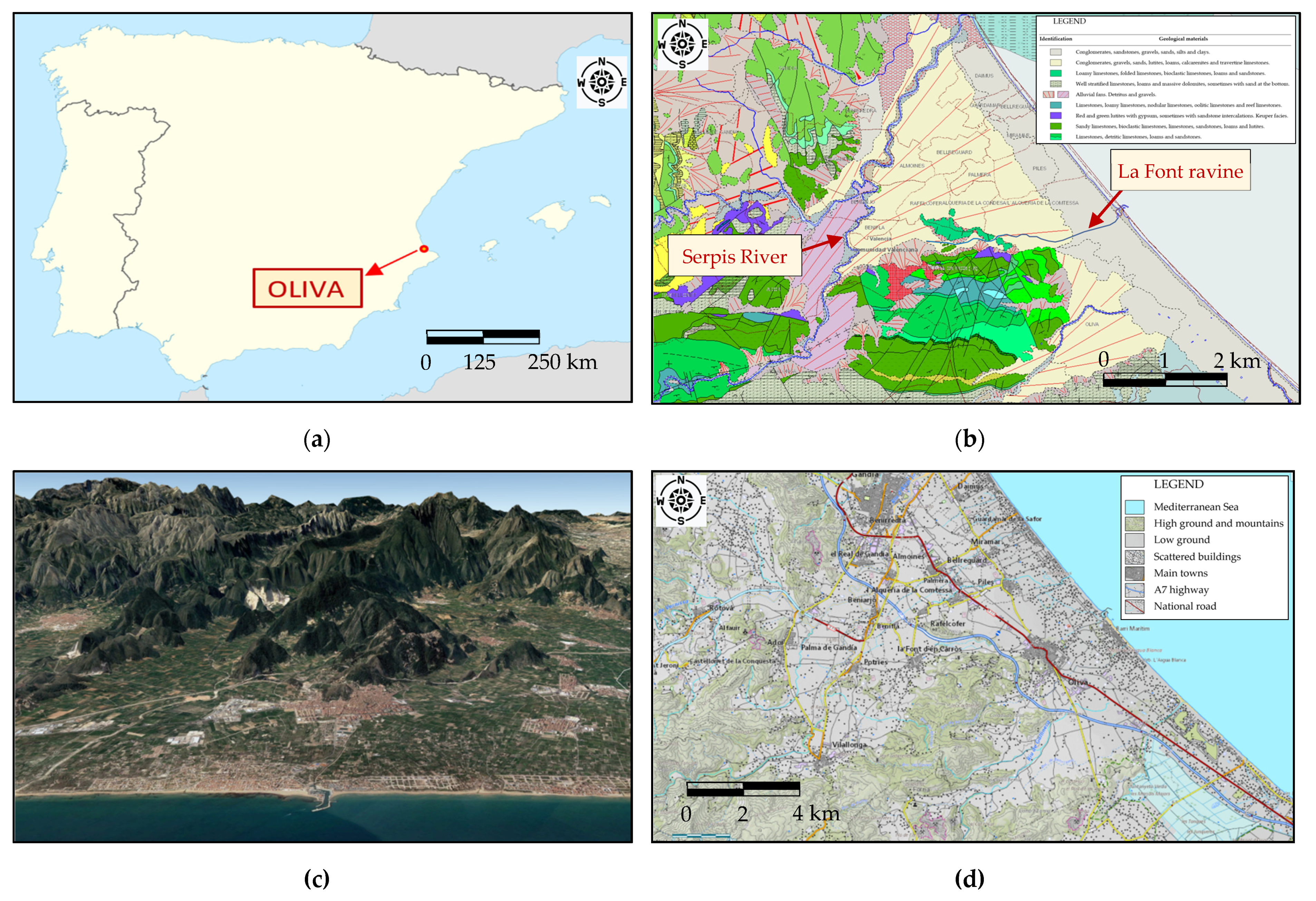
Figure 2a,b show the location of Oliva in the Iberian Peninsula and the geological framework of the area. The orography is characterized by the presence of mountains of a certain elevation close to the Mediterranean coast (Figure 2c). These mainly correspond to the last foothills of the Baetic System that run in the SW-NE direction through the south of the Iberian Peninsula, from the Algeciras Gulf to La Nao Cape. The latter is close to the area under study and there the Baetic System confluences with the Iberian System foothills (NW-SE direction) giving rise to rock masses of medium altitude, very fragmented by numerous faults and tectonic accidents. As a result, mountainous elevations in the area under study have a predominantly SW-NE direction in the vicinity of the coastal strip, although some influence of the Iberian System can also be seen in the area, with some mountain ranges following its direction, almost parallel to the coast. Materials are mainly Tertiary (Cretaceous and Jurassic), except in a wide strip close to the coast, where Quaternary deposits made up of recent materials can be found on a virtually flat surface, most of which correspond to terrains of a marsh nature.
The orographic factor has a decisive influence on local rainfalls [8,22]. When the rainy fronts advance from the sea towards the coast, the mountains generate a barrier that forces condensation and makes it difficult for the cloud masses to pass inland, discharging a large part of their water content abruptly. The confluence of a Mediterranean climate with episodes of significant torrential rains (cold drop or DANA), its effects increased by the existence of a mountainous range, barely parallel to the sea and close to it, cause the sudden discharge of precipitation with extreme intensity.
The area is crossed by various streams and ravines, with La Font ravine as the main way of natural runoff. The Serpis River is located towards the north of the area and its right bank alluvial fans force runoffs coming from La Font ravine to divert to the east. Besides, the Triassic dolomite outcrop found in the south of the area is a natural physical barrier for all flows. This means that the surface runoff tends to flow superficially in N-NE direction to the right bank of the Serpis River to avoid the rock outcrop. However, the special geomorphology of the Serpis River in its final section generates an adverse slope on its right bank. Consequently, the runoff tends to circulate superficially towards that river, but there is a natural redirection of flows from there towards the coast by the SE areas.
The abrupt interior orography forced for centuries the main human settlements and activity to develop, in general, on the flatter coastline. In addition, the communication routes that form the backbone of the Eastern Iberian Peninsula were developed along the coast. This results in a highly urbanized coastal area (Figure 2d), which is the receiver of a great amount of water that needs to be drained, but is where infrastructures and constructions create obstacles to surface runoff. Thus, the combination of all those factors leads to having important flooding events with a regular frequency affecting both rural and urban areas.
2.2. Flood Study
Flood studies are composed of two basic parts: first, a hydrological study is performed, based on climatic and territory analyses, to set the amount of water circulating in the territory and to obtain the peak flow values at key points; and secondly, a hydraulic study is carried out, using the data given by the hydrological study, to establish the depths reached by water at the different points of the territory as well as other data such as water velocities. Results are later used in flood plans and/or as the basis of any risk assessment study.
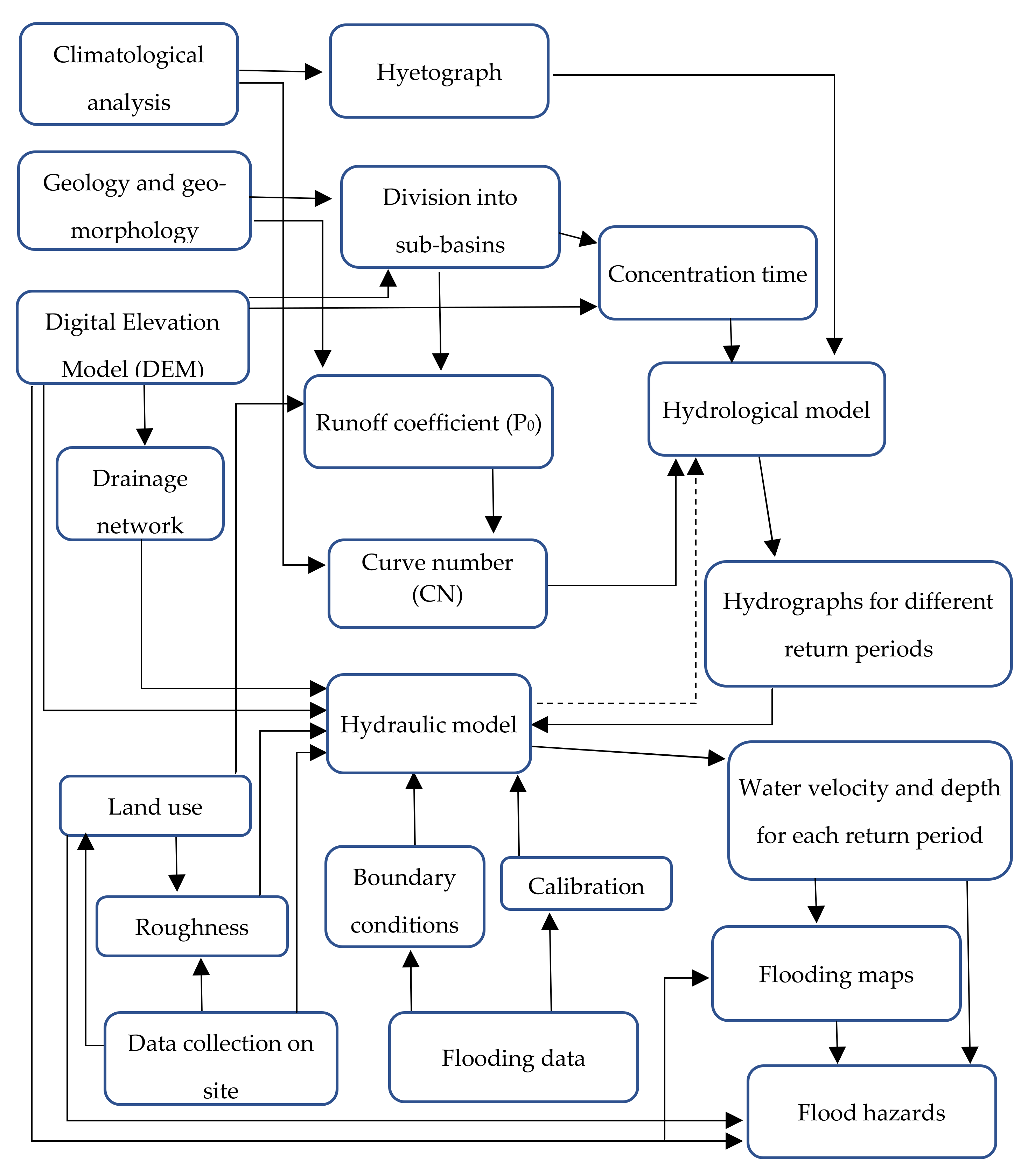
Figure 3 displays the methodological scheme followed in this paper, which is similar to the mentioned structure. This scheme can be divided into five blocks, four of which correspond to input blocks: territory analysis, climatic analysis, hydrological model, and hydraulic model. The fifth block corresponds to the output.
The following sections give details of each input block for its implementation in the present case study. It should be noted that the division into four input blocks does not mean each block to be independent, but some items are usually related to each other. For example, the hydrological model may depend on the results obtained by the hydraulic model, which in turn depends on the hydrological model itself (note that this is highlighted in Figure 3 by a dashed line). This generates a circular dependency that must be solved through an iterative process, something rarely considered in this kind of simulation, but which is essential when dealing with locations belonging to the type of geographical areas under study.
2.3. Territory Analysis
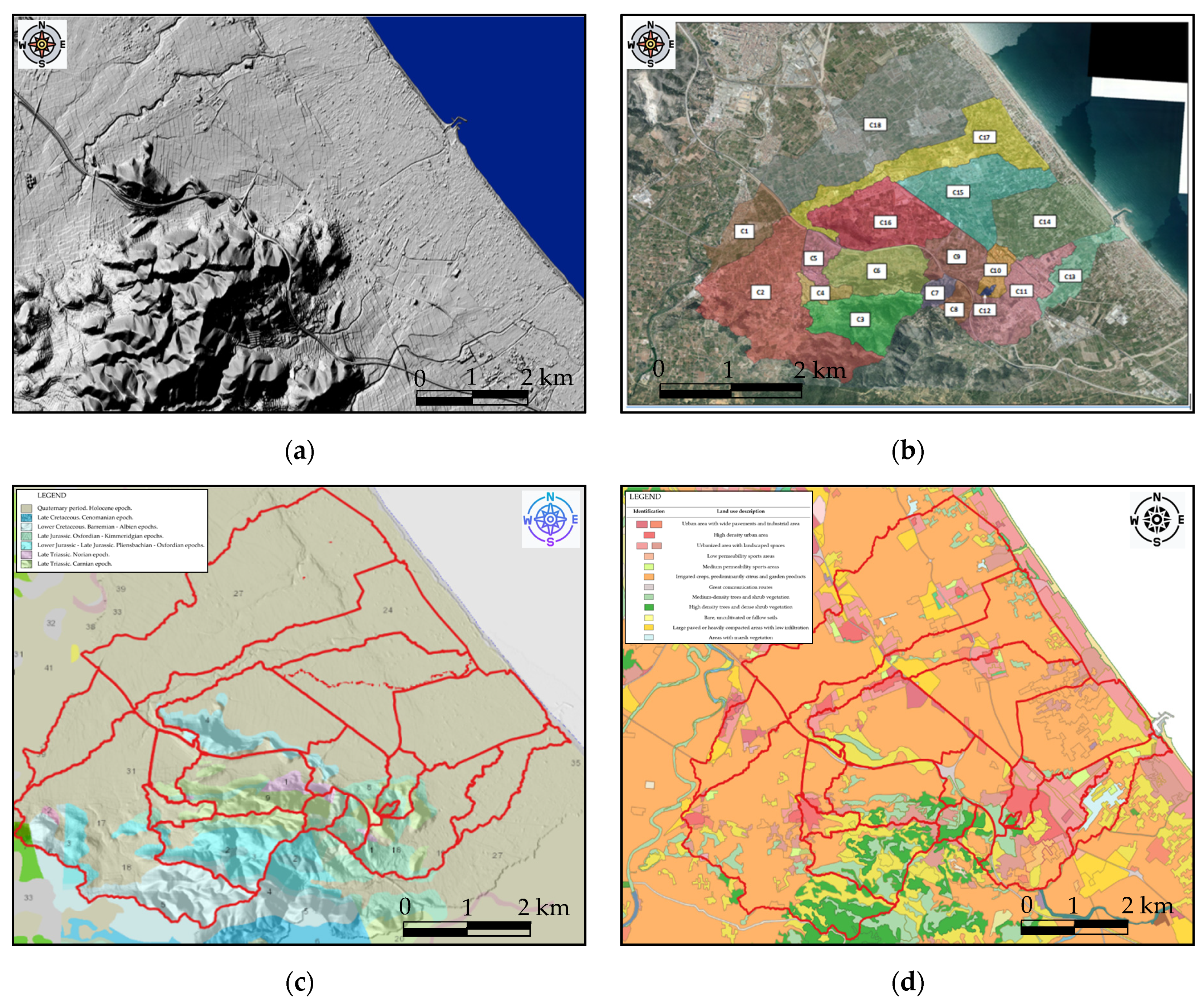
The PNOA’s cartographic database belonging to the Spanish National Geographic Institute [23] was used in this study. This contains high-precision digital elevation models (DEM) of Spain obtained by photogrammetric flight. Its updating period is 2–3 years. A specific DEM was prepared (Figure 4a) based on that cartographic database. The hydraulic connections in the area under study were manually introduced. Those elements (e.g., transverse drainage and bridges) are not recorded in the photogrammetric flights, but they are needed to properly develop the hydrological and hydraulic models. The hydrographical network of the area was established according to the elevations given in the DEM prepared. As Figure 4a shows, the flow networks draining towards the easterly direction start from the mountainous range located in the lower part of the image.
The total area of 38.9 km2 was divided into 18 sub-basins to reproduce the hydrological processes on a smaller scale, enabling evaluating the production and propagation of surface runoff. Figure 4b shows that division, while Table 1 gives the area of each sub-basin as well as the elevation of their centroids. The division was carried out considering topographic (slope) and hydrological (infiltration capacity) criteria, as well as the points in which measuring of flows was of interest. It should be noted that due to the proximity of the mountains to the sea, sub-basins generated at the flat coastal strip are small. Thus, although the perimeter of each sub-basin in the elevated areas is clear in topographic terms, division of the coastal strip was forced sometimes as it tends to generate a joint operation due to its marsh nature (e.g., C14 and C15 sub-basins present a joint operation in their lower section). Besides, some division followed existing highways, roads, and paths that generate barriers that condition the flow circulation in these flat and low level areas. This entire system could even be hydraulically connected for high return periods with overflowing flows on the right bank of the Serpis River. This is a problem that usually arises in this type of coastal areas, where sub-basin divisions may involve channels located out of the area under study.
Figure 4c shows the sub-basin overlapped with the geology and the orography. The infiltration capacity at each sub-basin was measured following the SCS (Soil Conservation Service) methodology [24]. Land uses and geology are the main factors controlling infiltration capacity. Land uses (Figure 4d) were established using the Spanish national records of SIOSE map [25] updated in 2017 and confirmed by visits to the area.
Land uses match to a certain extent the division between the Tertiary and Quaternary geological outcrops. In general, the land uses in the higher regions agree with areas of forest and scrubland (Tertiary), while at the lower regions, land uses agree with agriculture and urban areas prevail (Quaternary soils). From those data, the Curve Number (CN) at each sub-basin, needed to apply the SCS methodology, was obtained following the Spanish codes [26].
2.4. Climatic Analysis
Figure 5 shows the average precipitations per month in the area under study; data collected corresponds to a station located in the town of Oliva and the historical series range from 1940 to 2020 [6]. As can be observed, rainfall in the area is not abundant. The historical series presents an average annual record of 776 mm, with a dry summer period and a rainy period at the end of it. However, the local weather is strongly influenced by two factors: (i) the orography, with mountain ranges close to the coast whose orientation contributes to generating a barrier effect to the entry of water-laden fronts from the Mediterranean Sea; and (ii) the features of convective storms (DANA) generated in the Eastern Iberian Peninsula with very strong precipitation intensities and a displacement from East to West. The storm season occurs in autumn, after the summer period and when a thermal shock is likely to occur between the first cold fronts coming from the European continent and the warm waters of the Mediterranean Sea. Besides, the high temperature of the seawater after summer facilitates the generation of clouds of great vertical travel (convective storms).
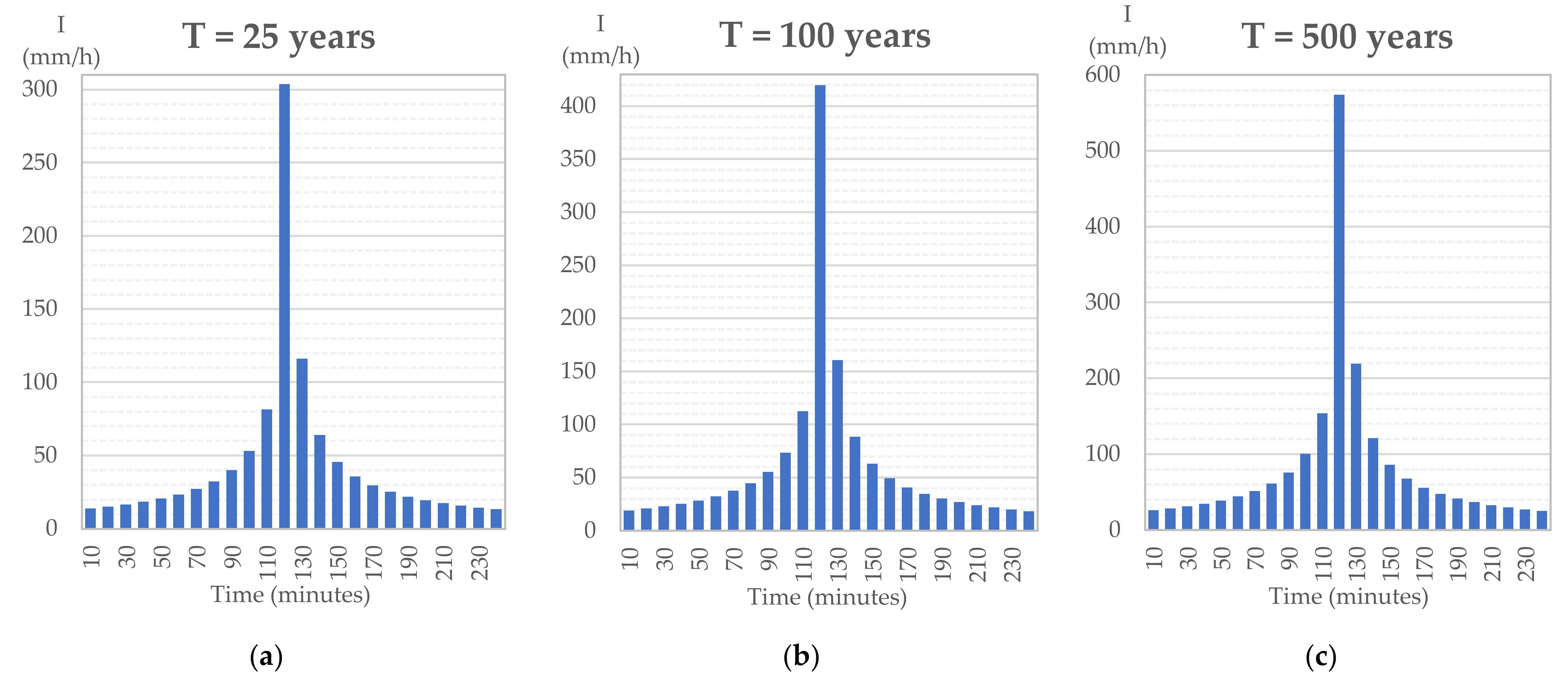
Therefore, the extreme precipitation values do not correspond to the average historical series. For instance, on 3 November 1987, 817 l/m2 were collected in one day in Oliva, that day remaining up to today the highest rainfall record in the Iberian Peninsula. This event occurred with a fairly constant rate of discharge. The maximum intensity in 9 h was 306.4 mm; in 12 h, it was 408.5 mm; and in 18 h, it was 612.8 mm. Although in the area under study, important rainfalls occur regularly, the 1987 storm strongly conditions any statistical adjustment of the historical series. In this work, this statistical adjustment was conducted using the “SQRT-ET max” distribution function [27]:
where k is a shape parameter and α is a scale parameter.
In terms of return periods, these were set following PATRICOVA code [28], a regional Spanish code specially designed as a territorial action plan against flood events in the Valencian Region. This code establishes three possible scenarios corresponding to three return periods: 25 years (high storm probability), 100 years (medium storm probability), and 500 years (low storm probability).
The concentration time (Tc) was computed for each sub-basin according to the maximum path of the water obtained with the DEM prepared. This method ensures each of the subsystems is contributing to the runoff at its drainage point. Temez’s formulation [29] was applied:
where L represents the maximum length of the flow path and J is the average slope at the analyzed section.
2.5. Hydrological Model
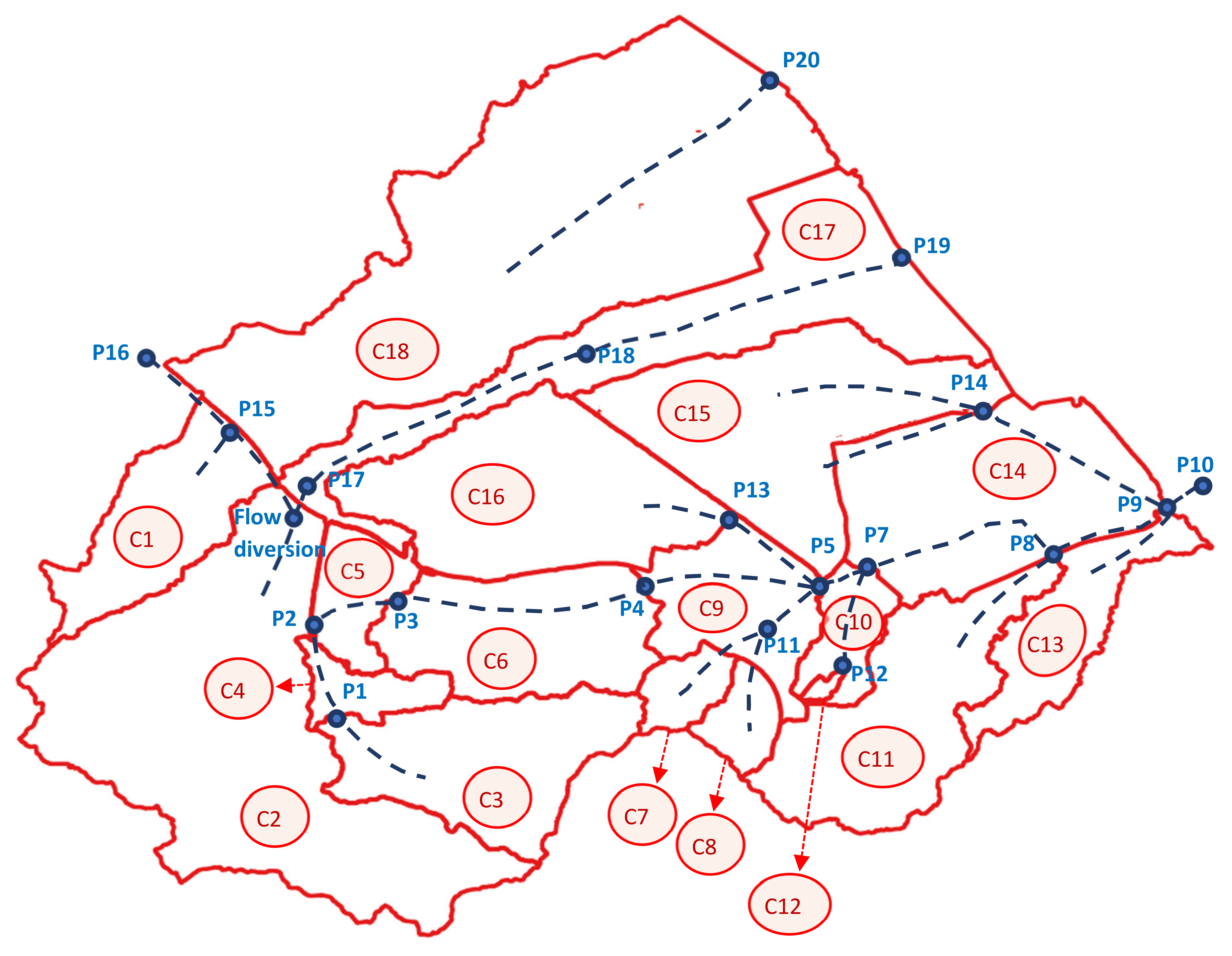
The hydrological model was developed using the HecHMS model [30]. Sub-basin division was transformed into the conceptual operation scheme shown in Figure 6, where connections were established between sub-basins, channels, and fluvial courses. Node P5 represents the entrance to a buried collector that passes under the urban area of Oliva to the west of the town. Node P6 is not represented due to lack of space, but it is located between nodes P5 and P7. At node P2, there is a detour; due to the amplitude of this channel and the barrier effect that this construction generates on its right bank, the analysis considered that all the flow was diverted. Another key point in the model is the one named “Junction”, as it corresponds to the pass of a ravine below the existing highway in the area and where the flow is artificially distributed between the transversal drainage of the highway and a diversion channel that runs towards the Serpis River.
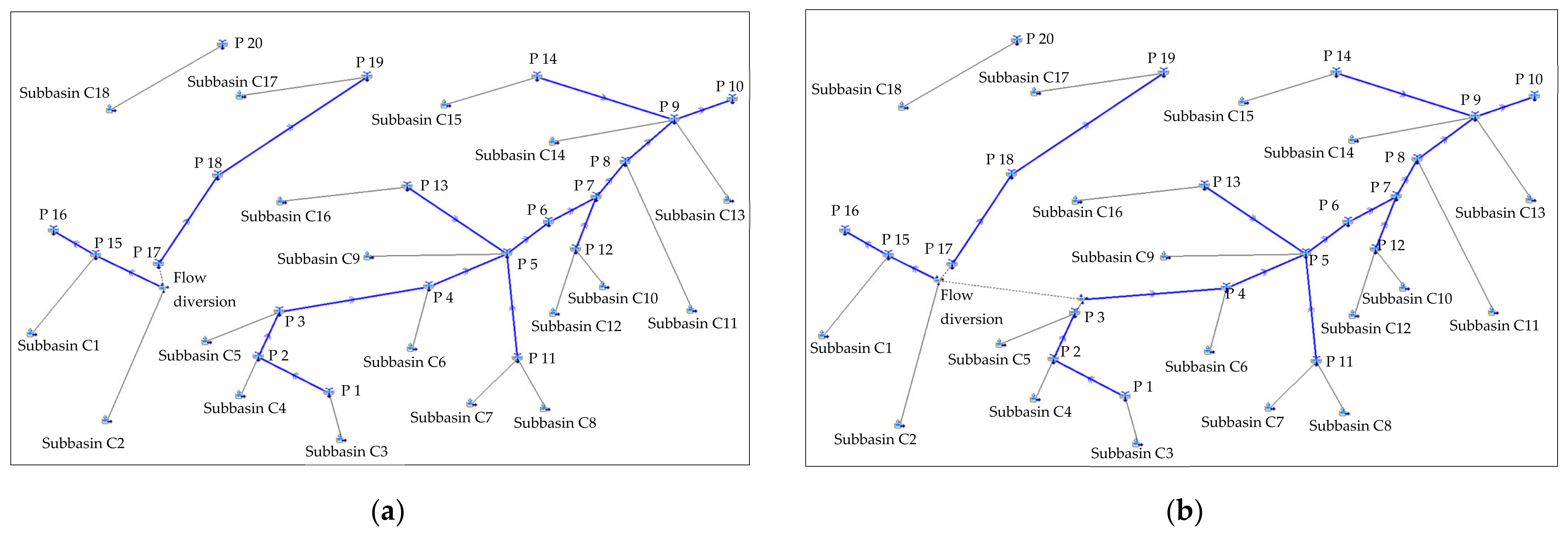
From that conceptual scheme, a hydrological model was developed to reproduce the hydrological behavior of the whole basin. The basin model consisted of a pseudo-distributed model in which each element simulated the hydrological processes as homogeneously as possible [30] and where each sub-basin had its own hydrological parameters. Figure 7a shows the basin model considered for return periods not higher than 100 years, while Figure 7b shows the basin model considered for a return period of 500 years; in this last case, La Font ravine no longer has enough capacity in the surroundings of node P3 and has to discharge its flow excess through the left bank to the west, thus connecting node P3 with nodes P15 and P17. Flows diverted to the west will then flow towards node P17 or will be diverted again to a large channel towards the Serpis River with a maximum capacity of 200 m3/s (nodes P15 and P16).
2.6. Hydraulic Model
The hydraulic simulation was carried out using the HecRas model [31], a worldwide widely contrasted two-dimensional model that allows running calculations in both permanent and transitory regimes. Sufficient extension is needed to realistically reproduce all the hydraulic processes. Besides, identifying valid boundary conditions consistent, reliably to be introduced into the model, is not always easy. A compromise solution must be found between those factors and the goodness/accuracy of the results, as any hydraulic model requires high computing resources even for the actual technical equipment.
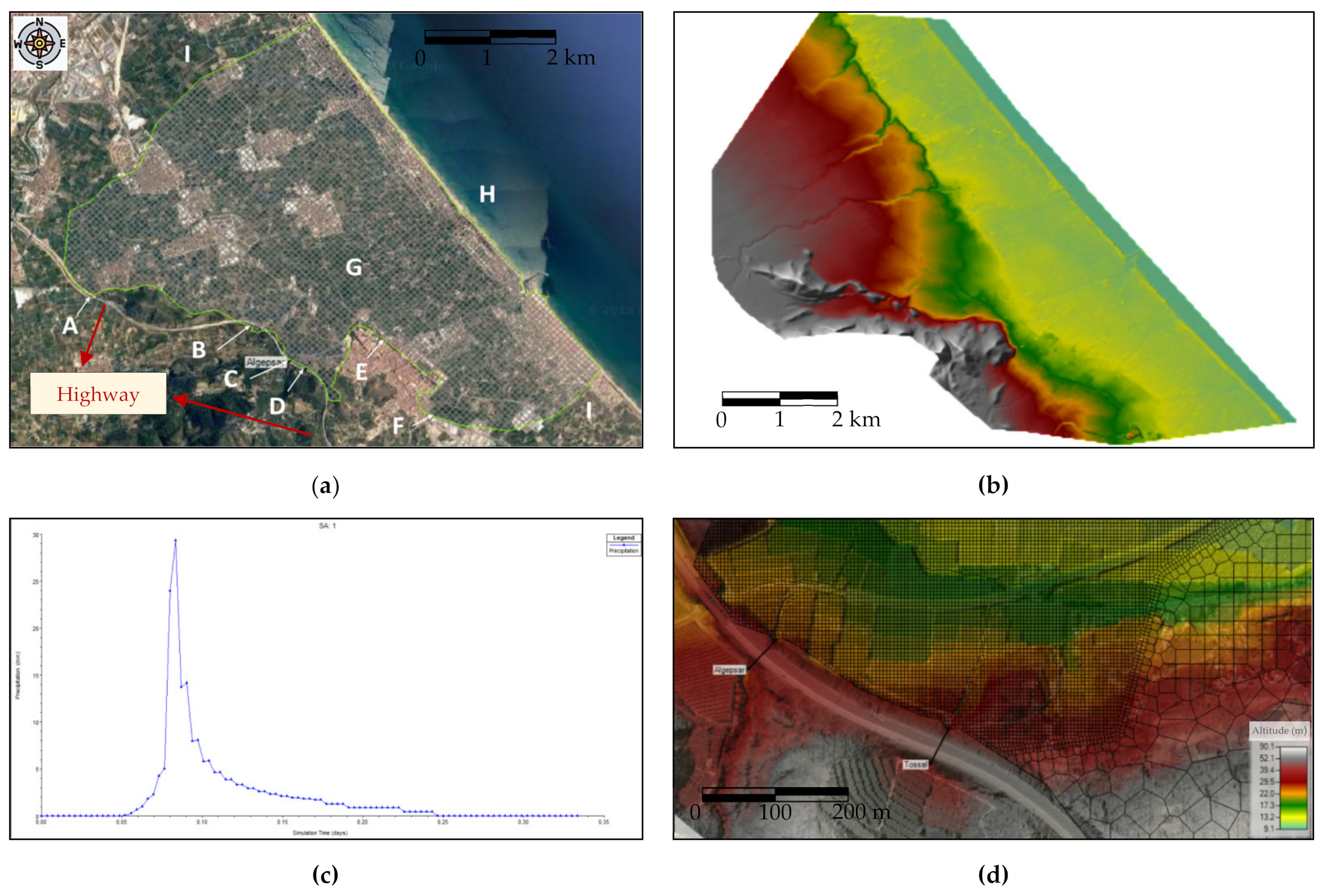
Figure 8a shows the hydraulic model developed for the area under study. Since this is focused on the coastal strip and no flooding problems are found upstream of the existing highway (highlighted in Figure 8a), the analysis could be reduced. Figure 8b shows the DEM shortened and adjusted to the coastal strip used in the hydraulic model. Boundary conditions established are listed in Table 2. All hydrographs were introduced with an interval of input data every 5 minutes. The exit contour conditions considered the coastal dune ridge, which is raised between 1 and 2 meters above the marsh and represents a natural barrier for the water exit.
The urban development of the coastline represents a man-made barrier to be added to the previous one and which prevents the water from being easily evacuated in the event of an extraordinary flood. Internal conditions (condition G in Figure 8a) refer to the precipitations in the sub-basins located in the coastal strip (excluding those corresponding to the Oliva urban area) and were established as the average of the net rainfall obtained in the C9, C11, C13, C14, C15, C16, C17, and C18 sub-basins and calculated for each return period, subtracting from the rain the infiltration capacity of the soil in each interval. As an example, Figure 8c shows the net rainfall for a return period of 25 years.
The roughness values for each area were obtained from classic hydraulic literature [32,33] and field visits, being later adjusted following Spanish codes [34]. Manning number values ranged from 0.019 for smooth concrete channels to 0.100 for urban and industrial areas.
The mesh structure depends on the purpose of the study, the dimensions of the model and the singularities that may appear in it. In this work, a 20 × 20 m mesh was chosen as a general level due to the barely flat surface existing in a large part of the flooding zone and the numerous man-made barriers created by agricultural plots. A more detailed mesh structure was used in areas where the details of the terrain required it: where earthworks existed, the mesh structured lowered to values between 5 × 5 m and 2 × 2 m; in smaller channels or ditches, the resolution was lowered to 1 × 1 m. Figure 8d shows an example of the mesh in the “Junction” point previously mentioned. At that point, downstream does not have a well-defined channel, so a high-resolution mesh was needed to properly reproduce the water surface circulation.
3. Results
3.1. Precipitations
Table 3 lists the maximum precipitation daily values for each return period considered (25, 100, and 500 years). Figure 9 shows the corresponding hyetographs, which were built by the alternate block methodology, with the peak located in the center of the rainfall (approximately at 115 minutes). Note that the hyetographs are given in a discretized way for their use in the hydrological model. Maximum precipitation daily values were corrected by an area factor [26].
Table 4 provides the Curve Number (CN) for each return period and the concentration time (Tc) at each sub-basin as well as for different sub-systems. The concentration time (Tc) of sub-systems was obtained by grouping sub-basins (i.e., maximum path considering a set of sub-basins), so the whole analyzed set was contributing jointly to surface runoff. As can be seen, the most unfavorable concentration time is 3.87 hours, which is found in the C2 + C17 sub-basin system; this is closely followed by the sub-basin system corresponding to La Font ravine (C3 + C4 + C5 + C6 + C9 + C14), whose concentration time is 3.36 h. Both cases indicate that the area presents certain hydrological inertia. Inertia of flows is closely associated with the retention capacity of the basin and the degree of correlation between the different elements of the system [35].
3.2. Hydrological Model
Table 5 lists, for each return period considered and at the different nodes of the hydrological model, the peak flow values, the area drained toward each node, and the total water volume. These results show the generation of violent flood events. The peak flow is obtained at the entrance of Oliva about 2.5 h from the start of the storm. The peak reaches the Mediterranean Sea after 2.67 h. An interesting result is also obtained in the “Junction” point: from a total of 193 m3/s (peak flow), less than 31 m3/s passed through the transversal drainage of the highway (node P17), so nearly 85% (162 m3/s) of it is diverted towards the Serpis River (“Junction” node). Figure 10 shows the hydrographs at those points as well as at node P4, which is also a control point located next to the highway. Note that flow evolutions obtained at nodes P4 and P17 were input boundary conditions of the hydraulic model.
3.3. Hydraulic Model
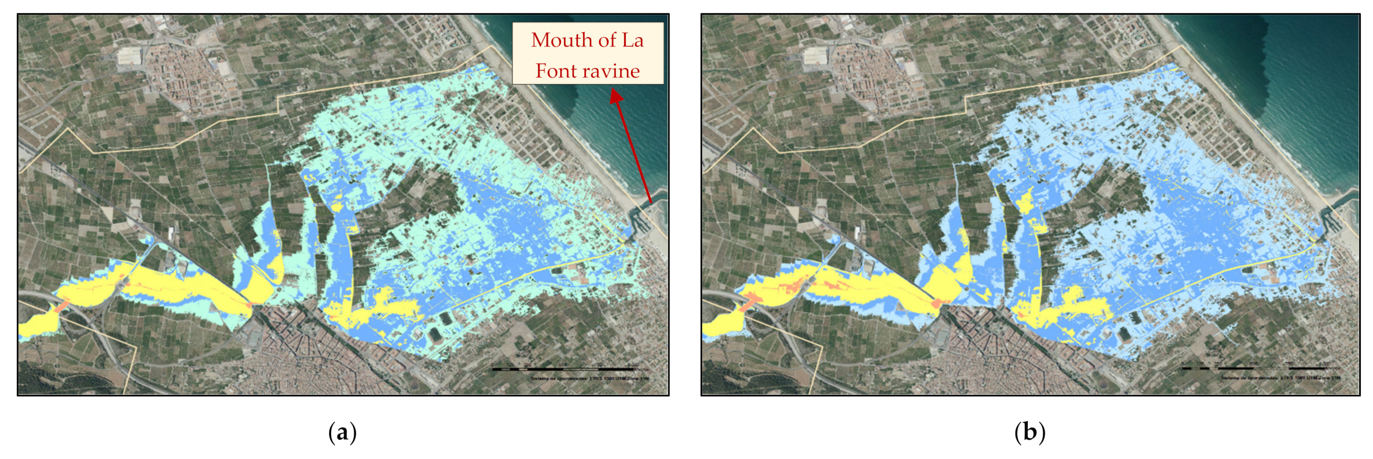
Figure 11 illustrates the extent and importance of the flood for each return period considered. Only depths greater than 0.3 m are represented since values below that level are likely related to the accumulation of rain instead of runoff. As observed, flooding reaches a considerable extension, something expected due to the flat and marshy topography nature of the area under study. Besides, there are zones where depths reach 2 m.
As can be observed, once the water overflows La Font ravine, this cannot return to the riverbed and wide flooding takes place in the area. Besides, roads and paths are transformed into physical barriers to the overflowed water circulation, even though existing culverts on them (included manually on the DEM file) were considered in the model. The dune ridge is the main obstacle that water circulation encounters and it gives rise to a natural barrier that prevents water from draining to the sea. Thus, urban areas found in the coastal strip suffer the flooding consequences.
4. Discussion
4.1. Analysis of the Results
Hydraulic model results show that the water flow has to leave the coast little by little through a unique drainage point located at the harbor of Oliva (highlighted in Figure 11a), which corresponds to the final part of the riverbed of La Font ravine and limits the sub-basin C14 to the south, and sub-basins C11 and C13 to the north (see Figure 4b). The drainage process will therefore need some days to be completed, thus incrementing damage caused by flood events in the area.
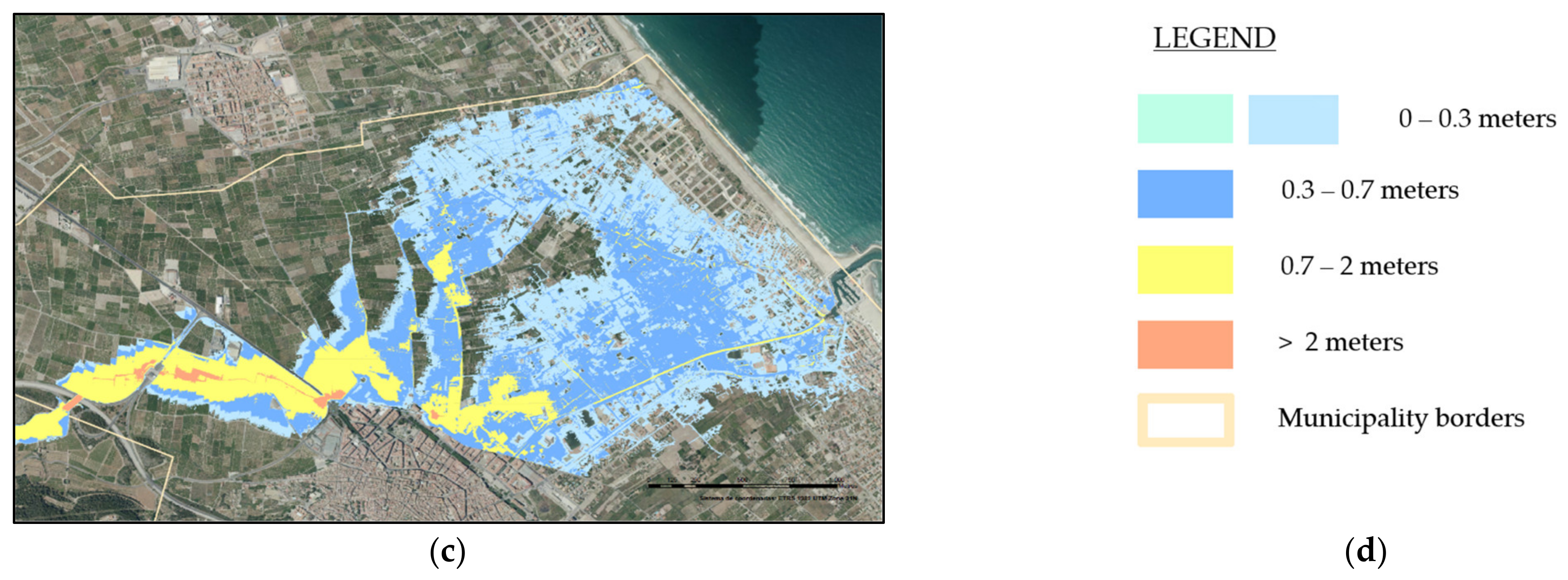
To assess the flooding magnitude, several points were selected as control points to quantify the depth, flow velocity, and its evolution. Figure 12a shows the location of those control points. They correspond to regions of preferential flow circulation, such as areas of overflowing flow (i.e., not strictly the main channels). Figure 12b,c show depth and flow velocity, respectively, at those points.
The analysis of the obtained information allows establishing how the flow system works. Water exceeds the slope of the access branch to the highway (depth control point 1), with a notable accumulation in the adjacent road (depth control point 2). In this area, the flood barely presents a defined channel and circulates overflowing by the existing paths and roads. An important bottleneck effect and the consequent backwater upstream is identified before overcoming a bridge, generating maximum depths of around 2 meters in plots close to the riverbed (depth control point 3). This effect is aggravated by the limited capacity of the urban area to evacuate the flow (given its energy) that already circulates through it from other ravines and from the Oliva urban area itself.
The accumulation of water is also observed in plots located downstream and to the left of the bridge (depth control point 4), generating a small reservoir that is not enough for the level of the subsequent road to be exceeded (depth control point 5). Besides, the flow cannot circulate towards the plots located to the north of it, thus accumulating depth again when it meets enclosure walls and paths (depth control point 6), reaching significant heights. It is from this moment when the flood starts to distribute itself through the marsh towards the lower areas, accumulating water in roads and channels (depth control points 7 and 8), and gradually moving towards the coastal urban area (depth control points 9, 10, 11, and 12). In this populated and flat coastal strip, the flow tends to accumulate due to the impossibility of being drained, given the little or inexistent slope of the land, great energy in the main channels, and a level below the sea at some points.
In terms of water velocities, values greater than 1 m/s are considered to be dangerous due to their erosion and dragging capacity. That value is overcome at velocity control points 2, 3, 5, and 6, although, in some of those points, velocities greater than 1 m/s only occur for return periods of 100 and/or 500 years. Water velocities tend to decrease as the flood advances towards the coast. In the downstream zone, the low velocities are influenced by the boundary condition at the drainage point. The hydraulic regime is subcritical throughout the system, with very low Froude numbers (very far from 1.0). A critical influence of the sea’s boundary condition on the flood (a unique drainage point) is therefore observed. However, these results can be misleading: although at many of the control points the velocities are low, there may be priority flows near certain channels or ditches, which can be dangerous.
It is also interesting to note that the hydraulic simulation shows some atypical results like straight lines vertical to the flow and parallel to roads. This is due to the flat and mash nature of the area and the fact that some of the existing roads are old and have a lack of culverts. Consequently, roads act as water barriers. This causes the roads to retain part of the flood similar to a dam, raising the water level. This ends up spilling overhead at some point. This generates a rather unusual form of flooding. It also makes it unpredictable, since when one of these barriers is broken, the water ends up circulating in places where it was not planned.
4.2. Hydrological Considerations
Commonly, flood studies are developed by adopting a single hydrological model, with hyetographs the solely input modified to obtain the flows associated with each return period [36,37,38,39]. In rare cases, a variation of the runoff coefficient or the Curve Number of the SCS method is also considered in the model for the different return periods. In a mountain region, such an approach is perfectly suitable: once the water arrives at a valley, water is rather improbable to abandon it (water may overflow some terraces, but the water will flow through a similar path). In this case, the amount of water produced by storms has little influence on the circulation water path and consequently, a unique hydrological model can be considered for all return periods.
However, in flat areas, where slopes are very small, the hydrological model depends on the return period and the flows produced. This phenomenon occurred in the case study analyzed, where the natural marsh topography of the area under study gave rise to having two different hydrological models for small and high values of the return period. The issue is of great importance: for small return periods, the amount of water generated by a storm may circulate by channels, which will be completely overflowed in the case of greater return periods. As a result, water paths through the territory may vary as the flows increase and water may circulate by alternative channels, thus varying the connection between nodes. Consequently, in flat coastal areas, the hydrological model cannot be considered unique for the different storms associated with each return period. Hydrological modelling may require several hydrological models associated with different return periods.
In addition, for areas belonging to the Western Mediterranean Sea, the climatological analysis carried out to obtain precipitations and inputs for hydrological models must take into account the special nature of rainfalls in that area (DANA). Traditionally, in flood studies, extreme rains to be used as input are obtained from the historical series recorded at representative stations of the area under study by conducting a statistical adjustment using distribution functions like Gumbel, GEV, and Lognormal-2 [40,41]. In fact, at the end of the last century, the latter two were the more common ones used according to the secretary of the World Meteorological Organization [42].
However, for Western Mediterranean areas, these functions have shown to lead to poor statistical performance and underestimate the forecasts for high return periods, giving rise to an important error [7]. Thus, alternative functions are needed to be used. The one proposed in this work and applied to the case study presented is “SQRT-ET max”. This distribution function was specially proposed [27] for the statistical modelling of maximum daily rains for any return period. It provides more conservative results than the traditional functions and has shown a good ability to reproduce the statistical properties of rains in the Spanish Mediterranean areas, having been verified using Monte Carlo simulation techniques [43,44,45].
4.3. Hydraulic Considerations
The flood analysis of the area under study showed that there is a lack of a main channel or river whose capacity may be exhausted, resulting in overflowing of the water towards the river terraces. On the contrary, the flat and marsh nature of the area makes the water tend to spread over it, covering a great extension. Besides, due to the low slopes, items such as walls, plot divisions, roads, and small embankments, although apparently insignificant, have a great influence on the diversion of floodwaters.
The geometric model used for developing the hydraulic model is a fundamental element for guaranteeing the success of the whole simulation. Thus, a high precision DEM is required, especially in the vertical component, since small geometric variations can cause important distortions in water movement [46]. Commonly, flood studies are conducted by directly implementing the downloaded or obtained DEM without performing any modification [36,47,48]. However, it should be noted that a DEM is obtained by photogrammetric flight and especially by Lidar flights. Usually, this technique does not reflect the correct definition of singular elements, which can condition the flow in flat areas, like culverts, bridges over riverbeds or perimeter plot walls. The correct definition of such elements in the geometric model is essential and this issue is not related to accuracy. For example, for a photogrammetric Lidar flight, a bridge can be interpreted as a transverse dam. A similar situation happens with road transversal drainages. Lidar flights may provide a very precise geometry, but is not consistent enough to be directly entered in a hydraulic model. Dimensions of such elements can be obtained through field measurements and then introduced into the corresponding DEM to obtain consistent results.
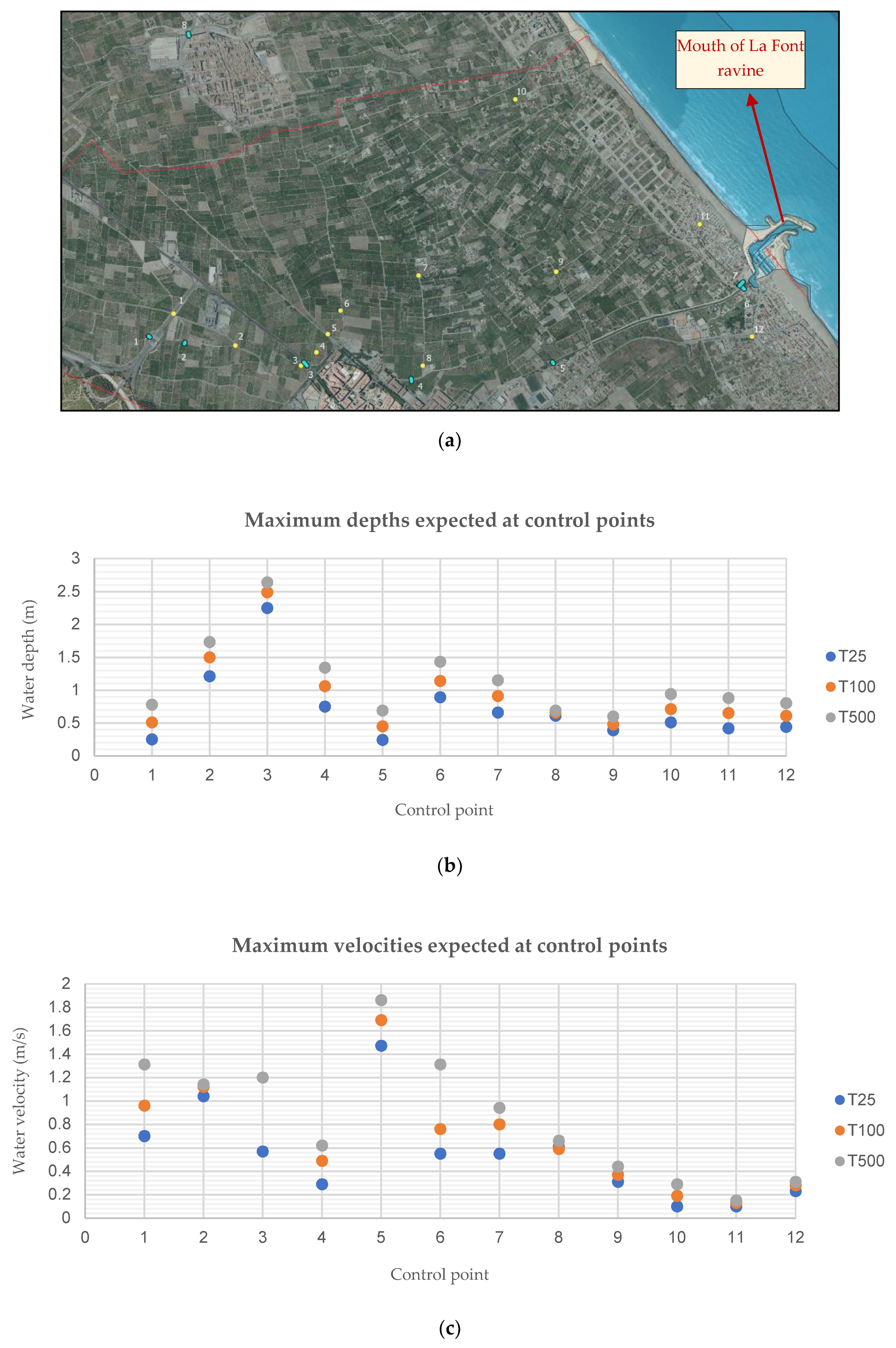
Therefore, flood studies developed in flat and marsh areas require meticulous field work to identify the presence of possible barriers to the flow. These elements must be manually incorporated into the DEM to ensure the reliability of the hydraulic model. In the case study presented in this paper, some corrections were made to the original DEM file to make it as consistent as possible with the hydraulic reality. Corrections were made from field visits. As an example, Figure 13a,b show how the highway transversal drainage was opened manually and the walls of the surrounding plots considered. Those walls were only 40 cm wide and their geometry could not be identified by the Lidar flight, so they had to be manually introduced modifying the DEM file. If these elements had not been introduced, water circulation towards the channel located in the upper part of the image would have been distorted.
Besides, the consideration of these walls is relevant as Figure 13c,d show: in a dry situation, walls do not seem significant, but when a small flood occurs, those walls represent a barrier to the water. If they were neglected, the model would cause the water to circulate between the plots, falling from plot to plot and therefore misrepresenting the real flood. The presence of those elements makes the water circulates along the path as the walls do not allow the water to reach the plots (these lines represent breaklines in the flow). Thus, these small elements that are not properly collected in the original DEM file require an accurate definition before performing the hydraulic simulation. Otherwise, they can distort flooding in flat areas.
In addition, the results of the hydraulic model can vary the approach of the hydrological model, which illustrates the complexity required to study this type of system. In this case study, such issues occur. For example, sub-basins C3 and C4 tend to drain into nodes P2 and P3 for medium and low return periods, while for high return periods, part of the flow of these sub-basins tends to flow northwards, reaching node P17 and P15, which diverts part of the flow towards the Serpis River. This will force the modifying of the hydrological model because of the overflows detected in the hydraulic model. Therefore, hydrological models cannot be considered as an independent and previous step to the hydraulic model. On the contrary, the results of the hydraulic model could force the reconsidering of the flows of the hydrological model. These connections could depend on the return period, which further complicates this analysis.
It is important to note that the features of current software, with good graphic outputs and background aerial images, can generate a false reality of a flood, even though the models contain errors and does not conform to the reality. These errors can be detected with some ease for low or medium return periods, based on experience, but they are very difficult to identify for high return periods due to the lack of evidence on the ground. All in all, a properly flooding simulation in flat and marshy coastal areas needs to ensure consistency in the hydrological and hydraulic models produced. Failure to take care of certain aspects and small details when developing those models may cause relevant errors in the results obtained.
4.4. Climatic Change Considerations
Ephemeral streams are highly dependent on rainfall and terrain characteristics and, therefore, very sensitive to minor changes in these environments [22]. The Eastern Iberian Peninsula is characterized by the abundance of this type of ephemeral streams. Recent studies show that the Mediterranean Sea will be one of the most affected areas by climate change in the coming decades, especially in the west of it [49,50]. Climate change is expected to result in a rise in its water temperature, salinity, and an increase in the sea level. As an indirect consequence, rivers and ravines floods are expected to rise, also increasing the potential risk to infrastructures and urban areas.
There is evidence that climate change is already clearly affecting the temperature and magnitude of extreme rainfall on the European continent and these effects will be greater in the Eastern Iberian Peninsula [51,52], due to its latitude and the physical nature of the convective storms that characterize the region. The “cold drop” phenomenon or DANA generates clouds that reach 10 km in height and produce great rainfalls. A reduction in precipitation is expected due to climate change, which will tend to amplify desertification [53,54], but an intensification of extreme precipitation events is also expected [55]. Both phenomena may be devastating to some areas, causing flooding and erosions of great potential damage.
In recent years, a greater stratification has also been detected in the Mediterranean Sea, both in terms of thermal and saline values [56,57,58]. The Mediterranean Sea waters will be warmer and saltier throughout most of the basin by the end of this century. In the upper sea layer, the mean temperature is estimated to increase by 2.7 °C, while the mean salinity will increase by 0.2 psu [58]. The propagation of these surface anomalies leads to an increase of heat contents of the full water column with a spread between +0.93 to +1.35 °C for the global averaged temperature [59]. In the Western Mediterranean Sea, this stratification seems to be larger than in other regions.
The previous phenomenon will cause not only the global temperature of the Mediterranean Sea to increase, but especially on its surface, which is what provides the humidity required for the formation of the highly vertically developed clouds of convective storms. Thus, the conditions that cause the thermal shock between the warm sea and the continental cold air masses will tend to worsen in the short–medium term. It is therefore expected that in the coming decades, more frequent extreme events of greater magnitude may occur in the east of the Iberian Peninsula [6,60,61].
Climate change will also influence the hydraulic behavior of the floods that occur in the coastal towns. Currently, these areas already present serious drainage difficulties due to their flat and/or marsh nature and the existence of a wide, heavily urbanized dune ridge, which represents a coastal barrier that hinders the water circulation. Thus, the most determining factor will be the rise of the sea level.
The water level at the drainage points significantly affects the hydraulic operation of the system. During a storm and as a consequence of the combined effect of atmospheric pressure and wind [62], the sea level tends to rise. This phenomenon is known as “meteorological tide” and causes the sea level to remain above the overflowed water located in flat areas for a long time. This makes it impossible to drain the flooded areas because the water does not have enough energy to circulate towards the sea. The expected rise in sea level as a result of climate change will worsen this hydraulic operation by negatively modifying the boundary condition at the drainage points [63]. Thus, this rise in the sea level will have a very negative effect, significantly increasing drainage times, which currently tend to be days or even weeks in extreme events.
5. Conclusions
The case study analyzed showed that flood studies in the coastal areas of the Eastern Iberian Peninsula present a relevant singularity. The proximity of the Mediterranean Sea and the orography facilitate sudden great rainfalls with a certain frequency, and the small slope lands (sometimes with the natural characteristics of a marsh) and the great number of infrastructures and constructions existing in many coastal areas of the Iberian Peninsula make the water present a high dispersed movement and difficult drainage. From the analysis conducted in this paper, the following conclusions can be drawn:
- The results of the case study show that at the flat coastal strip, the expected flow for a flood event tends to accumulate due to the little or inexistent slope of the land, the existence of infrastructures and buildings, the great energy in the main channels, and a level below the sea at some points. This makes only one drainage point of the whole system towards the sea exist, located at Oliva harbor. These factors result in flood events causing great damage. Besides, water velocities tend to decrease as the flood advances towards the coast; however, although velocities are low, priority flows near certain channels or ditches may be dangerous.
- Typical convective storms in the Eastern Iberian Peninsula (DANA) result in rainfalls of high intensity of a different nature from the common precipitations, causing typical distribution functions like Gumbel, GEV, and Lognormal-2 not to be suitable for high return periods. Alternative functions like “SQRT-ET max” should be used.
- Due to the flat nature of the areas under study and high rainfall values, the hydrological model may not be unique for each return period analyzed. Different hyetographs, runoff coefficients, and especially flow systems (nodes and connections) must be considered for each return period. Water trajectories through the territory can vary as the flows increase, so the connections between nodes of the hydrological model cannot be considered fixed, but they depend on the different storms associated with each return period.
- The hydraulic model must be as consistent as possible with the real geometry of the area under study. The DEM obtained by photogrammetric flights cannot be directly used for developing the hydraulic model. This must be manually modified to include culverts, opening below the bridges and all transverse drainage as well as every wall or obstacle of small thickness (the usual resolution of DEMs makes it not possible to capture them), which can strongly condition the water movement in flat coastal areas. The dimensions of such elements must be obtained through field measurements. Not doing that may cause the results of the flood studies to be false.
- The results of the hydraulic model for each return period can also vary the approach of the hydrological model and force to modify the hydrological model to take into account the overflows detected. This aspect reinforces the previous conclusion about the hydrological model and also points out the complexity of flood studies in many coastal areas of the Eastern Iberian Peninsula, where the process is iterative.
- Climate change is expected to increase the frequency of extreme events of great rainfalls in the Eastern Iberian Peninsula. Besides, the expected rise in the sea level may result in increasing the drainage difficulty of flat coastal areas, thus also increasing the damage caused by flood events.
Supplementary Materials
The following are available online at www.mdpi.com/2073-4441/13/21/2975/s1, Figure S1: larger version of Figure 2b, Figure S2: larger version of Figure 2d, Figure S3: larger ver-sion of Figure 4b, Figure S4: larger version of Figure 4c, Figure S5: larger version of Figure 4d, Figure S6: larger version of Figure 8a.
Author Contributions
Conceptualization, M.Á.E. and J.G.-R.; Methodology, M.Á.E. and R.P.-G.; Project administration, M.Á.E. and F.J.T.; Software, M.Á.E. and R.P.-G.; Validation, M.Á.E. and R.P.-G.; Formal analysis, M.Á.E. and J.G.-R.; Writing—original draft preparation, M.Á.E. and J.G.-R.; Writing—review and editing, F.J.T. and J.G.-R.; Visualization, F.J.T.; Supervision, F.J.T. All authors have read and agreed to the published version of the manuscript.
Funding
This research received no external funding.
Institutional Review Board Statement
Not applicable.
Informed Consent Statement
Not applicable.
Data Availability Statement
The data presented in this study are available on request from the corresponding author. The data are not publicly available due to privacy reasons.
Acknowledgments
The authors thank Juan Ramón Porta Sancho for his help as a municipal technical coordinator. Juan Ramón Porta Sancho is the head of the Oliva city council technical department of management, urban discipline, and civil protection of the Oliva city council.
Conflicts of Interest
The authors declare no conflict of interest.
References
- Davis, R.E.; Hayden, B.P.; Gay, D.A.; Phillips, W.L.; Jones, G.V. The North Atlantic Subtropical Anticyclone. J. Clim. 1997, 10, 728–744. [Google Scholar] [CrossRef]
- Hénin, R.; Ramos, A.M.; Pinto, J.G.; Liberato, M.L.R. A Ranking of Concurrent Precipitation and Wind Events for the Iberian Peninsula. Int. J. Climatol. 2021, 41, 1421–1437. [Google Scholar] [CrossRef]
- Cardoso, R.M.; Soares, P.M.M.; Miranda, P.M.A.; Belo-Pereira, M. WRF High Resolution Simulation of Iberian Mean and Extreme Precipitation Climate. Int. J. Climatol. 2013, 33, 2591–2608. [Google Scholar] [CrossRef]
- Iberian Climate Atlas; Ministerio de Medio Ambiente, y Medio Rural y Marino; Government of Spain; Catalog of Publications of the General State Administration of Spain: Madrid, Spain, 2011; ISBN 978-84-7837-079-5. [CrossRef]
- Gómez-Navarro, J.J.; Montávez, J.P.; Jiménez-Guerrero, P.; Jerez, S.; Lorente-Plazas, R.; González-Rouco, J.F.; Zorita, E. Internal and External Variability in Regional Simulations of the Iberian Peninsula Climate over the Last Millennium. Clim. Past 2012, 8, 25–36. [Google Scholar] [CrossRef] [Green Version]
- Catálogo. Plan RISP—Agencia Estatal de Meteorología—AEMET. Gobierno de España. Available online: http://www.aemet.es/es/datos_abiertos/catalogo (accessed on 11 August 2021).
- Camarasa Belmonte, A.M.; Soriano Garcí, J.; López-Garcí, M.J. The Effect of Observation Timescales on the Characterisation of Extreme Mediterranean Precipitation. Adv. Geosci. 2010, 26, 61–64. [Google Scholar] [CrossRef] [Green Version]
- Peñarrocha, D.; Estrela, M.J.; Millán, M. Classification of Daily Rainfall Patterns in a Mediterranean Area with Extreme Intensity Levels: The Valencia Region. Int. J. Climatol. 2002, 22, 677–695. [Google Scholar] [CrossRef]
- Ferreira, R.N. Cut-off Lows and Extreme Precipitation in Eastern Spain: Current and Future Climate. Atmosphere 2021, 12, 835. [Google Scholar] [CrossRef]
- Boé, J.; Terray, L.; Cassou, C.; Najac, J. Uncertainties in European Summer Precipitation Changes: Role of Large Scale Circulation. Clim. Dyn. 2009, 33, 265–276. [Google Scholar] [CrossRef]
- Terranova, O.; Gariano, S.L. Analysis of Heavy Rainstorms in the Mediterranean Climate Area. EGU Gen. Assem. Conf. Abstr. 2013, 15, 9798. [Google Scholar]
- Cortesi, N. Variabilità Della Precipitazione Nella Penisola Iberica. Ph.D. Thesis, Universidad de Zaragoza, Zaragoza, Spain, 2013. [Google Scholar]
- Cammeraat, E.L.H. Scale Dependent Thresholds in Hydrological and Erosion Response of a Semi-Arid Catchment in Southeast Spain. Agric. Ecosyst. Environ. 2004, 104, 317–332. [Google Scholar] [CrossRef]
- El Kenawy, A.; López-Moreno, J.I.; Vicente-Serrano, S.M. Trend and Variability of Surface Air Temperature in Northeastern Spain (1920–2006): Linkage to Atmospheric Circulation. Atmos. Res. 2012, 106, 159–180. [Google Scholar] [CrossRef]
- Cohuet, J.B.; Romero, R.; Homar, V.; Ducrocq, V.; Ramis, C. Initiation of a Severe Thunderstorm over the Mediterranean Sea. Atmos. Res. 2011, 100, 603–620. [Google Scholar] [CrossRef]
- Lopez-Bustins, J.A.; Esteban, P.; Labitzke, K.; Langematz, U. The Role of the Stratosphere in Iberian Peninsula Rainfall: A Preliminary Approach in February. J. Atmos. Solar Terrestrial Phys. 2007, 69, 1471–1484. [Google Scholar] [CrossRef] [Green Version]
- Saeed, S.; Van Lipzig, N.; Müller, W.A.; Saeed, F.; Zanchettin, D. Influence of the Circumglobal Wave-Train on European Summer Precipitation. Clim. Dyn. 2014, 43, 503–515. [Google Scholar] [CrossRef]
- Benito, G.; Machado, M. Floods in the Iberian Peninsula. In Changes in Flood Risk in Euope, 1st ed.; Kundzewicz, W., Ed.; CRC Press: Boca Raton, FL, USA, 2012; pp. 372–383. [Google Scholar] [CrossRef]
- Trizio, F.; Torrijo, F.J.; Mileto, C.; Vegas, F. Flood Risk in a Heritage City: Alzira as a Case Study. Water 2021, 13, 1138. [Google Scholar] [CrossRef]
- Lastrada, E.; Cobos, G.; Torrijo, F.J. Analysis of Climate Change’s Eect on Flood Risk. Case Study of Reinosa in the Ebro River Basin. Water 2020, 12, 1114. [Google Scholar] [CrossRef] [Green Version]
- Habitantes Oliva 1900–2020. Available online: https://www.foro-ciudad.com/valencia/oliva/habitantes.html (accessed on 17 August 2021).
- Serrano-Notivoli, R. Rainfall-Runoff Relationships at Event Scale in Western Mediterranean Ephemeral Streams. Hess 2021, 1–22. [Google Scholar] [CrossRef]
- National Geographic Institute. Government of Spain. Plan Nacional de Ortofotografía Aérea. Available online: https://pnoa.ign.es/ (accessed on 18 August 2021).
- U.S. Soil Conservance Service. SCS Curve Number Loss Model. Available online: https://www.hec.usace.army.mil/confluence/hmsdocs/hmstrm/infiltration-and-runoff-volume/scs-curve-number-loss-model (accessed on 18 August 2021).
- National Plan of Observation of the Territory. Government of Spain. Productos SIOSE. Available online: https://www.siose.es/web/guest/productos (accessed on 18 August 2021).
- Drenaje Superficial, Instrucción 5.2-IC; Ministerio de Obras Públicas y Urbanismo, Government of Spain: Madrid, Spain, 1990.
- Etoh, T.; Murota, A.; Nakanishi, M. SQRT-Exponential Type Distribution of Maximum, Hydrologic Frequency Modelling. In Proceedings of the International Symposium on Flood Frequency and Risk Analyses, Lousiana State University, Baton Rouge, LA, USA, 14–17 May 1986; pp. 253–264. [Google Scholar]
- PATRICOVA—Plan de Acción Territorial de Carácter Sectorial Sobre Prevención del Riesgo de Inundación en la Comunitat Valenciana. 2015. Available online: https://politicaterritorial.gva.es/es/web/planificacion-territorial-e-infraestructura-verde/patricova-docs (accessed on 17 August 2021).
- Témez, J.R. Extended and Improved Rational Method. Version of the Highways Administration of Spain. Proc. XXIV Congr. 1991, 33–40. [Google Scholar]
- US Army Corps of Engineers. HEC-HMS. Available online: https://www.hec.usace.army.mil/software/hec-hms/ (accessed on 18 August 2021).
- US Army Corps of Engineers. HEC-RAS. Available online: https://www.hec.usace.army.mil/software/hec-ras/ (accessed on 18 August 2021).
- Chow, V.T. Open-Channel Hydraulics; Davis, H.E., Ed.; Civil Engineering Series; McGraw-Hill: New York, NY, USA, 1959. [Google Scholar]
- Henderson, F.M. Open Channel Flow; Macmillan Publishing Co., INC.: New York, NY, USA, 1966. [Google Scholar]
- Ministerio de Medio Ambiente y Medio Rural y Marino. Government of Spain. Guía Metodológica para el Desarrollo del Sistema Nacional de Cartografía de Zonas Inundables. Available online: https://www.miteco.gob.es/es/agua/publicaciones/guia_metodologica_ZI.aspx (accessed on 18 August 2021).
- Pokojski, W. Inertia of the Catchment Systems Within the Polish Lowlands. Misc. Geogr. 2004, 11, 169–174. [Google Scholar] [CrossRef] [Green Version]
- Mokhtari, E.H.; Remini, B.; Hamoudi, S.A. Modelling of the rain-flow by hydrological modelling software system HEC-HMS-watershed’s case of Wadi Cheliff-Ghrib, Algeria. J. Water L. Dev. 2016, 30, 87–100. [Google Scholar] [CrossRef] [Green Version]
- Bai, Y.; Zhang, Z.; Zhao, W. Assessing the Impact of Climate Change on Flood Events Using HEC-HMS and CMIP5. Water. Air. Soil Pollut. 2019, 230, 6. [Google Scholar] [CrossRef]
- Sarminingsih, A.; Rezagama, A.; Ridwan, M. Simulation of rainfall-runoff process using HEC-HMS model for Garang Watershed, Semarang, Indonesia. J. Phys. Conf. Ser. 2019, 1217, 1. [Google Scholar] [CrossRef]
- Cabrera-Balarezo, J.J.; Timbe-Castro, L.M.; Crespo-Sánchez, P.J. Evaluation of the HEC-HMS model for the hydrological simulation of a paramo basin. DYNA 2019, 86, 338–344. [Google Scholar] [CrossRef] [Green Version]
- Koutsoyiannis, D. On the appropriateness of the gumbel distribution in modelling extreme rainfall. In Hydrological Risk: Recent Advances in Peak River Flow Modelling, Prediction and Real-Time Forecasting. Assessment of the Impacts of Land-Use and Climate Changes, Proceedings of the ESF LESC Exploratory Workshop, Bologna, Italy, 24–25 October 2003; Brath, A., Montanari, A., Toth, E., Eds.; Editoriale Bios: Castrolibero, Italy, 2004; pp. 303–319. [Google Scholar] [CrossRef]
- Galiatsatou, P.; Prinos, P. Outliers and Trend Detection Tests in Rainfall Extremes. Congr. Assoc. Hydraul. Res. 2007, 32, 125. [Google Scholar]
- World Meteorological Organization. Statistical Distributions for Flood Frequency Analysis; WMO Operational Hydrology Report No 33; World Meteorological Organization: Geneva, Switzerland, 1989. [Google Scholar]
- Ferrer, J. Recomendaciones para el Cálculo Hidrometeorológico de Avenidas; CEDEX. Publicaciones del Ministerio de Obras Públicas, Transportes y Medio Ambiente: Madrid, Spain, 1993; p. 77. Available online: https://dialnet.unirioja.es/servlet/libro?codigo=220882 (accessed on 18 August 2021).
- Ferrer, J. El Modelo de Función de Distribución SQRT-ET Max en el Análisis Regional de Máximos Hidrológicos: Aplicación a Lluvias Diarias. Ph.D. Thesis, Universidad Politécnica de Madrid, Madrid, Spain, 1996. [Google Scholar]
- Máximas Lluvias diarias en la España Peninsular. Ministerio de Fomento. 1999. Available online: https://www.mitma.gob.es/recursos_mfom/0610300.pdf (accessed on 10 October 2021).
- Bodoque, J.M.; Guardiola-Albert, C.; Aroca-Jiménez, E.; Eguibar, M.Á.; Martínez-Chenoll, M.L. Flood Damage Analysis: First Floor Elevation Uncertainty Resulting from LiDAR-Derived Digital Surface Models. Remote Sens. 2016, 8, 604. [Google Scholar] [CrossRef] [Green Version]
- Prütz, R.; Månsson, P. A GIS-based approach to compare economic damages of fluvial flooding in the Neckar River basin under current conditions and future scenarios. Nat. Hazards 2021, 108, 1807–1834. [Google Scholar] [CrossRef]
- Aksoy, H.; Ozgur Kirca, V.S.; Burgan, H.I.; Kellecioglu, D. Hydrological and hydraulic models for determination of flood-prone and flood inundation areas. IAHS-AISH Proc. Rep. 2016, 373, 137–141. [Google Scholar] [CrossRef] [Green Version]
- Vargas-Yáñez, M.; Moya, F.; García-Martínez, M.C.; Tel, E.; Zunino, P.; Plaza, F.; Salat, J.; Pascual, J.; López-Jurado, J.L.; Serra, M. Climate Change in the Western Mediterranean Sea 1900–2008. J. Mar. Syst. 2010, 82, 171–176. [Google Scholar] [CrossRef]
- Lastrada, E.; Garzón-Roca, J.; Cobos, G.; Torrijo, F.J. A Decrease in the Regulatory Effect of Snow-Related Phenomena in Spanish Mountain Areas Due to Climate Change. Water 2021, 13, 1550. [Google Scholar] [CrossRef]
- Viceto, C.; Pereira, S.C.; Rocha, A. Climate Change Projections of Extreme Temperatures for the Iberian Peninsula. Atmosphere 2019, 10, 229. [Google Scholar] [CrossRef] [Green Version]
- García-Martín, A.; Paniagua, L.L.; Moral, F.J.; Rebollo, F.J.; Rozas, M.A. Spatiotemporal Analysis of the Frost Regime in the Iberian Peninsula in the Context of Climate Change (1975–2018). Sustainability 2021, 13, 8491. [Google Scholar] [CrossRef]
- Andrade, C.; Contente, J.; Santos, J.A. Climate Change Projections of Aridity Conditions in the Iberian Peninsula. Water 2021, 13, 2035. [Google Scholar] [CrossRef]
- Rasilla, D.F.; Garmendia, C.; García-Codron, J.C. Climate Change Projections of Streamflow in the Iberian Peninsula. Int. J. Water Resour. Dev. 2013, 29, 184–200. [Google Scholar] [CrossRef]
- Cardoso Pereira, S.; Marta-Almeida, M.; Carvalho, A.C.; Rocha, A. Extreme Precipitation Events under Climate Change in the Iberian Peninsula. Int. J. Climatol. 2020, 40, 1255–1278. [Google Scholar] [CrossRef]
- Iona, A.; Theodorou, A.; Sofianos, S.; Watelet, S.; Troupin, C.; Beckers, J.-M. Mediterranean Sea Climatic Indices: Monitoring Long Term Variability and Climate Changes. Earth Syst. Sci. Data Discuss. 2018, 10, 1–18. [Google Scholar] [CrossRef] [Green Version]
- Sannino, G.; Carillo, A.; Iacono, R.; Napolitano, E.; Palma, M.; Pisacane, G. Modelling Present and Future Climate in the Mediterranean Sea: A Focus on Sea-Level Change. Clim. Dyn. 2021. in review. [Google Scholar] [CrossRef]
- Parras-Berrocal, I.M.; Vazquez, R.; Cabos, W.; Sein, D.; Manañes, R.; Perez-Sanz, J.; Izquierdo, A. The Climate Change Signal in the Mediterranean Sea in a Regionally Coupled Atmosphere-Ocean Model. Ocean Sci. 2020, 16, 743–765. [Google Scholar] [CrossRef]
- Adloff, F.; Somot, S.; Sevault, F.; Jordà, G.; Aznar, R.; Déqué, M.; Herrmann, M.; Marcos, M.; Dubois, C.; Padorno, E.; et al. Mediterranean Sea Response to Climate Change in an Ensemble of Twenty First Century Scenarios. Clim. Dyn. 2015, 45, 2775–2802. [Google Scholar] [CrossRef]
- Camarasa-Belmonte, A.M.; Rubio, M.; Salas, J. Rainfall Events and Climate Change in Mediterranean Environments: An Alarming Shift from Resource to Risk in Eastern Spain. Nat. Hazards 2020, 103, 423–445. [Google Scholar] [CrossRef]
- Viceto, C.; Marta-Almeida, M.; Rocha, A. Future Climate Change of Stability Indices for the Iberian Peninsula. Int. J. Climatol. 2017, 37, 4390–4408. [Google Scholar] [CrossRef]
- Krestenitis, Y.; Pytharoulis, I.; Karacostas, T.S.; Androulidakis, Y.; Makris, C.; Kombiadou, K.; Tegoulias, I.; Baltikas, V.; Kotsopoulos, S.; Kartsios, S. Severe Weather Events and Sea Level Variability Over the Mediterranean Sea: The WaveForUs Operational Platform. In Perspectives on Atmospheric Sciences; Karacostas, T.S., Alkiviadis, F.B., Panagiotis, T.N., Eds.; Springer International Publishing: Cham, Switzerland, 2017; pp. 63–68. [Google Scholar] [CrossRef]
- Soto-Navarro, J.; Jordá, G.; Amores, A.; Cabos, W.; Somot, S.; Sevault, F.; Macías, D.; Djurdjevic, V.; Sannino, G.; Li, L.; et al. Evolution of Mediterranean Sea Water Properties under Climate Change Scenarios in the Med-CORDEX Ensemble. Clim. Dyn. 2020, 54, 2135–2165. [Google Scholar] [CrossRef] [Green Version]
Figure 1.
Examples of flooding effects in the area under study (Oliva, Spain): (a) flooding in 1972; (b) flooding in 1987; (c) flooding in 1997; (d) flooding in 2013.
Figure 1.
Examples of flooding effects in the area under study (Oliva, Spain): (a) flooding in 1972; (b) flooding in 1987; (c) flooding in 1997; (d) flooding in 2013.

Figure 2.
Geographical Setting and Geological Framework: (a) location of the town of Oliva; (b) geological framework in the area; (c) aerial view of the area under study (image from Landsat-Copernicus, data SIO, NOAA, US Navy, NGA, GEBCO, 2021, Google Earth); (d) urbanization of the area. All maps are oriented to the North. An extended larger version of Figure 2b,d can be found in the Supplementary Material.

Figure 3.
Methodological scheme for developing flood studies at flat coastal areas of the Eastern Iberian Peninsula.
Figure 3.
Methodological scheme for developing flood studies at flat coastal areas of the Eastern Iberian Peninsula.

Figure 4.
Territory analysis of the area under study: (a) DEM; (b) division of the area into sub-basins; (c) sub-basins defined overlapped with the geological epoch-period and orography; (d) land uses of SIOSE map [25]. All maps are oriented to the North. An extended larger version of Figure 4b–d, can be found in the Supplementary Material.

Figure 5.
Average precipitations per year in the area under study.

Figure 6.
Conceptual operation scheme.

Figure 7.
Hydrological model using HecHMS: (a) Model for return periods not higher than 100 years; (b) Model for a return period of 500 years.
Figure 7.
Hydrological model using HecHMS: (a) Model for return periods not higher than 100 years; (b) Model for a return period of 500 years.

Figure 8.
Hydraulic model developed: (a) HecRas 2D model with boundary condition (see Table 2); (b) DEM shortened and adjusted to the coastal strip used in the simulations; (c) net rainfall for a return period of 25 years; (d) mesh structure around the “Junction” point. All maps are oriented to the North. An extended larger version of Figure 8a can be found int the Supplementary Material.

Figure 9.
Hyetographs for each return period analyzed: (a) 25 years; (b) 100 years; (c) 500 years.

Figure 10.
Hydrographs at nodes located next to the highway: (a) P4 node; (b) P17 node; (c) Junction node upstream P17. Vertical axis: flow. Horizontal axis: time. Continuous, dashed and dotted lines corresponds to the return periods T = 25 years, T = 100 years and T = 500 years, respectively.
Figure 10.
Hydrographs at nodes located next to the highway: (a) P4 node; (b) P17 node; (c) Junction node upstream P17. Vertical axis: flow. Horizontal axis: time. Continuous, dashed and dotted lines corresponds to the return periods T = 25 years, T = 100 years and T = 500 years, respectively.

Figure 11.
Hydraulic model results. Maximum depths reached for different return periods: (a) 25 years; (b) 100 years; (c) 500 years; (d) relationship between colors and depths values. All maps are oriented to the North.
Figure 11.
Hydraulic model results. Maximum depths reached for different return periods: (a) 25 years; (b) 100 years; (c) 500 years; (d) relationship between colors and depths values. All maps are oriented to the North.


Figure 12.
Flooding magnitude assessment for the different return periods considered (25, 100, and 500 years): (a) location of the control point selected in yellow color; (b) depth expected at each control point; (c) water velocity expected at each control point.
Figure 12.
Flooding magnitude assessment for the different return periods considered (25, 100, and 500 years): (a) location of the control point selected in yellow color; (b) depth expected at each control point; (c) water velocity expected at each control point.

Figure 13.
Example of modifications conducted in the hydraulic model for ensuring consistency: (a) detail of the opening of the transverse drainage below the highway and inclusion of agricultural plot walls in the surrounding area (breaklines in grey color); (b) mesh structure including the presence of the aforementioned elements; (c) image of the area in flooding situations; (d) image of the area in a dry situation.


Table 1.
Sub-basin areas and their centroid elevation. Description gives the local name of the riverbed; note that the same riverbed is sometimes named with different local names through its run (e.g., C3, C6, C9, and C14 correspond to the same riverbed).
Table 1.
Sub-basin areas and their centroid elevation. Description gives the local name of the riverbed; note that the same riverbed is sometimes named with different local names through its run (e.g., C3, C6, C9, and C14 correspond to the same riverbed).
| Sub-Basin | Description | Area (m2) | Elevation (m) |
|---|---|---|---|
| C1 | Barranquet ravine upstream | 1,493,058 | 44.8 |
| C2 | Palmera ravine upstream | 5,959,155 | 58.3 |
| C3 | Muntanyelles ravine | 2,068,349 | 162.7 |
| C4 | Village of La Font d´en Carròs (upstream) | 428,260 | 60.6 |
| C5 | Village of La Font d´en Carròs (downstream) | 655,084 | 39.7 |
| C6 | Ravine of La Font | 1,985,259 | 34.0 |
| C7 | Ravine of L´Algepsar | 369,009 | 143.4 |
| C8 | Tossal Gros ravine | 388,793 | 102.3 |
| C9 | Ravine of La Mitjana | 1,330,276 | 10.8 |
| C10 | North Oliva town | 548,550 | 16.1 |
| C11 | South Oliva town and Alfadalí ravine | 2,343,662 | 13.6 |
| C12 | Ravine of Tossal de la Creu Alto. | 43,730 | 71.4 |
| C13 | Mare ditch | 1,163,342 | 2.8 |
| C14 | Burguera valley | 2,962,216 | 1.9 |
| C15 | Terra Nova valley + Piles ravine downstream | 3,073,918 | 2.7 |
| C16 | Piles ravine upstream | 2,961,022 | 20.3 |
| C17 | Palmera ravine downstream | 3,367,857 | 16.2 |
| C18 | Barranquet ravine downstream | 7,737,696 | 17.5 |
Table 2.
Boundary conditions established in the hydraulic model (see Figure 8a).
Table 2.
Boundary conditions established in the hydraulic model (see Figure 8a).
| Id. | Condition | Description | Slope (m/m) |
|---|---|---|---|
| A | Inlet | Hydrograph at P17 | 0.0001 |
| B | Inlet | Hydrograph at P4 | 0.002 |
| C | Inlet | Hydrograph at the exit of C7 | 0.015 |
| D | Inlet | Hydrograph at the exit of C8 | 0.124 |
| E | Inlet | Hydrograph at P12 | 0.005 |
| F | Inlet | Hydrograph at the exit of C11 | 0.001 |
| H | Outlet | Meteorological tide | --- |
| I | Outlet | Connection with the marsh | 0.0001 |
Table 3.
Maximum daily precipitation obtained for each return period.
| Return Period | Daily Precipitation |
|---|---|
| 25 years | 260.54 mm |
| 100 years | 360.12 mm |
| 500 years | 491.79 mm |
Table 4.
Curve Number (CN) and concentration time (Tc) at each sub-basin and for different sub-systems.
Table 4.
Curve Number (CN) and concentration time (Tc) at each sub-basin and for different sub-systems.
| Sub-Basin | CN, T = 25 Years | CN, T = 100 Years | CN, T = 500 Years | Tc (min) |
|---|---|---|---|---|
| C1 | 70.92 | 66.15 | 61.46 | 87.1 |
| C2 | 60.57 | 55.18 | 50.12 | 124.7 |
| C3 | 59.04 | 53.59 | 48.52 | 55.2 |
| C4 | 64.73 | 59.53 | 54.56 | 39.6 |
| C5 | 64.66 | 59.45 | 54.47 | 37.5 |
| C6 | 59.10 | 53.66 | 48.59 | 77.5 |
| C7 | 54.69 | 49.17 | 44.12 | 21.9 |
| C8 | 58.06 | 52.59 | 47.52 | 37.9 |
| C9 | 63.35 | 58.07 | 53.06 | 61.7 |
| C10 | 83.33 | 80.02 | 76.58 | 50.6 |
| C11 | 73.93 | 69.44 | 64.97 | 79.3 |
| C12 | 52.81 | 47.28 | 42.26 | 11.8 |
| C13 | 78.37 | 74.38 | 70.32 | 148.3 |
| C14 | 68.83 | 63.90 | 59.09 | 145.0 |
| C15 | 69.11 | 64.19 | 59.40 | 132.1 |
| C16 | 66.32 | 61.20 | 56.29 | 82.0 |
| C17 | 69.43 | 64.54 | 59.77 | 152.7 |
| C18 | 69.66 | 64.79 | 60.03 | 184.0 |
| C2 + C17 | - | - | - | 232.4 |
| C3 + C4 + C5 + C6 + C9 + C14 | - | - | - | 201.8 |
| C16 + C9 + C14 | - | - | - | 172.7 |
| C12 + C10 + C14 | - | - | - | 134.5 |
| C11 + C14 | - | - | - | 151.6 |
| C13 + C14 | - | - | - | 149.7 |
Table 5.
Hydrological model results.
| Node | Area Drained (km2) | T = 25 Years | T = 100 Years | T = 500 Years | |||
|---|---|---|---|---|---|---|---|
| Peak Flow (m3/s) | Water Volume (1000 m3) | Peak Flow (m3/s) | Water Volume (1000 m3) | Peak Flow (m3/s) | Water Volume (1000 m3) | ||
| P1 | 2.07 | 28.02 | 103.6 | 54.26 | 214.3 | 95.34 | 347.5 |
| P2 | 2.5 | 34.01 | 128.2 | 65.04 | 264.1 | 113.35 | 427.4 |
| P3 | 3.15 | 41.62 | 165.7 | 78.12 | 340.2 | 135.69 | 549.4 |
| P4 | 5.14 | 61.27 | 266.0 | 114.22 | 547.2 | 200.29 | 883.4 |
| P5 | 10.19 | 120.85 | 552.0 | 222.76 | 1127.7 | 388.42 | 1814.6 |
| P6 | 10.19 | 120.68 | 552.0 | 223.14 | 1127.7 | 387.79 | 1814.6 |
| P7 | 10.78 | 133.26 | 625.6 | 242.62 | 1246.0 | 415.71 | 1978.4 |
| P8 | 13.12 | 164.58 | 791.0 | 296.56 | 1570.2 | 506.61 | 2488.3 |
| P9 | 20.32 | 250.26 | 1263.1 | 450.86 | 2506.2 | 768.04 | 3970.5 |
| P10 | 20.32 | 248.84 | 1263.1 | 451.03 | 2506.2 | 768.36 | 3970.5 |
| P13 | 2.96 | 41.72 | 176.2 | 77.11 | 355.4 | 133.28 | 568.0 |
| P11 | 0.76 | 11.31 | 35.6 | 22.87 | 74.3 | 41.10 | 121.1 |
| P12 | 0.59 | 23.99 | 73.6 | 34.35 | 118.2 | 48.33 | 163.7 |
| P14 | 3.07 | 37.05 | 194.9 | 67.09 | 389.1 | 114.68 | 618.3 |
| P15 | 7.45 | 66.92 | 338.4 | 122.85 | 693.9 | 223.64 | 1137.2 |
| P16 | 7.45 | 66.86 | 338.4 | 123.15 | 693.9 | 223.59 | 1137.2 |
| P17 | 5.96 | 12.17 | 70.0 | 23.12 | 139.3 | 30.65 | 203.1 |
| P18 | 5.96 | 12.17 | 70.0 | 23.07 | 139.3 | 30.65 | 203.1 |
| P19 | 3.37 | 50.12 | 285.1 | 91.17 | 568.2 | 146.35 | 884.2 |
| P20 | 7.74 | 78.82 | 496.8 | 140.52 | 988.9 | 238.38 | 1570.1 |
| Junction | 5.96 | 47.3 | 239.8 | 86.89 | 498.4 | 162.08 | 827.8 |
Publisher’s Note: MDPI stays neutral with regard to jurisdictional claims in published maps and institutional affiliations. |
© 2021 by the authors. Licensee MDPI, Basel, Switzerland. This article is an open access article distributed under the terms and conditions of the Creative Commons Attribution (CC BY) license (https://creativecommons.org/licenses/by/4.0/).
Share and Cite
MDPI and ACS Style
Eguibar, M.Á.; Porta-García, R.; Torrijo, F.J.; Garzón-Roca, J. Flood Hazards in Flat Coastal Areas of the Eastern Iberian Peninsula: A Case Study in Oliva (Valencia, Spain). Water 2021, 13, 2975. https://doi.org/10.3390/w13212975
AMA Style
Eguibar MÁ, Porta-García R, Torrijo FJ, Garzón-Roca J. Flood Hazards in Flat Coastal Areas of the Eastern Iberian Peninsula: A Case Study in Oliva (Valencia, Spain). Water. 2021; 13(21):2975. https://doi.org/10.3390/w13212975
Chicago/Turabian StyleEguibar, Miguel Ángel, Raimon Porta-García, Francisco Javier Torrijo, and Julio Garzón-Roca. 2021. "Flood Hazards in Flat Coastal Areas of the Eastern Iberian Peninsula: A Case Study in Oliva (Valencia, Spain)" Water 13, no. 21: 2975. https://doi.org/10.3390/w13212975
Note that from the first issue of 2016, this journal uses article numbers instead of page numbers. See further details here.