
Potential Impact of Climate Change Analysis on the Management of Water Resources under Stressed Quantity and Quality Scenarios

 ,
,  ,
,
Abstract
:1. Introduction
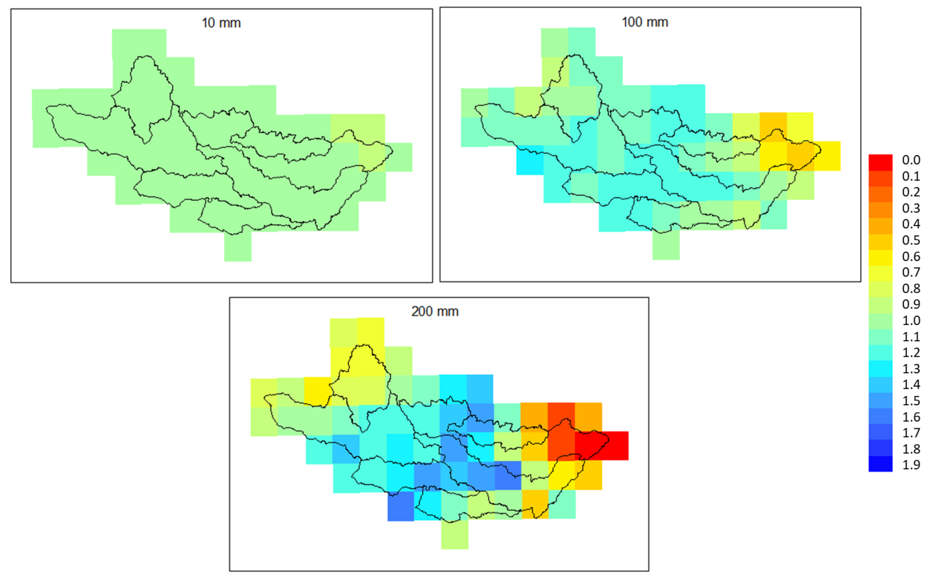
2. Materials and Methods
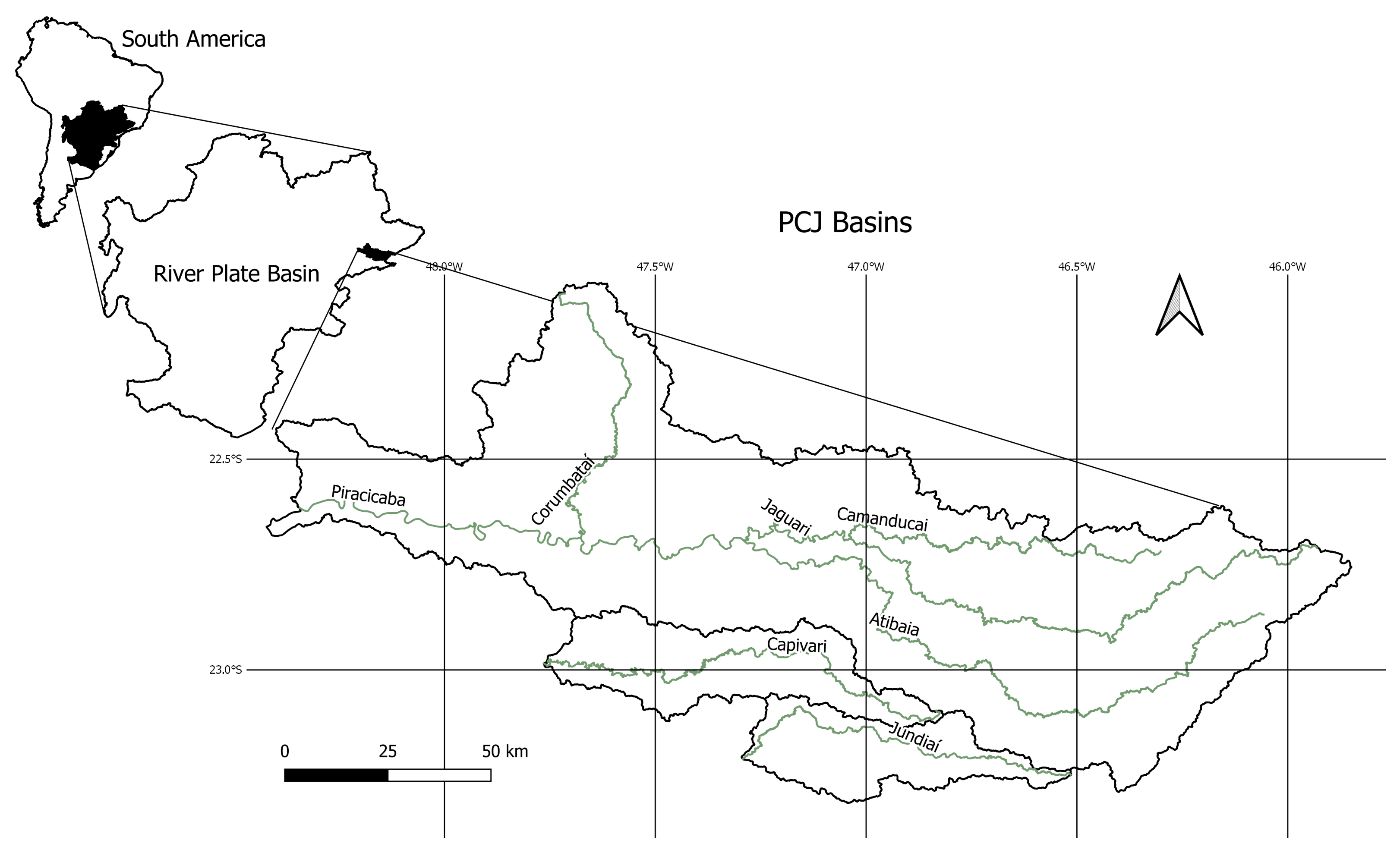
2.1. Study Area
2.2. Runoff
2.3. Water Uses
- 2020: This scenario considers a population of 5,792,141 citizens, estimated by geometric growth rates; base year 2020 scenarios were calibrated with 130 existing water treatment plants in the watershed and 158 wastewater treatment plants. The water demand is nearly 30.51 m³/s, and effluent disposal is around 12.58 m³/s, with current organic matter collection, treatment, and removal rates observed throughout the plants.
- 2035: The main difference in the 2035 scenario is a biochemical oxygen demand (BOD) removal efficiency threshold of 80% [20]; aside from this, from a total population of 7,065,471 citizens, and 130 and 169 water and wastewater treatment plants, respectively, we verified a water demand of 31.72 m³/s and a wastewater discharge of 13.49 m³/s, with a progression of requirements, treatment, and discharge compatible with future predictions estimated to the targeted management horizon.
2.4. PCJ DSS
- Lateral contribution
- Accumulation
- Advection
- Dispersion
- First-order decay
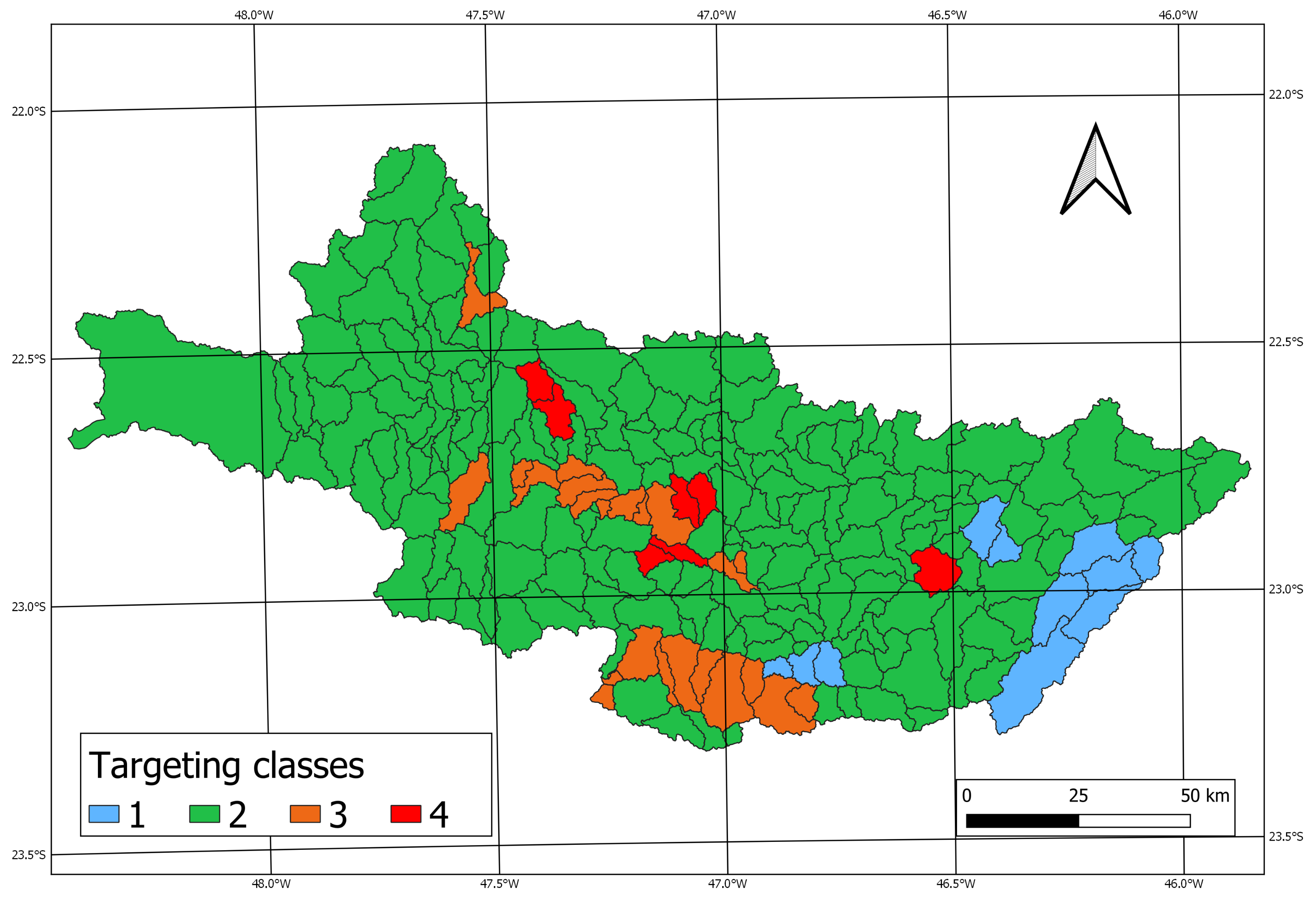
2.5. Framework-Based Indicators
- Class 1: rivers intended for water supply after simple treatment;
- Class 2: rivers intended for water supply after conventional treatment;
- Class 3: rivers intended for water supply after advanced treatment;
- Class 4: rivers intended for navigation and landscape harmony only.
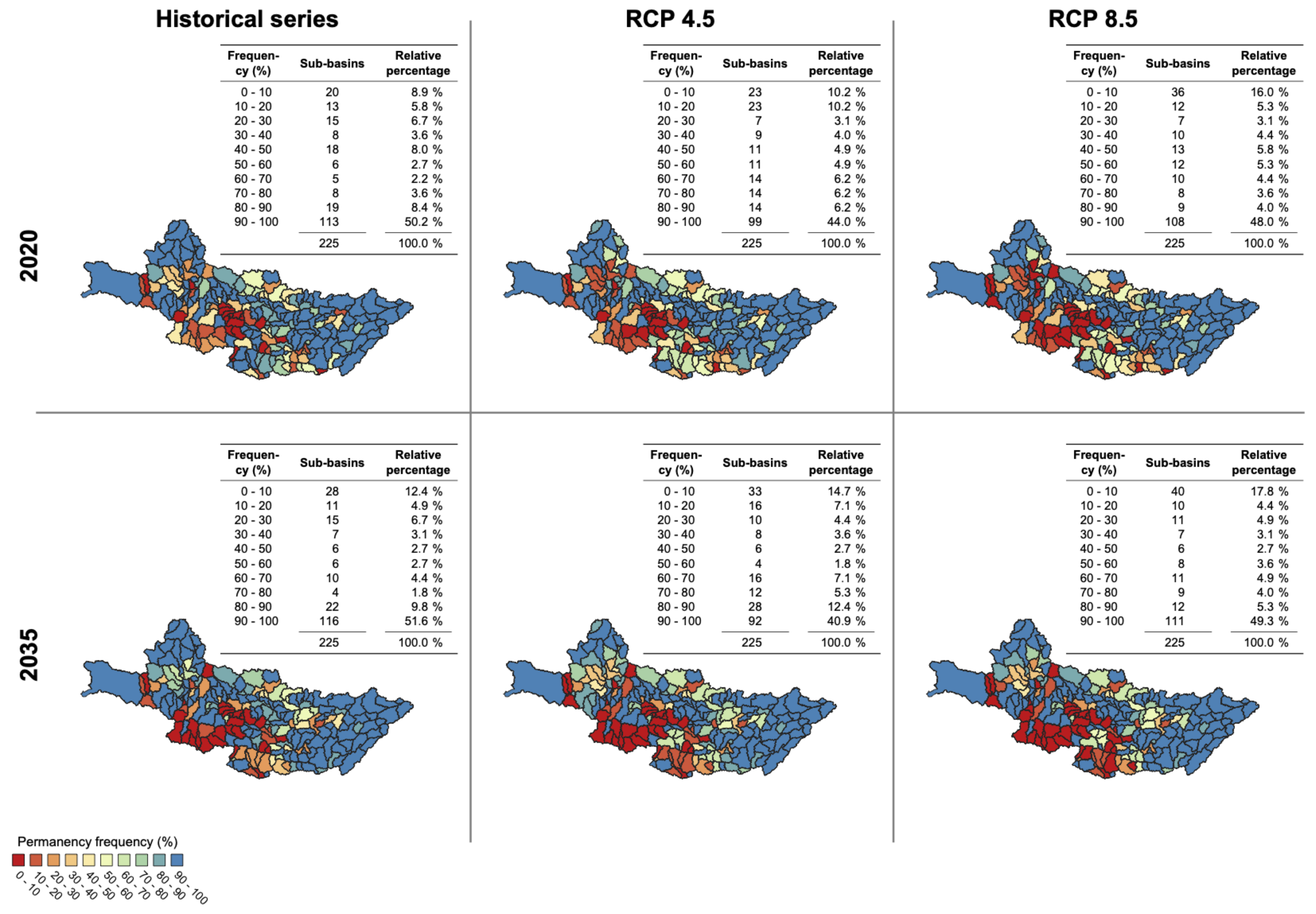
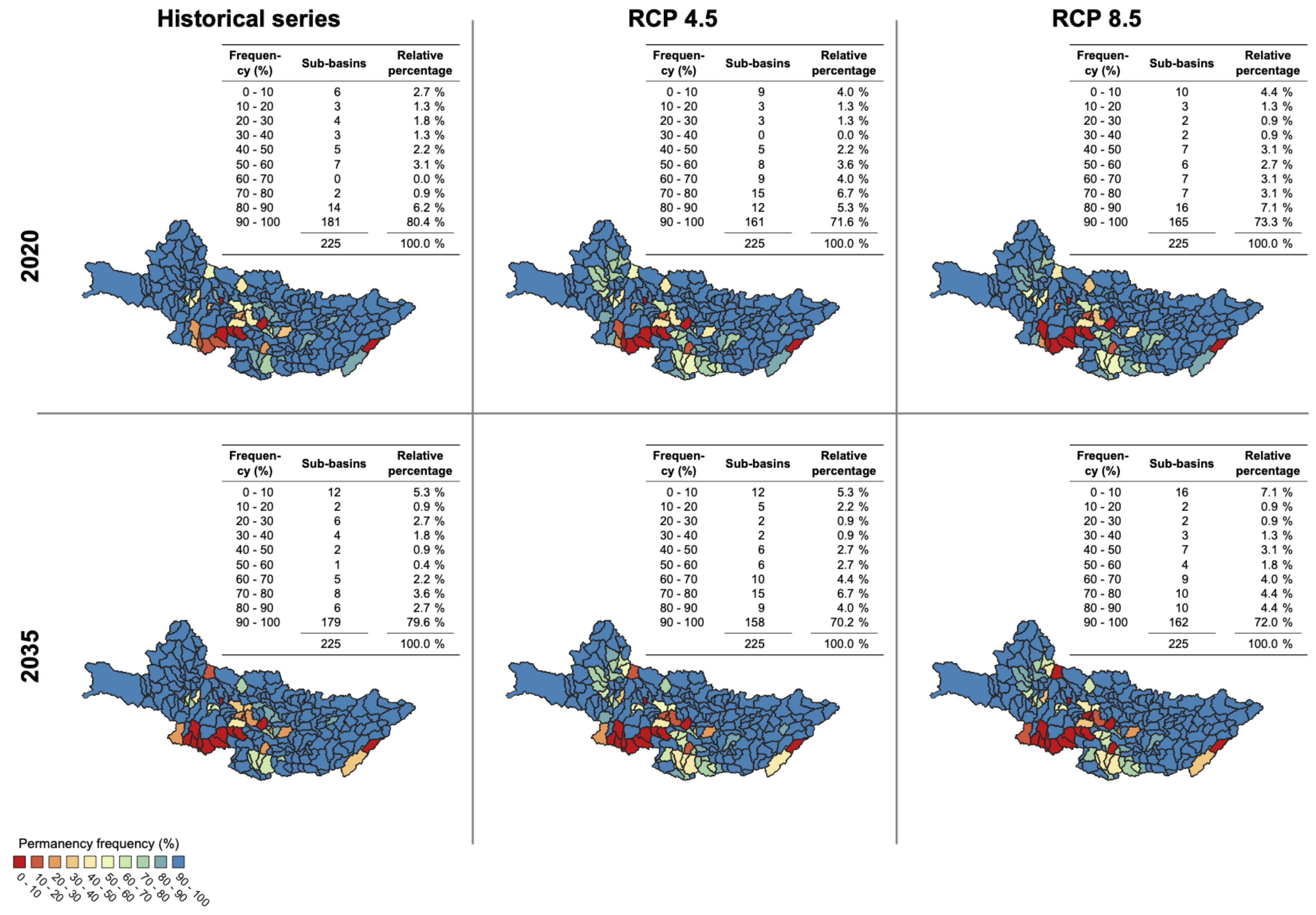
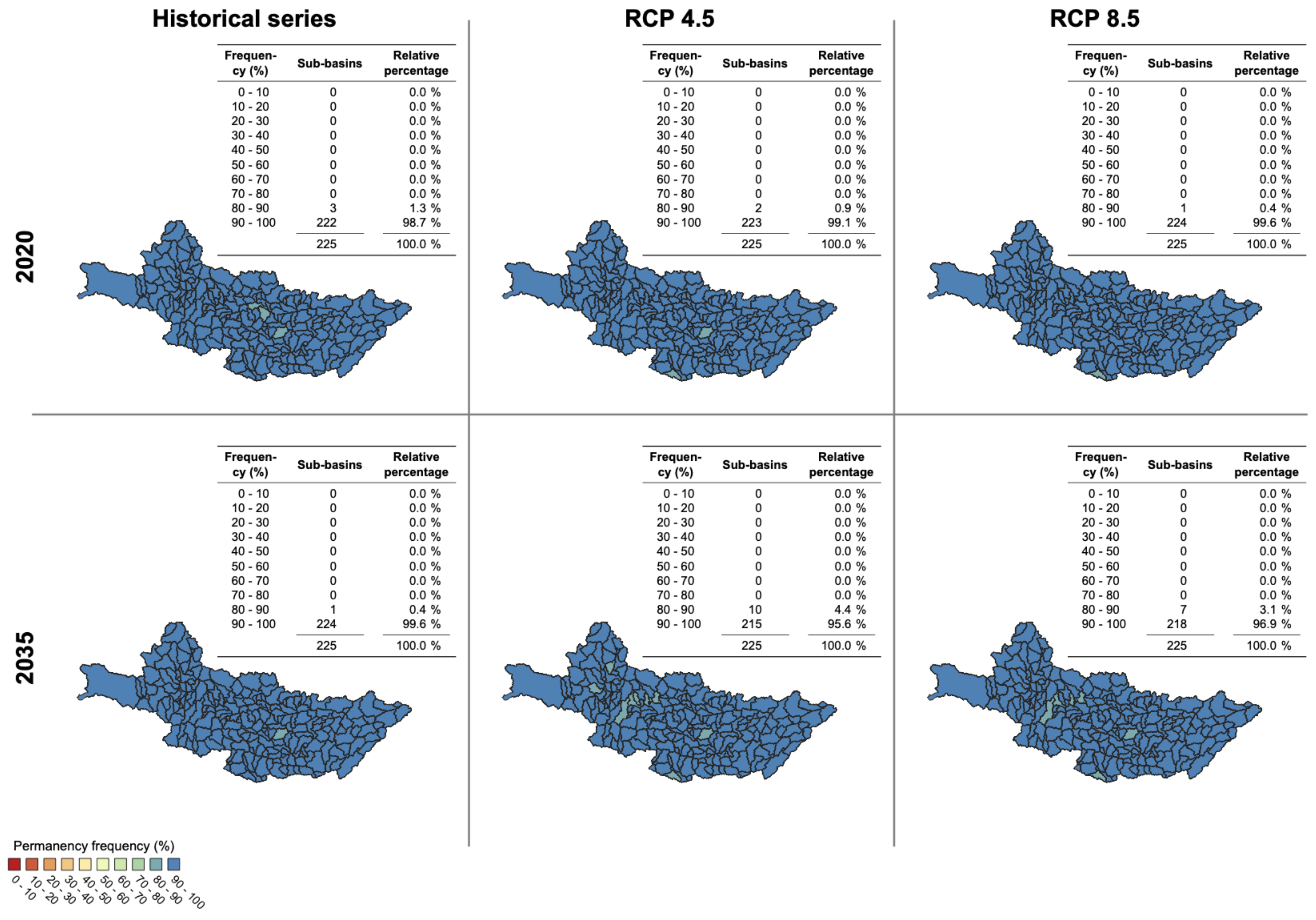
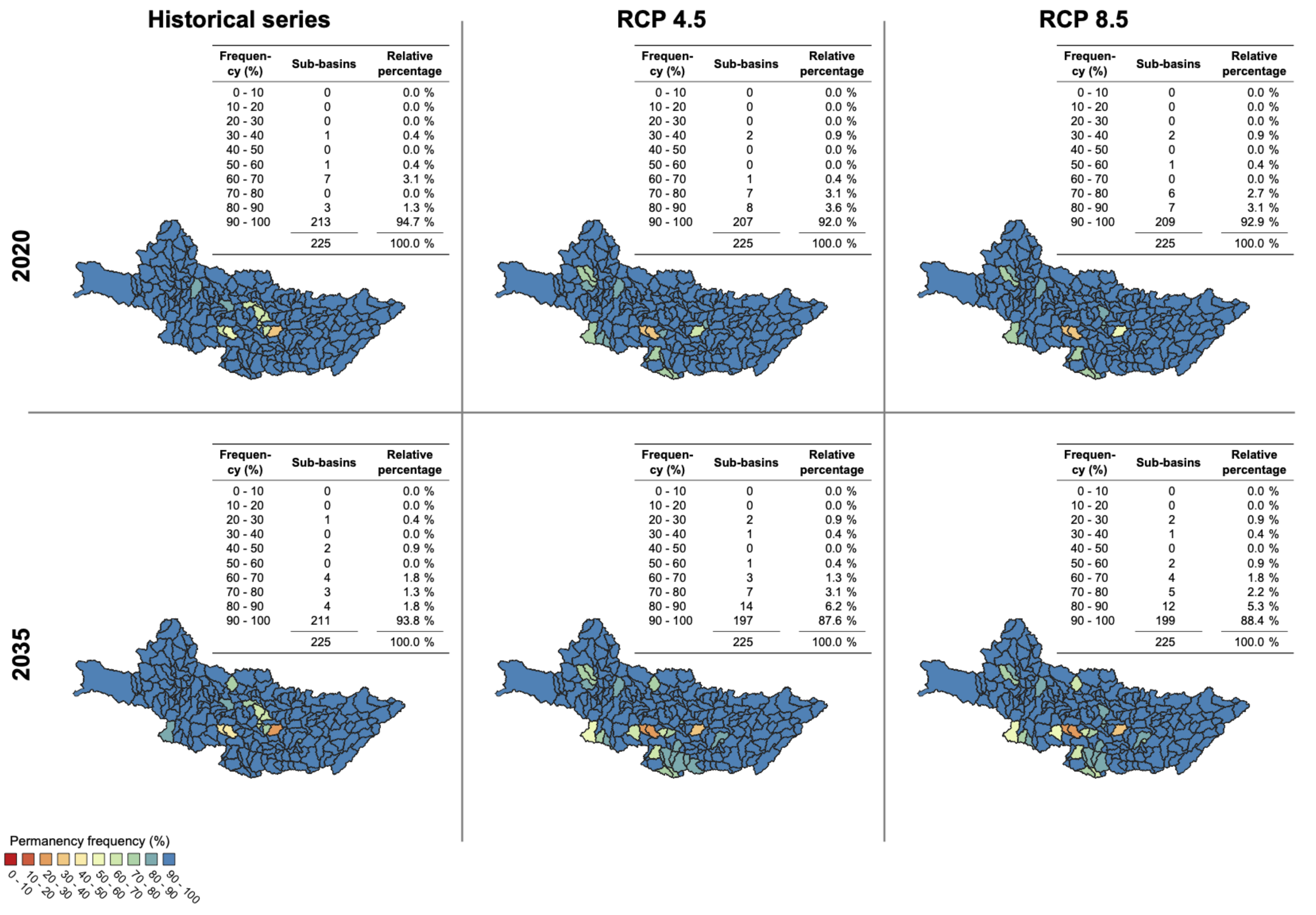
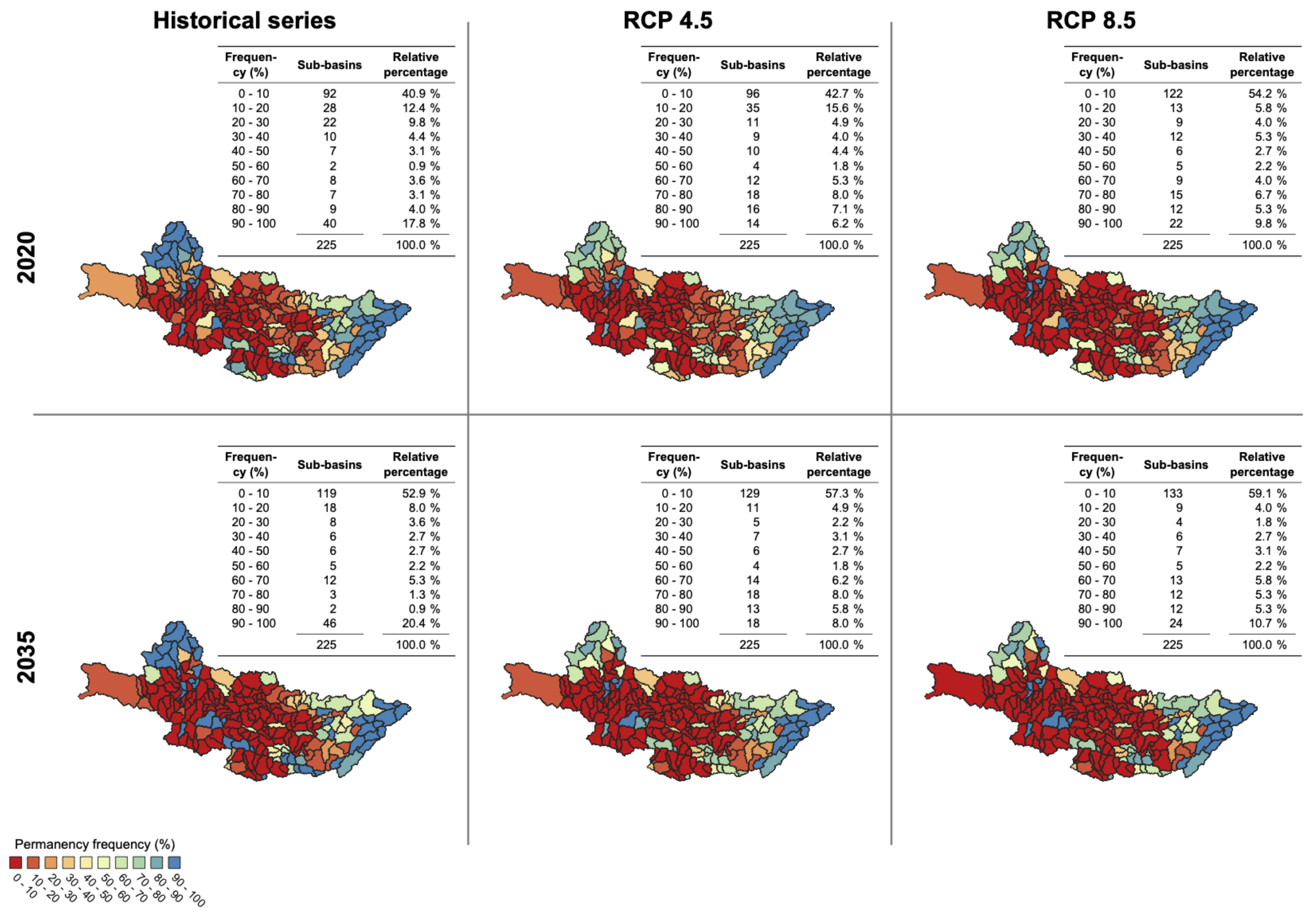
3. Results
4. Discussion
5. Conclusions
Author Contributions
Funding
Institutional Review Board Statement
Informed Consent Statement
Data Availability Statement
Conflicts of Interest
References
- Gain, A.K.; Giupponi, C.; Wada, Y. Measuring global water security towards sustainable development goals. Environ. Res. Lett. 2016, 11, 124015. [Google Scholar] [CrossRef]
- Mishra, B.K.; Kumar, P.; Saraswat, C.; Chakraborty, S.; Gautam, A. Water Security in a Changing Environment: Concept, Challenges and Solutions. Water 2021, 13, 490. [Google Scholar] [CrossRef]
- Lund, J.R. Integrating social and physical sciences in water management. Water Resour. Res. 2015, 51, 5905–5918. [Google Scholar] [CrossRef]
- Sordo-Ward, Á.; Granados, I.; Martín-Carrasco, F.; Garrote, L. Impact of Hydrological Uncertainty on Water Management Decisions. Water Resour. Manag. 2016, 30, 5535–5551. [Google Scholar] [CrossRef]
- Quesada-Montano, B.; Westerberg, I.K.; Fuentes-Andino, D.; Hidalgo, H.G.; Halldin, S. Can climate variability information constrain a hydrological model for an ungauged Costa Rican catchment? Hydrol. Process. 2018, 32, 830–846. [Google Scholar] [CrossRef]
- Dang, C.; Zhang, H.; Singh, V.P.; Yu, Y.; Shao, S. Investigating Hydrological Variability in the Wuding River Basin: Implications for Water Resources Management under the Water–Human-Coupled Environment. Water 2021, 13, 184. [Google Scholar] [CrossRef]
- Rougé, C.; Ge, Y.; Cai, X. Detecting gradual and abrupt changes in hydrological records. Adv. Water Resour. 2013, 53, 33–44. [Google Scholar] [CrossRef] [Green Version]
- Crosbie, R.S.; McCallum, J.L.; Walker, G.R.; Chiew, F.H.S. Modelling climate-change impacts on groundwater recharge in the Murray-Darling Basin, Australia. Hydrogeol. J. 2010, 18, 1639–1656. [Google Scholar] [CrossRef]
- Cui, Y.; Liao, Z.; Wei, Y.; Xu, X.; Song, Y.; Liu, H. The Response of Groundwater Level to Climate Change and Human Activities in Baotou City, China. Water 2020, 12, 1078. [Google Scholar] [CrossRef]
- Huijgevoort, M.H.J.V.; Voortman, B.R.; Rijpkema, S.; Nijhuis, K.H.S.; Witte, J.P.M. Influence of Climate and Land Use Change on the Groundwater System of the Veluwe, The Netherlands: A Historical and Future Perspective. Water 2020, 12, 2866. [Google Scholar] [CrossRef]
- Delpla, I.; Jung, A.V.; Baures, E.; Clement, M.; Thomas, O. Impacts of climate change on surface water quality in relation to drinking water production. Environ. Int. 2009, 35, 1225–1233. [Google Scholar] [CrossRef]
- Yao, Y.; Qu, W.; Lu, J.; Cheng, H.; Pang, Z.; Lei, T.; Tan, Y. Responses of Hydrological Processes under Different Shared Socioeconomic Pathway Scenarios in the Huaihe River Basin, China. Water 2021, 13, 1053. [Google Scholar] [CrossRef]
- Shiru, M.S.; Park, I. Comparison of Ensembles Projections of Rainfall from Four Bias Correction Methods over Nigeria. Water 2020, 12, 3044. [Google Scholar] [CrossRef]
- Li, X.; Zhang, L.; O’Connor, P.J.; Yan, J.; Wang, B.; Liu, D.L.; Wang, P.; Wang, Z.; Wan, L.; Li, Y. Ecosystem Services under Climate Change Impact Water Infrastructure in a Highly Forested Basin. Water 2020, 12, 2825. [Google Scholar] [CrossRef]
- Team, C.W.; Pachauri, R.K.; Meyer, L.A. (Eds.) Climate Change 2014: Synthesis Report. Contribution of Working Groups I, II and III to the Fifth Assessment Report of the Intergovernmental Panel on Climate Change; IPCC: Geneva, Switzerland, 2014. [Google Scholar]
- Mahmoud, M.; Liu, Y.; Hartmann, H.; Stewart, S.; Wagener, T.; Semmens, D.; Stewart, R.; Gupta, H.; Dominguez, D.; Dominguez, F.; et al. A formal framework for scenario development in support of environmental decision-making. Environ. Model. Softw. 2009, 24, 798–808. [Google Scholar] [CrossRef]
- Ahmadi, A.; Kerachian, R.; Skardi, M.J.E.; Abdolhay, A. A stakeholder-based decision support system to manage water resources. J. Hydrol. 2020, 589, 125138. [Google Scholar] [CrossRef]
- Gourbesville, P. Integrated river basin management, ICT and DSS: Challenges and needs. Phys. Chem. Earth Parts A/B/C 2008, 33, 312–321. [Google Scholar] [CrossRef]
- Fan, M.; Xu, J.; Chen, Y.; Li, D.; Tian, S. How to Sustainably Use Water Resources—A Case Study for Decision Support on the Water Utilization of Xinjiang, China. Water 2020, 12, 3564. [Google Scholar] [CrossRef]
- Profill-Rhama, C. Plano de Recursos Hídricos das Bacias Hidrográficas dos Rios Piracicaba, Capivari e Jundiaí, 2020 a 2035: Relatório síntese. Technical Report. 2020. Available online: https://plano.agencia.baciaspcj.org.br (accessed on 20 October 2021).
- Alvares, C.A.; Stape, J.L.; Sentelhas, P.C.; de Moraes Gonçalves, J.L.; Sparovek, G. Köppen’s climate classification map for Brazil. Meteorol. Z. 2013, 22, 711–728. [Google Scholar] [CrossRef]
- Chou, S.C.; Lyra, A.; Mourao, C.; Dereczynski, C.; Pilotto, I.; Gomes, J.; Bustamante, J.; Tavares, P.; Silva, A.; Rodrigues, D.; et al. Assessment of Climate Change over South America under RCP 4.5 and 8.5 Downscalling Scenarios. Am. J. Clim. Chang. 2014, 3, 512–525. [Google Scholar] [CrossRef] [Green Version]
- Chou, S.C.; Lyra, A.; Mourao, C.; Dereczynski, C.; Pilotto, I.; Gomes, J.; Bustamante, J.; Tavares, P.; Silva, A.; Rodrigues, D.; et al. Evaluation of the Eta Simulations Nested in Three Global Climate Models. Am. J. Clim. Chang. 2014, 3, 438–454. [Google Scholar] [CrossRef] [Green Version]
- Wang, C.; Zhang, L.; Lee, S.K.; Wu, L.; Mechoso, C.R. A global perspective on CMIP5 climate model biases. Nat. Clim. Chang. 2014, 4, 201–205. [Google Scholar] [CrossRef]
- Li, J.L.F.; Xu, K.M.; Richardson, M.; Lee, W.L.; Jiang, J.H.; Yu, J.Y.; Wang, Y.H.; Fetzer, E.; Wang, L.C.; Stephens, G.; et al. Annual and seasonal mean tropical and subtropical precipitation bias in CMIP5 and CMIP6 models. Environ. Res. Lett. 2020, 15, 124068. [Google Scholar] [CrossRef]
- Wood, A.W.; Leung, L.R.; Sridhar, V.; Lettenmaier, D.P. Hydrologic Implications of Dynamical and Statistical Approaches to Downscaling Climate Model Outputs. Clim. Chang. 2004, 62, 189–216. [Google Scholar] [CrossRef]
- Li, H.; Sheffield, J.; Wood, E.F. Bias correction of monthly precipitation and temperature fields from Intergovernmental Panel on Climate Change AR4 models using equidistant quantile matching. J. Geophys. Res. Atmos. 2010, 115. [Google Scholar] [CrossRef]
- da Silva Silveira, C.; Costa, A.A.; Coutinho, M.M.; de Assis de Souza Filho, F.; das Chagas Vasconcelos Júnior, F.; Noronha, A.W. Verificação das previsões de tempo para precipitação usando ensemble regional para o estado do Ceará em 2009. Revista Brasileira de Recursos Hídricos. 2011, 26, 609–618. [Google Scholar] [CrossRef]
- Cannon, A.J.; Sobie, S.R.; Murdock, T.Q. Bias Correction of GCM Precipitation by Quantile Mapping: How Well Do Methods Preserve Changes in Quantiles and Extremes? J. Clim. 2015, 28, 6938–6959. [Google Scholar] [CrossRef]
- Schardong, A.; Simonovic, S.P.; Gaur, A.; Sandink, D. Web-Based Tool for the Development of Intensity Duration Frequency Curves under Changing Climate at Gauged and Ungauged Locations. Water 2020, 12, 1243. [Google Scholar] [CrossRef]
- Che, D.; Mays, L.W. Development of an Optimization/Simulation Model for Real-Time Flood-Control Operation of River-Reservoirs Systems. Water Resour. Manag. 2015, 29, 3987–4005. [Google Scholar] [CrossRef]
- Shenava, N.; Shourian, M. Optimal Reservoir Operation with Water Supply Enhancement and Flood Mitigation Objectives Using an Optimization-Simulation Approach. Water Resour. Manag. 2018, 32, 4393–4407. [Google Scholar] [CrossRef]
- Brasileiro, C.N. Lei No 9433, que Institui a Política Nacional de Recursos Hídricos. Brasília, Brazil. 1997. Available online: http://www.planalto.gov.br (accessed on 20 October 2021).
- CONAMA. Resolução No 357, sobre a classificação dos Corpos d’água e Diretrizes Ambientais Para o seu Enquadramento. Brasília, Brazil. 2005. Available online: http://conama.mma.gov.br (accessed on 20 October 2021).
- de Andrade Costa, D.; da Silva Junior, L.C.S.; de Azevedo, J.P.S.; dos Santos, M.A.; dos Santos Facchetti Vinhaes Assumpção, R. From Monitoring and Modeling to Management: How to Improve Water Quality in Brazilian Rivers? A Case Study: Piabanha River Watershed. Water 2021, 13, 176. [Google Scholar]
- Knaesel, K.M.; Pinheiro, A.; Venzon, P.T.; Kaufmann, V. Scenarios of water quality management in watershed with distributed spatio-temporal simulation. Braz. J. Water Resour. 2020, 25. [Google Scholar] [CrossRef] [Green Version]
- Torres, C.; Medeiros, Y.; Freitas, I. Training watershed committee members to aid on the decision-making process for the execution program of the framework of water bodies. Braz. J. Water Resour. 2016, 21, 314–327. [Google Scholar] [CrossRef]
- Calmon, A.; Souza, J.; Reis, J.; Mendonça, A. Uso combinado de curvas de permanência de qualidade e modelagem da autodepuração como ferramenta para suporte ao processo de enquadramento de cursos d’agua superficiais. Braz. J. Water Resour. 2016, 21, 118–133. [Google Scholar] [CrossRef]


| Parameter | Unit | Class | |||
|---|---|---|---|---|---|
| 1 | 2 | 3 | 4 | ||
| DO | mg/L O2 | ⩾6.0 | ⩾5.0 | ⩾4.0 | <4.0 |
| BOD | mg/L O2 | ⩽3.0 | ⩾5.0 | ⩽10.0 | >10.0 |
| Nitrite | mg/L NO2− | ⩽1.0 | ⩽1.0 | ⩽1.0 | > 1.0 |
| Nitrate | mg/L NO3− | ⩽10.0 | ⩽10.0 | ⩽10.0 | >10.0 |
| Phosphorus | mg/L P | ⩽0.1 | ⩽0.1 | ⩽0.15 | − |
| Water Uses Projections | Without Climate Change | With Climate Change | |
|---|---|---|---|
| Historical Series (1940–1970) | RCP 4.5 (2040–2070) | RCP 8.5 (2040–2070) | |
| 2020 | Scenario 1 | Scenario 3 | Scenario 5 |
| 2035 | Scenario 2 | Scenario 4 | Scenario 6 |
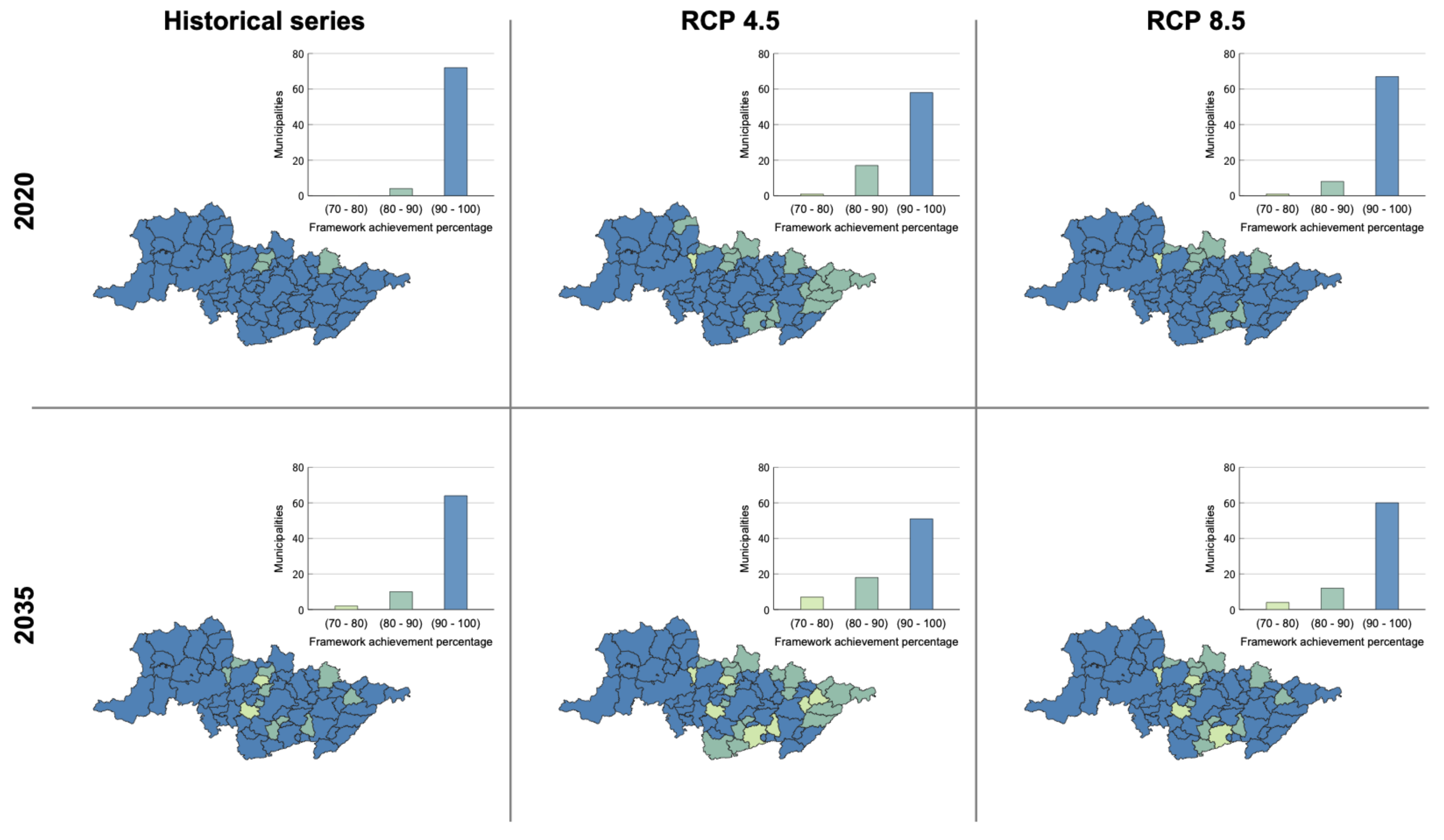
| Year | Data Series | Attendance Range (%) | Total Outflows (L/s) | Total Deficit (%) | |||
|---|---|---|---|---|---|---|---|
| (70–80) | (80–90) | (90–100) | Demanded | Delivered | |||
| 2020 | Historical | 0 | 4 | 72 | 30,508 | 29,736 | 2.53 |
| RCP 4.5 | 1 | 17 | 58 | 30,508 | 29,167 | 4.39 | |
| RCP 8.5 | 1 | 8 | 67 | 30,508 | 29,988 | 1.71 | |
| 2035 | Historical | 2 | 10 | 64 | 31,725 | 30,798 | 2.92 |
| RCP 4.5 | 7 | 18 | 51 | 31,725 | 30,026 | 5.35 | |
| RCP 8.5 | 4 | 12 | 60 | 31725 | 30945 | 2.46 | |

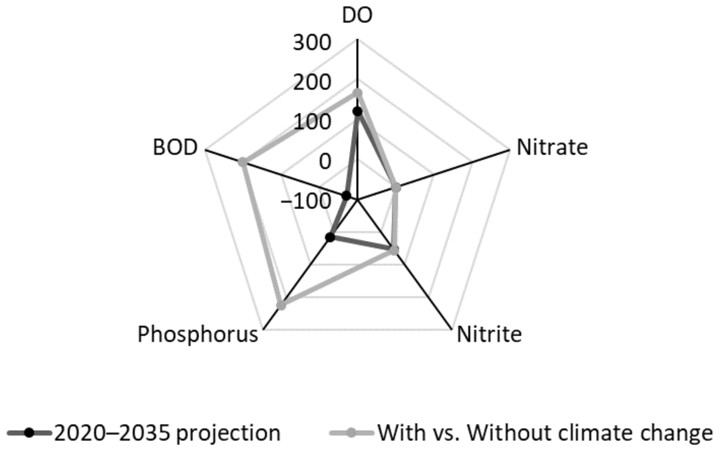
| Type | BOD | DO | Nitrate | Nitrite | Phosphorus | Index |
|---|---|---|---|---|---|---|
| 2020–2035 projection | −73.6 | 112.4 | 0.0 | 18.0 | 27.0 | a |
| −70.9 | 106.8 | 0.0 | 68.1 | 9.3 | b | |
| −69.4 | 143.6 | 0.0 | 72.7 | 11.3 | c | |
| With vs. without climate change | 229.5 | 198.4 | 0.0 | 33.8 | 264.2 | d |
| 167.5 | 121.2 | 0.0 | 26.8 | 201.7 | e | |
| 232.3 | 192.9 | 0.0 | 83.8 | 246.5 | f | |
| 171.7 | 152.4 | 0.0 | 81.5 | 186.0 | g | |
Publisher’s Note: MDPI stays neutral with regard to jurisdictional claims in published maps and institutional affiliations. |
© 2021 by the authors. Licensee MDPI, Basel, Switzerland. This article is an open access article distributed under the terms and conditions of the Creative Commons Attribution (CC BY) license (https://creativecommons.org/licenses/by/4.0/).
Share and Cite
Tercini, J.R.B.; Perez, R.F.; Schardong, A.; Bonnecarrère, J.I.G. Potential Impact of Climate Change Analysis on the Management of Water Resources under Stressed Quantity and Quality Scenarios. Water 2021, 13, 2984. https://doi.org/10.3390/w13212984
Tercini JRB, Perez RF, Schardong A, Bonnecarrère JIG. Potential Impact of Climate Change Analysis on the Management of Water Resources under Stressed Quantity and Quality Scenarios. Water. 2021; 13(21):2984. https://doi.org/10.3390/w13212984
Chicago/Turabian StyleTercini, João Rafael Bergamaschi, Raphael Ferreira Perez, André Schardong, and Joaquin Ignacio Garcia Bonnecarrère. 2021. "Potential Impact of Climate Change Analysis on the Management of Water Resources under Stressed Quantity and Quality Scenarios" Water 13, no. 21: 2984. https://doi.org/10.3390/w13212984