Physics of Traveling Waves in Shallow Water Environment

Abstract

We present a study of the physical characteristics of traveling waves at shallow and intermediate water depths. The main subject of study is to the influence of nonlinearity on the dispersion properties of waves, their limiting heights and steepness, the shape of solitary waves, etc. A fully nonlinear Serre–Green–Naghdi-type model, a classical weakly nonlinear Boussinesq model and fifth-order Stokes wave solutions were chosen as models for comparison. The analysis showed significant, if not critical, differences in the effect of nonlinearity on the properties of traveling waves for these models. A comparison with experiments was carried out on the basis of the results of a joint Russian–Taiwanese experiment, which was carried out in 2015 at the Tainan Hydraulic Laboratory, and on available experimental data. A comparison with the experimental results confirms the applicability of a completely nonlinear model for calculating traveling waves over the entire range of applicability of the model in contrast to the Boussinesq model, which shows contradictory and unrealistic wave properties for moderate wavelengths.

1. Introduction

Long water wave research has a history of more than two hundred years. The high suitability of shallow water theories for various practical problems is still of unremitting interest. The two classical Korteweg and de Vries (KDV) [1] and Boussinesq models (BM) [2], together with the nonlinear Airy wave theory [3], laid the foundation for the study of waves in shallow water. Cnoidal traveling waves, which are solutions to the equations of KDV and BM, have been detailed and presented in an easy-to-use form by Wiegel et al. [4,5]. The main physical characteristics of waves, such as period and wavelength, celerity, phase speed and other properties, were presented in visible and tabular form. An experimental study of cnoidal waves in shoaling water was presented in [6].

Long waves are usually characterized by a small “shallowness” parameter $\sigma =d/L$; the ratio of water depth d to the typical wave length L; and an amplitude parameter $\epsilon =a/d$, where a is the wave amplitude, which expresses the ratio of wave amplitude to calm-water depth. Asymptotic expansions of the Euler equations for the motion of an ideal fluid in these two small parameters of different orders have led to an endless stream of wave models on shallow and intermediate water up to present time [7,8].

A strong impetus in the development of the theory of weakly nonlinear and weakly dispersive waves was made in the second half of the twentieth century in the work by Peregrine [9], Benjamin et al. [10], Degasperith et al. [11], Su and Gardner [12], and many others. A whole series of extended Boussinesq-type models have been proposed, which provide an accurate description of wave processes in a wider range of wave depths and amplitudes than the classical Boussinesq model [13,14,15,16,17,18]. The list of significant works on this topic is unimaginably large and it is impossible to display it in full, so we limited ourselves to citing the work most similar to our study.

One way to assess the “quality” of approximate models is to compare their linear dispersion properties with linearized solutions of the full Euler equations. Classical (KDV) and (BM) linearized equations adequately reproduced dispersion properties of the Euler equations only for very long waves with wavenumbers closed to zero. Whitham [19] presented the equation for water waves, which reproduce the dispersion relation for all lengths of waves. Many models have been proposed with improved linearized dispersion properties [20,21,22,23]. One way to expand the scope (BM) is to introduce a free parameter into the model and to select it appropriately to improve its linear dispersion properties [20,21]. Nwogu [22] introduced a free parameter that uses speed calculated at an arbitrary depth as a reference speed instead of a depth-averaged speed. Schaffer [24], and Karambas and Memos [25] proposed Boussinesq-type equations with exact linear dispersion properties, but despite their improved dispersion relation, the equations were still restricted to weakly nonlinear waves. It can be noted that, in general, scientific research is more concentrated on various linear properties of models, although they are intended for the analysis of nonlinear waves.

A thorough comparison of the various approximate models must account for nonlinear effects. Fully nonlinear Serre–Green–Naghdi (SGN) equations that can describe the propagation of large-amplitude waves were derived by Serre [26]; by Su and Gardner [12]; and then by Green, Laws and Naghdi [27]. These weakly dispersive equations include all terms up to the third order of expansion in the small shallowness parameter σ. These SGN equations represent a significant improvement over Boussinesq’s theory. Several extended SGN-type models have recently been proposed, and their mathematical properties have been studied [28,29,30]. The models improved the linearized dispersion properties, but did not fulfill the energy conservation law. Consistent, modified SGN equations that conserve both energy and momentum were recently proposed by Clamond, Dutykh and Mitsotakis [31]. Experimental studies on this issue were recently presented in [32,33]

Important classes of solutions that include the full nonlinear effects are the so-called periodic in space cnoidal traveling waves, i.e., the wave profiles propagating with a constant speed without changing their form. In the literature on wave motions of a liquid at shallow and intermediate water depths, one can often find the term “cnoidal” waves with self-implied physical properties, a region of existence and stability. This terminology seems to not be entirely justified due to the fact that wave solutions in the form of cnoidal functions appearing in a huge number of models can have significantly different physical properties.

The aim of the present study is to describe the physical properties of traveling wave solutions for completely nonlinear wave models of the SGN type and to compare them with weakly nonlinear solutions using the example of Boussinesq (BM) theory. We also present the results of calculations using the improved SGN model [31] and fifth-order Stokes wave solutions for intermediate water depths [34,35].

A comparison with experiments is carried out on the basis of the results of a joint Russian–Taiwanese experiment, which was carried out in 2015 at the Tainan Hydraulic Laboratory of the National Cheng-Kung University, and on the data presented by Wiegel [4,6].

We try to point out some important particularities of traveling waves that have not attracted as much attention from researchers.

This article is organized as follows. In Section 2, we briefly present the strongly nonlinear SGN model (FN) and improved SGN model (iFN) and present its traveling wave solutions (details are given in the Appendix A). Section 3 describes the main physical properties of traveling waves for the FN, iFN and Stokes models in comparison with the classical Boussinesq model (BM) and some experimental data:

-

Solitary waves (Section 3.1);

-

Nonlinear dispersion relation (Section 3.2);

-

Wave steepness characteristic of waves (Section 3.3);

-

Comparison with experiments (Section 3.4); and

-

Region of existing of the traveling waves (Section 3.5).

Conclusions are made in Section 4.

2. Basic Equations of Motion and Traveling Solutions

Consider a horizontal layer of an ideal incompressible homogeneous fluid with a free surface. Two-dimensional Cartesian coordinates (x, z) are represented by the horizontal x-axis and the z-axis pointed vertically upward. A flat impermeable bottom is given by z = 0, and surface tension effects are ignored. The fluid flow is described by the vertically averaged velocity of fluid $\overline{u}=1/h{\displaystyle \underset{0}{\overset{h}{\int }}udz}$, where $u$ is the horizontal velocity component, free surface elevation $h=d+\eta (x,t)$ and d is the still-water level.

We use several theoretical models of wave motion for comparison: the classical weakly nonlinear Boussinesq model (BM), the strongly nonlinear Serre–Green–Naghdi (FN) model, an improved SGN model (iFN) and fifth-order Stokes wave solutions for intermediate water depths.

Dimensionless equations (FN) have the following form:

$$\{\begin{array}{l}{h}_t+(\overline{u}h{)}_x=0\\ {\overline{u}}_t+\overline{u}{\overline{u}}_x+h_x=1/(3h)({\overline{u}}_{xt}+\overline{u}{\overline{u}}_{xx}-{\overline{u}}_x^2{)}_x\end{array}$$

(1)

The derivation of these equations in detail is given in Appendix A.

The classical Boussinesq equations (BM) can be obtained by linearizing the right-hand side of the momentum Equation in (1).

The improved SGN set of equations (iFN) have the following form:

$$\{\begin{array}{l}{h}_t+(\overline{u}h{)}_x=0,\\ q_t+{\left[\overline{u}q-\frac{1}{2}{\overline{u}}^2+h-\left(\frac{1}{2}+\frac{3}{4}\beta \right)h^2{\overline{u}}_x^2-\frac{1}{2}\beta (h^2{h}_{xx}+h{h}_x^2)\right]}_x=0,\end{array}$$

where $q=\overline{u}-(1/3+\beta /2)h^{-1}{[h^3{\overline{u}}_x]}_x$. This system contains a free parameter $\beta$, which is chosen to provide a better fit for the dispersion of the complete Euler equations for infinitely small amplitudes: $\beta =2/15$.

We analyze solutions of the traveling wave type assuming that all unknown functions depend on a single coordinate $\xi =x-ct$, where c is the velocity of the reference frame in which the waves are stationary. The solutions of the BM and FN models in the form of periodic traveling waves for the elevation of the free surface $\eta (\xi )$ can be parametrically expressed in terms of cnoidal functions:

$$\eta ={\eta }_{tr}+HC{n}^2\left[\frac{2K(m)}{L}\xi \right]$$

where $({\eta }_{tr},{\eta }_{cr})$ are the trough and crest elevations; ($H={\eta }_{cr}-{\eta }_{tr}$, L) are the wave height and length, respectively; $Cn[z,m]$ is the cosine-elliptic function with the parametric modulus m; and $K[m]$ is the complete elliptic integral of the first kind. The details of this solution are given in the Appendix A.

3. Results

The nonlinear properties of traveling waves not only are manifested in the form of profiles of such waves but also are primarily characterized by their nonlinear dispersion characteristics and, in particular, by the dependence of their phase velocity on the wavelength and height of the waves. We carry out a comparative analysis of these properties for various wave motion models for shallow and intermediate water depths. We present the main characteristics of highly nonlinear traveling waves (FN) in comparison with classical Boussinesq (BM) solutions. Both theories describe traveling waves in terms of periodic cnoidal functions, but their dispersion characteristics can differ significantly. We also present the results of calculations using the improved SGN model (iFN) and fifth-order Stokes wave (SW) solutions for intermediate water depths [34,35].

A comparison with experiments is carried out on the basis of the results of a joint Russian–Taiwanese experiment, which was carried out in 2015 at the Tainan Hydraulic Laboratory of the National Cheng-Kung University, and data on provided by Wiegel [4,6].

3.1. Solitary Waves

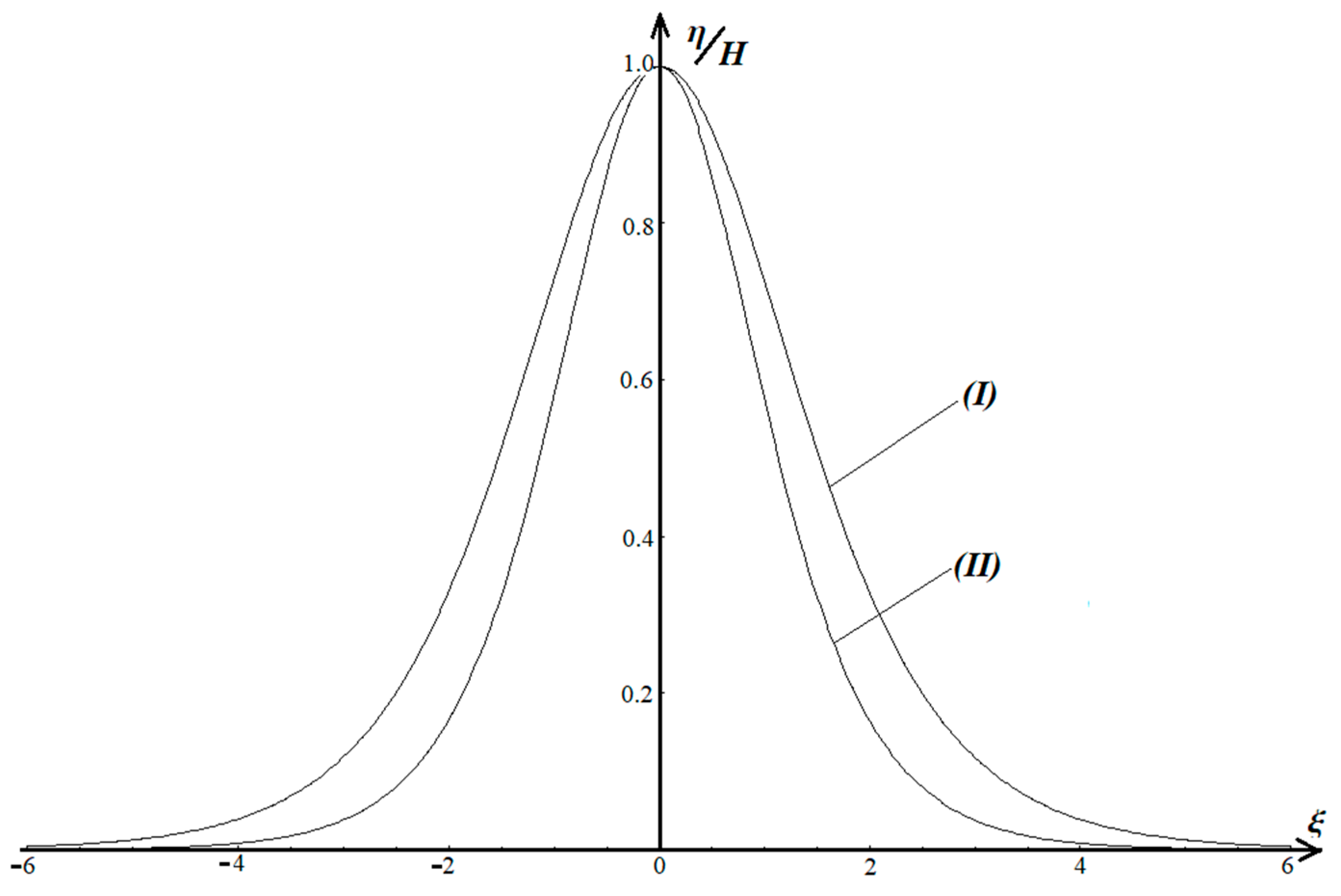
In the very long wave limit, the elliptic parameter $m\to 1$ and the solitary wave solution is

$$\varsigma =H\sec h^2\left(\frac{\xi }{\mathsf{\Delta }}\right)$$

(2)

where $\mathsf{\Delta }$ is the so-called solitary wave width, which is different for the (FN) and (BM) models:

$$\mathsf{\Delta }=\sqrt{\frac{4}{3H}}\mathrm{for}\left(\mathrm{BM}\right),$$

$$\mathsf{\Delta }=\sqrt{\frac{4(H+1)}{3H}}\mathrm{for}\left(\mathrm{FN}\right).$$

The profile of both solitary waves is shown in Figure 1 for H = 0.8. The solitary wave profile is surprisingly gentler for the FN model and less dependent on wave height.

3.2. Nonlinear Dispersion Relation

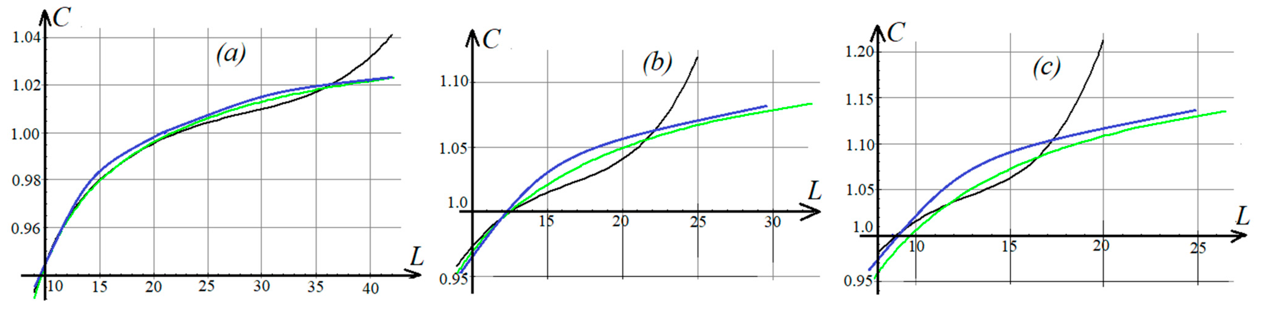
The dependences of the phase velocity C of waves on the length L for different wave heights H for the FN, iFN and SW models are shown in Figure 2. All models show the best, almost identical coincidence for low wave heights (Figure 2a) in almost the entire significant wavelength interval. The Stokes model is unable to adequately describe only very long quasi-solitary waves. Both highly nonlinear wave models show good mutual agreement for all considered wave heights. The improved SGN model (iFN) gives slightly increased values of phase velocities in comparison with the FN model. The range of applicability of the Stokes model strongly decreases with wave height and is located in the region of intermediate water depths. This is easily explained by the weakly nonlinear nature of the model, which was obtained for deep and intermediate water depths.

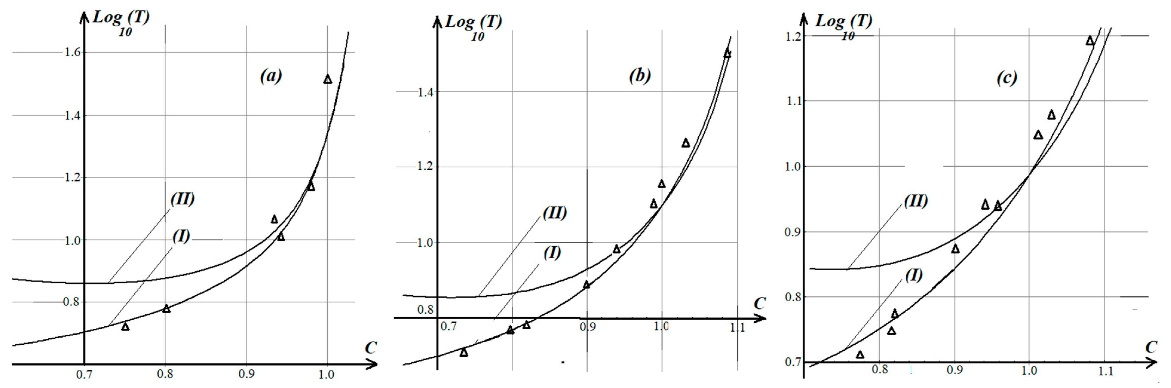
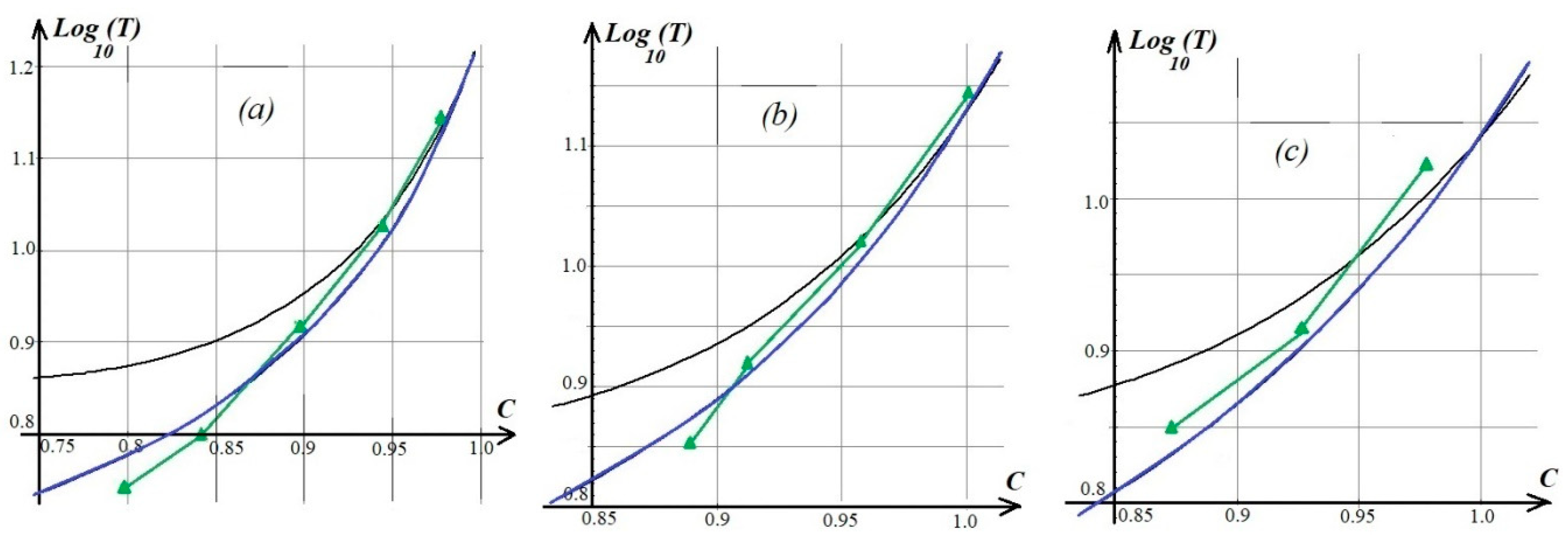
The phase velocity versus wave period for the FN and BM models, and the experimental data [6] are compared in Figure 3. An acceptable agreement between the two models can only be seen for sufficiently long wave periods. For moderate wave periods, the phase velocity is significantly lower than that predicted by the weakly nonlinear (BM) theory. The fully nonlinear model (PM) demonstrates much better agreement with the experimental results over the entire range of wave periods.

3.3. Nonlinear Wave Steepness

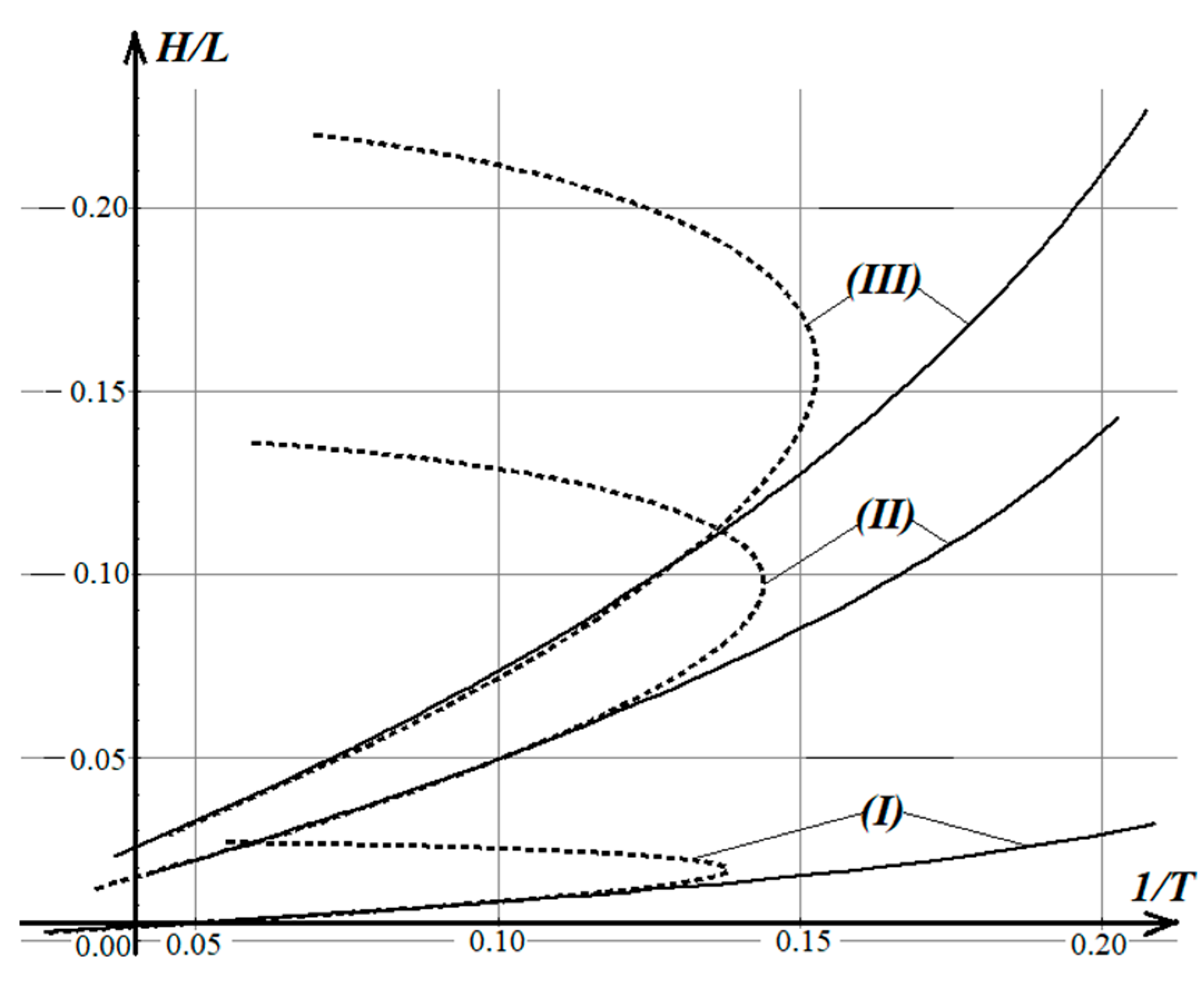
The dependence of the wave steepness (H/L) on the period T for different wave heights H for the FN and BM models is shown in Figure 4.

Here, you can see a fundamental difference in the theoretical results for the two models: the BM model is generally unable to describe the wave steepness for moderate wave periods, while the FN model gives reasonable results. Moreover, BM shows conflicting results: for the same period and wave height, there are two different wavelengths. This once again emphasizes the ‘weakness’ of weakly nonlinear theories when describing waves at an intermediate water depth.

3.4. Comparison with Experiments in Tainan Hydraulics Laboratory

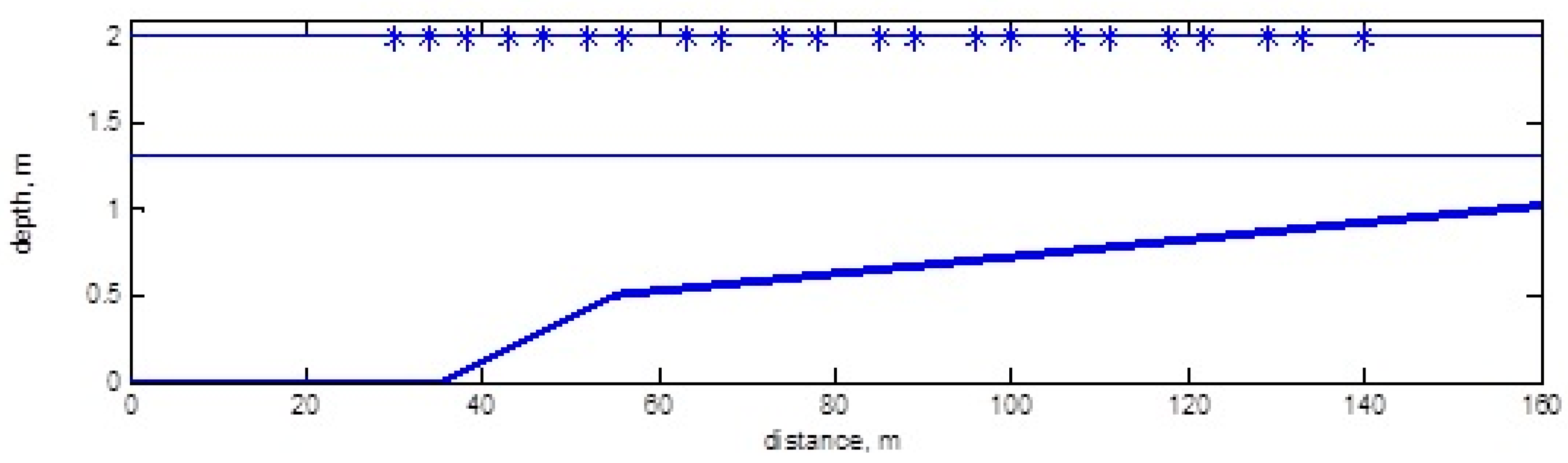
To compare the FN and BM predictions for the phase velocities with the physical experimental results, we use the data from a joint Russian–Taiwan experiment that was performed in 2015 at the medium wave flume of Tainan Hydraulic Laboratory of National Cheng-Kung University. The flume is 200 m long, 2 m in wide and 2 m in depth. At the beginning, the flume was the piston-type fully programmable controlling wave mare; at the end, the flume was the wave absorber constructed by small rocks and synthetic nets. The bottom was horizontal for the first 30 m, then inclined by 1/40 at the next 20 m and then inclined by 1/200 up to the shore. During the experiments, the still water-level over the horizontal part of bottom was 1.27 m. During the experiment, 21 capacitance-type wire wave gauges were installed spaced by 4 or 7 m from each other, as shown in Figure 5, and acquired synchronously by a 50 Hz sampling rate. For this paper, we use only the gauges installed at the first 30 m of the flume and the wave regimes of initially monochromatic waves with height 20 cm in wave period ranges 1 to 4 s.

Phase velocities c were measured by finding the maximum of the cross-correlation function at adjacent measurement points. Furthermore, it was calculated as $c=L/\tau$, where L is the distance between adjacent measurement points and $\tau$ is the delay in the maximum of the cross-correlation function.

The errors from determining the phase velocity were estimated by the full differential method:

$$\delta c=\delta \left(\frac{L}{\tau }\right)=\frac{\tau \delta L+L\delta \tau }{{\tau }^2}$$

We estimate the typical values of $\delta \tau =0.02\sec$ as a step in the free surface elevation discretization, $\tau =1.2\sec$ is the typical time delay for a distance of 4 m, $\delta L=2\mathrm{cm}$ is the error in the wave gauge positioning and L = 4 м. Therefore, the error of c estimations is $\delta c=0.07\mathrm{m}/\sec$.

The wave period versus phase velocity for the FN and BM models, and our experimental results are compared in Figure 6.

The best agreement with the experiment was shown by calculations using the FN model for relatively small wave heights (Figure 6a). With increasing heights, the FN model gives slightly overestimated values of phase velocities. The BM model is unable to adequately describe waves with moderate periods. In general, the strongly nonlinear model (FN) shows much better agreement with the experimental results compared with the Boussinesq model over the entire range of wave periods.

3.5. The Region of Existence of Traveling Waves

A necessary criterion for existing traveling wave solutions based on the non-local formulation of the Euler full water wave problem for finite and infinite water depths [36] was recently obtained in [37,38]. The amplitude of waves is limited by their propagation speed:

$${\eta }_{cr}\le c^2/2$$

(3)

It is quite interesting to apply this criterion to shallow water wave models. The last inequality can be expressed in terms of the parameter m of the cnoidal functions and the wave height H:

$$H\le \frac{m}{m+E(m)/K(m)}$$

(4)

The region of existing traveling wave solutions in the context of a shallow water environment is shown in Figure 7 as a shadow zone in the plane (H, C). The limiting values here ($H=1,c=\sqrt{2}$) correspond to solitary waves.

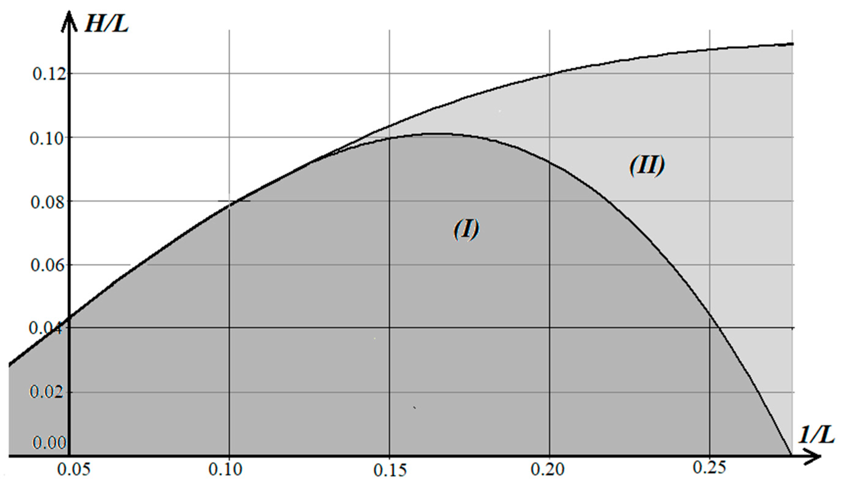
Zones of permissible wave steepness versus wavelength are shown in Figure 8 for the FN and BM models. The shadow zone (I) corresponds to the model BM, and the shadow zones (I) plus (II) correspond to a fully nonlinear model (FN). As can be seen, the admissible regions for the two models are fundamentally different for moderate wavelengths. The BM model appears to express unrealistically low steepness values for moderate wavelengths.

4. Conclusions

Nonlinearity plays a decisive role in determining the physical characteristics of traveling waves at shallow and intermediate water depths. The phase velocity of traveling waves increases significantly with increasing wave amplitude. We present the dispersion properties of highly nonlinear traveling waves (FN) in comparison with classical Boussinesq (BM) solutions. We also present the results of calculations using the improved SGN model (iFN) and fifth-order Stokes wave (SW) solutions for intermediate water depths. The dependences of the phase velocity of waves on the length for the FN, iFN and SW models show almost identical coincidence for low wave heights in almost the entire significant wavelength interval. The Stokes model is unable to adequately describe only very long quasi-solitary waves. Both highly nonlinear wave models show good mutual agreement for all considered wave heights. The improved SGN model (iFN) gives slightly increased values of phase velocities in comparison with the (FN) model. The range of applicability of the Stokes model strongly decreases with wave height and is located in the region of intermediate water depths. A comparison with experiments was carried out on the basis of the results of a joint Russian–Taiwanese experiment, which was carried out in 2015 at the Tainan Hydraulic Laboratory of the National Cheng-Kung University, and on data provided by Wiegel. The strongly nonlinear model (FN) demonstrates much better agreement with the experimental results over the entire range of wave periods. The completely nonlinear model of waves adequately describes the nonlinear dispersion properties of waves for different wave heights in contrast with the classical Boussinesq model, which shows its inappropriateness for describing waves at an intermediate water depth. The criteria for the existence of traveling wave solutions make it possible to realistically estimate their limiting height and steepness.

References

- Korteweg, D.J.; De Vries, G. On the Change of Form of Long Waves Advancing in a Rectangular Canal and On a New Type of Long Stationary Waves. Phil. Mag. 1895, 39, 422–443. [Google Scholar] [CrossRef]
- Boussinesq, J. Theorie de L’Intuumescence Liquide Appelee Onde Solitaire ou de Translation. Comtes Rendus Acad. Sci. Paris 1871, 72, 755–759. [Google Scholar]
- Stoker, J.J. Water Waves; Interscience: New York, NY, USA, 1957. [Google Scholar]
- Wiegel, R.L. A presentation of cnoidal wave theory for practical application. J. Fluid Mech. 1960, 7, 273–286. [Google Scholar] [CrossRef] [Green Version]
- Masch, F.D.; Wiegel, R.L. Cnoidal Waves—Tables of Functions; Council on Wave Research, The Engineering Foundation: Richmond, CA, USA, 1961; p. 129. [Google Scholar]
- Wiegel, R.L. Experimental study of surface waves in shoaling water. Trans. Am. Geoph. Union. 1950, 31, 377–385. [Google Scholar] [CrossRef]
- Constantin, A.; Johnson, R.S. On the Non-Dimensionalisation, Scaling and Resulting Interpretation of the Classical Governing Equations for Water Waves. J. Nonlinear Math. Phys. 2008, 15, 58–73. [Google Scholar] [CrossRef] [Green Version]
- Johnson, R.S. Camassa–Holm, Korteweg–de Vries and related models for water waves. J. Fluid Mech. 2002, 455, 63–82. [Google Scholar] [CrossRef]
- Peregrine, D.H. Long waves on a beach. J. Fluid Mech. 1967, 27, 815–827. [Google Scholar] [CrossRef]
- Benjamin, T.B.; Bona, J.L.; Mahoney, J.J. Model equations for long waves in nonlinear dispersive systems. Phil. Trans. R. Soc. Lond. Ser. A Math. Phys. Eng. Sci. 1972, 227, 47–78. [Google Scholar]
- Degasperis, A.; Holm, D.D.; Hone, A.N.W. A new integrable equation with peakon solutions. Theor. Math. Phys. 2002, 133, 1463–1474. [Google Scholar] [CrossRef] [Green Version]
- Su, C.H.; Gardner, C.S. Korteweg-de Vries equation and generalizations. III. Derivation of the Kortewegde Vries equation and Burgers equation. J. Math. Phys. 1969, 10, 536–539. [Google Scholar] [CrossRef]
- Camassa, R.; Holm, D. An integrable shallow water equation with peaked solitons. Phys. Rev. Lett. 1993, 71, 1661–1664. [Google Scholar] [CrossRef] [Green Version]
- Degasperis, A.; Procesi, M. Asymptotic integrability. In Symmetry and Perturbation Theory; Degasperis, A., Gaeta, G., Eds.; World Scientific: Singapore, 1999; pp. 23–37. [Google Scholar]
- Agnon, Y.; Madsen, P.A.; Schaffer, H. A new approach to high order Boussinesq models. J. Fluid Mech. 1999, 399, 319–333. [Google Scholar] [CrossRef]
- Schaffer, H.A.; Madsen, P.A.; Deigaard, R.A. Boussinesq model for waves breaking in shallow water. Coast. Eng. 1993, 20, 185–202. [Google Scholar] [CrossRef]
- Madsen, P.A.; Schaffer, H.A. Higher-order Boussinesq-type equations for surface gravity waves: Derivation and analysis. Phil. Trans. R. Soc. Lond. A 1998, 356, 3123–3184. [Google Scholar] [CrossRef]
- Chen, Q.; Kirby, J.T.; Dalrymple, R.A.; Kennedy, A.B.; Chawla, A. Boussinesq modeling of wave transformation, breaking and runup. II: 2D. J. Waterw. Port Coast. Ocean Eng. 2000, 126, 48–56. [Google Scholar] [CrossRef]
- Whitham, G.B. Linear and Nonlinear Waves; Wiley: New York, NY, USA, 1999. [Google Scholar]
- Bona, J.L.; Smith, R. A model for the two-way propagation of water waves in a channel. Math. Proc. Camb. Phil. Soc. 1976, 79, 167–182. [Google Scholar] [CrossRef]
- Bona, J.L.; Chen, M.; Saut, J.-C. Boussinesq equations and other systems for small amplitude long waves in nonlinear dispersive media. I: Derivation and linear theory. J. Nonlinear Sci. 2002, 12, 283–318. [Google Scholar]
- Nwogu, O. Alternative form of Boussinesq equations for nearshore wave propagation. J. Waterw. Port Coast. Ocean Eng. 1993, 119, 618–638. [Google Scholar] [CrossRef] [Green Version]
- Madsen, P.A.; Sorensen, O.R. A new form of the Boussinesq equations with improved linear dispersion characteristics. Part 2. A slowly-varying bathymetry. Coast. Eng. 1992, 18, 183–204. [Google Scholar] [CrossRef]
- Schaffer, H.A. Another step towards a post-Boussinesq wave model. In Coastal Engineering 2004; World Scientific: Singapore, 2005; pp. 132–144. [Google Scholar]
- Karambas, T.V.; Memos, C.D. A Boussinesq model for weakly nonlinear fully dispersive water waves. J. Waterw. Port Coast. Ocean Eng. 2009, 135, 187–199. [Google Scholar] [CrossRef]
- Serre, F. Contribution à l’étude des écoulements permanents et variables dans les canaux. La Houille Blanche 1953, 8, 374–388. [Google Scholar] [CrossRef] [Green Version]
- Green, A.E.; Laws, N.; Naghdi, P.M. On the theory of water waves. Proc. R. Soc. Ser. A 1974, 338, 43–55. [Google Scholar]
- Wei, G.; Kirby, J.T.; Grilli, S.T.; Subramanya, R. A fully nonlinear Boussinesq model for surface waves. I. Highly nonlinear unsteady waves. J. Fluid Mech. 1995, 294, 71–92. [Google Scholar] [CrossRef]
- Madsen, P.A.; Bingham, H.B.; Schaffer, H.A. Boussinesq-type formulations for fully nonlinear and extremely dispersive water waves: Derivation and analysis. Proc. R. Soc. Lond. A 2003, 459, 1075–1104. [Google Scholar] [CrossRef]
- Quirchmayr, R. A new highly nonlinear shallow water wave equation. J. Evol. Equ. 2016, 16, 539–567. [Google Scholar] [CrossRef]
- Clamond, D.; Dutykh, D.; Mitsotakis, D. Conservative modified Serre-Green-Naghdi equations with improved dispersion characteristics: Improved Serre-Green-Naghdi equations. Commun. Nonlinear Sci. Numer. Simul. 2017, 45, 245–257. [Google Scholar] [CrossRef] [Green Version]
- Kuznetsov, S.; Saprykina, Y. Nonlinear Wave Transformation in Coastal Zone: Free and Bound Waves. Fluids 2021, 6, 347. [Google Scholar] [CrossRef]
- Saprykina, Y.V.; Kuznetsov, S.Y.; Kuznetsova, O.A.; Shugan, I.V.; Chen, Y.Y. Wave Breaking Type as a Typical Sign of Nonlinear Wave Transformation Stage in Coastal Zone. Phys. Wave Phenom. 2020, 28, 75–82. [Google Scholar] [CrossRef]
- Fenton, J.D. A fifth-order Stokes theory for steady waves. J. Warterw. Port Coast. Ocean Eng. 1985, 111, 216–234. [Google Scholar] [CrossRef] [Green Version]
- Nishimura, H.; Isobe, M.; Horikawa, K. Higher Order Solutions of Stokes and Cnoidal Waves. J. Fac. Eng. 1977, 34, 2. [Google Scholar]
- Ablowitz, M.J.; Fokas, A.S.; Musslimani, Z.H. On a new non-local formulation of water waves. J. Fluid Mech. 2006, 562, 313–343. [Google Scholar] [CrossRef] [Green Version]
- Deconnick, B.; Oliveras, K. The instability of periodic surface gravity waves. J. Fluid Mech. 2011, 675, 141–167. [Google Scholar] [CrossRef] [Green Version]
- Craig, W.; Sternberg, P. Symmetry of solitary waves. Commun. Partial. Differ. Equ. 1988, 13, 603–633. [Google Scholar] [CrossRef]
Figure 1.
Solitary waves for H = 0.8, (I) and (II) FN and BM models, respectively.
Figure 2.
Dependence of the phase velocity C of waves on the length L for various wave heights: (a) H = 0.1, (b) H = 0.3 and (c) H = 0.5. The green, blue and black lines correspond to the FN, iFN and SW models, respectively.
Figure 3.
Dependence of the period T on the wave phase velocity C for different wave heights H: (a) H = 0.1, (b) H = 0.3 and (c) H = 0.5; (I) FN model, (II) BM model; triangles—experimental data [6].