
A Coupled Sampling Design for Parameter Estimation in Microalgae Growth Experiment: Maximizing the Benefits of Uniform and Non-Uniform Sampling


1
School of Environment, Beijing Normal University, Beijing 100875, China
2
College of Architecture and Civil Engineering, Beijing University of Technology, Beijing 100124, China
*
Author to whom correspondence should be addressed.
Water 2021, 13(21), 2996; https://doi.org/10.3390/w13212996
Submission received: 29 August 2021
/
Revised: 15 October 2021
/
Accepted: 19 October 2021
/
Published: 24 October 2021
(This article belongs to the Special Issue Interaction among Hydrological, Environmental and Ecological Processes in Aquatic Ecosystems)
Abstract
:As an important primary producer in aquatic ecosystems, the various parameters within the mathematical models are used to describe the growth of microalgae and need to be estimated by carefully designed experiments. Non-uniform sampling has proved to generate a deliberately optimized sampling temporal schedule that can benefit parameter estimation. However, the current non-uniform sampling method depends on prior knowledge of the nominal values of the model parameters. It also largely ignores the uncertainty associated with the nominal values, thus inducing unacceptable parameter estimates. This study focuses on the uncertainty problem and describes a new sampling design that couples the traditional uniform and non-uniform sampling schedules to benefit from the merits of both methods. Based on D-optimal design, we first derive the non-uniform optimal sampling points by maximizing the determinant of the Fisher information matrix. Then the confidence interval around the non-uniform sampling points is determined by Monte Carlo simulations based on the prior knowledge of parameter distribution. Finally, we wrap the non-uniform sampling points with the uniform sampling points within the confidence interval to obtain the ultimate optimal experimental design. Scenedesmus obliquus, whose growth curve follows a four-parameter model, was used as a case study. Compared with the traditional sampling design, the simulation results show that our proposed coupled sampling schedule can partly eliminate the uncertainty in parameter estimates caused by fixed systematic errors in observations. Our coupled sampling can also retain some advantages belonging to non-uniform sampling, in exploiting information maximization and managing the cost of sampling.
1. Introduction
As a type of phytoplankton ubiquitous in various water bodies, microalgae—particularly their growth—have attracted wide attention [1]. Microalgae is an important primary producer in aquatic ecosystems, whose growth is influenced by dynamic of water bodies [2]. It is common to use mathematical models, and more specifically, microalgae growth models, to describe microbiological population dynamics [3,4]. Mathematical models describe microalgae growth with a set of model parameters that summarize a variety of biological and physical behaviours in microalgae processes that are of interest [5,6,7,8]. For example, shape parameters straightforwardly refer to the general shape of the growth curve [9] and help classify the different growth phases. Another example is the growth rate parameter [10], which can be used to drive the doubling time, a valuable index that gives us an intuitive sense of a microorganism’s current proliferation ability [11,12]. Thus, obtaining parameter values through microalgae growth experiments and the process of parameter estimation is crucial for successfully interpreting population-level characteristics [13].
Parameter estimation procedures involve a branch of statistics such as the least-squares method, to approximate the true values of the parameters [14]. However, for microalgae growth models with nonlinear relationships and random measurement errors in experimental data, accurate parameter estimation remains a challenge [15]. Furthermore, in addition to selecting appropriate statistical methods, optimizing the experimental design is another vital approach that benefits parameter estimation [16].
A general concern of experiment design is the temporal aspect—i.e., the choice of sampling time [17,18], as this can significantly impact the parameter estimation in a microalgae growth experiment [19]. An approach frequently used in the design of the sampling schedule is uniform or linear sampling [20], which refers to sampling at equal time intervals [21]. Uniform sampling is widely used because of its perceived intuition and convenience [22]. With the development of optimal experimental design theory, however, a non-uniform sampling method has been suggested [23]. This focuses on obtaining information at an acceptable cost while obtaining maximum utilization efficiency of resources [24]. The samples are not taken at fixed time intervals but at irregular sampling times based on a class of optimality criteria [25,26]. The optimality criteria are related to the Fisher information matrix (FIM) which can quantify the information content of an experiment with regard to parameter estimation [27]. The inverse of the Fisher information matrix is equivalent to the asymptotic covariance of the parameter estimates [28]. One of the most popular optimality criteria in practice is D-optimal design, namely maximizing the determinant of the FIM, which focuses on minimizing the asymptotic covariance of the parameter estimates [29]. When a specific mathematical model and the total number of samples are given, non-uniform sampling under this D-optimal designs will optimize sampling time and then arrange the number of repeated samplings corresponding to each sampling time [16,30,31]. It has been demonstrated that these optimal sampling time points under non-uniform sampling produce maximal information [32].
As laboratory equipment advances and optimal experimental design gains more focus, recent research has greatly benefited from both uniform and non-uniform sampling [33]. Nevertheless, each sampling schedule has its strengths and limitations. Under uniform sampling, the sampling frequency and size are usually determined by experimental equipment restrictions or labor costs [34]. Some modern cell culture instruments, such as microfluidic platforms, can provide unprecedented temporal resolution [35]. However, too many samples may be redundant and not independent, since measurement errors are often auto-correlated [36]. For example, uniform sampling during the adaptation phase and the stable phase will lead to redundant and useless samples, because the number of cells in the sample does not change much [37]. A large number of samples will consume experimental resources and only resulting in many similar results. Moreover, sampling data with a high temporal frequency also increase cost and usually mean a time-consuming task for data analysis without significantly improving estimation accuracy [38]. For non-uniform sampling, since it tends to lead to more accurate parameter estimates and reduces the cost of the experiment, optimal experiment design has been shown to be a powerful method in predictive microbiology [39]. However, for a time-series experiment of microalgae growth, the applicability of traditional non-uniform sampling is questionable. The microalgae are cultured in experimental incubators in a defined environment [40]. At any given instant of time, the plate readers can only obtain one single observation; there can be no multiple measurements or resampling at the same time in the strict sense. Each experimental data point on the growth curve is based merely on one plate count or on the mean of a batch culture. Thus, when the total size of samples is greater than the number of optimized sampling times determined by the principle of optimized experimental design, repeated sampling is infeasible, although it could increase the amount of information obtained in microorganism growth experiments. What is more, a non-uniform sampling time point is usually obtained based on the specification of the initial parameter’s value, i.e., the nominal value [41]. While there is often uncertain prior knowledge of the parameters, existing research still pays little attention to the impact of this uncertainty on experimental design. Therefore, this study argues that setting a specific initial probability distribution for the initial parameters is necessary, to optimize sampling time selection.
In order to overcome the above problems, this study proposes a new sampling schedule for choosing the optimal sampling time in microalgae growth experiments. This new sampling schedule couples the traditional uniform and non-uniform samplings to leverage the advantages of both while overcoming their shortcomings. It is more flexible for describing the growth of microalgal populations and can be used in many cases where conventional sampling methods do not apply.
We first use a Fisher information matrix to derive the optimal sampling center point according to the principle of non-uniform sampling. The number of sampling center points is related to the number of model parameters but not to the total sampling size. We then use Monte Carlo simulation to determine the confidence interval around the sampling center point. This determines the sampling range in the experiment. This step overcomes the uncertainty caused by the prior knowledge in non-uniform sampling. Finally, to avoid repeat sampling at a given time instant, the experiment can be recorded uniformly utilizing the power of modern instruments. Based on a well-known ecological model known as the four-parameter logistic model, we conduct several numerical simulations to investigate the difference in parameter estimation between the present sampling method and the traditional method. The results show that without losing the general ability of parameter estimation in various situations, the proposed method could actually outperform other sampling methods in some particular scenarios such as observation with fixed systematic observation error.
2. Materials and Methods
The first part of the method is the introduction of the microalgae growth experiment. Data from the experiment are used to drive the nominal values of the model parameters. Then we introduce the mathematical model used here: the four-parameter logistic model. Next, we introduce uniform sampling, non-uniform sampling based on D optimization, and the new coupled sampling method proposed in this research. Finally, we use mathematical simulation to generate an experimental dataset based on the nominal values to test the performance of each sampling schedule.
2.1. Microalgae and Culture Conditions
2.1.1. Algae Culture
The experiments were carried out with the widely dispersed green microalgae Scenedesmus obliquus, currently named Tetradesmus obliquus (FACHB-12), sourced from the Freshwater Algae Culture Bank, Institute of Aquatic Sciences, Chinese Academy of Sciences. The microalgae were cultivated with 100 mL of sterile blue-green medium (BG11, pH = 7.1 ± 0.2) in autoclaved 250-mL Erlenmeyer flasks [42]. The cultivation was conducted in an illumination incubator at 25 °C on a 12 L: 12 D cycle under nutrient- and light-saturated conditions for one week before the start of the experiments. The algae solutions were manually shaken three times a day to maintain uniformity. Regular inoculations were performed to keep the algae cells in a logarithmic growth phase for subsequent experiments. All cultivations and experiments were carried out under sterile conditions.
2.1.2. Experimental Microfluidics
A CellASIC® ONIX M04S-03 Microfluidic Plate was used with the CellASIC® ONIX Microfluidic System and CellASIC® ONIX F84 Manifolds (Merck, Kenilworth, NJ, USA) for the imaging of the cells [43]. Before the experiment, the BG11 medium was charged to the injection wells, and distilled water was charged at the cell inlet. These were flooded into the microfluidic plate at 5 and 8 pounds of pressure, respectively. After pretreatment to remove the waste at the outlet, 5 μL of cell suspension was filled into the cell inlet, and 350 μL of BG11 medium was filled into the inlet well. The plate was tightly sealed to the manifold. Cells were loaded into the micro-chamber by applying pressure (8 psi) to cell inlets for 5–8 s. The number of cells was checked microscopically, and the loading process was repeated as necessary. BG11 medium was provided continuously to the chamber throughout the experiment with low pressure (0.4 psi) at the inlet well. Cells in the microfluidic chamber were grown at 25 °C. All treatments were conducted thrice.
2.1.3. Image Analysis
Single layers of cells were imaged every 2 h under 20× objective lens. The density of algae was counted by image analysis software (Image-Pro Plus, Media Cybernetics, Inc., Bethesda, MD, USA) and confirmed with a hemacytometer (Qiujing, Inc., Shanghai, China). The growth curve is plotted as cell density versus time, enabling the population growth rate to be determined during cultivation [44].
2.2. Logistic Growth Model
Logistic growth models have been widely used to simulate the exponential growth of microalgae in a resource-limited environment. The logistic growth model was initially developed by Verhulst [45]. By adding multiplicative factors to the exponents, logistic growth models can better simulate population growth in resource-limited situations [46].
The logistic growth model can be used to model microalgae growth, which contains several phases: a lag phase, an exponential phase, a deceleration phase, and a stable phase. The model assumes that when microalgae enter a new environment, there will be a short adaptation period. Due to the abundance of resources, algal growth accelerates as it adapts to the new environment. When resources become scarce, algal growth decelerates. Algal growth finally halts when resources are depleted. In the present work, a four-parameter logistic growth model was used to simulate the growth of microalgae [47]:
where N(t) is the population density (cell/mL) at time t (h); b, c, d and e are the four parameters that characterize the shape of the logistic growth curve: c is the minimum population density (cell/mL); d is the carrying capacity (cell/mL); b relates to the slope around the inflection point; and e is the experimental time when N(t) value is equal to half-way between d and c. The parameters in the logistic growth model can be denoted as a four-element parameter vector θ:
θ = (b, c, d, e)
In the next section, the sample design is carried out on the basis of nominal values θ*. The nominal values come from the parameter values estimated with the experimental microalgae data. The model was fitted to the data using the drc (analysis of multiple dose response curves) package in R [48].
2.3. Sampling Design
In this work, the uniform sampling design is obtained when observation is uniformly taken along a time continuum. Then the non-uniform sampling design is derived by using D-optimal design. Further, the coupled sampling design is developed: uniform sampling within confidence limits on optimal sampling time of the non-uniform sampling design. We assume that a total of 16 sampling points need to be assigned. The design space is set to be the same as in our preliminary experiment, starting from 0 h and ending at the 346th h. The sampling points need to be measured at the integral points within 346 h.
2.3.1. Uniform Sampling
Uniform sampling is easily implemented, and the observation can be recorded utilizing the power of modern instruments at equal time intervals along the experimental time continuum.
2.3.2. Non-Uniform Sampling
Non-uniform sampling is derived based on the criterion of D-optimality (maximizing the determinant of the Fisher information matrix). Here, we just briefly introduce the process of non-uniform sampling and all the method is implemented using the NLoed package in Python 3 [49].
The sampling statistics, ωi, characterize the distribution that describes a given observation:
where the xi captures the ith input time of model, the θ stands for the vector of the model parameters. When an observation variable is normally distributed, the sampling statistics consist of the mean and variance.
We assume that random observation variable, yi, is expected to have a normal distribution:
Here, Yi is the observation as drawn from the probability distribution specified by the sampling statistics ωi.
The individual Fisher information matrices, Fi(xi, θ*), are defined as:
where is the expected value.
An experimental design is defined by a pair of sets A = {α, β} characterizing inputs and observation replicate counts. Here is the set of input time, xi and the set β contains the observable Yi. δi is the number of observables at the ith input time. These are (non-negative) integer valued counts.
The expected Fisher information matrix for experimental design A, F(A, θ*), is defined as:
Here the integer M is the number of input time considered in the design.
The weight ζj is defined as the fraction that the observation sample size of the jth optimal sampling points to the total sample size. We relax this integer constraint so that the weights ζ replaces δ. Further, the weights ζj are non-negative and real-valued.
0 < ζj < 1
The objective function, φ(), maps the Fisher information matrix to a scalar objective.
We used the determinant of the inverse of the Fisher information matrix as its objective. This results in a D-optimal design which minimizes the generalized variance of the parameter estimates, accomplished by maximizing the determinant of the FIM.
2.3.3. The Proposed Coupled Sampling
The construction of this sampling method comes with the idea of D-optimal design. First, the model parameter estimates are assumed to follow a normal distribution. Mean and variance of model parameters are estimated using maximum likelihood method from the experimental data. Because the model parameter has biological significance and must be positive, its distribution is truncated at zero. Second, a large data set corresponding to the candidate design are generated using Monte Carlo simulation based on the normal distribution of the model parameter [50]. The number of Monte Carlo simulation iterations is set to 1000, sufficient for reliable results. Then, the number of sampling center points is related to the number of model parameters and has nothing to do with the total sampling size. We use the Fisher information matrix to derive the optimal sampling center point and the histogram of the optimal sampling time of the parameter is plotted. Finally, from the histogram, the 95% confidence intervals can be calculated using the distribution of the optimal sampling point and are finally set as the sampling domains of the uniform sampling.
2.4. Mathematical Simulation
Here, the mathematical simulation is carried out based on nominal values θ* = (b0, c0, d0, e0). The count represents observation data that are the deterministic output of the model.
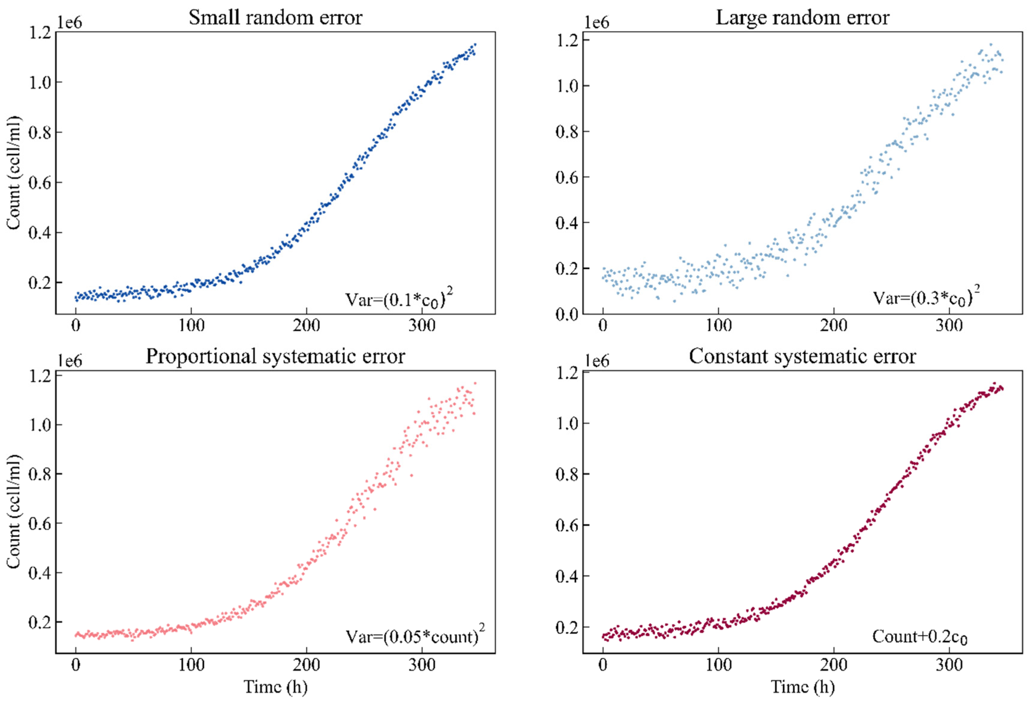
First, to compare different sampling designs, this study simulates four scenarios based on different kinds of experimental errors. Each scenario contains two hundred simulated experimental observation points. Scenario I: the observation data are normally distributed with a small random error, and the standard deviation is set to 0.1 times the nominal value of parameter c0. Scenario II: the observation data are normally distributed with a large random error, and the standard deviation is set to the value of 0.3 times the nominal value of parameter c0. Scenario III: the observation data are normally distributed with a proportional systematic error, and the standard deviation is 0.05 times the count. Scenario IV: for simplicity, the observation data are normally distributed with a constant systematic error, the same as in Scenario I. However, we add 0.2 times the nominal value of parameter c0 to the count. Figure 1 shows the simulated curves of the different error types. The blue color code is used for small random error, sky blue for large random error, red for proportional systematic error and magenta for constant systematic error.
Under each scenario, the total number of sampling points is set to 16 within each sampling design. We estimate the parameters of the logical growth model given by Equation (1) within different sampling designs under each scenario. Further, we compute designs on their prospective parameter calibration accuracy, and include the estimate’s MSE, covariance and bias as well as the FIM.
3. Results and Discussion
3.1. Model Fitting Results
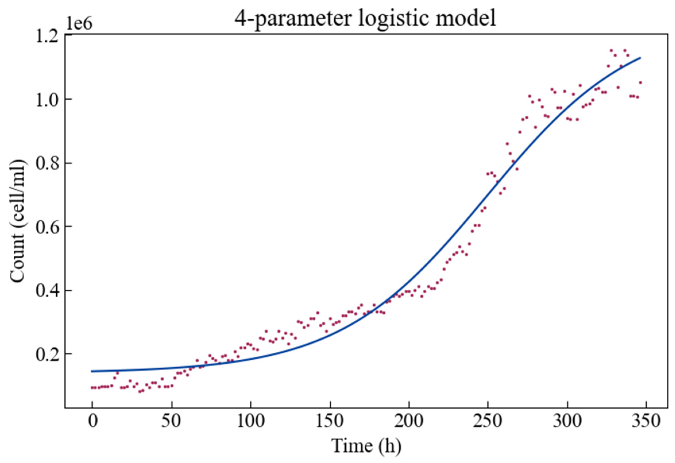
The experimental growth data together with the fitted four-parameter logistic growth model is shown in Figure 2. The growth curve is plotted as cell density (or cell/mL) versus time. Algae show a phase in which the specific growth rate starts at a minimum value, then accelerates to a maximum value for a certain period of time, and then gradually decreases. Therefore, there is a short adaptation phase, followed by an exponential phase of rapid population density growth then a stable phase of reaching a maximum population level.
Estimates for these parameters are given in Table 1, along with their respective statistics. The p-values indicate that all parameters can be estimated significantly. It is clear that the parameter d has the largest boundaries on the interval—i.e., it has the largest estimation error, and the parameter b has the smallest boundaries on the interval—the smallest estimation error. It is worth noting that when the curve trend is rising, the parameter b is a negative value. When the population density (, cell/mL) is close to c (cell/mL) or approaches d (cell/mL) then the slope of the logistic model (Equation (1)) approaches zero.
3.2. Optimal Sample Points and Confidence Interval
Table 2 shows the results of the optimal sampling points obtained by using a D-optimal design criterion. Since the growth model contains four model parameters, the number of corresponding optimal sampling points is also four. Assuming that the total experiment duration is 346 h, the sampling times of the four sampling points, in this case, are the 0th hour, the 142nd h, the 241st h, and the 346th h. Among these, the first sampling point is when the experiment starts, and the fourth sampling point is when the experiment ends, according to our assumption. It could also be shown that the third sampling point locates the exponential growth period correspondence.
According to the physical meaning of the model parameters, parameter b represents the position of the asymptotic line at the beginning of the curve. Combined with the time distribution of the sampling points obtained by D optimization, it can be inferred that the purpose of setting the first optimal sampling point at the beginning of the experiment is to determine the parameter c more accurately. Similarly, the last of the four optimal sampling points is at the end of the experiment; it measures the parameter d as closely as possible: that is, it determines the upper asymptote of the growth curve. Another noteworthy phenomenon is that the third optimal sampling point determines the maximum growth rate of the microalgae, which is related to Parameter b. Therefore, according to the exclusion method, the second optimal sampling point is used to determine the Parameter e.
As we assign all four parameters the same importance, all the four optimal sampling points have uniform weights—0.25. Thus, under the non-uniform sampling, we treat the four optimal sampling points equally and assign the same sampling times at or around each sampling point. The four optimal sampling points are also used as the center position in each sampling interval for the coupled sampling method proposed in this study. Therefore, of the 16 sampling points set in this study, four are arranged around each optimal sampling point. In addition, the sampling points corresponding to the first and last optimal sampling points need to be as close as possible to the start and end times of the experiment. This study assumes that sampling can only be performed once at the same time point—that sampling cannot be repeated. Moreover, all sampling times are taken as integers. For non-uniform sampling, we arrange the sample points in sequence at the beginning and end of the experiment as follows: 0 h, 1 h, 2 h, 3 h and 343 h, 344 h, 345 h, 346 h.
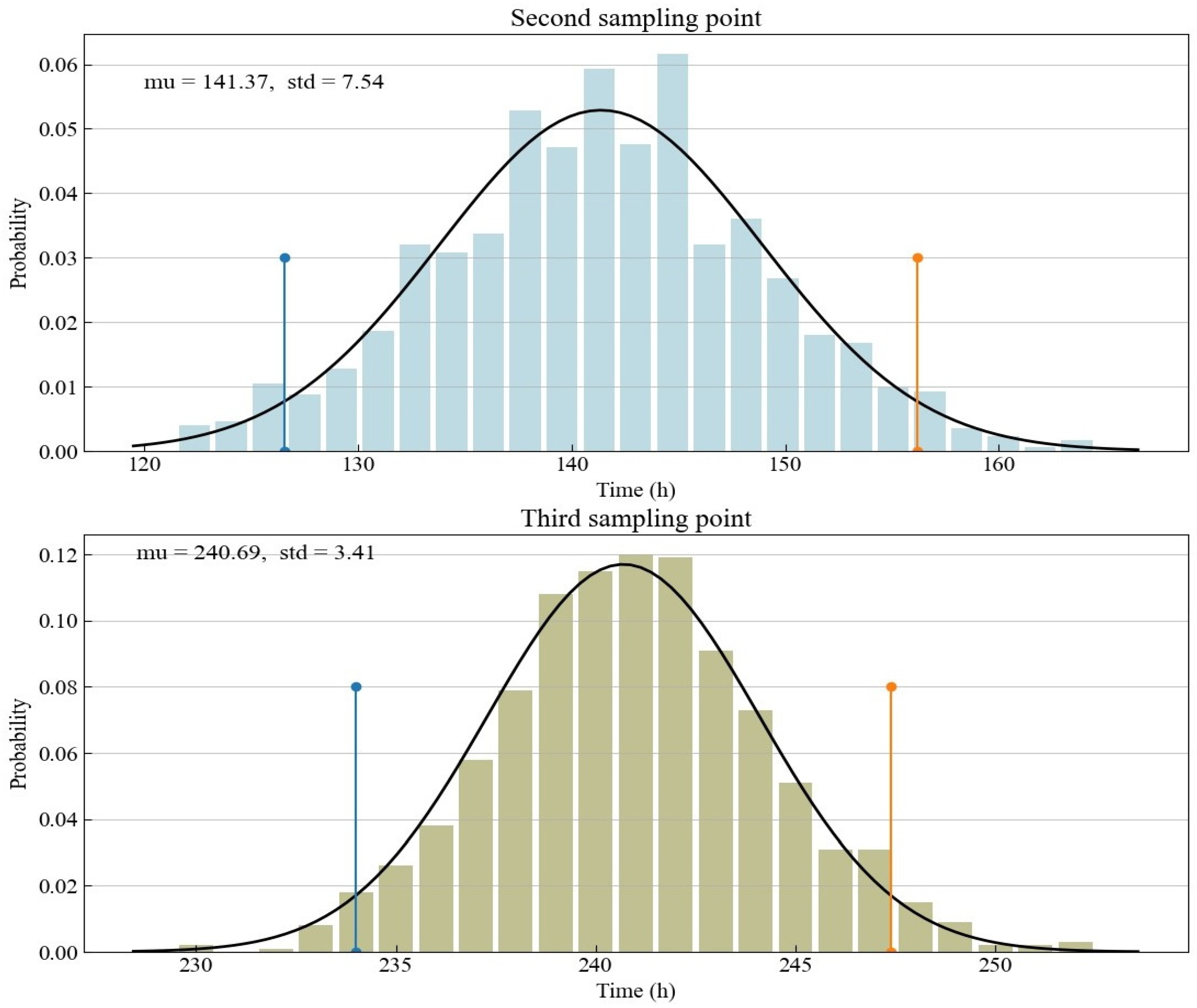
The focus of the experimental design is on the arrangement of sampling points related to the third and fourth optimal sampling points. The non-uniform sampling points are located next to the two optimal sampling points, while the distribution of sampling points in the coupled sampling method proposed in this study is slightly more dispersed. The optimal sampling point obtained from D optimization is conditioned on the prior knowledge from preliminary experiments or domain-specific knowledge. The specific prior knowledge here is mainly the nominal value of the model parameters. Since we use previous experiments to calibrate the nominal value in this study, there is a degree of uncertainty in our understanding of the nominal value. This study is based on the parameter fitting results of experimental data to determine the random parameter nominal values generated by Monte Carlo simulation. The distribution characteristics of the second and third optimal sampling points obtained according to the random nominal value are shown in Figure 3. Since the distribution of the nominal value of a parameter is a normal distribution, the time distribution of the optimal sampling point derived from the D optimization is also a normal distribution. Thus, we use a normal distribution to fit the time of the optimal sampling points. The upper and low bounds of the 95% confidence interval derived from the normal distribution are also shown in the yellow and blue lines in Figure 3 and Table 3. They directly determine the design space of the proposed coupled sampling method. Compared with the third optimal sampling point with the confidence interval ranging from about 234 to 247, the second optimal sampling point has a larger confidence interval, ranging from about 127 to 156.
In the ideal case, if we had a lot of data about the parameters, then a distribution of the parameters could be found. However, we do not have so many data to find the distribution of the parameters. We have chosen a normal distribution for the parameters taking into account previous knowledge [51]. However, the parameter distribution has a positive or negative shift, so the normal distribution can affect the accuracy of the results. The normal distribution is not ideal in many cases. Beta distribution is also an important distribution of the parameters. The beta distribution has a symmetrical and biased distribution, depending on the selected parameter values. Therefore, in the future, it is necessary to collect a large amount of data about the parameters to find the parameter distribution.
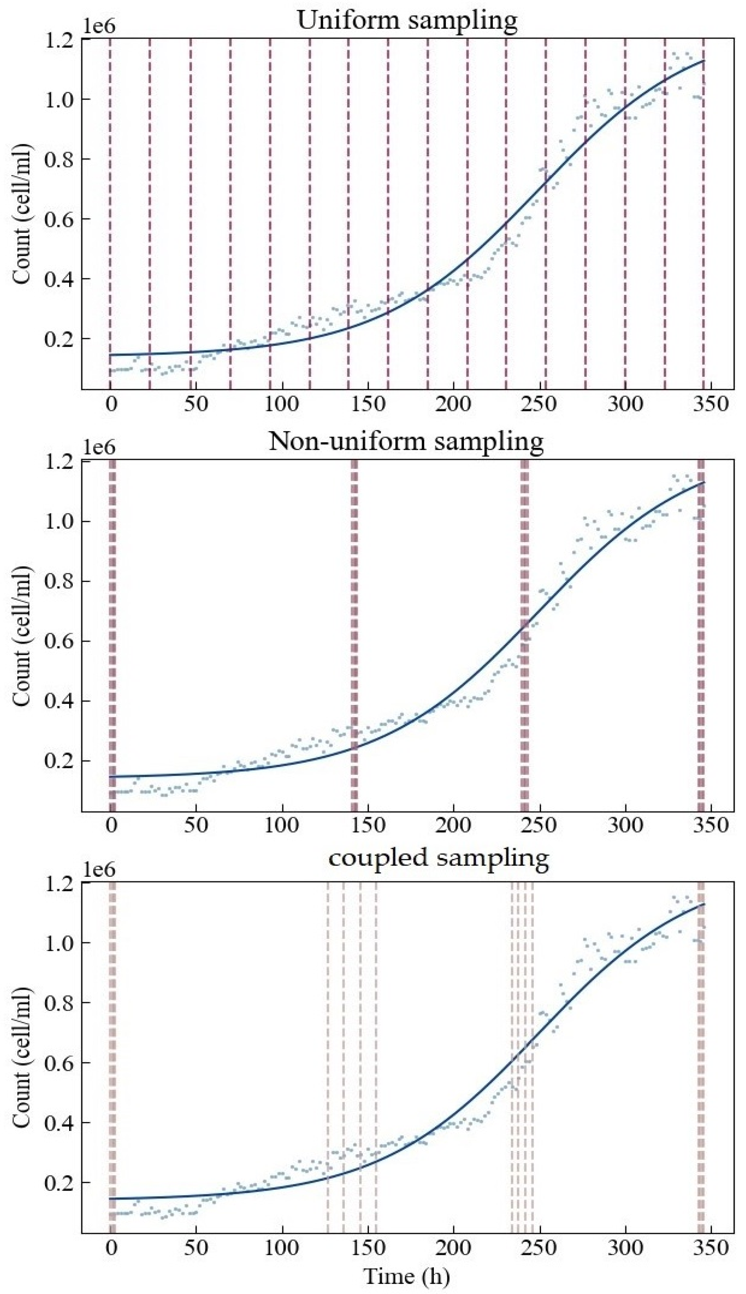
To conclude the process, we finalized the specific sampling implementation plan for different sampling methods (Figure 4). Under uniform sampling, 16 sampling points are evenly distributed in the design space. The non-uniform and coupled sampling points are roughly distributed around the four optimal sampling points obtained by D optimization. There are four points arranged around each optimal sampling point. The latter two methods tend to concentrate resources on the estimations of the four parameters. The main difference between these two methods is that the sampling range of coupled sampling is set wider. This is because at the start and the end, there is greater confidence that d and c can be estimated well, hence the narrow region, while at the central part, there is more uncertainty that d and c can be estimated well, hence the wider range.
3.3. Precision of the Parameter Estimates
Without conditions on the simulated experimental data, we first conducted a preliminary evaluation of the performance of the three sampling methods based on the nominal values of the parameters. The asymptotic approximation of the parameter accuracy metrics of each of the three sampling methods is shown in Table 4, Table 5 and Table 6. The accuracy metrics include FIM, covariance and bias, as well as MSE. FIM is the fundamental calculation basis for D optimization. The purpose of D optimization is to maximize the determinant of FIM by optimizing the locations and number of sampling points. Hence, we calculate and compare the D optimization as the determinant of the FIMs of the three sampling designs. After approximation, the determinants were calculated as 1.146 × 10⁻¹⁰, 1.672 × 10⁻¹⁰ and 1.618 × 10⁻¹⁰. It can be seen that the amount of information contained in the estimates of both non-uniform sampling and coupled sampling is relatively large, and the amount of information held in uniform sampling is the smallest. The covariance is approximated by the matrix inverse of the total FIM, which characterizes certain estimation intervals. The bias measures the expected difference between the estimate and the true parameter value. The MSE describes the second central moment of each parameter estimate around its true value.
It should be noted that the parameter accuracy metrics here are data-free methods. When the total number of samples is set the same, no sampling method can perform better in all the accuracy metrics. For example, uniform sampling has relative advantages in the bias and MSE of parameter b. However, the estimated performance of other parameters is not as good as in either non-uniform sampling or coupled sampling. The actual optimization goals and the trade-off among different accuracy metrics must be considered for any particular application in order to decode which sampling method is more reasonable in practice
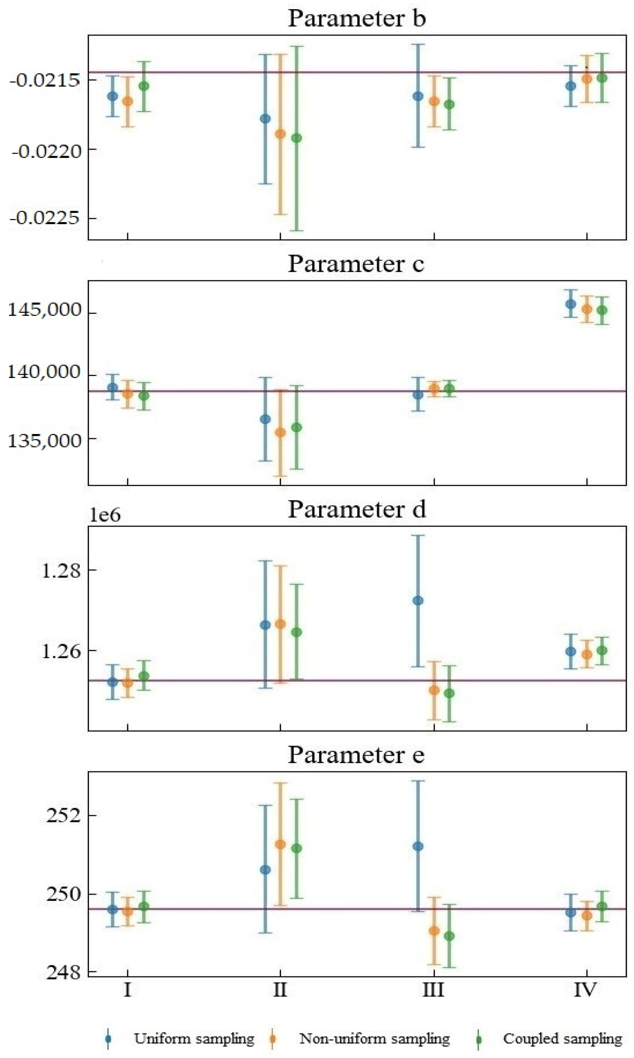
Figure 5 shows the fitting of the model parameters after substituting the simulated experimental data. A total of four sets of data (datasets from Scenarios I, II, III, IV) were generated in this study, and each set of data contains two hundred simulated experimental observation data points. The dot markers at the middle of the attached error bar represent the means of the estimated parameters. The upper and lower bounds of the attached error bars represent the 95% confidence intervals. The red horizontal lines indicate the nominal values used to simulate the dataset. Unlike the above-mentioned data-free analysis results, this analysis considers the experimental data of different types of experimental errors.
The combination of different observation errors and sampling methods will have complex and diverse effects on parameter estimation. Considering datasets from Scenarios I and IV, when the random error of the observation is small, the sizes of the confidence intervals corresponding to different sampling methods do not differ much. The difference is mainly reflected in the mean value of the parameter estimates. The confidence intervals corresponding to datasets for Scenarios II and III are relatively large, indicating that the observation error is crucial in determining parameter estimation uncertainty. The proportional systematic error in Scenario III will cause considerable parameter estimation result deviation between uniform sampling and the other two kinds of sampling. For one thing, it will cause the confidence interval of uniform sampling to be wider than those of either non-uniform or coupled sampling. The mean values of the estimated Parameters c, d, and e of uniform sampling and the mean values of the other two kinds of sampling are distributed on opposite sides of the nominal value. What is more, the mean values of the uniform sampling are farther away from the nominal values.
Our proposed coupled sampling method is more suitable for an observation dataset with small variance and observation errors. In Scenario I, coupled sampling is the only sampling design that can ensure that the nominal value of parameter b is in the 95% confident interval. In contrast, the other sampling methods may produce inaccurate or incorrect inferences for the model, Parameter b. When the observation error is significant, the proposed coupled sampling method can often provide more accurate parameter estimation for c and d than can non-uniform sampling, because the observation points of coupled sampling are more widely scattered—closer to the beginning and end of the experiment—than the observation points of non-uniform sampling: that is to say, closer to the best time to determine d and c.
Coupled sampling can perform slightly better than other sampling methods for the mean value of parameter estimation. When sampling needs to be repeated, uniform sampling will result in a waste of resources. At this time, certain prior information is helpful for preliminary estimation of model parameters. Furthermore, coupled sampling is very helpful for knowing when to measure the growth curve. D-optimal sampling relies on certain prior knowledge to find the optimal sampling point. However, the disadvantage of D-optimal sampling is that it places a strong emphasis on the most sensitive parameters. In addition, it may show increased correlation among the parameters, despite the decrease in the total confidence interval.
The coupled experimental design is based on D-optimal design, with uniform sampling in the confidence interval, which can solve the optimal number of problems and optimize resource utilization but there are some limitations. Firstly, the coupled experiment design ignored the situation of repeated sampling at a given time. Due to the limitations of the automatic plate reader which requires time to take a picture, it can only obtain one observation at any given time. There can be no multiple measurements or resampling at the same time in the strict sense. Secondly, in this study, the coupled experiment design did not consider the case where the weights of the optimal sampling points are not equal. Weighting is a critical factor affecting the sample size assigned to the sampling points. Assigning unequal weights can definitively affect the experiment design results. For example, we can assign larger weights at the central part and less weights at the start and end. Larger weights at the central part will have larger sample sizes. This can improve parameter estimation accuracy. This problem is very complex and may introduce a lot of work to solve. It is our limitation for this study, and we think we could study effects of different weights in the future. This will be a very good research topic.
4. Conclusions
Sampling design is critical to parameter estimation, and a suitable sampling schedule can improve the estimation accuracy while reducing labor and economic costs. Based on D optimization, the widely used non-uniform sampling relies on prior knowledge—more precisely, the nominal value of the parameter. Current sampling designs often fail to account for the uncertainty associated with the nominal value setting in the optimization, and will ultimately lead to poor parameter estimates. To handle this uncertainty problem, we have proposed a new sampling design that couples the idea of both uniform and non-uniform sampling. Based on D optimization, the sampling domain corresponding to each parameter is decided by the confidence interval obtained from the Monte Carlo simulation of the optimal sampling points, which is roughly derived from the concept of non-uniform sampling. We then suggest conducting uniform sampling in the above-mentioned sampling domain to further reduce the impact of uncertainty.
To demonstrate the performance of the proposed sampling method, we used the four-parameter logistic model as a mathematical model, and simulated the experimental observation data with different kinds of experiment errors. The three kinds of sampling methods—uniform sampling, non-uniform sampling based on D optimization, and our newly developed coupled method—were tested against a simulated dataset. When the experimental data have only a fixed number of random observation errors, the three sampling methods perform basically at the same level. However, when the simulated data present systematic errors proportional to the observed values, non-uniform sampling and coupled sampling have a practical advantage over uniform sampling in parameter estimates, showing a smaller confidence interval and being closer to the nominal value. When there is a fixed systematic observation error, the sampling method proposed in this study benefits from the characteristics of both concentration and dispersion, making it slightly better than other sampling methods for determining the mean value of parameter estimation.
For experiment designs in the study of microalgae growth, it is important to consider various sampling strategies such as the coupled method developed in this study. At the same time, the use of experimental instruments with higher observational accuracy and the standardization of experimental operating procedures will also be beneficial to the estimation of model parameters.
Author Contributions
Conceptualization, H.L. and E.Z.; methodology, H.L. and E.Z.; investigation, H.L. and E.Z.; data curation, H.L. and E.Z.; formal analysis, H.L. and E.Z.; writing—original draft preparation, H.L. and E.Z.; writing—review and editing, H.L. and E.Z.; resources, H.L. and E.Z.; project administration, H.L. and E.Z. All authors have read and agreed to the published version of the manuscript.
Funding
We thank the National Natural Science Foundation of China (52079007) for their financial support.
Institutional Review Board Statement
Not applicable.
Informed Consent Statement
Not applicable.
Data Availability Statement
Data are available on-demand from the corresponding author.
Acknowledgments
We would like to extend special thanks to the editor and the anonymous reviewers for their valuable comments in significantly improving this paper’s quality.
Conflicts of Interest
The authors declare no conflict of interest.
References
- Foster, R.A.; Zehr, J.P. Diversity, genomics, and distribution of phytoplankton-cyanobacterium single-cell symbiotic associations. Annu. Rev. Microbiol. 2019, 73, 435–456. [Google Scholar] [CrossRef] [PubMed]
- Ramaraj, R.; Tsai, D.D.W.; Chen, P.H. An exploration of the relationships between microalgae biomass growth and related environmental variables. J. Photochem. Photobiol. B 2014, 135, 44–47. [Google Scholar] [CrossRef]
- Wágner, D.S.; Valverde-Perez, B.; Sæbø, M.; de la Sotilla, M.B.; Van Wagenen, J.; Smets, B.F.; Plosz, B.G. Towards a consensus-based biokinetic model for green microalgae–The ASM-A. Water Res. 2016, 103, 485–499. [Google Scholar] [CrossRef] [Green Version]
- Swinnen, I.A.M.; Bernaerts, K.; Dens, E.J.J.; Geeraerd, A.H.; Van Impe, J.F. Predictive modelling of the microbial lag phase: A review. Int. J. Food Microbiol. 2004, 94, 137–159. [Google Scholar] [CrossRef]
- Perin, G.; Bernardi, A.; Bellan, A.; Bezzo, F.; Morosinotto, T. A mathematical model to guide genetic engineering of photosynthetic metabolism. Metab. Eng. 2017, 44, 337–347. [Google Scholar] [CrossRef]
- Chang, H.X.; Huang, Y.; Fu, Q.; Liao, Q.; Zhu, X. Kinetic characteristics and modeling of microalgae Chlorella vulgaris growth and CO2 biofixation considering the coupled effects of light intensity and dissolved inorganic carbon. Bioresour. Technol. 2016, 206, 231–238. [Google Scholar] [CrossRef]
- Mytilinaios, I.; Salih, M.; Schofield, H.K.; Lambert, R.J.W. Growth curve prediction from optical density data. Int. J. Food Microbiol. 2012, 154, 169–176. [Google Scholar] [CrossRef] [Green Version]
- Wagner, D.S.; Cazzaniga, C.; Steidl, M.; Dechesne, A.; Valverde-Perez, B.; Plosz, B.G. Optimal influent N-to-P ratio for stable microalgal cultivation in water treatment and nutrient recovery. Chemosphere 2021, 262, 127939. [Google Scholar] [CrossRef] [PubMed]
- Tjorve, K.M.C.; Tjorve, E. The use of Gompertz models in growth analyses, and new Gompertz-model approach: An addition to the Unified-Richards family. PLoS ONE. 2017, 12, e0178691. [Google Scholar] [CrossRef] [PubMed]
- Konopacki, M.; Augustyniak, A.; Grygorcewicz, B.; Dołęgowska, B.; Kordas, M.; Rakoczy, R. Single Mathematical Parameter for Evaluation of the Microorganisms’ Growth as the Objective Function in the Optimization by the DOE Techniques. Microorganisms 2020, 8, 1706. [Google Scholar] [CrossRef]
- Hall, B.G.; Acar, H.; Nandipati, A.; Barlow, M. Growth rates made easy. Mol. Biol. Evol. 2014, 31, 232–238. [Google Scholar] [CrossRef] [PubMed] [Green Version]
- Hossain, N.; Mahlia, T.M.I. Progress in physicochemical parameters of microalgae cultivation for biofuel production. Crit. Rev. Biotechnol. 2019, 39, 835–859. [Google Scholar] [CrossRef] [PubMed]
- Vilas, C.; Arias-Méndez, A.; García, M.R.; Alonso, A.A.; Balsa-Canto, E. Toward predictive food process models: A protocol for parameter estimation. Crit. Rev. Food Sci. 2018, 58, 436–449. [Google Scholar] [CrossRef]
- Wright, S.E.; Bailer, A.J. Optimal experimental design for a nonlinear response in environmental toxicology. Biometrics 2006, 62, 886–892. [Google Scholar] [CrossRef]
- Hagen, D.R.; White, J.K.; Tidor, B. Convergence in parameters and predictions using computational experimental design. Interface Focus. 2013, 3, 20130008. [Google Scholar] [CrossRef] [PubMed] [Green Version]
- Chandran, K.; Smets, B.F. Optimizing experimental design to estimate ammonia and nitrite oxidation biokinetic parameters from batch respirograms. Water Res. 2005, 39, 4969–4978. [Google Scholar] [CrossRef]
- Peñalver-Soto, J.L.; Garre, A.; Esnoz, A.; Fernández, P.S.; Egea, J.A. Guidelines for the design of (optimal) isothermal inactivation experiments. Food Res. Int. 2019, 126, 108714. [Google Scholar] [CrossRef]
- Vilmin, L.; Flipo, N.; Escoffier, N.; Groleau, A. Research, P. Estimation of the water quality of a large urbanized river as defined by the European WFD: What is the optimal sampling frequency? Environ. Sci. Pollut. R. 2018, 25, 23485–23501. [Google Scholar] [CrossRef] [Green Version]
- Kreutz, C.; Timmer, J. Systems biology: Experimental design. FEBS J. 2009, 276, 923–942. [Google Scholar] [CrossRef]
- Chen, Y.B.; Chen, J.X.; Chen, X.; Wang, M.; Wang, W. Uniform Sampling Table Method and its Applications II—Evaluating the Uniform Sampling by Experiment. J. AOAC Int. 2015, 98, 1455–1461. [Google Scholar] [CrossRef]
- Dai, Y.P.; Chen, X.L.; Yin, J.P.; Wang, G.D.; Wang, B.; Zhan, Y.H.; Nie, Y.Z.; Wu, K.C.; Liang, J.M. Investigation of the influence of sampling schemes on quantitative dynamic fluorescence imaging. Biomed. Opt. Express 2018, 9, 1859–1870. [Google Scholar] [CrossRef] [Green Version]
- Jaques, A.V.; Barraza, M.B.; Lacombe, J.C. The impact of variable measurement spacing in concentration profiles used in diffusion experiments. J. Phase Equilib. Diff. 2015, 36, 22–27. [Google Scholar] [CrossRef]
- Dragalin, V.; Fedorov, V.; Wu, Y.H. Adaptive designs for selecting drug combinations based on efficacy–toxicity response. J. Stat. Plan. Infer. 2008, 138, 352–373. [Google Scholar] [CrossRef]
- Holland-Letz, T.; Kopp-Schneider, A. Optimal experimental designs for dose–response studies with continuous endpoints. Arch. Toxicol. 2015, 89, 2059–2068. [Google Scholar] [CrossRef] [Green Version]
- Altmann-Dieses, A.E.; Schlöder, J.P.; Bock, H.G.; Richter, O. Optimal experimental design for parameter estimation in column outflow experiments. Water Resour. Res. 2002, 38, 4-1–4-11. [Google Scholar] [CrossRef]
- Smucker, B.; Krzywinski, M.; Altman, N. Optimal experimental design. Nat. Methods 2018, 15, 559–560. [Google Scholar] [CrossRef]
- Schenk, J.; Poeter, E.; Navidi, W. Demystifying Fisher information: What observation data reveal about our models. Groundwater 2018, 56, 547–556. [Google Scholar] [CrossRef]
- Muñoz-Tamayo, R.; Martinon, P.; Bougaran, G.; Mairet, F.; Bernard, O. Getting the most out of it: Optimal experiments for parameter estimation of microalgae growth models. J. Process. Control 2014, 24, 991–1001. [Google Scholar] [CrossRef] [Green Version]
- Li, G.; Majumdar, D. D-optimal designs for logistic models with three and four parameters. J. Stat. Plan. Infer. 2008, 138, 1950–1959. [Google Scholar] [CrossRef]
- Yao, K.Z.; Shaw, B.M.; Kou, B.; McAuley, K.B.; Bacon, D.W. Modeling ethylene/butene copolymerization with multi-site catalysts: Parameter estimability and experimental design. Polym. React. Eng. 2003, 11, 563–588. [Google Scholar] [CrossRef]
- Swintek, J.; Etterson, M.; Flynn, K.; Johnson, R. Optimized temporal sampling designs of the Weibull growth curve with extensions to the von Bertalanffy model. Environmetrics 2019, 30, e2552. [Google Scholar] [CrossRef]
- Sinkoe, A.; Hahn, J. Optimal Experimental Design for Parameter Estimation of an IL-6 Signaling Model. Processes 2017, 5, 49. [Google Scholar] [CrossRef]
- Props, R.; Rubbens, P.; Besmer, M.; Buysschaert, B.; Sigrist, J.; Weilenmann, H.; Waegeman, W.; Boon, N.; Hammes, F. Detection of microbial disturbances in a drinking water microbial community through continuous acquisition and advanced analysis of flow cytometry data. Water Res. 2018, 145, 73–82. [Google Scholar] [CrossRef]
- Li, H.; Lyu, P.J.; Sun, Y.C.; Wang, Y.; Liang, X.Y. A quantitative study of 3D-scanning frequency and Δd of tracking points on the tooth surface. Sci. Rep.-UK 2015, 5, 14350. [Google Scholar] [CrossRef] [Green Version]
- Coluccio, M.L.; Perozziello, G.; Malara, N.; Parrotta, E.; Zhang, P.; Gentile, F.; Limongi, T.; Raj, P.M.; Cuda, G.; Candeloro, P.; et al. Microfluidic platforms for cell cultures and investigations. Microelectron. Eng. 2019, 208, 14–28. [Google Scholar] [CrossRef]
- Teo, C.L.; Atta, M.; Bukhari, A.; Taisir, M.; Yusuf, A.M.; Idris, A. Enhancing growth and lipid production of marine microalgae for biodiesel production via the use of different LED wavelengths. Bioresource Technol. 2014, 162, 38–44. [Google Scholar] [CrossRef]
- Paakkunainen, M.; Reinikainen, S.P.; Minkkinen, P. Estimation of the variance of sampling of process analytical and environmental emissions measurements. Chemometr. Intell. Lab. 2007, 88, 26–34. [Google Scholar] [CrossRef]
- Tamburic, B.; Evenhuis, C.R.; Crosswell, J.R.; Ralpha, P.J. An empirical process model to predict microalgal carbon fixation rates in photobioreactors. Algal Res. 2018, 31, 334–346. [Google Scholar] [CrossRef]
- Bernaerts, K.; Gysemans, K.P.m.; Nhan Minh, T.; Van Impe, J.F. Optimal experiment design for cardinal values estimation: Guidelines for data collection. Int. J. Food Microbiol. 2005, 100, 153–165. [Google Scholar] [CrossRef]
- Liu, M.D.; Wu, T.; Zhao, X.Y.; Zan, F.Y.; Yang, G.; Miao, Y.P. Cyanobacteria blooms potentially enhance volatile organic compound (VOC) emissions from a eutrophic lake: Field and experimental evidence. Environ. Res. 2021, 202, 111664. [Google Scholar] [CrossRef] [PubMed]
- Chèvre, N.; Brazzale, A.R. Cost-effective experimental design to support modeling of concentration–response functions. Chemosphere 2008, 72, 803–810. [Google Scholar] [CrossRef]
- Hu, Y.; Meng, F.L.; Hu, Y.Y.; Habibul, N.; Sheng, G.P. Concentration-and nutrient-dependent cellular responses of microalgae Chlorella pyrenoidosa to perfluorooctanoic acid. Water Res. 2020, 185, 116248. [Google Scholar] [CrossRef]
- Kamimura, Y.; Tanaka, H.; Kobayashi, Y.; Shikanai, T.; Nishimura, Y. Chloroplast nucleoids as a transformable network revealed by live imaging with a microfluidic device. Commun. Biol. 2018, 1, 47. [Google Scholar] [CrossRef]
- Lai, H.T.; Hou, J.H.; Su, C.I.; Chen, C.L. Effects of chloramphenicol, florfenicol, and thiamphenicol on growth of algae Chlorella pyrenoidosa, Isochrysis galbana, and Tetraselmis chui. Ecotox. Environ. Safe 2009, 72, 329–334. [Google Scholar] [CrossRef]
- Tsoularis, A.; Wallace, J. Analysis of logistic growth models. Math. Biosci. 2002, 179, 21–55. [Google Scholar] [CrossRef] [Green Version]
- Cramer, J.S. The early origins of the logit model. Stud. Hist. Phi. Part C 2004, 35, 613–626. [Google Scholar] [CrossRef]
- Dalgaard, P.; Koutsoumanis, K. Comparison of maximum specific growth rates and lag times estimated from absorbance and viable count data by different mathematical models. J. Microbiol. Meth. 2001, 43, 183–196. [Google Scholar] [CrossRef]
- Ritz, C.; Streibig, J.C. Bioassay analysis using R. J. Stat. Softw. 2005, 12, 1–22. [Google Scholar] [CrossRef] [Green Version]
- Braniff, N. Optimal Experimental Design Applied to Models of Microbial Gene Regulation. Ph.D. Thesis, University of Waterloo, Waterloo, ON, Canada, 2020. [Google Scholar]
- Bonate, P.L. A brief introduction to Monte Carlo simulation. Clin. Pharmacokinet. 2001, 40, 15–22. [Google Scholar] [CrossRef]
- Grijspeerdt, K.; Vanrolleghem, P. Estimating the parameters of the Baranyi model for bacterial growth. Int. J. Food Microbiol. 1999, 16, 593–605. [Google Scholar] [CrossRef]
Figure 1.
Simulated curves of the different error types. Blue: small random error (σ = 0.1c0); sky blue: large random error (σ = 0.3c0); red: proportional systematic error (σ = 0.05count); magenta: constant systematic error (σ = count + 0.2c0).
Figure 1.
Simulated curves of the different error types. Blue: small random error (σ = 0.1c0); sky blue: large random error (σ = 0.3c0); red: proportional systematic error (σ = 0.05count); magenta: constant systematic error (σ = count + 0.2c0).

Figure 2.
The four-parameter logistic growth model fitted to the Scenedesmus obliquus growth curve.

Figure 3.
Histograms for the optimal Sample Points 2 and 3 as determined by Monte Carlo simulation.

Figure 4.
Specific sampling implementation plans for three different sampling methods.

Figure 5.
Fitting of the model parameters after substituting the simulated experimental data.


Table 1.
Parameter estimates.
| Parameter | Estimate | Std. Error | t-Value | p-Value |
|---|---|---|---|---|
| b | −2.145 × 10⁻² | 1.649 × 10⁻³ | −13.008 | <0.001 *** |
| c | 1.387 × 10⁵ | 1.179 × 10⁴ | 11.772 | <0.001 *** |
| d | 1.253 × 10⁶ | 4.326 × 10⁴ | 28.953 | <0.001 *** |
| e | 2.496 × 10² | 3.992 | 62.532 | <0.001 *** |
*** Significance at the p < 0.001 levels, respectively.
Table 2.
Results of the optimal sampling points obtained using a D-optimal design criterion.
| Sample Point | Time | Weights |
|---|---|---|
| 0 | 0 | 0.25 |
| 1 | 142 | 0.25 |
| 2 | 241 | 0.25 |
| 3 | 346 | 0.25 |
Table 3.
The 95% confidence intervals of Sample Points 2 and 3.
| Sample Point | 95% Confidence Intervals | |
|---|---|---|
| Lower | Upper | |
| 2 | 127 | 156 |
| 3 | 234 | 247 |
Table 4.
Asymptotic approximations of the parameter accuracy metrics of uniform sampling.
| Parameter | FIM | Covariance | Bias | MSE | ||||||
|---|---|---|---|---|---|---|---|---|---|---|
| b | c | d | e | b | c | d | e | |||
| b | 5.19 × 10⁶ | 0.2659 | 0.1147 | 1.39 × 10² | 1.15 × 10⁶ | 5.8530 | 30.9349 | 0.0028 | 0.0001 | 1.15 × 10⁻⁶ |
| c | 0.2659 | 4.83 × 10⁻⁸ | 9.55 × 10⁻⁹ | 0.0001 | 5.8530 | 6.46 × 10⁷ | 1.2 × 10⁸ | 6.88 × 10³ | 1.25 × 10³ | 6.55 × 10⁷ |
| d | 0.1147 | 9.55 × 10⁻⁹ | 1.58 × 10⁻⁸ | 0.0001 | 30.9350 | 1.2 × 10⁸ | 1.04 × 10⁹ | 9.86 × 10⁴ | 6.67 × 10³ | 1.08 × 10⁹ |
| e | 1.39 × 10² | 0.0001 | 0.0001 | 0.9793 | 0.0028 | 6.88 × 10³ | 9.8578 × 10⁴ | 10.5297 | 0.5960 | 10.7796 |
Table 5.
Asymptotic approximations of the parameter accuracy metrics of non-uniform sampling.
| Parameter | FIM | Covariance | Bias | MSE | ||||||
|---|---|---|---|---|---|---|---|---|---|---|
| b | c | d | e | b | c | d | e | |||
| b | 4.55 × 10⁶ | 0.2153 | 0.1569 | 1.63 × 10² | 1.44 × 10⁻⁶ | 6.1712 | 25.452 | 0.0025 | 3.40 × 10⁻⁷ | 1.40 × 10⁻⁶ |
| c | 0.2153 | 4.41 × 10⁻⁸ | 9.04 × 10⁻⁹ | 0.0001 | 6.1712 | 5.66 × 10⁷ | 1 × 10⁸ | 6.09 × 10³ | 6.22 × 10² | 5.64 × 10⁷ |
| d | 0.1569 | 9.04 × 10⁻⁹ | 2.09 × 10⁻⁸ | 0.0001 | 25.452 | 1 × 10⁸ | 5.68 × 10⁸ | 5.80 × 10⁴ | 1.82 × 10³ | 5.65 × 10⁸ |
| e | 1.63 × 10² | 0.0001 | 0.0001 | 0.9278 | 0.0025 | 6.09 × 10³ | 5.80 × 10⁴ | 7.4048 | 0.2505 | 7.3935 |
Table 6.
Asymptotic approximations of the parameter accuracy metrics of coupled sampling.
| Parameter | FIM | Covariance | Bias | MSE | ||||||
|---|---|---|---|---|---|---|---|---|---|---|
| b | c | d | e | b | c | d | e | |||
| b | 4.56 × 10⁶ | 0.2173 | 0.1544 | 2.02 × 10² | 1.82 × 10⁻⁶ | 7.9475 | 30.1286 | 0.0028 | 5.01 × 10⁻⁵ | 1.81 × 10⁻⁶ |
| c | 0.2173 | 4.44 × 10⁻⁸ | 8.99 × 10⁻⁹ | 0.0001 | 7.9475 | 7.47 × 10⁷ | 1.10 × 10⁸ | 4.73 × 10³ | 84.2448 | 7.39 × 10⁷ |
| d | 0.1544 | 8.99 × 10⁻⁹ | 2.08 × 10⁻⁸ | 0.0001 | 30.1286 | 1.10 × 10⁸ | 6.30 × 10⁸ | 6.36 × 10⁴ | 4.31 × 10³ | 6.42 × 10⁸ |
| e | 2.02 × 10² | 0.0001 | 0.0001 | 0.9209 | 0.0028 | 4.73 × 10³ | 6.36 × 10⁴ | 8.4634 | 0.7047 | 8.8753 |
Publisher’s Note: MDPI stays neutral with regard to jurisdictional claims in published maps and institutional affiliations. |
© 2021 by the authors. Licensee MDPI, Basel, Switzerland. This article is an open access article distributed under the terms and conditions of the Creative Commons Attribution (CC BY) license (https://creativecommons.org/licenses/by/4.0/).
Share and Cite
MDPI and ACS Style
Li, H.; Zhang, E. A Coupled Sampling Design for Parameter Estimation in Microalgae Growth Experiment: Maximizing the Benefits of Uniform and Non-Uniform Sampling. Water 2021, 13, 2996. https://doi.org/10.3390/w13212996
AMA Style
Li H, Zhang E. A Coupled Sampling Design for Parameter Estimation in Microalgae Growth Experiment: Maximizing the Benefits of Uniform and Non-Uniform Sampling. Water. 2021; 13(21):2996. https://doi.org/10.3390/w13212996
Chicago/Turabian StyleLi, Hao, and Enze Zhang. 2021. "A Coupled Sampling Design for Parameter Estimation in Microalgae Growth Experiment: Maximizing the Benefits of Uniform and Non-Uniform Sampling" Water 13, no. 21: 2996. https://doi.org/10.3390/w13212996
Note that from the first issue of 2016, this journal uses article numbers instead of page numbers. See further details here.