
Modelling Bathing Water Quality Using Official Monitoring Data
by
 and
and
Daniela Džal
1, 
Ivana Nižetić Kosović
2,
Toni Mastelić
2,
Damir Ivanković
3,
Tatjana Puljak
4 and
Slaven Jozić
3,* 1
Faculty of Science, Ruđera Boškovića 33, 21000 Split, Croatia
2
Ericsson Nikola Tesla, Poljička Cesta 39, 21000 Split, Croatia
3
Institute of Oceanography and Fisheries, Šetalište I. Meštrovića 63, 21000 Split, Croatia
4
Teaching Institute of Public Health of Split-Dalmatia County, Vukovarska 46, 21000 Split, Croatia
*
Author to whom correspondence should be addressed.
Water 2021, 13(21), 3005; https://doi.org/10.3390/w13213005
Submission received: 27 August 2021
/
Revised: 20 October 2021
/
Accepted: 22 October 2021
/
Published: 26 October 2021
(This article belongs to the Special Issue Healthy Recreational Waters: Sanitation and Safety Issues)
Abstract
:Predictive models of bathing water quality are a useful support to traditional monitoring and provide timely and adequate information for the protection of public health. When developing models, it is critical to select an appropriate model type and appropriate metrics to reduce errors so that the predicted outcome is reliable. It is usually necessary to conduct intensive sampling to collect a sufficient amount of data. This paper presents the process of developing a predictive model in Kaštela Bay (Adriatic Sea) using only data from regular (official) bathing water quality monitoring collected during five bathing seasons. The predictive modelling process, which included data preprocessing, model training, and model tuning, showed no silver bullet model and selected two model types that met the specified requirements: a neural network (ANN) for Escherichia coli and a random forest (RF) for intestinal enterococci. The different model types are probably the result of the different persistence of two indicator bacteria to the effects of marine environmental factors and consequently the different die-off rates. By combining these two models, the bathing water samples were classified with acceptable performances, an informedness of 71.7%, an F-score of 47.1%, and an overall accuracy of 80.6%.
1. Introduction
Bathing water quality is crucial to prevent the health risks associated with bathing in coastal and inland bathing waters. According to the Bathing Water Directive 2006/7/EC (BWD), the main document regulating the management and quality of bathing waters in the European Union (EU), its main objective is to protect human health and to preserve, protect, and improve the quality of the environment. As bathing water quality has been recognized as one of the most important reasons for tourists’ choice of destination [1,2], it is a crucial factor for island and coastal communities that depend on coastal tourism [3]. The Bathing Water Directive sets out the guidelines on monitoring, quality assessment, classification, and quality status of bathing waters and on information to the public. Bathing water assessment is based on the levels of two faecal indicator bacteria (FIB), Escherichia coli and intestinal enterococci. According to the BWD [4], the final assessment is based on bathing water quality data sets compiled for this and the three previous bathing seasons. The bathing water quality datasets used for the final assessment should always include at least 16 samples (based on an annual number of four samples) or 12 samples in the case of a bathing water located in a region with specific geographical constraints. The number of data during the bathing season depends on the length of the bathing season, which varies widely across EU Member States, ranging from two months in Sweden to six months in Cyprus [5]. This could theoretically lead to no sampling during some months in some Member States. Since most water quality exceedances are single-day events, even at the most frequently contaminated sites, there is a low chance (5%) of being detected at such low sampling frequency [6]. That leads to significant, 15–20% misclassification of bathing water sites [7]. Therefore, estimating compliance on the basis of such a small number of bathing water samples is unlikely to fulfill the main purpose of the BWD, which is to protect public health, as too many poor quality beaches could be classified in the better category [8]. Although the number of samples per bathing season is significantly higher than four in all Member States, WHO recommends a further increase to 20 samples per season [9]. This recommendation could lead to an additional financial burden and technical difficulties for many Member States. Furthermore, it is questionable whether it is justified to increase the number of samples at sites classified as ’excellent’ over a longer period of time.
To bridge the gap between the high cost of classical monitoring and the need for a high level of human health protection, additional tools could be used. One of the most popular is the development and application of water quality prediction models. It is recognised that predictive models can significantly enhance existing and provide novel preventive measures to protect human health. This especially refers to timely information on the quality of bathing water, unlike the current procedure based on the information on indicator bacteria counts in water samples that takes at least 24 h. The role of bathing water quality predicting is also recognized by World Health Organization (WHO) [9], who suggests that the bathing water classification may be upgraded by water quality prediction ’where recreational water is subject to occasional and predictable deterioration (such as after rainfall) and where users can effectively be discouraged from entering the water during such periods’ [7]. However, prediction of bathing water quality is hardly straightforward as the existing predictive models are not directly applicable to the described monitoring setup.
The overview of methods and results of predictive models for bathing water quality is given in [10]. As it can be concluded from the review, the most common model used is multiple linear regression (MLR) (especially considering literature older than 10 years) which assumes a linear relationship among parameters. Since the drivers of FIB concentration in bathing waters are more complex than can be characterized by a linear relationship, this model usually yields to variable (non-stable) results, deeply depending on the underlying data. In the last 10–15 years, other predictive models have been exploited, such as classification trees (CT), random forest (RF), neural network (ANN), etc. In their paper [11], the authors compare several models for E. coli prediction (MLR, ANN, CT, etc.) on daily measurements from Santa Monica beach in Los Angeles. The authors in [12] compare MLR and CT for E. coli prediction before and after the implementation of the Harbour Area Treatment Scheme on weekly measurements from three beaches in Hong Kong. The study on 20 Chicago beaches conducted in [13] exploits RF for prediction of E. coli.
The results of the above studies show high specificity and low sensitivity, which means that the model in most cases correctly predicts situations in which the bacteria level is low, but prediction of bacteria exceedance is in most cases poor. Moreover, each of the studies, naturally, is considering specificities of the sites investigated, resulting with the model, which is adapted to certain regions and parameters and in most cases cannot be directly applied to other sites.
In predictive modeling, it is crucial to choose the appropriate type of model (regression or classification) and appropriate metrics (accuracy, sensitivity, specificity, etc.) to minimize the errors [14,15]. In scenarios with imbalanced data, with a high proportion of data with a low level of indicator bacteria, reporting only accuracy yields the misleading conclusions, since accuracy in those cases can be high, while prediction of the bacteria exceedance can be poor [16,17]. In [18], the authors compare several models and metrics, stressing that choosing the best model highly depends on what we want to model. For example, the best model in their case is the Bayesian network which yields poor overall accuracy but high accuracy in the prediction of “red days” (days in which bacteria highly exceeds the threshold). The process of building the prediction model is nicely described in [19], although they apply it on estimating water quality index (WQI) not predicting E. coli.
The main objective of this paper is to assess whether a good and reliable predictive model for coastal bathing water quality can be built using only regular (official) monitoring data, or whether intensive sampling programs with more data on a spatial and temporal basis are needed.
2. Materials and Methods
2.1. Study Area
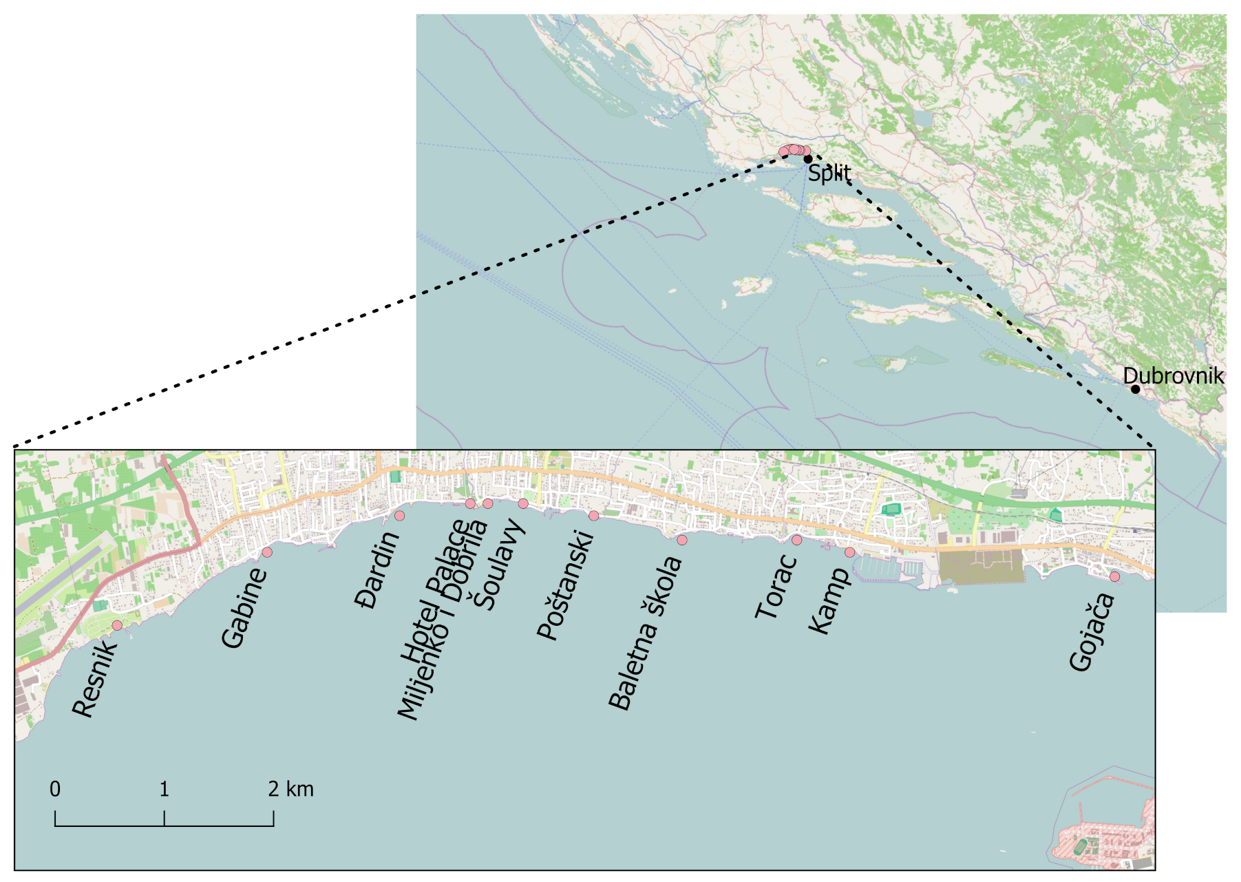
Kaštela Bay is 15 km long and 6 km wide, making it the largest bay in the central part of the coast of Croatian Adriatic (Figure 1). The bay is connected to the adjacent channel by a 1.8 km wide inlet. The average water renewal time (time period required to displace the entire volume of water in the bay) is about one month [20]. Due to heavy eutrophication and pollution caused by intensive industrialization (meat, cement, and chemical industries) and uncontrolled urbanization followed by uncontrolled discharge of wastewater from households, the bay was a hotspot and the most polluted area on the east coast of the Adriatic in the 1980s. With the construction of sewage systems for the surrounding cities and the closure of several industrial plants between 1990 and 2009, pollution in the bay has decreased significantly, especially in the eastern part of the bay [21]. As the sewage system in the most populated part of the bay (the town of Kaštela) has not yet been completed, this part is still under moderate pressure from faecal waters entering the bathing waters through many small uncontrolled sewage discharges near the coast. With many households connected to old leaky septic tanks, streams and groundwater are an additional source of contamination, especially after periods of rain. This is reflected in the quality of bathing waters in this area. In the final assessment in 2019, 4 out of 11 bathing sites in this area were assessed as poor and only four sites as excellent. This represents (4 out of 12) of all Croatian bathing sites assessed as poor in the 2019 final assessment (http://baltazar.izor.hr/plazepub/kakvoca_detalji10) (accessed on 10 March 2021). Based on these findings and the fact that this area is susceptible to unexpected and short-term pollution leading to water quality exceedances and thus higher health risks for bathers, it is clear that official monitoring could be supported by additional protection tools such as water quality prediction models.
Although not required by BWD, Regulation on Sea Bathing Water Quality [22] defines the standards and FIB limits for assessing bathing water quality after each sampling (Table 1). Bathing water is classified into four quality categories based on the concentration of indicator bacteria in samples taken at the predefined monitoring point. This is important because it provides a basis for the assessment of water quality after each sampling.
2.2. Dataset
Data are from the official monitoring program for coastal bathing waters conducted by Teaching Institute of Public Health of Split-Dalmatia County at 11 bathing sites in Kaštela Bay (Figure 1) during the 2015–2019 bathing seasons (n = 612 samples). The data are freely available to all institutions involved in the official monitoring of coastal waters in the Republic of Croatia, including Institute of Oceanography and Fisheries. Sampling for official monitoring was carried out fortnightly in the morning from the end of May to the end of September. The following features are collected during regular bathing water quality monitoring by Teaching Institute of Public Health of Split-Dalmatia County. For each sample, the timestamp and the location where the sample was taken are recorded. The salinity and temperature of the seawater are measured with a handheld probe directly at the time of sampling. Wind, precipitation, and weather description are estimated during sampling. E. coli and intestinal enterococci are determined by the membrane filtration method, temperature modified ISO 9308-1:2014 [23] for E. coli, and ISO 7899-2:2000 [24] for intestinal enterococci, respectively. Maximal and minimal tide levels are measured by a station at the Institute of Oceanography and Fisheries. Sewage outlets visible to the naked eye are mapped and the distance from the sampling point to the outlet is calculated.
Air temperature, humidity, pressure, pressure tendency, sea level pressure, wind speed, wind direction, cloud coverage, and precipitation in the last 24 h are collected from the Croatian Meteorological and Hydrological Service (https://meteo.hr/) (accessed on 17 March 2020). The values are approximated at the moment of sampling and day before, i.e., 24 h earlier using spatio-temporal interpolation.
Downward thermal infrared radiative flux, all sky insolation incident on a horizontal surface, top-of-atmosphere insolation, and insolation clearness index are acquired from the POWER Project, NASA (https://power.larc.nasa.gov/) as a daily (accessed on 19 March 2020) average all in the same position (center of the Kaštela bay). The number of tourist overnights for the entire area of the town of Kastela, as an indicator of the load on the area and consequently of the discharge of faecal waters, for the year 2016, come from the tourist board of Kaštela (https://www.kastela-info.hr/) (accessed on 2 April 2020). The number of tourists for other years are replicated data from the year 2016.
Average E. coli and intestinal enterococci levels in the past bathing season at the same bathing site and in the last sample on the same bathing site are added for both observed faecal indicators. Quality classes (based on only E. coli, only intestinal enterococci and combination of both bacteria) are calculated from the level of E. coli and intestinal enterococci according to the Marine Bathing Water Quality Regulation [22]. An overview of aforementioned features with their names used in modelling, description, and units is given in Table 2.
2.3. Predictive Modelling Process
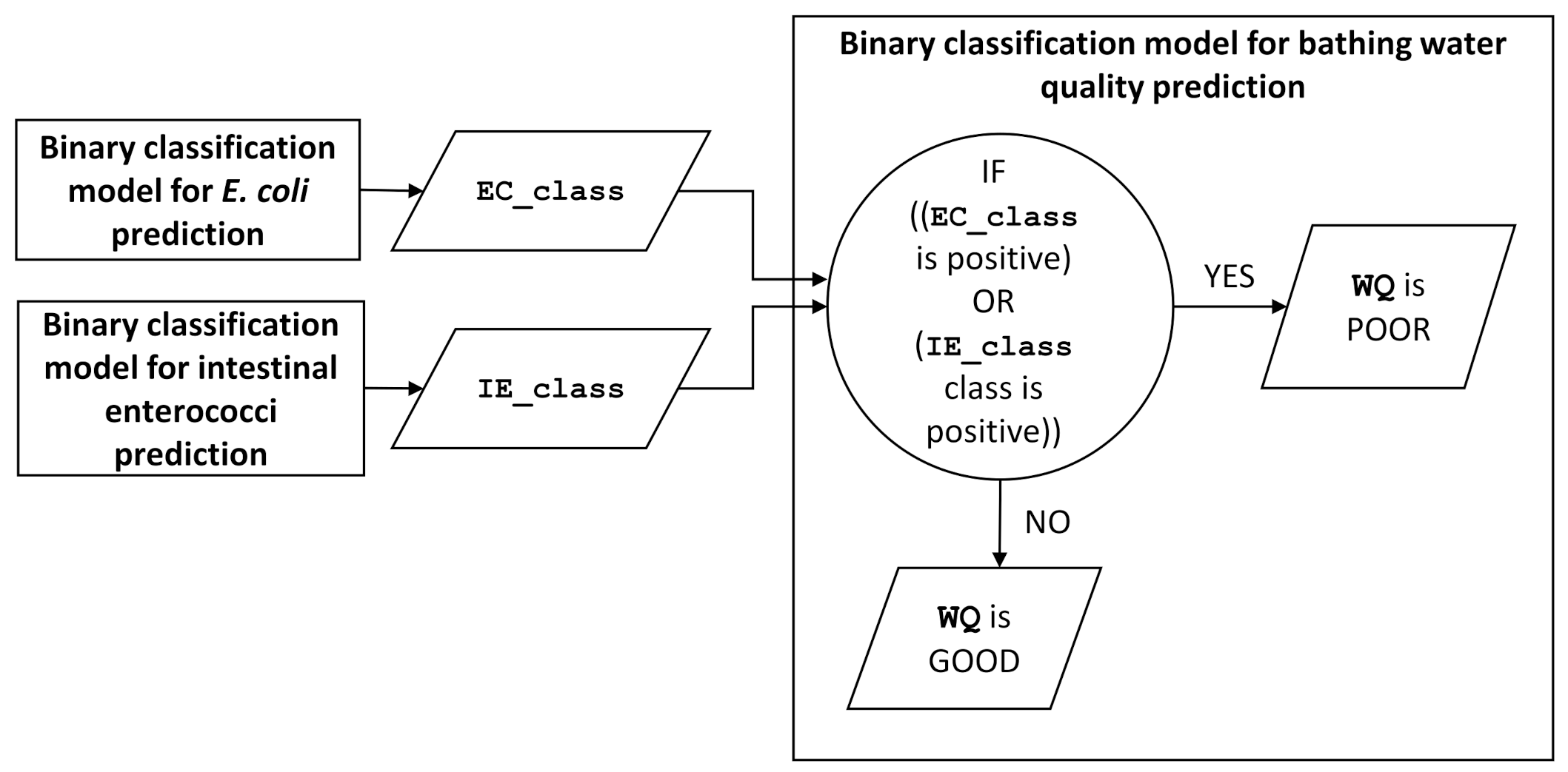
The dependent variable we want to model is the class of FIB exceedance—water quality (WQ). In this context, FIB exceedance is defined as poor water quality (>200 CFU/100 mL for intestinal enterococci and/or >300 CFU/100 mL for E. coli) as defined in Table 1. In the classification model, exceeding the selected FIB value is labeled as a positive class and the other samples as negative; therefore, a binary classification is chosen. According to BWD and Regulation on Sea Bathing Water Quality, two faecal bacteria are indicators for measuring bathing water quality. Two separate models are built for each bacteria (one with the dependent variable EC_class and another with IE_class). The results of the models are combined in the bathing water quality prediction model (WQ, illustrated in Figure 2): If the number of any of the FIB exceeds the sufficient bathing water quality, the quality is poor. The E. coli and intestinal enterococci levels, sample location and timestamp (loc, t, EC, and IE) are excluded from the modelling. Other features are considered as independent variables (Table 2).
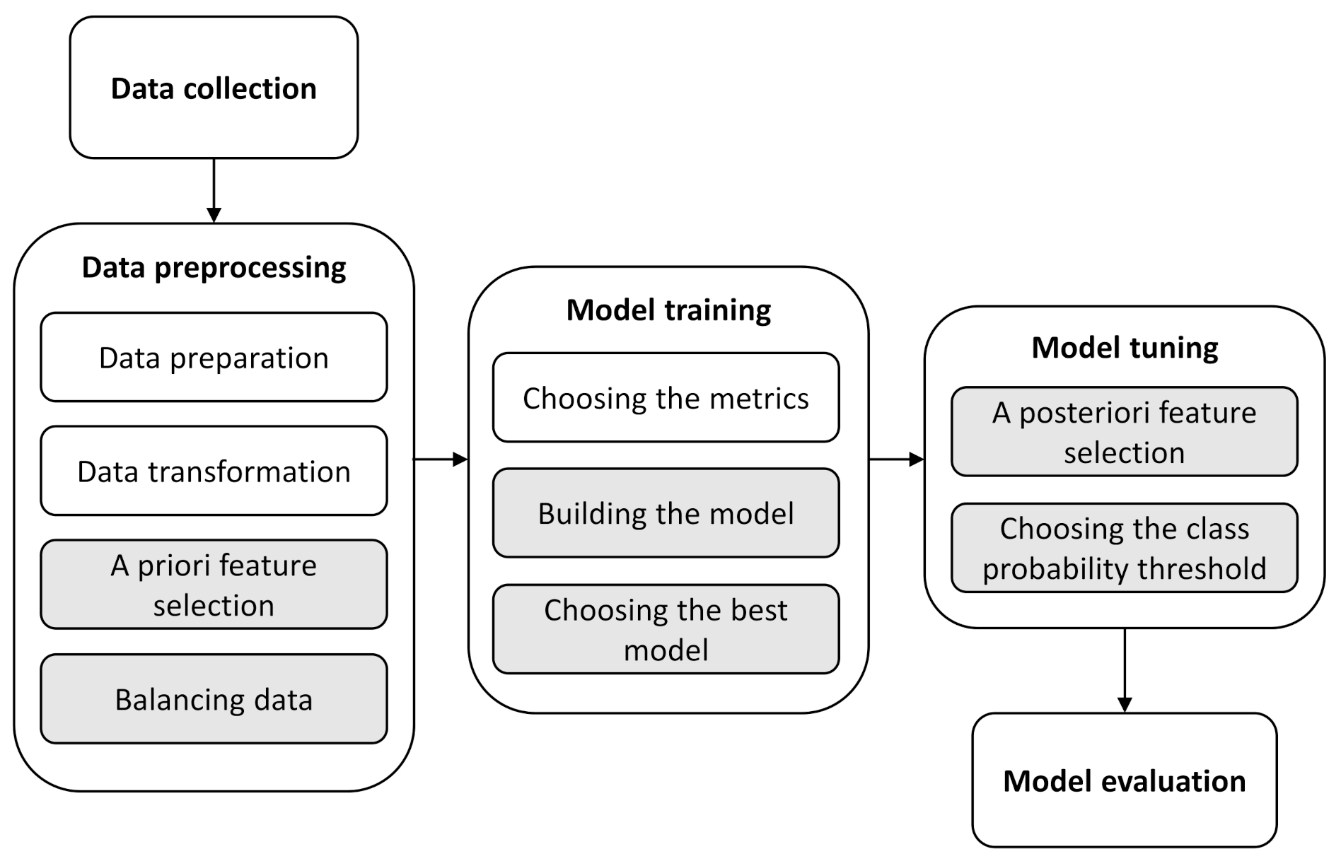
The process of predictive modelling for bathing water quality prediction is shown in Figure 3. The process follows the best practises of predictive modelling described in [25]. The process consists of five groups of steps: Data collection, Data preprocessing (containing four steps), Model training (containing three steps), Model tuning (containing two steps), and Model evaluation. The steps highlighted in white are performed for the dataset independently of the indicator bacteria we are modelling, and the steps highlighted in grey are performed separately for each indicator bacteria.
2.3.1. Data Preprocessing
The collected dataset was split into a training and holdout set. The holdout set was comprised of the data from the most recent sampling period to ensure the independence of these two datasets. All features in the training set are centered and scaled to have a mean of 0 and a standard deviation of 1 in the Data transformation step. Holdout data were fit to the same scale.
The next two steps are performed separately for each indicator bacteria: A priori feature selection and Balancing data. The first is required to reduce the number of independent parameters and is performed by calculating the correlation of the bacteria with other parameters and eliminating parameters that are weakly correlated to bacteria level. The second is required because the data are very imbalanced (with an extremely high ratio of negative to positive results). There are numerous algorithms to deal with class imbalance, and their performance also depends on the datasets [16]. In the context of bathing water quality, we had to combine several methods to deal with an imbalanced dataset due to the very low proportion of positive class samples. In this step, random under-sampling was chosen because it avoids the bias of synthetic data generation for extremely small minority classes, as in our case, and has better overall performance than over-sampling [26]. Random under-sampling randomly discards negative samples to achieve a more favorable positive/negative ratio. In the next steps, some other mechanisms are used to deal with class imbalance.
2.3.2. Model Training
The results of the modelling are presented in the form of a confusion matrix (Table 3), where true positive (TP) refers to the number of positive samples correctly classified, true negative (TN) refers to the number of negative samples correctly classified, false positive (FP) refers to the number of negative samples incorrectly classified as positive, and false negative (FN) refers to the number of positive samples incorrectly classified as negative.
There are several metrics used to evaluate classifier performance [25].
The most common metric is Accuracy, which expresses the proportion of correct results among all cases examined, given by the formula:
Accuracy, however, is not sufficient to describe how well the model works and may lead to incorrect conclusions, especially in the case of classification problems and imbalanced datasets. Accuracy can be high while mispredicting the minority class, which in most cases is even more important than the majority class. It is even reported that Accuracy can mislead the decision on the model—even if the model reports high accuracy, it may still fail to capture the information that is crucial for certain domain problems [17]. This is the case with bathing water quality classification—Accuracy can be high, while prediction of bacterial exceedance can be poor.
The metrics such as Sensitivity (or Recall), Specificity, and Precision could better describe goodness of fit of the model.
Precision is the proportion of true positives among all cases predicted as positives:
Sensitivity (or recall) is the proportion of true positives among all positive cases:
Specificity is proportion of true negatives among all negatives:
Specificity as a metric (as is chosen in most related work such as [11,12,13]) will result in very low sensitivity in most cases (meaning that we correctly classify negatives but poorly classify positives). On the other hand, if we choose only Sensitivity as a metric, this will lead to very poor Specificity (meaning that we classify positives correctly, but also have too many false alarms ). The choice of metrics depends on the problem to be solved. For example, in the context of bathing water quality, one might aim to warn swimmers when the sea is polluted, or decide not to sample certain locations at certain times that are predicted to be clean.
Metrics that combine above mentioned metrics are often best choice. Widely used metric in evaluating classification is F score, which is the harmonic mean of Precision and Recall:
Another metric that combines Sensitivity and Specificity is Informedness:
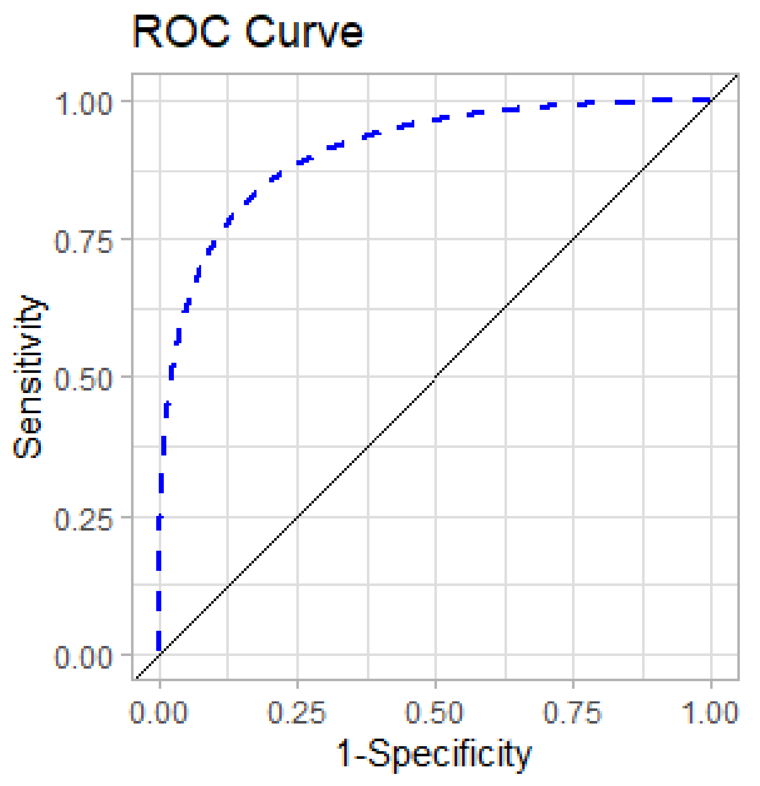
One of the most important evaluation metrics for checking the performance of a binary classification model is the area under the Receiver Operating Characteristics (ROC) curve, called AUC. ROC is a probability curve, with 1-Specificity on the x-axis and Sensitivity on the y-axis (Figure 4). AUC represents the degree or measure of separability between classes. The higher the AUC, the better the model is able to predict the correct class.
Predictive modeling of bathing water quality could be addressed as generally feasible if the two classes can be separated in a way that a satisfying trade-off between recognizing FIB exceedance and avoiding false alarms is obtained. Since our goal is to test the general feasibility of predictive modeling of bathing water quality, and since the dataset we are working with is imbalanced, the best performance alternatives are Informedness and Area under the curve (AUC) [14].
In the step of choosing the best among the different models and tuning the model through a posteriori feature selection, the AUC metric is used because it maximises the overall performance of the model and maximises both Sensitivity and Specificity. Later, when choosing the threshold for the class probability threshold, the decision is made based on the best Informedness.
In the Building the models step, several machine learning models are built [27,28] and for each bacteria the model with the best performance is used for evaluation:
- Random forest is a tree-based model that consists of multiple decision trees. The advantage of random forest is that it reduces the correlation between trees without increasing the variance too much. This is achieved by randomly selecting the input variables for each tree.
- Support vector machines is a nonlinear generalization of linear decision boundaries for classification. It separates classes by producing nonlinear boundaries, thus constructing a linear boundary (hyperplane) that separates classes in a large version of the feature space.
- Artificial neural network is a nonlinear model that simulates the human brain by learning the parameters of the hidden units (simulating neurons) and combining them to form the output layer (decision).
The models are compared using cross-validation [29] according to the chosen metrics in the step of Choosing the best model. Since data collected on the same day may be correlated on a small spatial area [15], predictions might be biased if we perform classical leave-one-out cross-validation (LOOCV) or k-fold cross-validation (k-fold CV). LOOCV and k-fold CV were combined in our leave-one-day-out cross-validation (LODOCV). LODOCV is motivated by Spatial leave-one-out cross-validation (SLOOCV) [30] in which, after selecting a sample, all other samples that are spatially correlated with the removed sample are removed. LODOCV forms folds consisting of samples taken on the same day, resulting in a total of 47 folds. LODOCV is used to compare the performance of different machine learning algorithms and select the one that best fits the data.
2.3.3. Model Tuning and Model Evaluation
After model selection, another set of steps called Model tuning is applied to the best models to achieve the best performance of the models: A posteriori feature selection, i.e., the selection of independent parameters with respect to their importance in the model, and the step Choosing the class probability threshold.
A posteriori feature selection is conducted according to type of the model and the guidelines of [28].Generally, features are selected according to their importance in the model created.
The output of most machine learning classifiers is the probability that a sample belongs to a positive class, and samples are classified as positive if the predicted probability is greater than the threshold, otherwise as negative. The choice of this threshold can have a huge impact on model accuracy, especially for imbalanced datasets [31].
The outputs of the last steps are two models: one model for E. coli and one for intestinal enterococci, which tends to be the best models, according to tests on training data.
In the final step, Model evaluation, the models are further evaluated on holdout data. Outputs of the models are combined into a single model for predicting bathing water quality, as shown in Figure 2.
All parts of the predictive modelling process are performed using the R programming language and its packages: caret for model training and model building, ROSE for balancing data, nnet for artificial neural network creation, randomForest for random forest model creation, and ggplot for visualisation.
3. Results and Discussion
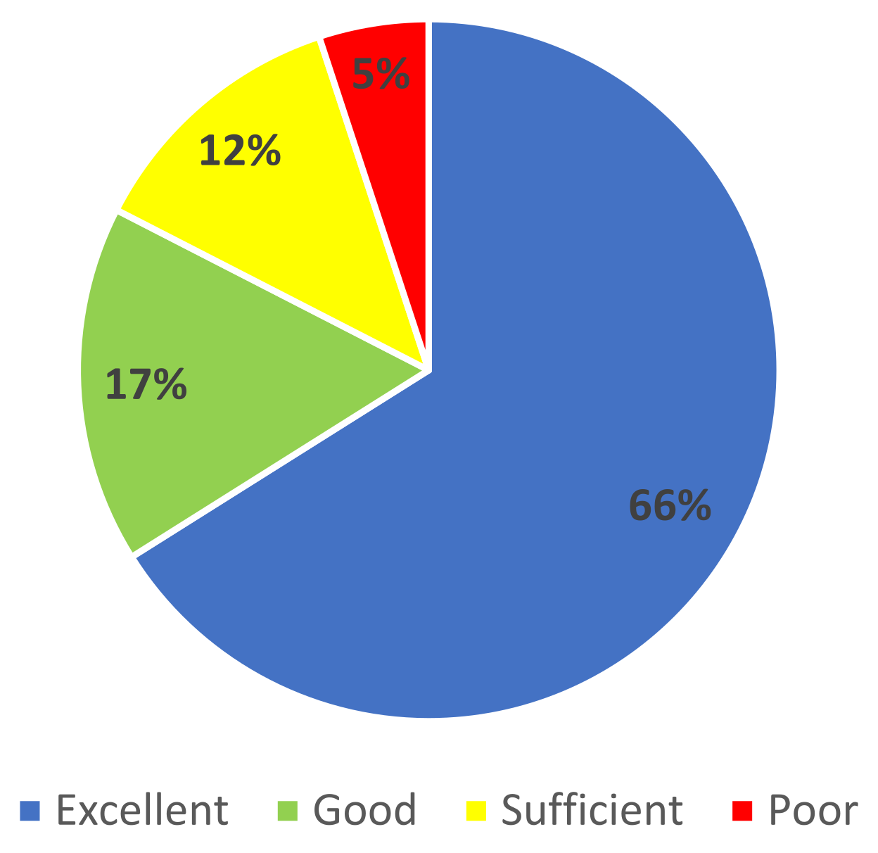
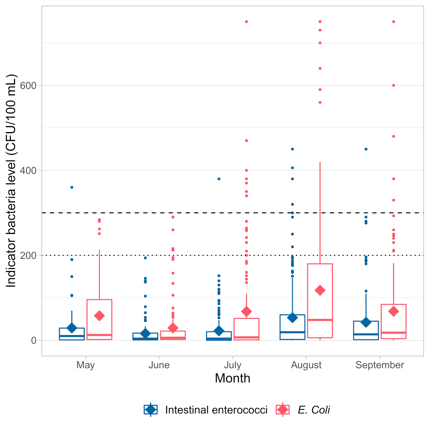
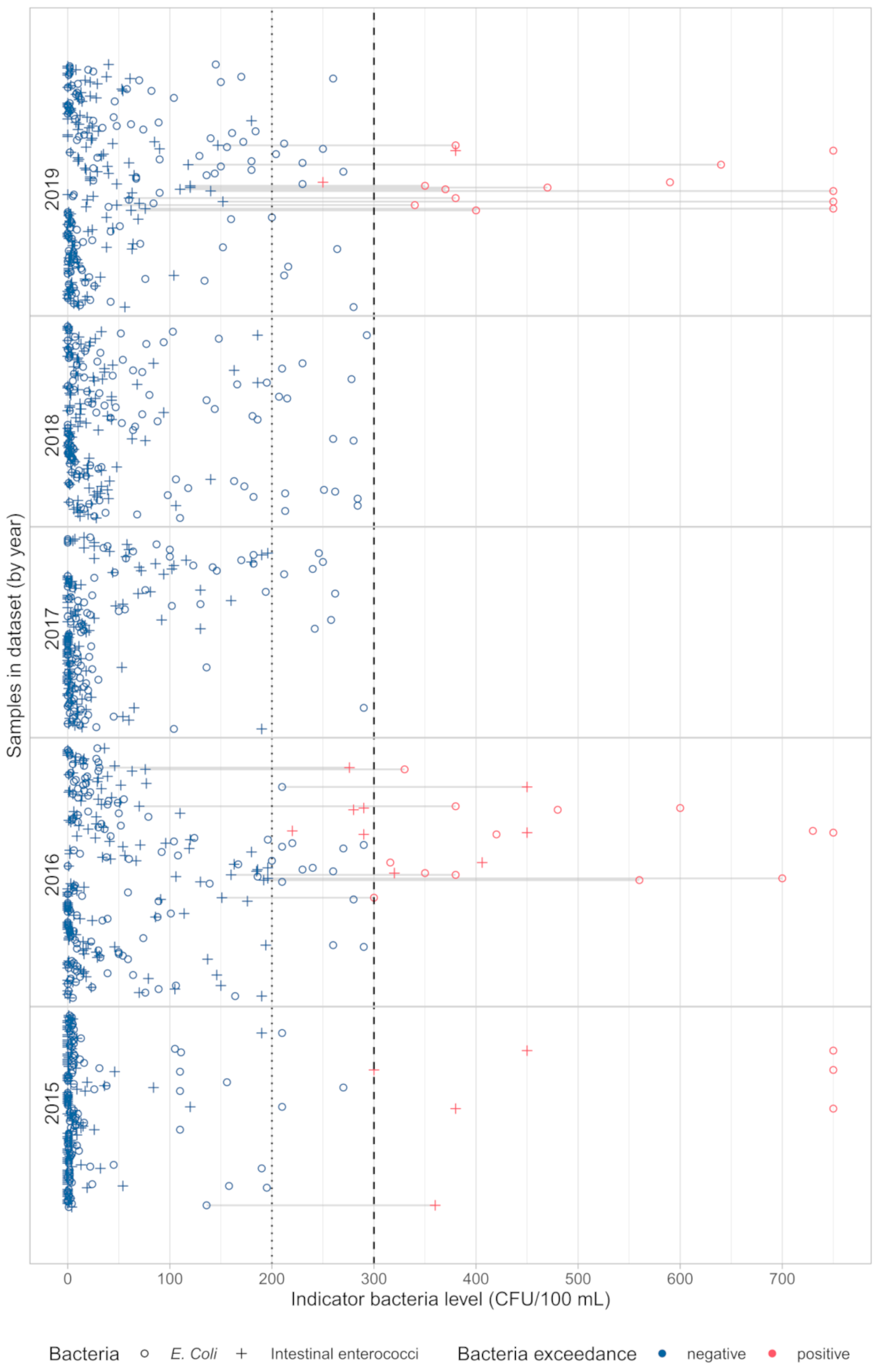
Out of 612 seawater samples collected, 31 (5%) were of poor quality (Figure 5). Most samples (16) had only exceedance of E. coli, three samples had only exceedance of intestinal enterococci, and 12 had exceedance of both FIB. This can be seen in both Figure 6 and Figure 7. Figure 6 depicts variation of both bacteria by months from May to September in the period from 2015 to 2019 for 11 beaches in Kastela. Poor quality is recorded mainly in July, August, and September. Figure 7 shows the variation across years for each sample and also the samples with poor water quality where only one indicator bacteria exceeded the threshold (marked with grey lines).
Of all the poor quality samples, most (23) came from the bathing sites in the eastern part of Kaštela, namely Torac, Kamp and Gojača, indicating that this part of the bay is still subject to higher pollution pressure. Of the 76 (12.4%) samples that showed sufficient quality, 61 (80%) samples showed the exceedance of only one indicator bacteria. Although the bacterial levels are correlated, as expected, it is not uncommon for only one indicator bacteria to exceed the threshold and the other not. One of the main reasons for this is probably the stricter criteria for upper limits for E. coli in Croatian Regulation on Sea Bathing Water Quality [22] compared to the values recommended by European Union Bathing water Dirrective (BWD) [4]. Accordingly, the exceedances are mainly due to increased E. coli levels. This is in line with the results of the analysis 30,000 data collected during the official monitoring of bathing water quality at all Croatian coastal bathing sites in 2015–2018. Of the 779 bathing water samples that were classified in a lower category based on the counts of only one indicator, 59% were classified based on E. coli and 41% based on the counts of intestinal enterococci [32]. Another likely reason is the timing of sampling. Seawater samples for official monitoring are usually collected in the morning so that the samples can be taken to the laboratory and processed the same day. At this time of day, solar radiation, which is the most important factor in reducing FIB, is weaker than during the rest of the day, so it does not have much effect on FIB die-off rates. This is especially true for E. coli, as it is known that this bacteria, like other coliform bacteria, is much more sensitive than intestinal enterococci to the negative effects of environmental factors, especially solar radiation [33,34,35]. If sampling had been conducted in the afternoon, the number of E. coli would likely have decreased more than intestinal enterococci, so water quality exceedances would have been more likely due to increased numbers of intestinal enterococci. This was the motivation to observe faecal indicators separately and to train separate ML models.
The future of predictive modelling of water quality will be even more extensive with more frequent data, by possibly moving from traditional manual methods to technologically advanced methods employing wireless sensor networks for in situ water quality management [36,37]. To be used as support to official monitoring program, predictive models should also satisfy the minimum WHO recommendations that includes: the choice of model and methods of public information dissemination should be reported, the models should meet minimum requirements (including an explained variance of at least 50–60%), and the approach taken should be justifiable and auditable [9].
3.1. Building the Predictive Models
Of the 612 samples collected, 139 are from 2019 and are left as a holdout set, leaving 473 samples for training. It can be seen from Figure 7 that, among all samples in 2019, 13 of them are of poor quality. Only two exceedances of intestinal enterococci are reported, which could affect the results of the evaluation, but still the results of the cross-validation on the training set can give information about the model performance.
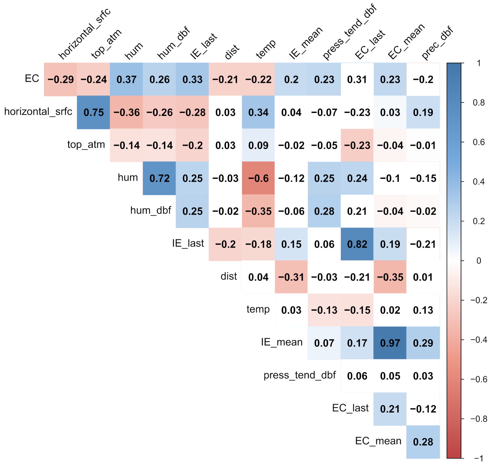
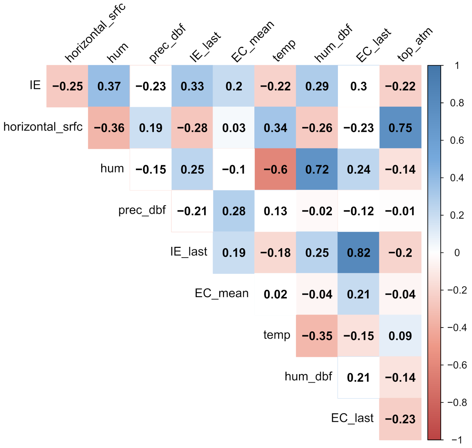
The number of independent parameters is relatively large compared to the size of the dataset, which generally leads to unstable learning. To reduce the number of independent parameters, the correlation with the FIB level on the training set is observed and those with a correlation coefficient (Spearman correlation coefficient [25]) below 0.2 are considered weak and discarded [25,38]. This is done separately for each indicator bacteria, resulting in 12 independent variables for predicting exceedance of E. coli (air temperature—temp, insolation on horizontal surface—horizontal_srfc, top-of-atmosphere insolation—top_atm, pressure tendency on day before—press_tend_dbf, precipitation on day before—prec_dbf, humidity—hum, humidity on day before—hum_dbf, both intestinal enterococci and E. coli count in last sampling—IE_last and EC_last, both the mean number of intestinal enterococci and the mean number of E. coli in the last season—IE_mean and EC_mean and distance to sewage outlet—dist) and nine independent variables for intestinal enterococci (insolation on horizontal surface—horizontal_srfc, top-of- atmosphere insolation—top_atm, precipitation on day before—prec_dbf, humidity—hum, humidity on day before—hum_dbf, both intestinal enterococci and E. coli count in last sampling—IE_last and EC_last, and mean number of E. coli in the last season—EC_mean). Correlation plots of the correlation of 12 features for E. coli and nine for intestinal enterococci are shown in Figure 8 and Figure 9.
The standard data balancing to ratio 50:50 for positive:negative samples leads to a very small dataset in our case (about 40 samples), especially when compared to the dimensionality of the feature space (as many as 12 features for E. coli). Therefore, undersampling is used to bring the dataset to a moderate 10:90 imbalance, as defined by [39]. Furthermore, the metrics of AUC and informedness are used to penalize the majority class preference [16,40]. In addition, at the end, by knowing that dataset is still imbalanced and that all of the models we used are sensitive to it, we adjusted the classification threshold, which is also one of the methods to deal with imbalanced datasets [16].
Each of the models—artificial neural network (ANN), random forest (RF), and support vector machines (SVM)—is validated. Each model is validated by varying the parameters of the model: decay and size for ANN, mtry for RF and degree, and scale and C for SVM as shown in Table 4.
To decide on the best model, the AUC metric is used. For EC_class, the best ANN is obtained for decay = 0.1 and size = 5, the best RF is obtained for mtry = 2, and the best SVM is obtained for degree = 2, scale = 0.1, and C = 1. For IE_class, the best ANN is achieved for decay = 0.1 and size = 5, the best RF for mtry = 2 and the best SVM for degree = 1, scale = 0.001 and C = 0.5.
The ROC for the best models are shown in Figure 10. The ROC represents the overall performance of each model (through different thresholds). AUC values for EC_class prediction for ANN is 0.77, for RF is 0.75, and for SVM is 0.7. AUC values for IE_class prediction for ANN is 0.76, for RF is 0.88, and for SVM is 0.72. Therefore, the best model for EC_class prediction is ANN with decay = 0.1 and size = 5, while the best model for IE_class is RF with mtry = 2. Other metrics can be found in Table 5.
Additional feature selection was performed for the best models for each bacteria. For the ANN model for EC_class, the less important features (according to feature importance—see Table 6a) are discarded one by one and the results (AUC) of the ANNs are compared. The best performance was obtained for ANN with the six most important features (insolation on horizontal surface—horizontal_srfc, top-of-atmosphere insolation—top_atm, humidity— hum, humidity on day before—hum_dbf, intestinal enterococci count in last sampling—IE_last, distance to sewage outlet—dist). For the RF model for IE_class, we manually selected five features by eliminating the least important features that are correlated with other features, since RF is very sensitive to intercorrelations [28]. The RF model with five features (humidity—hum, precipitation on day before—prec_dbf, mean E. coli count in the last season—EC_mean, insolation on horizontal surface—horizontal_srfc, and intestinal enterococci count in last sampling—IE _last) is compared with the model with all features, and it performed better on the training data (see Table 6b).
The default threshold for the class probability threshold is 0.5, but this threshold needs to be adjusted to account for the imbalance in the data that still exist after under-sampling (as described earlier). The trained model is biased towards the negative class, which means that the predicted probability of a positive case is underrated. Therefore, the default threshold for classification by probability is not applicable here.
The threshold with the highest Informedness is taken for each indicator bacteria. For the EC_class, the best threshold is 0.130 and for IE_class 0.172. The cross-validation results for the best models can be found in Table 7.
3.2. Evaluation
The selected models were tested on holdout data using adjusted thresholds. The results of the evaluation on holdout data can be found in Table 8 and Table 9.
The confusion matrix for EC_class (given in the first section of Table 8) shows that the model correctly predicts 11 out of 13 EC_class positives. The model also correctly predicts 109 out of 126 negatives. EC_class is predicted with Informedness 71.1% and F-score 53.7%.
The confusion matrix for IE_class (in the second section of the Table 8) shows that the model correctly predicts 1 out of 2 positives. The model also correctly predicts 127 out of 137 negatives. The confusion matrix for the combined model (in the third section of the Table 8) shows that the model correctly predicts 12 of 13 WQ positives and correctly predicts 100 of 126 negatives. IE _class is predicted with Informedness 92.1% and F-score 15.4%. Combining these two models, the samples are predicted with Informedness 71.7%, F-score 47.1% and an overall Accuracy of 80.6%.
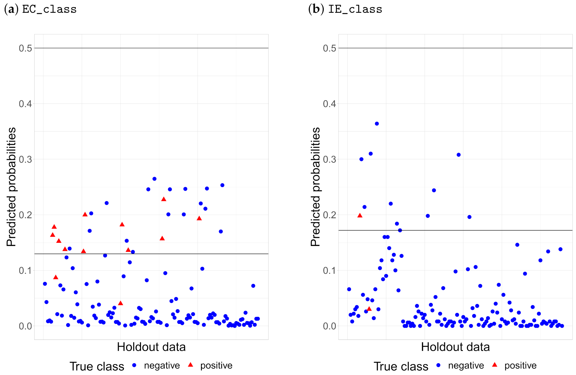
To illustrate the importance of the adjusting probability threshold, samples from the holdout set with default and selected thresholds are shown in Figure 11 for each bacteria. It can be seen that the default threshold classifies all samples in the negative class, whereas the best threshold according to Informedness seems to be a fair trade-off.
Measures of goodness of fit are given in a variety of ways in related work, and some of them are not even measurable for the models used in this paper (such as the measure of explained variance). However, when we compare the results presented in this paper with related works that are most similar to ours, we can see that the performance of our models is much better. Although related works report high specificity: 88% and 94% for [11], from 85% up to 95% for [12] and 98% [13], they achieved very low sensitivity: 18% and 28% for [11], from 37% up to 56% for [12] and 11.2% [13], meaning that a small amount of poor water quality is correctly classified as poor. Informedness calculated based on the Sensitivity and Specificity reported in related works are: 12% and 16% for [11], from 22% up to 51% for [12] and 0.92% [13], which is much lower than the Informedness of 71.7% obtained by our approach.
4. Conclusions
The use of data from official monitoring of coastal waters in Kaštela bay, collected during five bathing seasons, resulted in the building of predictive models with acceptable properties. Testing of several models showed no silver bullet model, and led to the selection of different models for the two different indicator bacteria, the ANN (Neural network) model for E. coli and the RF (Random forest) model for intestinal enterococci. This is likely the result of the different fate of these indicators after entering the marine environment, the different resistance to the same environmental factors and consequently the different culturability. Both models showed acceptable performance characteristics when validated, with an overall accuracy of 80.6% and an informedness of 71.7%. With the properties achieved, the model can be successfully used as a supplement to regular monitoring. This means that the model itself, like other models, cannot and should not be the only tool for monitoring bathing water quality, but that classical monitoring must still be carried out. First, because the model still needs to be filled with data to check whether the water quality estimates are correct or whether the predictor variables have changed, the model needs to be updated. Once built, the predictive model is an easy-to-use tool that only has to be fed by current data of the most important environmental features (model predictors). Secondly, the classical methods for determining the concentration of indicator bacteria in bathing water are still the only relevant and legally acceptable methods that provide information on the actual state of bathing water quality. Therefore, as there is not yet a legal basis for using the model to produce official bathing water quality assessments, the model can be used to warn bathers of a possible deterioration in bathing water quality. It can also be used as a tool for official laboratories involved in bathing water quality monitoring to indicate the need for additional sampling in the period between regular sampling when predicted bathing water quality is not satisfactory. (e.g., in case of short-term pollution). The main problem with this modelling approach is to record a sufficient number of cases where bathing water quality is poor (exceedances) so that the data are more balanced, i.e., the proportion of poor samples is not too low. More exceedance data would also result in a greater number of environmental conditions that lead to poor bathing water quality. This is particularly true for intestinal enterococci, as due to the inappropriate defined criteria for thresholds for two indicators in the Croatian legislation, most exceedances are due to the increased E. coli levels. Another problem is the relatively long period of time required to collect a sufficient number of useful data. More frequent sampling over a larger area would be hardly feasible for official monitoring due to the high costs, resources, and technical limitations. Since bathing sites that occasionally exhibit ‘poor’ water quality may be detected during regular monitoring, as is the case in this study, better data could be provided if the monitoring program is improved on a spatial and temporal basis only at such sites. This would mean sampling such areas more frequently, including in the afternoon, and establishing additional sampling sites to better monitor the distribution of pollution. In this way, the time taken to collect the required amount of useful data could be significantly reduced. In addition to ’normal’ weather conditions, sampling should also be carried out in a range of weather conditions, from tides to severe weather such as rain and wind from the direction of the identified source of pollution. With new data, the predictive modelling process described could be modified and new procedures and methods could be used.
Author Contributions
Conceptualization, I.N.K., T.M. and S.J.; methodology, I.N.K. and D.D.; software, D.D. and I.N.K.; validation, D.D., I.N.K. and S.J.; formal analysis, D.D., I.N.K. and T.M.; investigation, D.D.; resources, D.I.; data curation, T.M.; writing—original draft preparation, D.D. and I.N.K.; writing—review and editing, I.N.K., S.J. and T.P.; visualization, D.D. and I.N.K.; supervision, S.J. and I.N.K.; project administration, I.N.K. and S.J.; funding acquisition, S.J. All authors have read and agreed to the published version of the manuscript.
Funding
This research was funded by the Croatian Science Foundation, Grant No. IP-2020-02-1880 (project Eurobath).
Institutional Review Board Statement
Not applicable.
Informed Consent Statement
Not applicable.
Data Availability Statement
The data presented in this study are available on request from the corresponding author. The data are not publicly available because they come from the official Croatian monitoring of coastal bathing waters.
Acknowledgments
The authors would like to thank their colleagues from the Teaching Institute of Public Health of Split-Dalmatia County, who carried out the official monitoring and obtained bathing water quality data in the area of Kaštela Bay.
Conflicts of Interest
The authors declare no conflict of interest. The funders had no role in the design of the study; in the collection, analyses, or interpretation of data; in the writing of the manuscript, or in the decision to publish the results.
Sample Availability
Not applicable.
Abbreviations
The following abbreviations are used in this manuscript:
| BWD | Bathing Water Directive |
| FIB | Faecal Indicator Bacteria |
| RF | Random Forest |
| ANN | Neural Network |
| ROC | Receiver Operating Characteristics |
| AUC | Area Under the Curve |
| LOOCV | Leave-One-Out Cross Validation |
| LODOCV | Leave-One-Day-Out Cross Validation |
| SLOOCV | Spatial Leave-One-Out Cross-Validation |
| SVM | Support Vector Machines |
References
- Preißler, S. Evaluation of the quality of European coastal water by German tourists. Coast. Chang. South. Balt. Sea Reg. Coastline Rep. 2009, 12, 177–186. [Google Scholar]
- Dodds, R.; Holmes, M.R. Education and certification for beach management: Is there a difference between residents versus visitors? Ocean Coast. Manag. 2018, 160, 124–132. [Google Scholar] [CrossRef]
- Schuhmann, P.; Skeete, R.; Waite, R.; Bangwayo-Skeete, P.; Casey, J.; Oxenford, H.A.; Gill, D.A. Coastal and Marine Quality and Tourists’ Stated Intention to Return to Barbados. Water 2019, 11, 1265. [Google Scholar] [CrossRef] [Green Version]
- Directive 2006/7/EC of the European Parliament and of the Council of 15 February 2006 concerning the management of bathing water quality and repealing Directive 76/160/EEC. Off. J. Eur. Union 2006, L 64, 37–51.
- Publications Office of the European Union. European Bathing Water Quality in 2015, EEA Report No 9/2016; Publications Office of the European Union: Luxembourg, 2016. [Google Scholar]
- Leecaster, M.K.; Weisberg, S.B. Effect of Sampling Frequency on Shoreline Microbiology Assessments. Mar. Pollut. Bull. 2001, 42, 1150–1154. [Google Scholar] [CrossRef]
- World Health Organization. Guidelines for Safe Recreational Water Environments: Coastal and Fresh Waters; World Health Organization: Geneva, Switzerland, 2003; Volume 1. [Google Scholar]
- World Health Organization. Addendum to the WHO Guidelines for Safe Recreational Water Environments: Coastal and Fresh Waters: List of Agreed Updates; World Health Organization: Geneva, Switzerland, 2009; Volume 1. [Google Scholar]
- World Health Organization. WHO Recommendations on Scientific, Analytical and Epidemiological Developments Relevant to the Parameters for Bathing Water Quality in the Bathing Water Directive (2006/7/EC); World Health Organization: Geneva, Switzerland, 2018. [Google Scholar]
- de Brauwere, A.; Ouattara, N.K.; Servais, P. Modeling Fecal Indicator Bacteria Concentrations in Natural Surface Waters: A Review. Crit. Rev. Environ. Sci. Technol. 2014, 44, 2380–2453. [Google Scholar] [CrossRef] [Green Version]
- Thoe, W.; Gold, M.; Griesbach, A.; Grimmer, M.; Taggart, M.L.; Boehm, A.B. Predicting water quality at Santa Monica Beach: Evaluation of five different models for public notification of unsafe swimming conditions. Water Res. 2014, 67, 105–117. [Google Scholar] [CrossRef]
- Thoe, W.; Choi, K.W.; Lee, J.H.W. Predicting ’very poor’ beach water quality gradings using classification tree. J. Water Health 2016, 14, 97–108. [Google Scholar] [CrossRef] [Green Version]
- Lucius, N.; Rose, K.; Osborn, C.; Sweeney, M.E.; Chesak, R.; Beslow, S.; Schenk, T. Predicting E. coli concentrations using limited qPCR deployments at Chicago beaches. Water Res. X 2019, 2, 100016. [Google Scholar] [CrossRef]
- Ward Powers, D.M. Evaluation: From precision, recall and f-measure to roc, informedness, markedness & correlation. J. Mach. Learn. Technol. 2011, 2, 37–63. [Google Scholar]
- A Ramezan, C.; A Warner, T.; E Maxwell, A. Evaluation of Sampling and Cross-Validation Tuning Strategies for Regional-Scale Machine Learning Classification. Remote Sens. 2019, 11, 185. [Google Scholar] [CrossRef] [Green Version]
- Fernández, A.; García, S.; Galar, M.; Prati, R.C.; Krawczyk, B.; Herrera, F. Learning from Imbalanced Data Sets; Springer International Publishing: Berlin/Heidelberg, Germany, 2018. [Google Scholar]
- Valverde-Albacete, F.J.; Peláez-Moreno, C. 100% classification accuracy considered harmful: The normalized information transfer factor explains the accuracy paradox. PLoS ONE 2014, 9, e84217. [Google Scholar] [CrossRef] [Green Version]
- Avila, R.; Horn, B.; Moriarty, E.; Hodson, R.; Moltchanova, E. Evaluating statistical model performance in water quality prediction. J. Environ. Manag. 2018, 206, 910–919. [Google Scholar] [CrossRef]
- Ahmed, U.; Mumtaz, R.; Anwar, H.; Shah, A.A.; Irfan, R.; García-Nieto, J. Efficient Water Quality Prediction Using Supervised Machine Learning. Water 2019, 11, 2210. [Google Scholar] [CrossRef] [Green Version]
- Zore-Armanda, M. Some dynamic and hydrographic properties of the Kaštela Bay. Acta Adriat. 1980, 21, 55–74. [Google Scholar]
- Kuspilić, G.; Lusic, J.; Milun, V.; Mandic, J.; Nincevic Gladan, Z.; Krstulovic, N.; Solic, M.; Marijanović Rajcic, M.; Surmanovic, D.; Gonzalez-Fernandez, D.; et al. Temporal changes in chemical and biological properties of Kastela Bay. In Proceedings of the Hrvatska Konferencija o Vodama, Hrvatske Vode na Investicijskom Valu, Zagreb, Croatia, January 2015. [Google Scholar]
- Official Gazette of the Republic of Croatia “Narodne Novine” 73/2008. Regulation on Sea Bathing Water Quality; The Government of The Republic of Croatia: Zagreb, Croatia, 2008.
- Jozić, S.; Vukić Lušić, D.; Ordulj, M.; Frlan, E.; Cenov, A.; Diković, S.; Kauzlarić, V.; Fiorido Đurković, L.; Stilinović Totić, J.; Ivšinović, D.; et al. Performance characteristics of the temperature-modified ISO 9308-1 method for the enumeration of Escherichia coli in marine and inland bathing waters. Mar. Pollut. Bull. 2018, 135, 150–158. [Google Scholar] [CrossRef]
- ISO Central Secretary. Water Quality—Detection and Enumeration of Intestinal Enterococci—Part 2: Membrane Filtration Method; Standard ISO 7899-2:2000; International Organization for Standardization: Geneva, Switzerland, 2000. [Google Scholar]
- Kuhn, M.; Johnson, K. Applied Predictive Modeling; Springer: New York, NY, USA, 2013. [Google Scholar]
- Tyagi, S.; Mittal, S. Sampling Approaches for Imbalanced Data Classification Problem in Machine Learning; Lecture Notes in Electrical Engineering; Springer: Cham, Switzerland, 2020; Volume 597, pp. 209–221. [Google Scholar] [CrossRef]
- James, G.; Witten, D.; Hastie, T.; Tibshirani, R. An Introduction to Statistical Learning; Springer: New York, NY, USA, 2021. [Google Scholar] [CrossRef]
- Hastie, T.; Tibshirani, R.; Friedman, J. The Elements of Statistical Learning; Springer Series in Statistics; Springer: New York, NY, USA, 2001. [Google Scholar]
- Arlot, S.; Celisse, A. A survey of cross-validation procedures for model selection. Stat. Surv. 2010, 4, 40–79. [Google Scholar] [CrossRef]
- Le Rest, K.; Pinaud, D.; Monestiez, P.; Chadoeuf, J.; Bretagnolle, V. Spatial leave-one-out cross-validation for variable selection in the presence of spatial autocorrelation. Glob. Ecol. Biogeogr. 2014, 23, 811–820. [Google Scholar] [CrossRef] [Green Version]
- Freeman, E.A.; Moisen, G.G. A comparison of the performance of threshold criteria for binary classification in terms of predicted prevalence and kappa. Ecol. Model. 2008, 217, 48–58. [Google Scholar] [CrossRef]
- Jozić, S. Appropriateness of the limit values for microbiological indicators of coastal bathing water quality set out in the Regulation on sea bathing water quality. In Proceedings of the Presented at XXV Working Meeting of County Public Health Institutes, Administrative Departments and Institutes Responsible for Environmental Protection, Physical Planning, Construction, Communal Economy, Sustainable Development and Maritime Affairs of the Adriatic Area, Brijuni, Croatia, 29 April 2018. [Google Scholar]
- Fujioka, R.S.; Hashimoto, H.H.; Siwak, E.B.; Young, R.H. Effect of sunlight on survival of indicator bacteria in seawater. Appl. Environ. Microbiol. 1981, 41, 690–696. [Google Scholar] [CrossRef] [PubMed] [Green Version]
- Sinton, L.W.; Davies-Colley, R.J.; Bell, R.G. Inactivation of enterococci and faecal coliforms from sewage and meatworks effluents in seawater chambers. Appl. Environ. Microbiol. 1994, 60, 2040–2048. [Google Scholar] [CrossRef] [PubMed] [Green Version]
- Davies-Colley, R.J.; Bell, R.G.; Donnison, A.M. Sunlight Inactivation of Enterococci and Fecal Coliforms in Sewage Effluent Diluted in Seawater. Appl. Environ. Microbiol. 1994, 60, 2049–2058. [Google Scholar] [CrossRef] [Green Version]
- Adu-Manu, K.S.; Tapparello, C.; Heinzelman, W.; Katsriku, F.A.; Abdulai, J.D. Water quality monitoring using wireless sensor networks: Current trends and future research directions. ACM Trans. Sens. Netw. 2017, 13, 1–41. [Google Scholar] [CrossRef] [Green Version]
- Muharemi, F.; Logofătu, D.; Leon, F. Machine learning approaches for anomaly detection of water quality on a real-world data set. J. Inf. Telecommun. 2019, 3, 294–307. [Google Scholar] [CrossRef] [Green Version]
- Chandrashekar, G.; Sahin, F. A survey on feature selection methods. Comput. Electr. Eng. 2014, 40, 16–28. [Google Scholar] [CrossRef]
- Japkowicz, N.; Japkowicz, N.; Stephen, S. The class imbalance problem: A systematic study. Intell. Data Anal. 2002, 6, 429–449. [Google Scholar] [CrossRef]
- Luque, A.; Carrasco, A.; Martín, A.; de las Heras, A. The impact of class imbalance in classification performance metrics based on the binary confusion matrix. Pattern Recognit. 2019, 91, 216–231. [Google Scholar] [CrossRef]
Figure 1.
Map of Kaštela Bay and bathing sites where samples were taken.

Figure 2.
Scheme of the binary classification model for bathing water quality prediction.

Figure 3.
Predictive modelling process for bathing water quality.

Figure 4.
Receiver Operating Characteristics (ROC) curve (blue).

Figure 5.
The percentage of bathing water quality categories of all samples collected from 11 beaches in Kaštela in 2015–2019.
Figure 5.
The percentage of bathing water quality categories of all samples collected from 11 beaches in Kaštela in 2015–2019.

Figure 6.
Summary of FIB levels grouped by months. The blue color represents intestinal enterococci and the red color E. coli. The line represents median and diamond shape mean values. The dashed line is the threshold for E. coli exceedance and the dotted line is the threshold for intestinal enterococci.

Figure 7.
FIB level of samples from dataset, sorted by timestamp. Each sample is represented by a line, the circle being CFU/100 mL of E. coli and plus being CFU/100 mL of intestinal enterococci. Samples marked red represents poor quality.
Figure 7.
FIB level of samples from dataset, sorted by timestamp. Each sample is represented by a line, the circle being CFU/100 mL of E. coli and plus being CFU/100 mL of intestinal enterococci. Samples marked red represents poor quality.

Figure 8.
Correlation plot of parameters with strongest correlation with E. coli. Description of features is given in Table 2.
Figure 8.
Correlation plot of parameters with strongest correlation with E. coli. Description of features is given in Table 2.

Figure 9.
Correlation plot of parameters with strongest correlation with intestinal enterococci. Description of features is given in Table 2.
Figure 9.
Correlation plot of parameters with strongest correlation with intestinal enterococci. Description of features is given in Table 2.

Figure 10.
ROC of different classifiers (ANN, RF, and SVM) for EC_class and IE_class prediction.

Figure 11.
Classification probabilities of samples and probabilities thresholds. Red triangles represent the actual positive class and blue dots the actual negative class. Horizontal lines represent a default classification threshold of 0.5 and adjusted thresholds of 0.130 for EC_class and 0.172 for IE_class.


Table 1.
Standards for bathing water quality after each sampling.
| Bathing Water Quality | |||||
|---|---|---|---|---|---|
| Excellent | Good | Sufficient | Poor | ||
| Bacteria | Intestinal enterococci | ≤60 | 61–100 | 101–200 | >200 |
| Escherichia coli | ≤100 | 101–200 | 201–300 | >300 | |
Table 2.
Overview of features in data set. The first four features describing the sample are excluded from modelling, and the last three features (EC_class, E_class and WQ) are the ones to be modelled (dependent variables). The other 35 features are used in modelling as independent variables.
Table 2.
Overview of features in data set. The first four features describing the sample are excluded from modelling, and the last three features (EC_class, E_class and WQ) are the ones to be modelled (dependent variables). The other 35 features are used in modelling as independent variables.
| Feature Name | Description |
|---|---|
| loc | Sampling site (latitude and longitude) |
| t | Sampling timestamp |
| EC | E. coli count (CFU/100 mL) |
| IE | Intestinal enterococci count (CFU/100 mL) |
| EC_last | E. coli count in last sampling (CFU/100 mL) |
| EC_mean | Mean E. coli count in last bathing season (CFU/100 mL) |
| IE_last | Intestinal enterococci count in last sampling (CFU/100 mL) |
| IE_mean | Mean intestinal enterococci count in last bathing season (CFU/100 mL) |
| sal | Salinity |
| sea_temp | Seawater temperature (°C) |
| wind_cat | Wind (yes/no) |
| prec_cat | Precipitation (present/moderate/absent) |
| weather | Weather description (cloudy/partly cloudy/sunny) |
| high | Highest daily sea level (m) |
| low | Lowest daily sea level (m) |
| dist | Distance to sewage outlet (m) |
| temp | Air temperature (°C) |
| temp_dbf | Air temperature day before (°C) |
| hum | Humidity (%) |
| hum_dbf | Humidity day before (%) |
| press | Pressure at weather station level (mm of mercury) |
| press_dbf | Pressure at weather station level day before (mm of mercury) |
| press_tend | Pressure tendency (mm of mercury) |
| press_tend_dbf | Pressure tendency day before (mm of mercury) |
| press_rel | Relative pressure at sea level (mm of mercury) |
| press_rel_dbf | Relative pressure at sea level day before (mm of mercury) |
| wind_sp | Wind speed (m/s) |
| wind_sp_dbf | Wind speed day before (m/s) |
| wind_dir | Wind direction (compass angle) |
| wind_dir_dbf | Wind direction day before (compass angle) |
| cloud | Cloud coverage (%) |
| cloud_dbf | Cloud coverage day before (%) |
| prec | Precipitation in last 24 h (mm) |
| prec_dbf | Precipitation in last 24 h day before (mm) |
| thermal_infrared | Downward Thermal Infrared (Longwave) Radiative Flux (MJ/m/day) |
| horizontal_srfc | All Sky Insolation Incident on a Horizontal Surface (MJ/m/day) |
| top_atm | Top-of-atmosphere Insolation (MJ/m/day) |
| clearness | Insolation Clearness Index |
| overnights | Number of tourist overnights |
| EC_class | Exceedance of E. coli according to poor quality threshold—(positive/negative) |
| IE_class | Exceedance of intestinal enterococci according to poor quality threshold—(positive/negative) |
| WQ | Exceedance of at least one of bacteria: E. coli and/or intestinal enterococci—(positive/negative) |
Table 3.
Confusion matrix format for binary classification, with depicted true positives (TP), false negatives (FN), false positives (FP), and true negatives (TN) cases.
Table 3.
Confusion matrix format for binary classification, with depicted true positives (TP), false negatives (FN), false positives (FP), and true negatives (TN) cases.
| Actual Value | |||
|---|---|---|---|
| Positive | Negative | ||
| Prediction | positive | TP | FP |
| negative | FN | TN | |
Table 4.
Tuning parameters for ANN, RF, and SVM for EC_class and IE_class.
| EC_class | IE_class | ||
|---|---|---|---|
| ANN | decay | 0, 0.1, 0.0001 | |
| size | 1, 3, 5 | ||
| RF | mtry | 2, 7, 12 | 2, 5, 9 |
| SVM | degree | 1, 2, 3 | |
| scale | 0.001, 0.01, 0.1 | ||
| C | 0.25, 0.5, 1 | ||
Table 5.
Cross validation results of several models before tuning parameters.
| Metrics for Default Threshold (0.5) | ||||||
|---|---|---|---|---|---|---|
| Model | AUC | Sensitivity | Specificity | Informedness | F-Score | |
| EC_class | ANN * | 0.770 | 0.267 | 0.964 | 0.231 | 0.333 |
| RF ** | 0.754 | 0.067 | 0.978 | 0.045 | 0.105 | |
| SVM | 0.704 | 0.000 | 0.978 | −0.022 | NaN | |
| IE_class | ANN * | 0.759 | 0.385 | 0.963 | 0.348 | 0.455 |
| RF ** | 0.875 | 0.077 | 0.982 | 0.059 | 0.125 | |
| SVM | 0.718 | 0.000 | 0.972 | −0.028 | NaN | |
* decay = 0.1, size = 5; ** mtry = 2; + degree = 2, scale = 0.1, C = 1; ++ degree = 1, scale = 0.001, C = 0.5; +++ can’t be calculated because model classifies all samples as negatives.
Table 6.
A posteriori feature selection for best classification models for each of bacteria. (a) feature importance for best ANN for EC_class; (b) selected features for best RF for IE_class based on their correlation with other features. In groups of highly correlated features (≥0.5), the one with the highest correlation with IE is selected.
| (a) | |
| Feature | Importance |
| horizontal_srfc | 100.00 |
| top_atm | 95.716 |
| hum | 40.622 |
| hum_dbf | 38.468 |
| IE_last | 38.054 |
| dist | 32.206 |
| temp | 19.240 |
| IE_mean | 13.313 |
| pres_tend_dbf | 8.544 |
| EC_last | 7.422 |
| EC_mean | 3.132 |
| prec_dbf | 0.000 |
| (b) | |
| Feature | Highly corr. with |
| horizontal_srfc | top_atm |
| hum | hum_dbf, temp |
| prec_dbf | - |
| IE_last | EC_last |
| EC_mean | - |
| temp | hum |
| hum_dbf | hum |
| EC_last | IE_last |
| top_atm | horizontal_srfc |
Table 7.
Cross validation results of best models (after tuning the parameters—features and probability thresholds).
Table 7.
Cross validation results of best models (after tuning the parameters—features and probability thresholds).
| Metrics for Best Thresholds | |||||
|---|---|---|---|---|---|
| AUC | Sensitivity | Specificity | Informedness | F-Score | |
| ANN forEC_class | 0.919 | 0.933 | 0.899 | 0.833 | 0.333 |
| RF forIE_class | 0.891 | 0.846 | 0.881 | 0.727 | 0.200 |
Table 8.
Confusion matrices for binary classification of E. coli (EC_class), intestinal enterococci (IE_class), and combined model (WQ).
Table 8.
Confusion matrices for binary classification of E. coli (EC_class), intestinal enterococci (IE_class), and combined model (WQ).
| Actual Value | |||
|---|---|---|---|
| Positive | Negative | ||
| PredictedEC_class | positive | 11 | 17 |
| negative | 2 | 109 | |
| PredictedIE_class | positive | 1 | 10 |
| negative | 1 | 127 | |
| PredictedWQ | positive | 12 | 26 |
| negative | 1 | 100 | |
Table 9.
Various metrics for EC_class, IE_class, and WQ prediction.
| Accuracy | Sensitivity | Specificity | Informedness | F-Score | |
|---|---|---|---|---|---|
| EC_class model | 0.863 | 0.846 | 0.865 | 0.711 | 0.537 |
| IE_class model | 0.921 | 0.500 | 0.927 | 0.427 | 0.154 |
| WQ model | 0.806 | 0.923 | 0.794 | 0.717 | 0.471 |
Publisher’s Note: MDPI stays neutral with regard to jurisdictional claims in published maps and institutional affiliations. |
© 2021 by the authors. Licensee MDPI, Basel, Switzerland. This article is an open access article distributed under the terms and conditions of the Creative Commons Attribution (CC BY) license (https://creativecommons.org/licenses/by/4.0/).
Share and Cite
MDPI and ACS Style
Džal, D.; Kosović, I.N.; Mastelić, T.; Ivanković, D.; Puljak, T.; Jozić, S. Modelling Bathing Water Quality Using Official Monitoring Data. Water 2021, 13, 3005. https://doi.org/10.3390/w13213005
AMA Style
Džal D, Kosović IN, Mastelić T, Ivanković D, Puljak T, Jozić S. Modelling Bathing Water Quality Using Official Monitoring Data. Water. 2021; 13(21):3005. https://doi.org/10.3390/w13213005
Chicago/Turabian StyleDžal, Daniela, Ivana Nižetić Kosović, Toni Mastelić, Damir Ivanković, Tatjana Puljak, and Slaven Jozić. 2021. "Modelling Bathing Water Quality Using Official Monitoring Data" Water 13, no. 21: 3005. https://doi.org/10.3390/w13213005
Note that from the first issue of 2016, this journal uses article numbers instead of page numbers. See further details here.