
Effect of Surface Water Level Fluctuations on the Performance of Near-Bank Managed Aquifer Recharge from Injection Wells

1
School of Water Conservancy Engineering, Zhengzhou University, Zhengzhou 450001, China
2
State Key Laboratory of Hydrology-Water Resources and Hydraulic Engineering, Nanjing Hydraulic Research Institute, Nanjing 210098, China
3
Key Laboratory of Groundwater Resources and Environment, Jilin University, Ministry of Education, Changchun 130021, China
4
School of Geosciences, University of Aberdeen, Aberdeen AB24 3FX, UK
5
The Fifth Institute of Resources and Environment Survey of Henan Province, Xinxiang 450001, China
*
Authors to whom correspondence should be addressed.
Water 2021, 13(21), 3013; https://doi.org/10.3390/w13213013
Submission received: 27 September 2021
/
Revised: 21 October 2021
/
Accepted: 25 October 2021
/
Published: 27 October 2021
(This article belongs to the Section Hydrogeology)
Abstract
:Managed aquifer recharge operations are often conducted in near-bank areas to regulate water resources or reduce seawater intrusion. Yet little is known about the influence of surface water level fluctuations at different temporal scales on MAR performance. A generalized conceptual model was developed based on an investigation site in Western China as a basis to simulate the response surface water level fluctuations on the water table, artificially recharged water lens (formed by the artificially recharged water), groundwater flow paths and average travel times (which is an important control on how quickly contaminants are flushed out of aquifers), and the discharge of the artificially recharged aquifer during the surface water level fluctuation. The results showed a fluctuating groundwater table in the artificially recharged near-bank aquifer under the influence of surface water level fluctuations. The peak values of the increment of the groundwater table induced by artificial recharge decreased with the increase of the period and amplitude of surface water level fluctuation, but the trough values of the increment of water table increases with that. The penetration depth of surface water into the aquifer with a fluctuating surface water level leads to a decreasing increment of the groundwater table which follows a power law. The fluctuating surface water level leads to dynamic changes of artificially recharged water lens morphology and a thinner artificially recharged water lens. A mixing zone of recharged water and ambient water could be found in the artificially recharged near-bank area, which is expected to lead to modifications in the geochemical conditions in the artificially recharged near-bank aquifer. A longer period of surface water level fluctuation leads to a longer average travel time, but the larger penetration depth of surface water and amplitude lead to a shorter average travel time. The peak discharge of the near-bank aquifer was found to decrease with the period of surface water level fluctuation, but it increases with penetration depth and amplitude. This study is important in providing insights into the performance of near-bank managed aquifer recharge with respect to surface water level fluctuation.
1. Introduction
Managed aquifer recharge (MAR) is an effective method of increasing the quantities of groundwater resources by capturing seasonally or intermittently available excess surface water artificially [1,2], which has been implemented in many regions around the word, such as the United States [3], Australia [4,5], Europe [6], China [1] and elsewhere. MARs are conducted to augment groundwater resources in arid and semi-arid areas [1], reducing seawater intrusion [7] and land subsidence [8]. For example, MARs are needed in some regions of the arid areas in western China to regulate water resources because the surface water is mostly recharged by precipitation and melt water from ice and snow and floods always occurs in spring and summer, while drought occurs in autumn and winter [1,9]. Apart from suitability based on soil properties, the feasibility of MARs is always governed by source water. Thus, MARs are often constructed in rivers’ near-bank areas [10,11,12,13] to enhance groundwater quantity where they can reduce the diversion cost of source water that is used for artificial recharge. Similarly, MAR systems have also been constructed in near-shore areas in order to reduce sea-water intrusion. However, surface water levels (SWLs) are typically subject to large temporal variations on different timescales due to natural drivers and anthropogenic interference [14,15,16,17], and the performance of near-bank MARs subject to surface water level fluctuations has received little attention.
Groundwater over-extraction and depletion associated with economic development, population growth, increasing urbanization and irrigation affects many countries, and has induced a series of indirect environmental geological problems, e.g., land subsidence and sea water intrusion, during the past few decades [18,19,20]. Thus, MARs are increasingly promoted as an effective way to replenish aquifers through various approaches such as e.g., aquifer storage and recovery (ASR) [10], aquifer storage transfer and recovery (ASTR) [21], infiltration basins and injection wells [5,22], vadose zone infiltration wells [2], and streambed channel modifications [23]. In the past, most MAR studies were conducted to investigate the clogging of wells and aquifers [24,25], efficiency of artificial recharge [2], recovery efficiency (RE) [26] and groundwater quality changes [10]. These studies typically used physical experiments, numerical simulations and/or field investigations in which static surface water boundary conditions were normally considered.
Traditionally, the investigations on groundwater dynamics and SW–GW (surface water and ground water) interactions in response to surface water level fluctuations fall under two categories, that is the groundwater flow and mass transport driven by sea water level and the interaction of GW–SW in inland zones. Much more attention has been given to the groundwater flow and associated mass transport in response to sea water level variations in near-shore zones. Including low-frequency tides and high frequency waves [16,27,28,29,30,31,32,33,34]. All these studies showed that a water table driven by sea level fluctuations is asymmetrical with a quick rising phase and slow falling phase in both confined and unconfined aquifers [17]. For example, Yu et al. [35] showed the response of seawater intrusion and seawater retreat to the inland water table variations was affected by tidal conditions. Geng et al. [36] showed the spreading coefficient of the solute plume in a beach aquifer shows a very dynamic response to tides. When compared with near-shore zones, the SW–GW interactions driven by surface water fluctuations in inland zones have been relatively less considered and few studies have examined hyporheic exchange and groundwater hydraulic subjected to flood pulses [37,38,39,40]. These studies demonstrated that the groundwater pressure induced by flood pulse lagged with the distance from the stream due to soil damping, which can enhance the water and transport of solutes flux between stream and aquifer [40,41,42]. Sensitivity analysis of stream–aquifer exchanges to in-stream water level fluctuations has been investigated by Baratelli et al. [43], which showed the importance of accounting for river stage fluctuations in the modelling of regional hydro-systems. Modelling from Gu et al. [44] demonstrated that high biogeochemical activities occurred at the near-stream riparian zone during stage fluctuation, which has been verified through field observations.
The specific objectives of this paper are to examine groundwater flow behavior under the influence of both artificial recharge through injection wells and fluctuating SWL using numerical simulation-based site investigations. Based on the numerical model outputs, the effects of SWL fluctuations on the water table, artificially recharged water lens, groundwater flow paths and travel times of artificially recharged water, and the discharge of the near bank aquifer to surface water were analyzed and quantified using regression models.
2. Methodology
2.1. Site Investigations
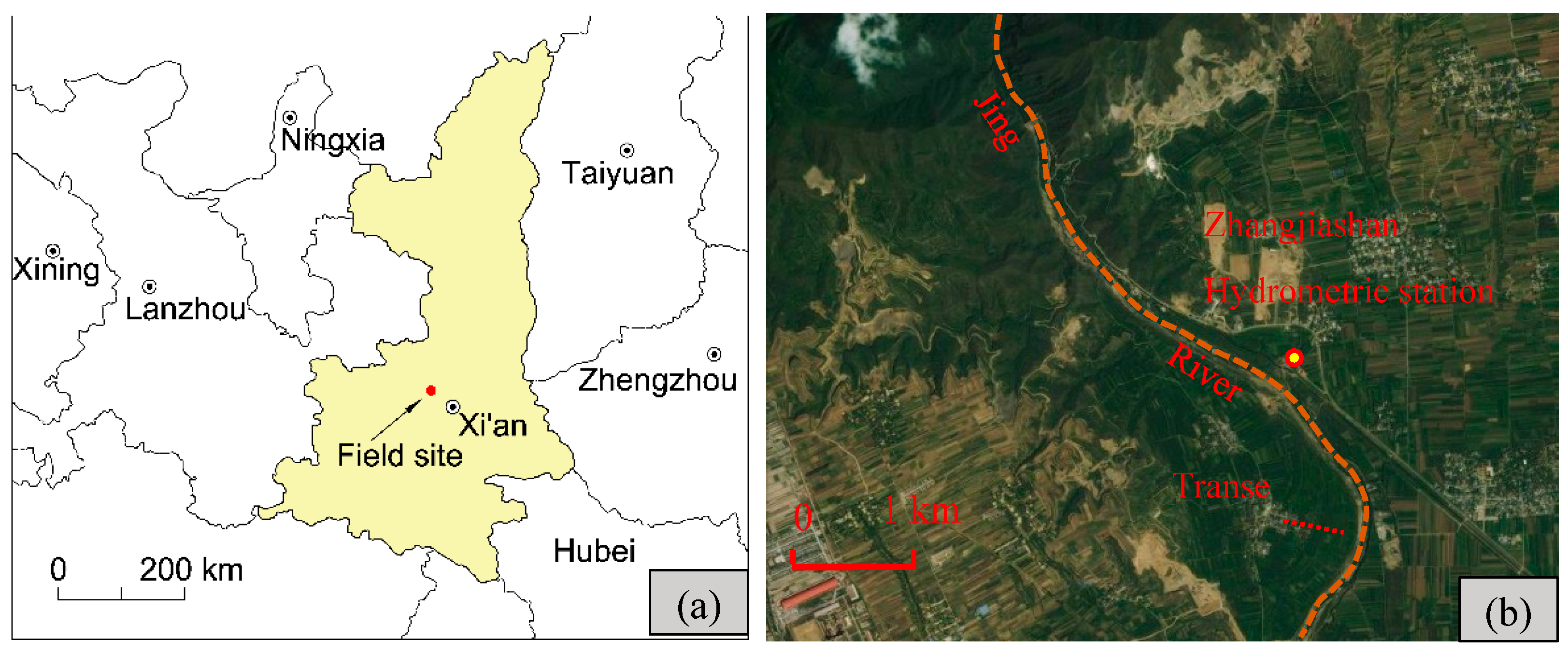
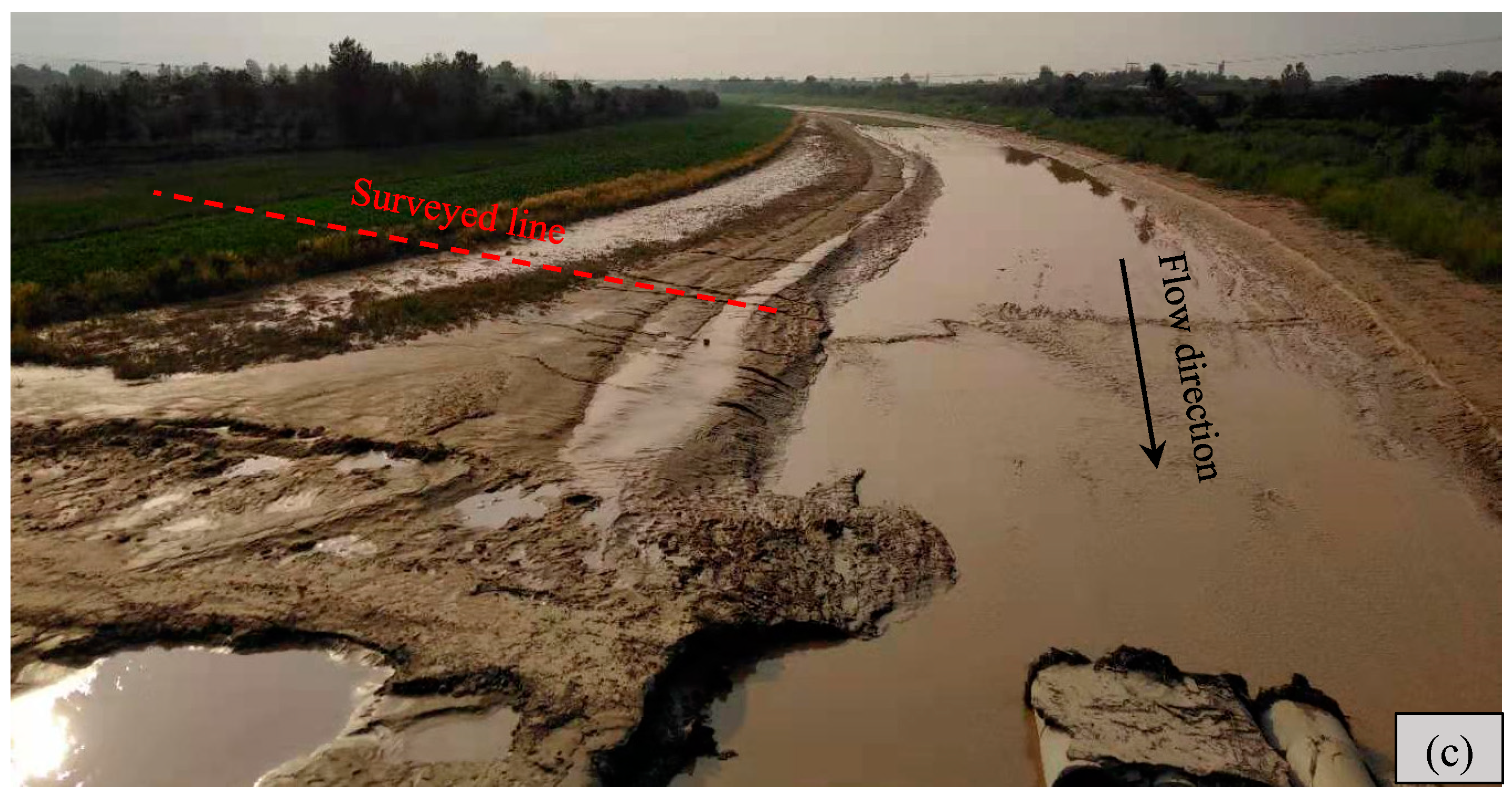
The field site was located at the central Guanzhong Plain of Shaanxi Province (between E 108°34′34″~109°21′35″, N 34°25′20″~34°41′40″), near the Zhangjiashan hydrometric station on the Jing river which is a losing river (discharged to the surrounding aquifer) after a mountain pass (Figure 1). The groundwater table falls continuously due to groundwater over-extraction and a MAR is needed in this agricultural district. The catchment area of Jing River Basin is 45,421 km2, and the average annual runoff is 2.14 billion m3. The maximum peak discharge is more than 9000 m3 s−1, while the minimum dry season discharge is less than 1 m3 s−1, showing the rapidly rising and rapidly falling surface water levels in a hydrological year. Figure 2 depicts the variation of surface water level measured by the Zhangjiashan hydrometric station from 1 January 2006 to 31 December 2014, in which the significant temporal variability of water level with different frequencies can be widely recognized and the amplitude of the fluctuating water level can be 5.3 m above the average water level.
According to the filed investigation, the aquifer of this site is mainly made of loose sands with strong infiltration capacity, a shallow water table, and a high recharge rate. The field transect (Figure 1, about 1.5 km to the Zhangjiashan hydrometric station) is perpendicular to the Jing river, and located at the wash land of Jing river, where the lithology is mainly sandy soil, sandy, and coarse sand. The depth-to-groundwater table along the transect ranges from 2–3 m. A total of 12 slug tests were conducted in simple drillings along the surveyed line at different locations along this transect (Figure 1), and the equation produced by Bouwer and Rice (1989) was used to estimate the hydraulic conductivity. The depth of simple drilling was about 4.00 m at all of the measured locations, and water levels in the drill holes were recorded every second for 30 min using a Solinst level logger. At the site, estimated hydraulic conductivities were in the range of 35 to 46 m d−1. The effective porosity was 0.3, which was measured by a drainage test using the undisturbed soil at this site.
2.2. Conceptual Model and Numerical Model
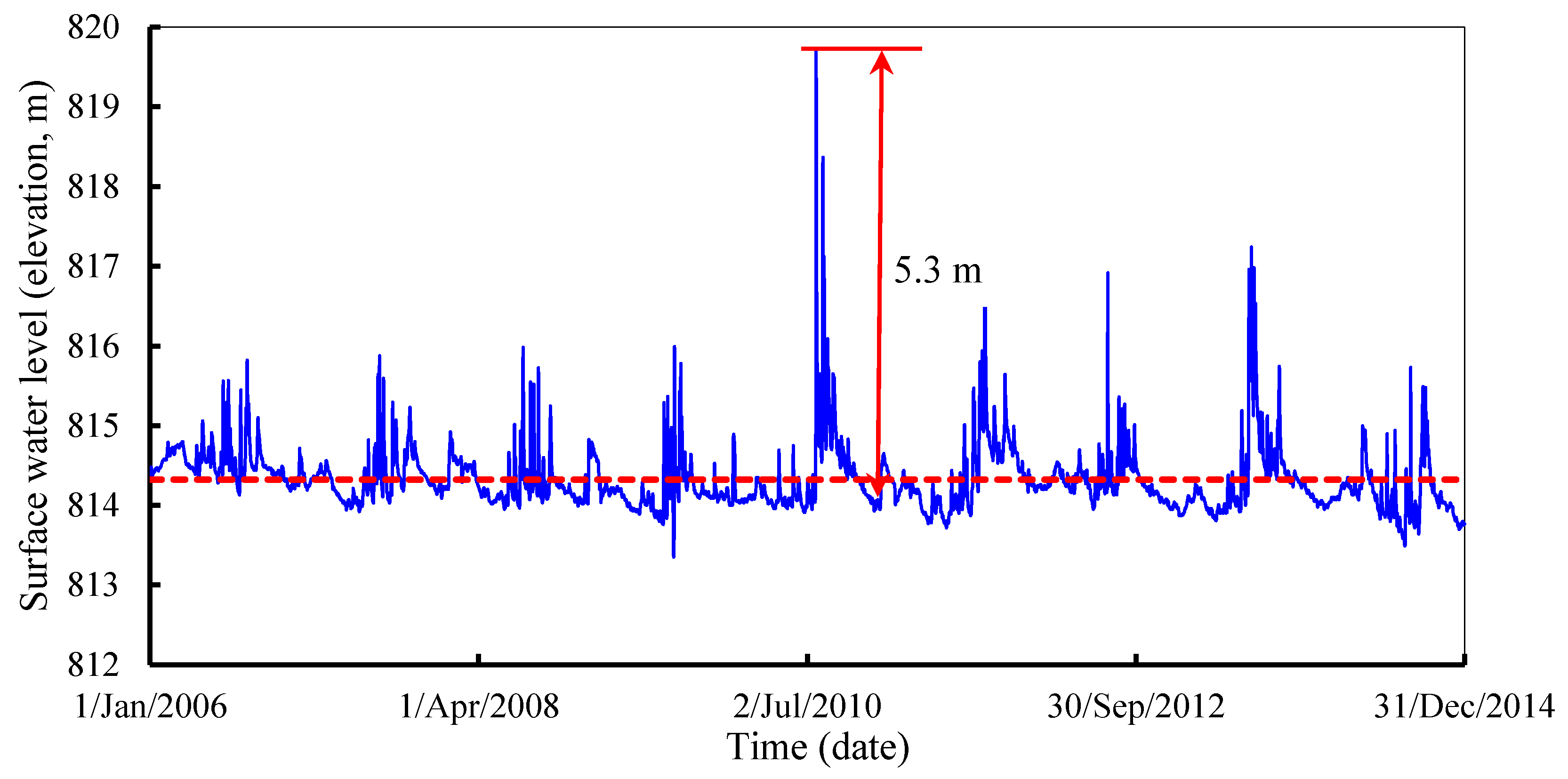
Based on the site investigations, a conceptual model was proposed and the corresponding numerical model based on Feflow [45] was established to simulate variably saturated pore-water flow in an unconfined near-bank aquifer subjected to surface water level fluctuations (Figure 3a). The Richards equation describing the groundwater flow simulated in the Feflow code is shown as below.
where s is the saturation of fluid in the void space [1], is the specific storage coefficient (L−1), h is the hydraulic head (L), t is time (T), is the porosity (void space) [1], is the nabla (vector) operator (L−1), q is the Darcy velocity of fluid (L T−1), Q is the bulk source/sink term of flow (L3 T−1), QEOB is the correction sink/source term of the extended Oberbeck–Boussinesq approximation (T−1), is the relative permeability [1], K is the tensor of hydraulic conductivity [LT−1], is the viscosity relation function [1], is the buoyancy coefficient [1], and e is the gravitational unit vector [1].
The numerical model represented a 2-D vertical section perpendicular to a surface water bank with a length of 500 m and a thickness of 100 m, which assumed groundwater flow was negligible and the GW–SW interaction was uniform, longitudinally to the bank and river direction (Figure 3b). The Dirichlet boundary was applied to the interface of surface water and groundwater representing the surface water level, which varied with time (AF in Figure 3). The slope of the bank was ignored in these simulations. The boundary EF was set as no flux boundaries and the boundary BCD was set as a constant head boundary in this study because of the negligible effects of the variation of surface water and the artificial recharge on this boundary. The upper boundary AB was set as a no flux boundary as the rainfall and evaporation were neglected, so was the bottom boundary DE, which was an impermeable base. A constant flux boundary was applied to the injection well GH, representing a constant flux injection. The parameter values adopted in the numerical model were representative of a typical alluvial fan aquifer formed with cobble and gravel in the Jinghe river basin, in which the hydraulic conductivity was set to 40 m d−1 and porosity was 0.3, according to the site investigations. The unsaturated properties were simulated using the van Genuchten’s equation, as computed in FEflow. The Van Genuchten parameters for all compartments were manually set to α = 4.05 m−1 and n = 1.987 because the grain composition of the sand is similar to that used in Wu et al. [1].
It should be pointed out that we are not intending a recurrence of the groundwater flow in the artificially recharged aquifer driven by the actual surface water level fluctuations in the field site, but to quantify the influences of the period and amplitude of the fluctuating surface water level on the groundwater flow features based on the field investigations. Thus, a sinusoidal fluctuating surface water level [16,46,47] was applied to the boundary AF as the forcing condition in the model, which is shown as below.
where h(t) is the variable surface water level (L) at time t (T); hMSL is the mean surface water level (L); A and ω are the amplitude (L) and frequency (T−1) of the fluctuating water level, respectively.
2.3. Scenarios Definition
Three scenarios (S1, S2, S3) were conducted to investigate the effects of surface water level fluctuations on the performance of a near-bank MAR. The periods and the amplitude of the fluctuating surface water level were justified according to the variation of surface water level at Zhangjiashan hydrometric station. The amplitude of the fluctuating surface water level (A in Equation (3)) varied from 1 to 5m, and the period (2π/ω) varied from 4 to 40 d in S1 and S2, respectively. Only one complete cycle of fluctuations was investigated in this study. The fluctuations of surface water can be divided into two stages, in which the first stage is the surface water level increasing, first to the peak level, then recovering to the average level, and the second stage is the surface water level decreasing first to the trough level and then recovering. Additional simulations were conducted to examine the extent to which the penetration depth of surface water altered the system’s response to fluctuating surface water level conditions in S3, in which the penetration depth of surface water into the aquifer (PDs) was set to 40, 50, 60 and 100 m, respectively. For all simulations performed, the single cycle fluctuating surface water level was applied at the boundary AF, representing the surface water, after the numerical model was initially run to a steady state condition. The numerical model was then run with a stable surface water level (the mean surface water level was 70 m for all simulations) until it returned to a steady state condition.
3. Results
3.1. Groundwater Table
GW table driven by artificial recharge and the fluctuating surface water level in the near-bank aquifer was measured at the observation point (the coordinates of observation point is x = 30 m, z = 60 m) in different scenarios, as shown in Figure 4. Figure 4a shows that the GW table fluctuation in the near-bank aquifer driven by injection is asymmetrical with a larger oscillation above the stable GW table, but smaller below the stable GW table. Expectedly, the recovery of the GW table requires more time than the recovery of the surface water level, and longer periods of surface water level fluctuation lead to a larger oscillation of the GW table, in which the oscillation of surface water level is same. For example, when the fluctuation period was set as 40 d, the amplitude of the GW table at the observation point was 1.43 m above the stable GW table (H = 69.6 m in this scenario) but was much smaller (0.78 m) below that (Figure 4a). It takes over 80 days to recover the groundwater table. As expected, injections in the near-bank aquifer led to an increased GW table. Specifically, Figure 4b shows increased periods of surface water fluctuations leading to smaller increments of peak values in the GW table at observation point H, but larger increments of trough values. The variation law of the peak and trough values of the GW table with the period of surface water level fluctuations could be fitted well by power functions (∆H = αTδ(T), where δ(T) and α are the coefficients) as shown in Figure 4b. Figure 4c shows that increasing surface water penetration depth leads to a decrease in not only the peak values but also the trough values of the GW table. The trend lines of ∆H (increment values of GW table induced by injection) to PDs (penetration depth of surface water) could be fitted by power law relationships (Figure 4c, ∆H = αPDδ(PD), where δ(PD) and α are the coefficients). Furthermore, the effect of the amplitude of the fluctuating surface water level (A) has also been considered in this study, as shown in Figure 4d. The results show the increment of GW table peak values decreases significantly with an increase of the amplitude of the fluctuating surface water level, but the increment of GW table trough values increases slightly with it (indicated by the power exponent, in which the decay exponent of the GW table peak values could be 0.045 but only 0.0117 for GW table trough values). The variation law of the peak and trough values of the GW table with the change of the amplitude of the fluctuating surface water level could be fitted by power functions (∆H = αAδ(A), where δ(A) and α are the coefficients).
If δ is taken as a measure of the effects of different influence factors on water table in this study, the asymmetrical response of GW table to surface water level fluctuations can be quantified. For example, the increment of the GW table trough values increased with the period of the surface water level fluctuation and the increase exponent was 0.0129, but for peak values it was −0.025. The same asymmetrical response of the GW table to the change of A can also be seen in Figure 4d, in which the decay exponent of the increment of GW table peak values could be 0.045, but was only 0.0117 for increments of the GW table trough values. On the contrary, the response of ∆H to the depth that the surface water penetrates to the aquifer seems symmetrical for the decay exponent of the peak values, and the values are almost equivalent (δ(PD) for peak values (−0.594) and for trough values (−0.613).
3.2. Artificially Recharged Water Lens
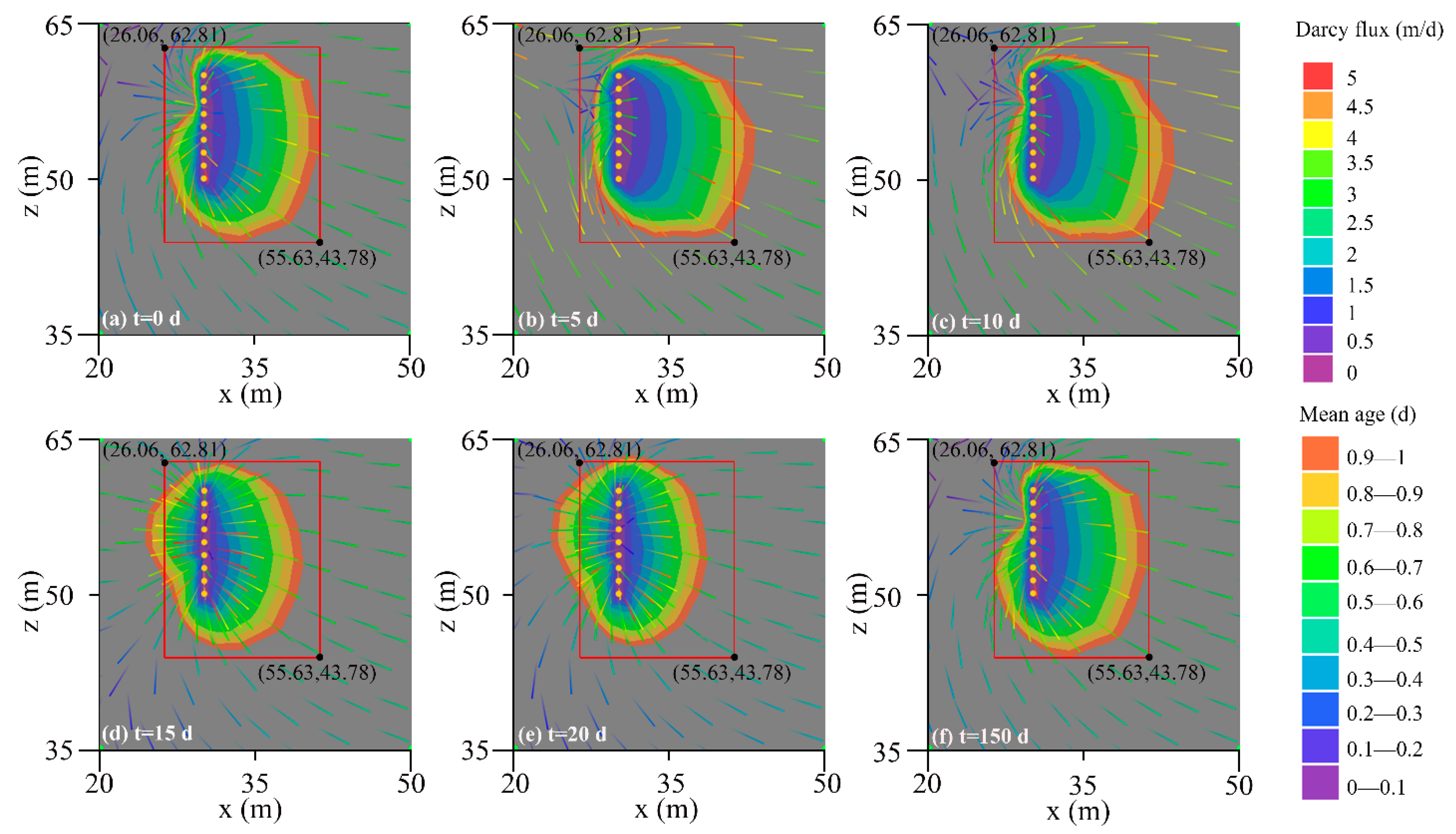
An artificially recharged water lens was formed in artificially recharged areas due to artificially-induced recharge to the lens. Groundwater ages were taken as a natural tracer to visualize the variation of the artificially recharged water lens driven by the fluctuating surface water level in the artificially recharged near-bank aquifer, when the period of surface water fluctuation was set at 20 d and the amplitude was set at A = 5 m (Figure 5). The fringes when maximum groundwater age was 1 day were taken as an example to visualize the artificially recharged water lens. As the surface water level increased, the artificially recharged water lens gradually contracted vertically and extended downward along the regional groundwater flow direction, as compared in Figure 5a,b. This vertical contraction and downward extension continued even when the surface water level recovered after a fluctuation above the average water level, due to the delay in the response of GW table, as shown in Figure 5c. However, the vertical contraction of the lower interface of the ambient groundwater and artificially recharged water is inconspicuous at this time (t = 10 d). From Figure 5d, it can be seen that the artificially recharged water lens extends upward, but contracted downward gradually in response to the decrease in the surface water level, which is more obvious in Figure 5e when the fluctuations of the surface water level had recovered. Furthermore, the artificially recharged water lens contracted in the vertical direction when the surface water level was fluctuating below the average surface water level.
3.3. Groundwater Flow Paths and Travel Times
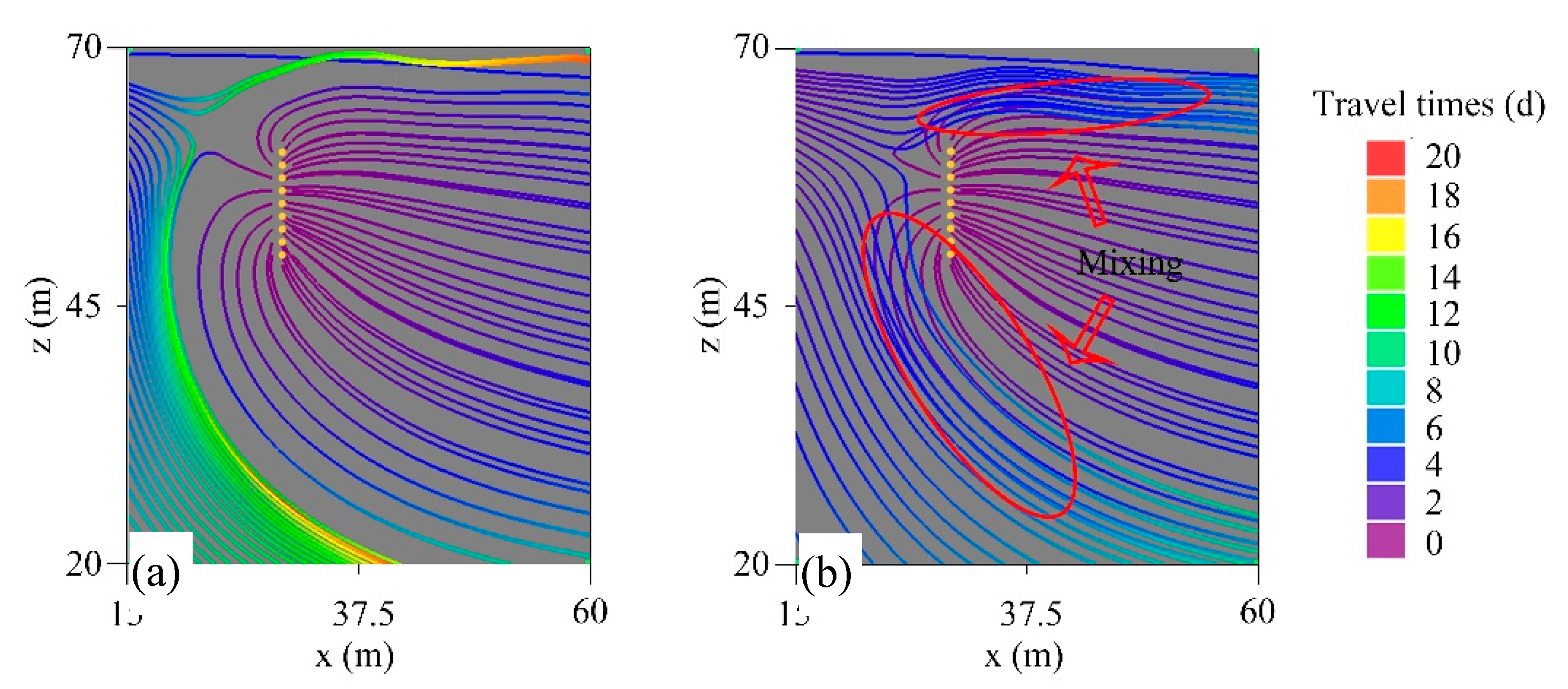
Particle tracking was conducted to examine the flow paths and corresponding travel times of the ambient groundwater (recharged by the fluctuating surface water) and the artificially recharged water driven by the fluctuating surface water level in the managed near-bank aquifer. Particles were released along a vertical line at x = 0 m (tracking the ambient groundwater, or the groundwater that was recharged by the surface water) and along the screen of the injection well (tracking the artificially recharged water, as seen in the yellow nodes in Figure 6). The particles were released at the beginning of the fluctuation of the surface water level, when the flow field was in a steady condition after a long time running from the initial condition. For comparison, the modeling results of particle tracking for the condition with a steady surface water level (HMSL = 70 m, A = 0 m) were also recorded and are shown in Figure 6a. In addition, the modeling results with a fluctuating surface level (HMSL = 70 m, A = 5 m, T = 20 d) are shown in Figure 6b. Figure 6 shows that surface water level fluctuations alter the flow paths of the ambient groundwater and the artificially recharged water significantly. The mixing zone of the ambient groundwater and the artificially recharged water where the flow paths of the ambient groundwater and artificially recharged water cross each other spatially, as induced by the surface water level fluctuations, could be seen in Figure 6b. It should be noted that the cross of the flow paths of the ambient groundwater and the artificially recharged water only occurred spatially, not temporally. That is, the ambient groundwater and artificially recharged water do not flow through the same locations at the same time. Furthermore, Figure 6 also shows that surface water level fluctuations could accelerate the travel times of ambient groundwater significantly but show limited influence on the travel times of artificially recharged water when compared with the steady condition.
The average travel time of artificially recharged water describes the time that water and solutes are exposed to the fluctuating surface water level condition in the artificially managed near-bank aquifer in different scenarios, as provided in Figure 7. The increasing periods of surface water level fluctuations led to an increase in average travel times which could be fitted by a right half branch of a parabola and the R2 could be 0.92, indicating a good performance of the parabola in forecasting the variation law of travel times affected by the change of period of surface water level fluctuations. On the contrary, increasing PD (the depth of river penetration within the aquifer) and A (the amplitude of surface water level fluctuations) would accelerate the artificial water flow and reduce the travel time, which could be fitted by the power functions.
3.4. Discharge of the Near-Bank Aquifer
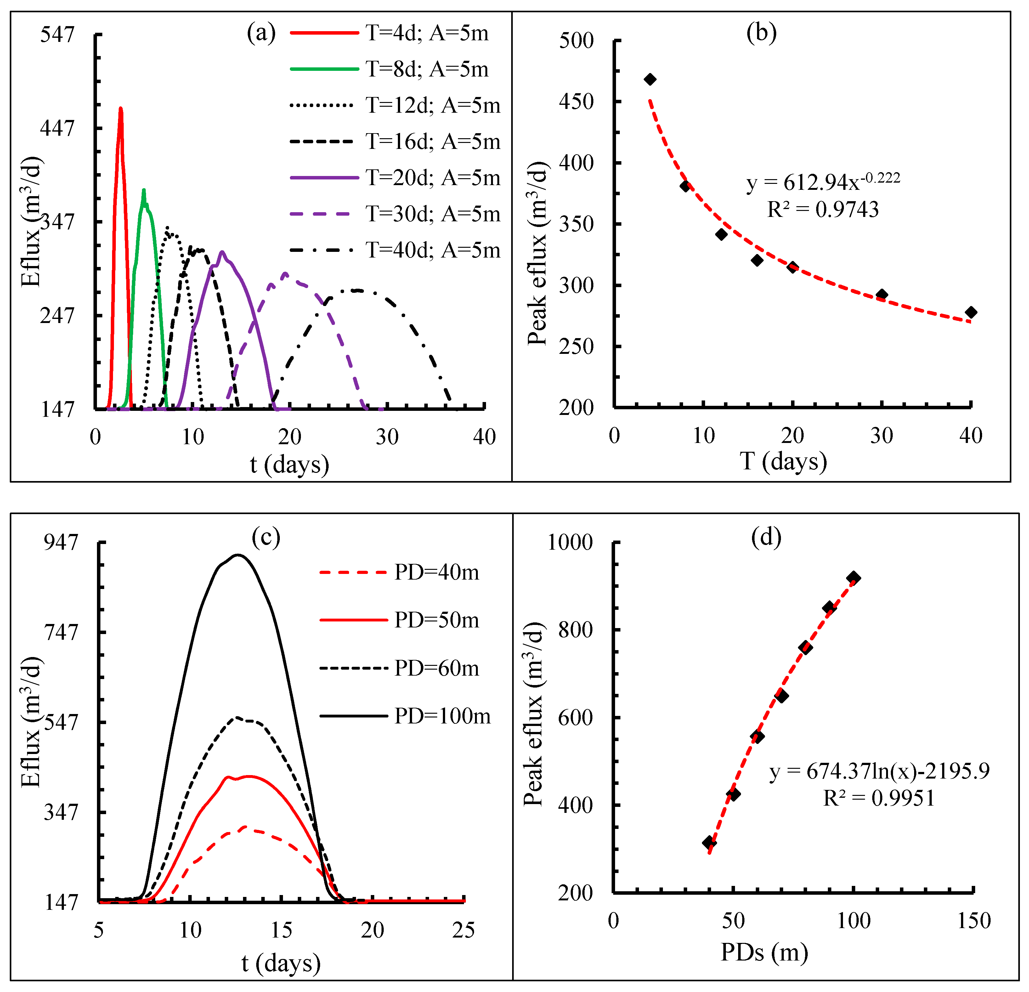
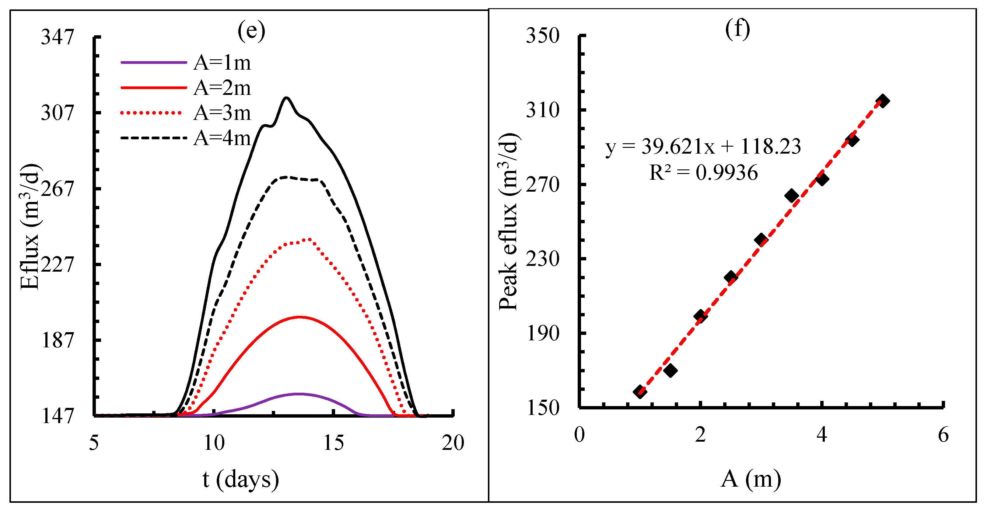
Discharge of the near-bank aquifer was measured at these nodes along the upward boundary (AF). It should be noted that the upward boundary, representing the surface water with fluctuating water level, could be a discharge boundary when the surface water level drops below the groundwater table which is raised by injection. In contrast with the response of the GW table, Figure 8a,c,d show a significant slow discharge response of the near-bank aquifer to surface water level fluctuations, which are delayed with the increasing period of fluctuations (Figure 8a). The fluctuations of near-bank aquifers discharge with times that are totally different with the variation of surface water level, which at first only increase, and then decrease without an increase process after the decrease. Furthermore, according to the results in Figure 8a,b, the longer period of the surface water level fluctuations leads to a smaller peak discharge, which follows a power function. For example, the discharge could be 468 m3 d−1 when the period of surface water level fluctuation is set at 4 d, but only 277 m3 d−1 when the period is 40 d. The discharge induced by surface water level fluctuation increases significantly with the increase of the depth that the surface water penetrates into the aquifer, as, for example, when the discharge of 314 m3 d−1 when the penetration depth of surface water is 40 m in Figure 8c,d, which could be as much as 918 m3 d−1 when the surface water completely penetrates the aquifer. Moreover, the amplitude of the surface water level fluctuations can also lead to an almost linear increase in the discharge of the near-bank aquifer (Figure 8e,f).
4. Discussion
This work examined the influence of fluctuating surface water level on the performance of MAR in a near bank aquifer, which has been largely unexplored so far. In the studied sandy aquifer, previous regional-scale works [14,15,16,17] highlighted that surface water fluctuations may still affect water tables on timescales of hundreds of hours, which has implication on MAR performance. MARs are often conducted in near-bank areas, taking advantage of the low cost associated with the nearby availability of water for artificial recharge, in order to enhance groundwater quantity and reduce seawater intrusion and so on. Here, a numerical model based on a field analog was applied to examine the performance of a MAR subjected to the influence of surface water level fluctuations in a near-bank aquifer. This work assumed a sinusoidal surface water level across a variety of spatial and temporal scales, as a simplification of a complex natural surface water level series, which provided useful insights on the response time and patterns of near-bank aquifers subject to MAR.
Our results showed that the groundwater table is asymmetrical, with a quick rising phase and a slow falling phase consistent with the results reported by Xin et al. [17] and Gerecht et al. [42]. Our numerical simulations showed the same fluctuation amplitude of surface water above and below the average surface water levels leads to an asymmetrically fluctuating groundwater table with larger oscillation above the average groundwater table, but smaller oscillation below it. Because it directly reflects groundwater storage variations, changes in the table elevation are an effective indicator of the performance of MAR. Our results showed that longer period and higher amplitude of surface water level fluctuations lead to larger increments of water table trough values, but smaller increments of peak values, indicating a good performance of MAR because more attention is always paid to the water table trough values. Meanwhile, the limited increment of water table peak values induced by the longer period and higher oscillation of the surface water level fluctuations in the artificially recharged aquifer bears lower risk of the secondary salinization of soil in the near-bank region. The greater depth the surface water penetrates to the aquifer, the smaller the increment of water table peak and trough values, which is not conducive to the performance of MAR. Thus, a MAR is more efficient in near-bank regions where there is a longer period and a higher oscillation of surface water level fluctuation; and the depth to which the surface water penetrates to the aquifer should be smaller.
Near-bank injections can be used to enhance groundwater recharge, but doing so limits the bank filtration processes, which is known to in aid the removal of natural organic matter, pathogenic microbes, and various pollutants from the surface water [48]. Therefore, near-bank injections may lead to a change of groundwater quality because of the differences in the hydro-chemical composition between the surface water and the groundwater. In addition, chemical loading rates have been shown to be strongly controlled by groundwater flow paths and geochemical conditions [28], particularly in arid and semi-arid areas. The alteration of groundwater flow paths by a MAR can lead to changes in the hydro-geochemical characteristics and geochemical processes within specific aquifers [49,50,51]. For these reasons, groundwater flow paths and the variations of the artificially recharged water lens should be considered before the applications of near-bank injections. Our results show that a fluctuating surface water level led to a thinner artificially recharged water lens which was mainly controlled by dynamic groundwater processes similar to the variation of the upper saline plume formed by wave-driven recirculation shown by Xin et al. [31], and this was despite not considering variable fluid density in our study. Furthermore, similar to the results shown by Xin et al. [31], the mixing zones of ambient groundwater and artificially recharged water occurred when the fluctuating boundary representing the surface water was applied to the near-bank aquifer, indicating the geochemical conditions may be altered in these zones. Thus, particular attention should be paid to these zones during the operation of near-bank MAR projects.
The travel time of artificially recharged water from the recharge to the discharge areas determines the rate of many processes occurring in aquifers [52,53]. Shorter travel time might indicate that artificially recharged water has a limit time to improve quality through filtration by a passing aquifer, but longer travel times may reduce the recovery of artificially recharged water. Our results show that longer periods of surface water level fluctuations led to slight increases in the travel times of artificially recharged water, but sharp decreases with the increase of A and PD. This suggests that variations of A and PD are key parameters when considering the operating issues associated with travel times.
Unexpectedly, the fluctuating surface water level curve with a single peak and a single trough led to a single peak discharge curve. This could be attributed to the response of dynamic groundwater pressure fluctuations that is related to the distance to the surface water-groundwater interface. The surface water level fluctuations would be smoothed with the increase of the distance to the bank due to soil damping [17]. Furthermore, the asymmetrical response of the water table, with a larger oscillation above the average water table and a smaller oscillation below that, is another factor leading to the single peak discharge curve. In addition, the upward boundary of the near-bank aquifer can become a discharge boundary when the surface water level fluctuates below the average water level, which can also lead to a single peak discharge curve.
5. Conclusions
MARs are often conducted in near-river regions to enhance groundwater resources, or in near-shore areas to reduce sea water intrusion, where the influences induced by surface water level fluctuations are poorly understood. Based on site investigations in Jinghe river basin, a conceptual model and a corresponding numerical model were conducted to bridge this knowledge gap.
The results of this study indicate an asymmetrical response to surface water level fluctuations of groundwater tables driven by injection. This phenomenon does not just refer to the quick rising groundwater table and slow recovery phase, but includes the asymmetrical amplitudes below and above the stable groundwater table. The response of groundwater table increments values induced by injection to surface water level fluctuation could all be fitted by power functions. That is, the increment of groundwater table peak values decreases with the increase to the period and amplitude of surface water level fluctuation, while the increment of groundwater table trough values increases. Furthermore, the increasing depth to which the surface water penetrates into the aquifer causes smaller incremental changes to groundwater tables induced by injection. In addition, the fluctuating surface water level leads to a thinner artificially recharge water lens.
Mixed zones where the flow paths of ambient groundwater and artificially recharged water cross through the same locations at similar times could be found when the temporally varying surface water level is applied to the artificially recharged near-bank aquifer. The travel times of artificially recharged water increases with an increasing surface water level fluctuation duration, but decrease with an increasing amplitude of fluctuation and the penetration depth of the surface water. The peak discharge flux of the artificially recharged aquifer increases with the increase of the duration and amplitude of fluctuation and the penetration depth of surface water.
Furthermore, because of this study is mainly focused on the numerical simulations, future work using sandbox conditions representative of unstable surface water fluctuations and supported with much more field data should be conducted to widen, and/or challenge, the findings from this research.
Author Contributions
Conceptualization, P.W., J.-C.C.; methodology, P.W.; software, B.C. and S.W.; validation, P.W., L.Z.; formal analysis, P.W.; investigation, P.W. and B.C.; resources, B.C.; data curation, P.W.; writing—original draft preparation, P.W.; writing—review and editing, P.W. and J.-C.C.; visualization, S.W.; supervision, P.W., J.-C.C.; project administration, P.W., L.Z.; funding acquisition, P.W., L.Z. All authors have read and agreed to the published version of the manuscript.
Funding
This research was supported by the National Natural Science Foundation of China (42102286, U1803241, 51779230), the Belt and Road Special Foundation of the State Key Laboratory of Hydrology-Water Resources and Hydraulic Engineering (Nanjing Hydraulic Research Institute. Grant 2020nkms05), the Open Project Program of Key Laboratory of Groundwater Resources and Environment (Jilin University), Ministry of Education (Grant No. 202105002KF), and the Natural Resources Science and Technology Project of Henan Province in 2020 (Henan Natural Resources Han [2020] No. 542-7), providing financial support for the collection of data, their analysis and the writing and publication of the results.
Institutional Review Board Statement
Not applicable.
Informed Consent Statement
Not applicable.
Data Availability Statement
The data used to support the findings of this study are included within the article.
Acknowledgments
The authors acknowledge valuable comments from the reviewers, which led to significant improvement of the paper.
Conflicts of Interest
The authors declare no conflict of interest. We declare that there are no personal circumstances or interests that may be perceived as inappropriately influencing the representation or interpretation of the reported research results.
Abbreviations
| MAR | Managed Aquifer Recharge |
| SWL | Surface Water Level |
| SW | Surface Water |
| WT | Water Table |
| ARWL | Artificially Recharged Water Lens |
| ATT | Average Travel Times |
| PD | Penetration Depth of surface water into the aquifer |
References
- Wu, P.; Shu, L.; Yang, C.; Xu, Y.; Zhang, Y. Simulation of groundwater flow paths under managed abstraction and recharge in an analogous sand-tank phreatic aquifer. Hydrogeol. J. 2019, 27, 3025–3042. [Google Scholar] [CrossRef]
- Liang, X.; Zhan, H.; Zhang, Y. Aquifer Recharge Using a Vadose Zone Infiltration Well. Water Resour. Res. 2018, 54, 8847–8863. [Google Scholar] [CrossRef]
- Schmidt, C.M.; Fisher, A.T.; Racz, A.; Wheat, C.G.; Los Huertos, M.; Lockwood, B. Rapid nutrient load reduction during infiltration of managed aquifer recharge in an agricultural groundwater basin: Pajaro Valley, California. Hydrol. Process. 2012, 26, 2235–2247. [Google Scholar] [CrossRef]
- Bekele, E.; Patterson, B.; Toze, S.; Furness, A.; Higginson, S.; Shackleton, M. Aquifer residence times for recycled water estimated using chemical tracers and the propagation of temperature signals at a managed aquifer recharge site in Australia. Hydrogeol. J. 2014, 22, 1383–1401. [Google Scholar] [CrossRef]
- Dillon, P.; Stuyfzand, P.; Grischek, T.; Lluria, M.; Pyne, R.D.G.; Jain, R.C.; Bear, J.; Schwarz, J.; Wang, W.; Fernandez-Escalante, E.; et al. Sixty years of global progress in managed aquifer recharge. Hydrogeol. J. 2019, 27, 1–30. [Google Scholar] [CrossRef] [Green Version]
- Sprenger, C.; Hartog, N.; Hernandez, M.; Vilanova, E.; Grutzmacher, G.; Scheibler, F.; Hannappe, S. Inventory of managed aquifer recharge sites in Europe: Historical development, current situation and perspectives. Hydrogeol. J. 2017, 25, 1909–1922. [Google Scholar] [CrossRef] [Green Version]
- Lu, C.; Shi, W.; Xin, P.; Wu, J.; Werner, A.D. Replenishing an unconfined coastal aquifer to control seawater intrusion: Injection or infiltration? Water Resour. Res. 2017, 53, 4775–4786. [Google Scholar] [CrossRef]
- Shi, X.; Jiang, S.; Xu, H.; Jiang, F.; He, Z.; Wu, J. The effects of artificial recharge of groundwater on controlling land subsidence and its influence on groundwater quality and aquifer energy storage in Shanghai, China. Environ. Earth Sci. 2016, 75, 195. [Google Scholar] [CrossRef]
- Deng, M. Ground Reservoir: A New Pattern of Groundwater Utilization in Arid North-west China—A Case Study in Tailan River Basin. Procedia Environ. Sci. 2012, 13, 2210–2221. [Google Scholar] [CrossRef] [Green Version]
- Page, D.W.; Peeters, L.; Vanderzalm, J.; Barry, K.; Gonzalez, D. Effect of aquifer storage and recovery (ASR) on recovered stormwater quality variability. Water Res. 2017, 117, 1–8. [Google Scholar] [CrossRef] [PubMed]
- Nicolas, M.; Bour, O.; Selles, A.; Dewandel, B.; Bailly-Comte, V.; Chandra, S.; Ahmed, S.; Marechal, J.C. Managed Aquifer Recharge in fractured crystalline rock aquifers: Impact of horizontal preferential flow on recharge dynamics. J. Hydrol. 2019, 573, 717–732. [Google Scholar] [CrossRef]
- Ghasemizade, M.; Asant, K.O.; Petersen, C.; Kocis, T.; Dahlke, H.E.; Harter, T. An Integrated Approach Toward Sustainability via Groundwater Banking in the Southern Central Valley, California. Water Resour. Res. 2019, 55, 2742–2759. [Google Scholar] [CrossRef]
- Alam, S.; Gebremichael, M.; Li, R.; Dozier, J.; Lettenmaier, D.P. Can Managed Aquifer Recharge mitigate the groundwater overdraft in California’s Central Valley. Water Resour. Res. 2020, 56, e2020WR027244. [Google Scholar] [CrossRef]
- Boano, F.; Harvey, J.W.; Marion, A.; Packman, A.I.; Revelli, R.; Ridolfi, L.; Worman, A. Hyporheic flow and transport processes: Mechanisms, models, and biogeochemical implications. Rev. Geophys. 2014, 52, 603–679. [Google Scholar] [CrossRef]
- Wilson, A.M.; Evans, T.B.; Moore, W.S.; Schutte, C.A.; Joye, S.B. What time scales are important for monitoring tidally influenced submarine groundwater discharge? Insights from a salt marsh. Water Resour. Res. 2015, 51, 4198–4207. [Google Scholar] [CrossRef]
- Sedghi, M.; Zhan, H.B. Hydraulic response of an unconfined-fractured two-aquifer system driven by dual tidal or stream fluctuations. Adv. Water Resour. 2016, 97, 266–278. [Google Scholar] [CrossRef]
- Xin, P.; Wang, S.S.J.; Shen, C.; Zhang, Z.; Lu, C.; Li, L. Predictability and Quantification of Complex Groundwater Table Dynamics Driven by Irregular Surface Water Fluctuations. Water Resour. Res. 2018, 54, 2436–2451. [Google Scholar] [CrossRef]
- Wada, Y.; Beek, L.; Kempen, C. Global depletion of groundwater resources. Geophys. Res. Lett. 2010, 37, 114–122. [Google Scholar] [CrossRef] [Green Version]
- Wada, Y.; van Beek, L.P.H.; Bierkens, M.F.P. Nonsustainable groundwater sustaining irrigation: A global assessment. Water Resour. Res. 2012, 48, 335–344. [Google Scholar] [CrossRef]
- Sawyer, A.H.; David, C.H.; Famiglietti, J.S. Continental patterns of submarine groundwater discharge reveal coastal vulnerabilities. Science 2016, 353, 705–707. [Google Scholar] [CrossRef] [Green Version]
- Barker, J.L.B.; Hassan, M.M.; Sultana, S.; Ahmed, K.M.; Robinson, C.E. Numerical evaluation of community-scale aquifer storage, transfer and recovery technology: A case study from coastal Bangladesh. J. Hydrol. 2016, 540, 861–872. [Google Scholar] [CrossRef]
- Teatini, P.; Comerlati, A.; Carvalho, T.; Gütz, A.-Z.; Affatato, A.; Baradello, L.; Accaino, F.; Nieto, D.; Martelli, G.; Granati, G.; et al. Artificial recharge of the phreatic aquifer in the upper Friuli plain, Italy, by a large infiltration basin. Environ. Earth Sci. 2015, 73, 2579–2593. [Google Scholar] [CrossRef]
- Dashora, Y.; Dillon, P.; Maheshwari, B.; Soni, P.; Davande, S.; Purohit, R.C.; Mittal, H.K. A simple method using farmers’ measurements applied to estimate check dam recharge in Rajasthan, India. Sustain. Water Resour. Manag. 2018, 4, 301–316. [Google Scholar] [CrossRef]
- Li, J.; Chen, J.-J.; Zhan, H.B.; Li, M.G.; Xia, X.-H. Aquifer recharge using a partially penetrating well with clogging-induced permeability reduction. J. Hydrol. 2020, 590, 125391. [Google Scholar] [CrossRef]
- Xia, L.; Zheng, X.L.; Shao, H.B.; Xin, J.; Sun, Z.Y.; Wang, L.Y. Effects of bacterial cells and two types of extracellular polymers on bioclogging of sand columns. J. Hydrol. 2016, 535, 293–300. [Google Scholar] [CrossRef]
- Ward, J.D.; Simmons, C.T.; Dillon, P.J.; Pavelic, P. Integrated assessment of lateral flow, density effects and dispersion in aquifer storage and recovery. J. Hydrol. 2009, 370, 83–99. [Google Scholar] [CrossRef]
- Li, L.; Barry, D.A.; Stagnitti, F.; Parlange, J.Y.; Jeng, D.S. Beach water table fluctuations due to spring-neap tides: Moving boundary effects. Adv. Water Resour. 2000, 23, 817–824. [Google Scholar] [CrossRef]
- Robinson, C.; Xin, P.; Li, L.; Barry, D.A. Groundwater flow and salt transport in a subterranean estuary driven by intensified wave conditions. Water Resour. Res. 2014, 50, 165–181. [Google Scholar] [CrossRef] [Green Version]
- Robinson, C.E.; Xin, P.; Santos, I.R.; Charette, M.A.; Li, L.; Barry, D.A. Groundwater dynamics in subterranean estuaries of coastal unconfined aquifers: Controls on submarine groundwater discharge and chemical inputs to the ocean. Adv. Water Resour. 2018, 115, 315–331. [Google Scholar] [CrossRef]
- Xin, P.; Yuan, L.-R.; Li, L.; Barry, D.A. Tidally driven multiscale pore water flow in a creek-marsh system. Water Resour. Res. 2011, 47, 209–216. [Google Scholar] [CrossRef]
- Xin, P.; Wang SS, J.; Robinson, C.; Li, L.; Wang, Y.G.; Barry, D.A. Memory of past random wave conditions in submarine groundwater discharge. Geophys. Res. Lett. 2014, 41, 2401–2410. [Google Scholar] [CrossRef]
- Malott, S.; O’Carroll, D.M.; Robinson, C.E. Dynamic groundwater flows and geochemistry in a sandy nearshore aquifer over a wave event. Water Resour. Res. 2016, 52, 5248–5264. [Google Scholar] [CrossRef] [Green Version]
- Xiao, K.; Li, H.; Xia, Y.; Yang, J.; Wilson, A.M.; Michael, H.A.; Geng, X.; Smith, E.; Boufadel, M.C.; Yuan, P.; et al. Effects of Tidally Varying Salinity on Groundwater Flow and Solute Transport: Insights From Modelling an Idealized Creek Marsh Aquifer. Water Resour. Res. 2019, 55, 9656–9672. [Google Scholar] [CrossRef]
- Nguyen, T.T.M.; Yu, X.Y.; Pu, L.; Xin, P.; Zhang, C.M.; Barry, D.A.; Li, L. Effects of Temperature on Tidally Influenced Coastal Unconfined Aquifers. Water Resour. Res. 2020, 56, e2019WR026660. [Google Scholar] [CrossRef]
- Yu, X.; Xin, P.; Lu, C. Seawater intrusion and retreat in tidally-affected unconfined aquifers: Laboratory experiments and numerical simulations. Adv. Water Resour. 2019, 132, 103393. [Google Scholar] [CrossRef]
- Geng, X.; Boufadel, M.C.; Rajaram, H.; Cui, F.; Lee, K.; An, C. Numerical Study of Solute Transport in Heterogeneous Beach Aquifers Subjected to Tides. Water Resour. Res. 2020, 56, e2019WR026430. [Google Scholar] [CrossRef]
- Harvey, J.W.; Drummond, J.D.; Martin, R.L.; Mcphillips, L.E.; Packman, A.I.; Jerolmack, D.J.; Stonedahl, S.H.; Aubeneau, A.F.; Sawyer, A.H.; Larsen, L.G.; et al. Hydrogeomorphology of the hyporheic zone: Stream solute and fine particle interactions with a dynamic streambed. J. Geophys. Res. Space Phys. 2012, 117, G00N11. [Google Scholar] [CrossRef] [Green Version]
- Shuai, P.; Cardenas, M.B.; Knappett PS, K.; Bennett, P.C.; Neilson, B.T. Denitrification in the banks of fluctuating rivers: The effects of river stage amplitude, sediment hydraulic conductivity and dispersivity, and ambient groundwater flow. Water Resour. Res. 2017, 53, 7951–7967. [Google Scholar] [CrossRef]
- Ward, A.S.; Schmadel, N.M.; Wondzell, S.M. Time-variable transit time distributions in the hyporheic zone of a headwater mountain stream. Water Resour. Res. 2018, 54, 2017–2036. [Google Scholar] [CrossRef]
- Singh, T.; Gomez-Velez, J.D.; Wu, L.W.; Worman, A.; Hannah, D.M.; Krause, S. Effects of Successive Peak Flow Events on Hyporheic Exchange and Residence Times. Water Resour. Res. 2020, 56, e2020WR027113. [Google Scholar] [CrossRef]
- Inamdar, S.P.; Christopher, S.F.; Mitchell, M.J. Export mechanisms for dissolved organic carbon and nitrate during summer storm events in a glaciated forested catchment in New York, USA. Hydrol. Process. 2004, 18, 2651–2661. [Google Scholar] [CrossRef]
- Gerecht, K.E.; Cardenas, M.B.; Guswa, A.J.; Sawyer, A.H.; Nowinski, J.D.; Swanson, T.E. Dynamics of hyporheic flow and heat transport across a bed-to-bank continuum in a large regulated river. Water Resour. Res. 2011, 47, 104–121. [Google Scholar] [CrossRef]
- Baratelli, F.; Flipo, N.; Moatar, F. Estimation of stream-aquifer exchanges at regional scale using a distributed model: Sensitivity to in-stream water level fluctuations, riverbed elevation and roughness. J. Hydrol. 2016, 542, 686–703. [Google Scholar] [CrossRef]
- Gu, C.; Anderson, W.; Maggi, F. Riparian biogeochemical hot moments induced by stream fluctuations. Water Resour. Res. 2012, 48, W09546. [Google Scholar] [CrossRef] [Green Version]
- Diersch, H. FEFLOW Finite Element Modeling of Flow, Mass and Heat Transport in Porous and Fractured Media; Springer: Berlin/Heidelberg, Germany, 2014. [Google Scholar]
- Fang, Y.; Zheng, T.; Zheng, X.; Yang, H.; Wang, H.; Walther, M. Influence of Tide-Induced Unstable Flow on Seawater Intrusion and Submarine Groundwater Discharge. Water Resour. Res. 2021, 57, e2020WR029038. [Google Scholar] [CrossRef]
- Bakker, M. Analytic Solutions for Tidal Propagation in Multilayer Coastal Aquifers. Water Resour. Res. 2019, 55, 3452–3464. [Google Scholar] [CrossRef]
- Lee, W.; Bresciani, E.; An, S.; Wallis, I.; Post, V.; Lee, S.; Kang, P.K. Spatiotemporal evolution of iron and sulfate concentrations during riverbank filtration: Field observations and reactive transport modeling. J. Contam. Hydrol. 2020, 234, 103697. [Google Scholar] [CrossRef] [PubMed]
- Xing, L.; Guo, H.; Zhan, Y. Groundwater hydrochemical characteristics and processes along flow paths in the North China Plain. J. Asian Earth Sci. 2013, 70–71, 250–264. [Google Scholar] [CrossRef]
- Zhan, Y.; Guo, H.; Wang, Y.; Li, R.; Hou, C.; Shao, J.; Cui, Y. Evolution of groundwater major components in the Hebei Plain: Evidences from 30-year monitoring data. J. Earth Sci. 2014, 25, 563–574. [Google Scholar] [CrossRef]
- Liu, H.Y.; Guo, H.M.; Xing, L.N.; Zhan, Y.H.; Li, F.L.; Shao, J.L.; Niu, H.; Liang, X.; Li, C.Q. Geochemical behaviors of rare earth elements in groundwater along a flow path in the North China Plain. J. Asian Earth Sci. 2016, 117, 33–51. [Google Scholar] [CrossRef]
- Abrams, D. Correcting transit time distributions in coarse MODFLOW-MODPATH models. Ground Water 2012, 51, 474–478. [Google Scholar] [CrossRef] [PubMed]
- Cardenas, M.B. Potential contribution of topography-driven regional groundwater flow to fractal stream chemistry: Residence time distribution analysis of Tóth flow. Geophys. Res. Lett. 2007, 34, 05403. [Google Scholar] [CrossRef]
Figure 1.
(a) Location of the field site near the Jingcun hydrometric station on Jinghe river. (b) Satellite images of the field site. The orange dashed line is the Jiang river and the red dashed line is the surveyed line. (c) Photograph of the field site; the red dashed line is the surveyed line, along which the slug tests were conducted at different locations.


Figure 2.
Variations of water level with time in the Jing river at the Zhangjiashan hydrometric station. The red dashed line is the average value of the surface water level.
Figure 2.
Variations of water level with time in the Jing river at the Zhangjiashan hydrometric station. The red dashed line is the average value of the surface water level.

Figure 3.
(a) Conceptual diagram of the groundwater flows and boundary conditions in an artificially recharged near-bank aquifer exposed to surface water level fluctuations. The PD is the penetration depth of flow path of the artificially recharged water. The surface water penetrates to a depth of PD in the aquifer. TL is the thickness of the artificially recharged water lens. H is the water table. t is the travel time of the artificially recharged groundwater. Parameter h(t) refers to the fluctuating surface water level and the variable head boundary applied to the near-bank aquifer (the red dashed line). The blue dashed line represents the downstream seepage boundary. (b) The subdivision of the model domain. The red line refers to the fluctuating surface water level, which was set as a moving boundary. The blue line refers to the seepage boundary. The yellow line refers to the injection well screen and was set as a flux boundary. H is the observation point.


Figure 4.
GW table and the increment values of peak/trough GW table (∆H) driven by the fluctuating surface water levels and injections at the observation point. (a) the variations of water tables driven by the fluctuating surface table. (b) the variations of ∆H with the change of the period of fluctuations. (c) the variations of ∆H with the change of the penetration depth of SW. (d) the variations of ∆H with the change of the fluctuation amplitude.

Figure 5.
The variation of the artificially recharged water lens is driven by the fluctuating surface water level in the artificially recharged near-bank aquifer. The yellow points are injection nodes, representing the screen of the injection well. (a) is for t = 0 d. (b) is for t = 5 d. (c) is for t = 10 d. (d) is for t = 15 d. (e) if for t = 20 d. (f) is for t = 150 d.

Figure 6.
Simulated flow paths associated with travel times for ambient groundwater particles and artificially recharged water particles through the near-bank aquifer. (a) Scenarios with steady surface water levels. (b) Scenarios with a fluctuating surface water level, in which the T was set as 20 d and A was set as 5 m.

Figure 7.
Simulated average travel times for artificially recharged water through a near-bank aquifer. (a) is the variation of TT with the change of duration of fluctuation. (b) is the variation of TT with the change of penetration depth of SW. (c) the variations of TT with the change of the fluctuation amplitude.

Figure 8.
Discharge of the near-bank aquifer along the AF boundary under the driver of injection and fluctuating surface water levels. Variation of efflux with the change of time under different fluctuation duration, penetration depth of SW and fluctuation amplitude respectively in (a,c,e). Variation of peak efflux with the change of fluctuation duration, penetration depth of SW and fluctuation amplitude respectively in (b,d,f).


Publisher’s Note: MDPI stays neutral with regard to jurisdictional claims in published maps and institutional affiliations. |
© 2021 by the authors. Licensee MDPI, Basel, Switzerland. This article is an open access article distributed under the terms and conditions of the Creative Commons Attribution (CC BY) license (https://creativecommons.org/licenses/by/4.0/).
Share and Cite
MDPI and ACS Style
Wu, P.; Comte, J.-C.; Zhang, L.; Wang, S.; Chang, B. Effect of Surface Water Level Fluctuations on the Performance of Near-Bank Managed Aquifer Recharge from Injection Wells. Water 2021, 13, 3013. https://doi.org/10.3390/w13213013
AMA Style
Wu P, Comte J-C, Zhang L, Wang S, Chang B. Effect of Surface Water Level Fluctuations on the Performance of Near-Bank Managed Aquifer Recharge from Injection Wells. Water. 2021; 13(21):3013. https://doi.org/10.3390/w13213013
Chicago/Turabian StyleWu, Peipeng, Jean-Christophe Comte, Lijuan Zhang, Shuhong Wang, and Bin Chang. 2021. "Effect of Surface Water Level Fluctuations on the Performance of Near-Bank Managed Aquifer Recharge from Injection Wells" Water 13, no. 21: 3013. https://doi.org/10.3390/w13213013
Note that from the first issue of 2016, this journal uses article numbers instead of page numbers. See further details here.