Parsimonious Models of Precipitation Phase Derived from Random Forest Knowledge: Intercomparing Logistic Models, Neural Networks, and Random Forest Models

Abstract

The precipitation phase (PP) affects the hydrologic cycle which in turn affects the climate system. A lower ratio of snow to rain due to climate change affects timing and duration of the stream flow. Thus, more knowledge about the PP occurrence and drivers is necessary and especially important in cities dependent on water coming from glaciers, such as Quito, the capital of Ecuador (2.5 million inhabitants), depending in part on the Antisana glacier. The logistic models (LM) of PP rely only on air temperature and relative humidity to predict PP. However, the processes related to PP are far more complex. The aims of this study were threefold: (i) to compare the performance of random forest (RF) and artificial neural networks (ANN) to derive PP in relation to LM; (ii) to identify the main drivers of PP occurrence using RF; and (iii) to develop LM using meteorological drivers derived from RF. The results show that RF and ANN outperformed LM in predicting PP in 8 out of 10 metrics. RF indicated that temperature, dew point temperature, and specific humidity are more important than wind or radiation for PP occurrence. With these predictors, parsimonious and efficient models were developed showing that data mining may help in understanding complex processes and complements expert knowledge.

1. Introduction

The precipitation phase has a fundamental role in the hydrologic cycle and the energy fluxes between land and atmosphere, which affects the climate system. Due to climate change (CC) and climate warming, the rain to snow ratio is expected to increase, affecting the water supply stored as snowpack for one billion people world-wide in winter as well as affecting large cities in mountainous tropical regions such as the Andes [1]. Additionally, as global temperature raises, the impact on snowpack dynamics and streamflow amount and timing may affect an adequate management of water resources, added to the pressing need of water supply due to urbanization and migration to main cities.

The Andean glaciers are important for fresh water supply, especially in dry arid regions, making them vulnerable to changes in temperature. This happens because the glacier depends on the snow cover to delay mass loss [2]. However, the phase of precipitation is controlled by atmospheric profiles of temperature and moisture [3,4], identified an air temperature increase by approximately 0.1 °C/decade with a tendency to increase in the 1960–1990 period. For this reason, it is necessary to study the driving factors governing the occurrence of the precipitation phase and its variability.

The trend of higher rain to snow ratio under CC affects several aspects of the hydrological functioning of a basin. Furthermore, the phase of the hydrometeors depends on the energy transfer from the atmosphere’s temperature and its water content. Thus, the hydrometeors phases observed at ground stations are influenced by factors such as the vertical profile of temperature, the height of the planetary boundary layer, and the type of temperature gradient [5,6,7]. Changes in precipitation leading to lower snow accumulation decrease the response time of the streamflow and affect the magnitude and the duration of the baseflow in summer. Lower response times of hydrologic basins added to enhanced rainfall extremes due to CC may produce higher frequency of flashfloods with its negative impacts associated. Furthermore, this affects the partitioning of water between evapotranspiration and runoff. Thus, changes in the rain to snow ratio affect the hydrological cycle, the land–atmosphere interaction, and beyond; they have societal impacts from the water management perspective and the assessment of risks related to natural disasters.

Traditionally, air temperature is used to estimate the PP. Empirical relations are calibrated for specific locations [8,9], and are mainly focused on the lower 5% fraction (snow) or values higher than 95% (rain) [10,11]. Other models use a lower and an upper threshold for mixed phase precipitation and then fit a linear or a more complex function to describe the mixed phase range [12,13]. More recently, [11], included humidity content related variables in snow covered mountain regions to model PP, which provided acceptable results. Therefore, the consideration of air moisture related variables provides proxy information about the latent heat fluxes driving energy change in the hydrometeors by sublimation or condensation [14]. Models that consider the hydrometeor temperature (Th) or the dew point temperature (Td) as predictors for PP are grounded in these concepts [15,16].

Few studies investigated the thresholds driving the precipitation phase in the tropical Andes. For instance, [8], compared snow and rain air temperature thresholds between Charquini in Bolivia (ca. 4800 m.a.s.l) and Davos in the Swiss Alps (1590 m.a.s.l). They found differences lower than 0.5 °C, despite its strong humidity and cloudiness seasonality [3,13], with 0% occurrence of snow for temperatures higher than 3–3.5 °C and 100% snow occurrence for temperatures lower than −1–−1.5 °C. Following a classical approach, [17], applied −1 °C and 3 °C thresholds for snow and rain occurrence in the Antisana glacier in Ecuador and fitted a polynomial equation based on the work of [18], to represent the mixed PP. However, the complex orography of the Antisana glacier added to the influence of strong easterly winds, which transport high humidity from the Amazon [4,19], makes this location adequate and scientifically interesting to evaluate the influence of other meteorological variables besides air temperature to derive PP.

The approaches to predict PP change from the variables used for prediction to the type of models used for this purpose. However, due to its simplicity and good performance, logistic models using temperature and/or humidity are of special interest. For instance, [7], used logistic regression models to compute the fraction of snow as a function of various meteorological variables, e.g., air temperature and relative. Their ability to incorporate humidity makes them better to predict the precipitation phase than methods using air temperature alone [11], especially in warm humid sites where the temperature range for solid precipitation increases in relation to dry cool zones [20]. Thus, logistical regression models produced the lowest mean biases compared to observations of snow depth and snow water equivalent [21]. However, despite the relative simplicity to identify the relation of the PP with the predictors in these models, which could make it easier to derive the processes involved, the consideration of more variables is far from straightforward, because expert knowledge is necessary to determine how some processes may be translated into equations. Thus, the use of highly effective data mining models may be an option to study the effect of considering additional variables for PP prediction.

Artificial intelligence (AI) methods have been used successfully in several applications for water resource management [22], where the most widely used approach is utilization of artificial neural networks (ANN). However, due to the simplicity and the highly accurate capabilities in classification and regression problems, random forest (RF) has been explored in water resources more recently. Therefore, in the present study, AI models were used to analyze the complex interacting processes between meteorological variables and PP occurrence. The application of AI methods for PP prediction is a pioneering approach according to the available literature, and the good performance of its application in several fields makes it appealing to evaluate these methods for PP research.

Thus, the aims of the present study were threefold: (i) to evaluate the performance of RF and ANN models in relation to logistic models (LM) to derive PP; (ii) to identify the main drivers of PP occurrence from RF models; and (iii) to use these drivers to develop parsimonious logistic models that can help in understanding the underlying processes in relation to PP occurrence. In Section 2, the study area and the data are described. In Section 3, the methodology is presented. In Section 4, the results are discussed, and in Section 5, the discussion and the concluding remarks are presented.

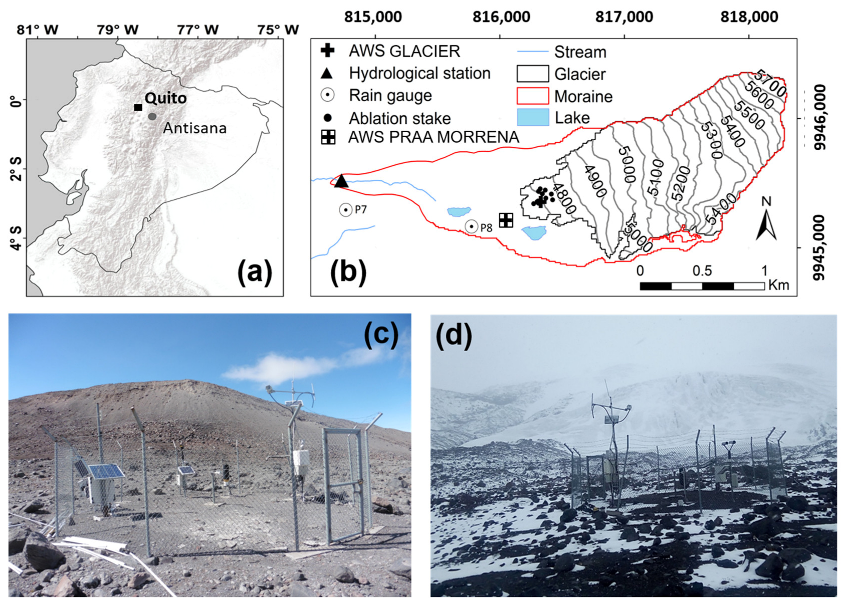
2. Study Area and Data

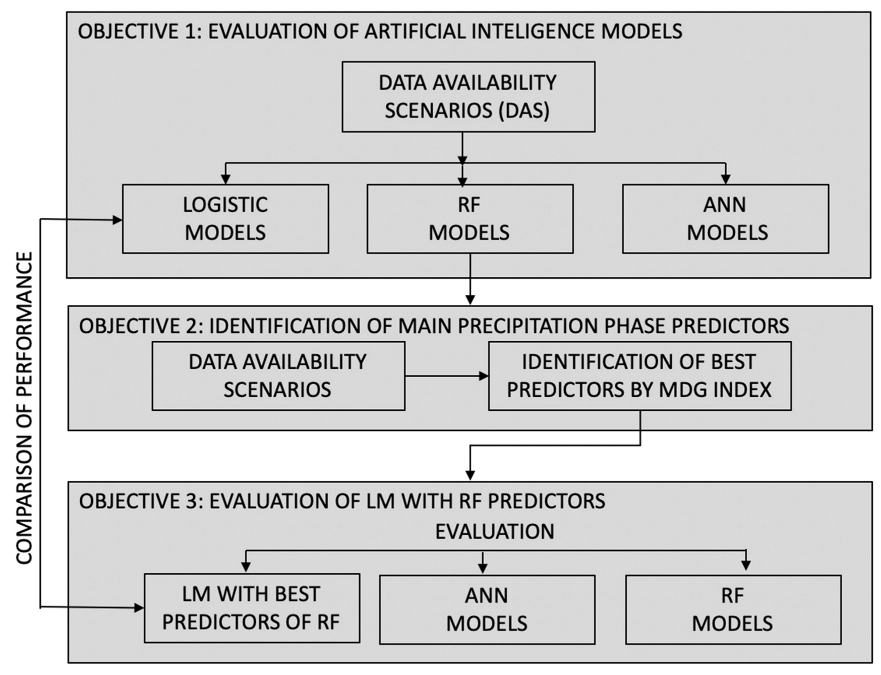
As a part of the Andean Regional Climate Change Adaptation Project/Adaptation to the impact of the accelerated retreat of glaciers in the tropical Andes (PRAA by the acronym in Spanish), the PRAA-Morrena station is in glacier 12 of the Antisana volcano at 4725 m a.s.l, 0°29′38″ S, 78°09′40″ O in the west flank of the Andes Cordillera in Ecuador (Figure 1). Due to its closeness to the glacier, this station is more reliable to study the processes occurring at the terminal zone of the glacier and is more sensitive to changes in temperature and precipitation [23]. In

Table 1. List of sensors installed in the PRAA-Morrena station located in the Antisana glacier 12.

Variable (Unit)	Sensor (Height)	Nominal Accuracy
Air temperature (°C)	Vaisala HPM45AC-shielded (2.00 m)	±0.2 °C
Relative humidity (%)	Vaisala HPM45AC-shielded (2.00 m)	±2% (0–90%)
Wind speed (m ${\mathrm{s}}^{-1}$)	Young 05103 (3.5 m)	±0.3 m${\mathrm{s}}^{-1}$
Wind direction (° deg)	Young 05103 (3.5 m)	±3 deg
Incoming and outgoing SWR (W ${\mathrm{m}}^{-2}$)	Kipp & Zonen CNR4 0.3 < λ < 2.8 µm (1.00 m)	Daily value ±10%
Incoming and outgoing LWR (W ${\mathrm{m}}^{-2}$)	Kipp & Zonen CNR4-G3 5 < λ < 50 µm (1.00 m)	Daily value ±10%

, the sensors installed in this station are presented, and the study site is shown in Figure 1. The meteorological data were sampled every 10 s and recorded every 15 min due to limitations in memory space. The disdrometer OTT Parsivel 2 [24], measures the hydrometeor type and records the cumulative precipitation every 15 min. The disdrometer is located at 4730 m.a.s.l in the glacier foreland of the Antisana volcano.

The disdrometer measured data were corrected [25,26,27,28,29], for diameter, speed, and bulk variables. However, the PP recorded by the disdrometer was considered adequate.

The data were filtered, selecting precipitation higher than 0.1 mm ${\mathrm{h}}^{-1}$, and data with error flags were discarded. Additionally, only data with the meteorological variables available were selected for this study to avoid time series infilling procedure. Finally, 12,248 events were obtained, with 10,747 events between July 2012 and January 2016 for the calibration of models and 1483 observations between July 2019 and February 2020 for the validation.

The dew point temperature, $T_d$, was derived from air temperature, $T_a$ (°C), and relative humidity (RH) using the Magnus equation:

$$T_d=\frac{cr}{\left(b-r\right)} con r=ln\left(RH/100\right)+b{T}_a/\left(c+T_a\right)$$

(1)

where b = 17.67 and c = 243.5 °C [30].

The hydrometeor temperature, $T_h$, may be considered as the ventilated temperature of wet bulb thermometer related to the surface thermodynamic fluxes. Using the approach of [9]:

$$T_h=T_a+\frac{D\left(T_a\right)L\left(T_a\right)}{{\lambda }_t\left(T_a\right)}\left({\rho }_{T_a}-{\rho }_{sat\left(Th\right)}\right)$$

(2)

Due to the non-linear dependence of $T_h$ on both sides of the equation, iteratively, the Newton–Rapson numerical setting was applied [9]. D($T_a$) [${\mathrm{m}}^2 {\mathrm{s}}^{-1}$] is the water vapor diffusion, L($T_a$) [J ${\mathrm{kg}}^{-1}$] sublimation latent heat, ${\lambda }_t\left(T_a\right)$ [J ${\mathrm{m}}^{-1} {\mathrm{s}}^{-1} {\mathrm{K}}^{-1}$] air thermal conductivity, ${\rho }_{T_a}$ [kg ${\mathrm{m}}^{-3}$] water vapor density, and ${\rho }_{sat\left(Th\right)}$ [kg ${\mathrm{m}}^{-3}$] is the saturated water vapor in the surface of the hydrometeor.

The specific humidity was determined by a variation of Equation (17), p. 283 from [31] that uses indirectly T_a and RH:

$$\mathrm{SH}=\frac{e\ast Mvd}{\frac{Patm}{100}} \left[\mathrm{g} {\mathrm{kg}}^{-1}\right]$$

(3)

where Mvd is the ratio between the water vapor molecular weight and the mean molecular weight for dry air.

Here, e is the saturated vapor pressure for moist air given by the next equation:

$$e=\frac{RH}{100}\ast 6.1078 e^{\frac{17.08085\ast Ta}{243.175+Ta}} \left[mb\right]$$

(4)

The list of variables used in the present study is presented in

Table 2. List of variables used in this study.

Variable	Description	Units
Date	Date and hour	Format UTC
Month, hour	Month and hour	Dimensionless
SWRI, SWRR, LWRR, LWRI	Incoming and outgoing SW and LW radiation	$\frac{\mathrm{W}}{{\mathrm{m}}^2}$
$T_a$, $T_h$, $T_d$	Air, hydrometeor, and dew point temperature	°C
RH, SH	Relative and specific humidity	%, g/kg
P	Precipitation	mm
PP	Precipitation phase: 0,0.5,1 for solid, mixed, liquid	Dimensionless

. These variables were used independently or in groups to generate data availability scenarios, as explained below.

3. Methods

The first aim of this study was the evaluation of RF and ANN models to predict PP in relation to LM. In Figure 2, the schematic representation of the methodology is shown. The LMs are simple parsimonious models based on expert knowledge which depend on one or two temperature or humidity related variables, limiting the possibility to evaluate the influence of other variables on PP occurrence. However, RF and ANN models can take several variables as inputs, which may improve the predictive performance of PP. Therefore, data availability scenarios (DAS) were devised to evaluate and compare several LM, RF, and ANN models, which may help to identify the performance of AI models depending on the availability of meteorological data.

For the second aim, the mean decrease Gini index (MDG) was used to identify the main predictors of PP occurrence (see Figure 2). MDG was calculated as the average throughout the forest of the decrease in Gini impurity for a predictor, obeying higher values for the most important variables. Therefore, MDG was used to identify the most important PP weather drivers, which were used to create LMs. These models were created to evaluate the capacity of automatic generation of predictors and compare them with LMs based on expert knowledge. Thus, these models were evaluated against LM, RF, and ANN models from the first objective. A more detailed explanation of the methodology is presented in the following subsections.

3.1. Quality Control of Data

The technical information of the disdrometer used for this study indicated that the accuracies in solid and liquid precipitation were ±5% and ±20%, respectively [24]. In addition, only a few events were classified as solid PP, while high air temperature, e.g., 7 °C, was measured. As such, outliers affected the generation of the liquid phase as well as solid and mixed curves.

Due to the multidimensional nature of the problem, e.g., for each event, in addition to the disdrometer variables, meteorological variables were monitored to classify the large dataset of multidimensional data, and the unsupervised clustering approach k-means was applied. To identify the optimal number of clusters, the silhouette criteria was used. Then, the groups showing physically unfeasible center means (e.g., of PP, air temperature, dew point temperature, and humidity) were removed from the dataset and verified by performing the “S” curve with and without this group. Finally, to furnish the “S” curve [13], temperature bins were selected. For each bin, the median of PP was obtained. This was done for liquid and solid phases. The results obtained using K-means outliers’ detection are shown in Figure 3 ($T_a$, $T_h$, $T_d$ from top to bottom rows). The original data are presented as “S” curves in cyan color, and the black curves were obtained after K-means filtering, which were smoother, as expected [7]. The change produced by this filter was more pronounced for $T_a$ than $T_h$ or $T_d$, as shown in Figure 3.

3.2. Precipitation Phase Forecasting

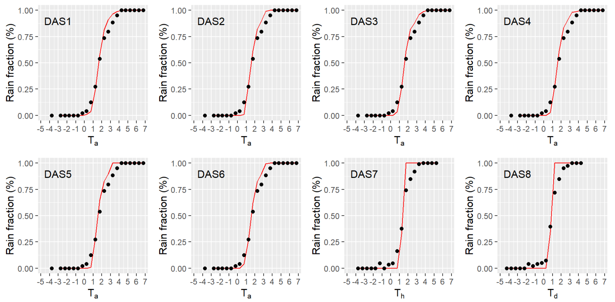
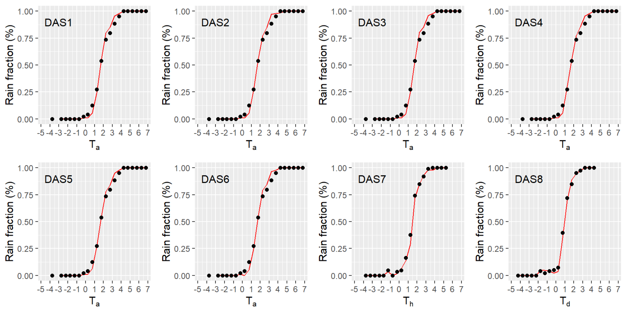
3.2.1. Data Availability Scenarios (DAS)

Despite the data availability of several meteorological variables for this study, 8 data availability scenarios (DAS) were considered. In this fashion, the results may be evaluated depending on the data available to the researcher, helping to evaluate the performance of the models for several DASs. This also indicates the versatility of the models to be applied.

The scenarios are shown in

Table 3. Description of the data availability scenarios (DAS) and the corresponding variables used for each scenario. For all DAS, the target was the precipitation phase.

DAS	SWRI	SWRR	LWRR	LWRI	T	RH	SH	WSPEED	WDIR	T.DewP	T.H
1	X	X	X	X	X	X	X	X	X
2	X	X			X	X
3	X	X	X	X	X	X	X	X	X	X	X
4					X	X	X	X	X	X	X
5					X	X	X
6					X	X
7											X
8										X

. It is worth mentioning that these scenarios were applied only to ANN and RF models, because the LMs are dependent on either $T_a$, $T_h$, or $T_d$. DAS 6 used Ta and RH to compare AI models to LM1. DAS 7 used Th to compare to LM2, and DAS 8 used Td to compare to LM3.

3.2.2. Logistic Models

The PP was considered as a discrete variable, with 0, 1, and 0.5 (dimensionless) for snow, rain, and mixed PP, respectively [10,13]. LMs consider X₁, X₂, … X_n, predictors or independent variables and ${\mathsf{\alpha }}_0, {\mathsf{\alpha }}_1, \dots , {\mathsf{\alpha }}_{\mathrm{n}}$ parameters [32]. In this study, 3 logistic models were evaluated.

Logistic model 1 (LM1) followed the approach proposed by [7]:

$$\mathrm{fr}\left(\mathrm{rain}\right)=\frac{1}{1+{\mathrm{e}}^{\mathsf{\alpha }+{\mathsf{\beta }\mathrm{T}}_{\mathrm{a}}+\mathsf{\gamma }\mathrm{RH}}}$$

(5)

where:

• $\mathrm{fr}\left(\mathrm{rain}\right)$: fraction of rain;
• $\mathsf{\alpha }, \mathsf{\beta }, \mathsf{\gamma }:$ parameters to be calibrated;
• ${\mathrm{T}}_{\mathrm{a}}, \mathrm{RH}:$ air temperature and relative humidity (predictors used in the model).

Logistic models 2 and 3 (LM2) and (LM3) were dependent of the hydrometeor temperature, Th, and the dew point temperature, Td, respectively. Ref. [9], proposed the power logistic equation:

$${\mathrm{f}}_{\mathrm{r}}\left(\mathrm{rain}\right)=\frac{1}{1+{\mathrm{b}}_{\mathrm{x}}\ast {\mathrm{c}}_{\mathrm{x}}{}^{{\mathrm{T}}_{\mathrm{x}}}}$$

(6)

where:

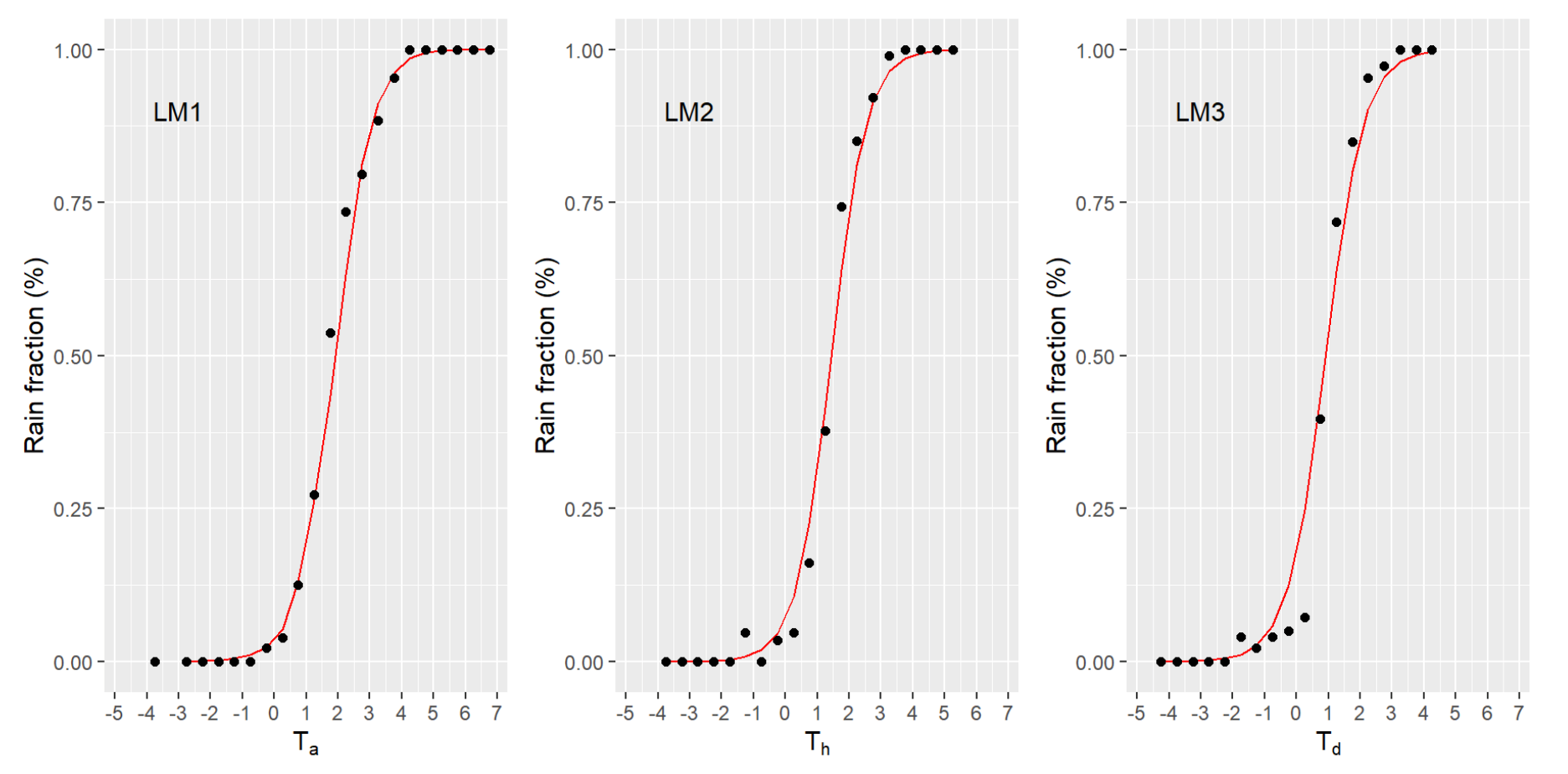
• ${\mathrm{T}}_{\mathrm{x}}:$ is a temperature. For LM2 and LM3, Th and Td were used;
• ${\mathrm{b}}_{\mathrm{x}}, {\mathrm{c}}_{\mathrm{x}}:$ are parameters to be calibrated.

To calculate the precipitation fraction related to a specific temperature, increments of 0.5 °C were used as:

$${\mathrm{f}}_{\mathrm{r}}\left(\mathrm{rain},{\mathrm{T}}_{\mathrm{x}}\right)=\frac{{{\displaystyle \sum }}_{{\mathrm{T}}_{\mathrm{x}}}\mathrm{rain} \left(\mathrm{mm}\right)}{{{\displaystyle \sum }}_{\mathrm{Tx}}\mathrm{Total} \mathrm{precipitation} \left(\mathrm{mm}\right)}$$

(7)

In similar fashion, this equation was applied to solid and mixed precipitation.

To express the LMs as the multiple linear regression (MLR) [33], presented in Equation (8), it was necessary to use the transformation shown in Equation (9). Then, the calibration of parameters for the MLR was conducted.

$$y={\beta }_0+{\beta }_1\ast x_1+\dots +{\beta }_n\ast x_n+\epsilon$$

(8)

$$y=\ln \left(\frac{1-fr}{fr}\right)$$

(9)

Here, y is the dependent variable calculated as Equation (9), $x_i$ represents independent variables, ${\beta }_i$ represents parameters to be calibrated, and $\epsilon$ is a stochastic error. The

Table 4. Multiple linear regression models used for LM.

${\mathit{\beta }}_{\mathit{i}}\ast {\mathit{x}}_{\mathit{i}}$	LM1	LM2	LM3
${\beta }_0$	$\mathsf{\alpha }$	$\ln b_{Th}$	$\ln b_{Td}$
${\beta }_1\ast x_1$	$\mathsf{\beta }\ast T_{air}$	$\ln c_{Th}\ast T_h$	$\ln c_{Td}\ast T_d$
${\beta }_2\ast x_2$	$\mathsf{\gamma }\ast R{H}_{air}$	$-$	$-$

shows the structure of each LM used based on the Equation (9).

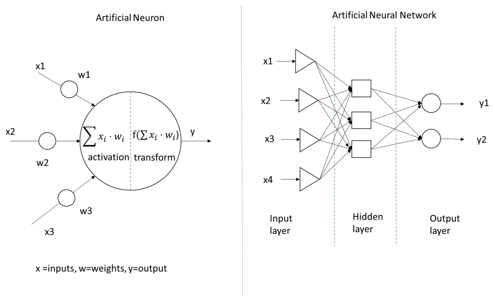
3.2.3. Artificial Neural Networks Models

ANNs are inspired by the functioning of the human brain. They are designed to detect patterns between inputs and outputs by learning algorithms. The artificial neurons have inputs and one output (see Figure 4), and a transfer function transforms the inputs to the output using, as its argument, the weighted sum of inputs. Among the most used transfer functions are the linear, the sigmoid, and the tansigmoid [34].

Artificial neurons are arranged in layers, which are fully connected, and the weights assigned to each connection are defined during the training of the network by complex, highly multidimensional optimization algorithms such as the gradient descent or the Levenberg–Marquart, among others [34]. ANNs are used in classification and regression [35,36]. They are considered as part of the data mining paradigm; therefore, the performance of this approach depends on the data availability. Usually, for calibration, 70% of the data are used, and 30% are used for validation. For a more detailed description of the ANN approach, see [37].

The selection of the transfer functions and the number of neurons for the hidden layer and the output layer was determined iteratively. The tansigmoid transfer function was used in the hidden layer, and the SoftMax function was used in the output layer. These transfer functions are available in the ANN toolbox of MATLAB as part of the “Classification network” option used in this study. For the number of neurons, 3 were used for the output layer and 10 for the hidden layer using the mean square error as loss function. The back-propagation algorithm was used for the optimization of the network synaptic weights. The proportions of data used for calibration, validation, and testing were 70%, 15% and 15%. The data were preprocessed according to the data availability scenarios previously explained, from DAS1 to DAS8. The target vector was one of the following: [0,0,1], [1,0,0], [0,1,0], representing rain, snow, and mixed PP, respectively. For each interval, the rain fraction was calculated as the number of rain events divided by the total events.

3.2.4. Random Forest Models

RF is an AI method based on supervised learning with extensive applications in science and engineering due to its good performance for classification and regression. RF is a group of tools called trees. The forest is formed by a random group of decision trees [38]. Within the forest, every tree is formed by a random sample called bagging, which is the starting point of decision branches. A tree in the end has a decision which counts as a vote, and the decision with the most votes is taken (Figure 5). If more trees are considered, the prediction is more accurate [39].

The RF algorithm may be used to infer discrete or continuous data. Its versatility copes easily with gaps in the data; however, as with any black box model, at the end, the results are shown, but little information is available about the cause of the results [40]. RFs’ ability to cope with forecasting and classification problems makes this technique more attractive for new applications in water resource management. The R library in random forest was used in this study [41]. The reader is referred to the studies of [42] for further information.

3.2.5. Metrics of Evaluation

To evaluate the performances of LM, ANN, and RF models, two kinds of metrics were used, e.g., metrics of detection and metrics of PP fraction quantification, hereafter referred to as fraction quantification metrics. The former measures the detection of snow, rain, or mixed PP events, and the latter measures the fraction of PP for a bin of a variable, for instance, air temperature. The proportions of data for calibration and validation were 80% and 20%, respectively. The data were selected randomly to avoid any trend, which also improved the robustness of the models.

Metrics of Fraction Quantification

The observed and the simulated precipitation phases are represented as Xobs(i) and Xsim(i), and the corresponding fractions are fr_obs(k) and fr_sim(k). N is considered as the number of observations, and M is the number of bins for the representation of a variable.

The mean bias, MB, indicates positive or negative departure from the observed data. Thus, a value of 0 indicates a null difference of means. The MB is calculated as:

$$MB=\frac{1}{M}{\displaystyle \sum }_{k=1}^M\left(f{r}_{sim}\left(k\right)-f{r}_{obs}\left(k\right)\right)$$

(10)

The RMSE of the precipitation fraction was calculated as:

$$RMSE=\sqrt{\frac{{{\displaystyle \sum }}_{k=1}^M{\left(f{r}_{sim}\left(k\right)-f{r}_{obs}\left(k\right)\right)}^2}{M}}$$

(11)

The explained variance of the precipitation fraction was calculated as:

$$r^2=\frac{{{\displaystyle \sum }}_{k=1}^M\left[\left(f{r}_{obs}\left(k\right)-\overline{f{r}_{obs}}\right)\ast \left(f{r}_{sim}\left(k\right)-\overline{f{r}_{sim}}\right)\right]}{\sqrt{{{\displaystyle \sum }}_{k=1}^M{\left(f{r}_{obs}\left(k\right)-\overline{f{r}_{obs}}\right)}^2\ast {{\displaystyle \sum }}_{k=1}^M{\left(f{r}_{sim}\left(k\right)-\overline{f{r}_{sim}}\right)}^2}}$$

(12)

The Nash–Sutcliffe index (NSE) evaluates the representation of extreme values. NSE values of 1, 0, and negative are related to the best model, a model as the mean value, and a model inferior in prediction to the mean value [43]. NSE was calculated as:

$$NSE=1-\frac{{{\displaystyle \sum }}_{k=1}^M{\left(f{r}_{sim}\left(k\right)-f{r}_{obs}\left(k\right)\right)}^2}{{{\displaystyle \sum }}_{k=1}^M{\left(f{r}_{obs}\left(k\right)-\overline{f{r}_{obs}}\right)}^2}$$

(13)

The Kling–Gupta coefficient (KGE) was used to overcome some limitation of the NSE. The best model has a value of 1, and some authors argue that positive values are generally good models and negative values are bad models, although others argue that values less than 0, e.g., −0.41 [43], indicate the benchmark comparison with the mean. The KGE was calculated as:

$$KGE=1-\sqrt{{\left(r-1\right)}^2+{\left(\frac{{\sigma }_{{fr}_{sim}}}{{\sigma }_{{fr}_{obs}}}-1\right)}^2+{\left(\frac{\overline{f{r}_{sim}}}{\overline{f{r}_{obs}}}-1\right)}^2}$$

(14)

where:

• ${\sigma }_{{fr}_{sim}}$ and ${\sigma }_{{fr}_{obs}}$ are the standard deviation of the simulated and the observed fractions.
• $r$ is the linear correlation.

Metrics of Detection

To evaluate the misclassified events (PM) and the unclassified events (PU), the indexes PM and PU were calculated as shown in the paragraphs below. Events with fractions between 5% and 95% were considered as unclassified, whereas a misclassification was considered if the model simulated below 5% (snow) and rain was observed, or if the model simulated a PP fraction over 95% (the rain) and snow was observed. Following [7], to minimize uncertainties related to the phase of precipitation, the mix precipitation values were excluded.

$$PM=\frac{{{\displaystyle \sum }}_{i=1}^{N}Misclassified events \left(X_i,Y_i\right)}{N}$$

(15)

$$PU=\frac{{{\displaystyle \sum }}_{i=1}^{N}Unclassified events \left(X_i,Y_i\right)}{N}$$

(16)

The critical success index (CSI) is the ratio of the correct forecast to the sum of the correct forecast, plus false alarms, plus misses. The perfect model has a value of 1.

$$CSI=\frac{{{\displaystyle \sum }}_{i=1}^{N}Rain cases \left(X_i\cap Y_i\right)}{N-{{\displaystyle \sum }}_{i=1}^{N}Snow cases \left(X_i\cap Y_i\right)}$$

(17)

The snowfall change (SFC) and the precipitation accumulative error (PAE) measured the cumulative error in snow to rain ratio [10]. As mentioned, mixed events were excluded.

$$SFC=\frac{S_{cal}-S_{obs}}{S_{obs}} \left(9\right)$$

(18)

$$Rain Error=\frac{\sum S_{cal}\left(i\right)-S_{obs}\left(i\right)}{Preci{p}_{rain+snow}} for S_{obs}\left(i\right)<S_{cal}\left(i\right)$$

(19)

$$Snow Error=\frac{\sum S_{obs}\left(i\right)-S_{cal}\left(i\right)}{Preci{p}_{rain+snow}} for S_{obs}\left(i\right)>S_{cal}\left(i\right)$$

(20)

$$PAE=Rain Error+Snow error$$

(21)

where:

• $S_{obs}\left(i\right)$ and $S_{sim}\left(i\right)$ are the observed and the simulated snow indicators.

Normalization of Metrics

To ease the interpretation of the results, a normalization process was applied to all models’ evaluation metrics. All metrics were mapped to the range 0 to 1, with a value of 0 for the best model and 1 for the worst model. It is important to clarify that, with metrics such as r² where 1 is the best value, the transformation 1–r² was applied.

For other metrics, the normalization was achieved by simply dividing the metric for a model $x_i$ by the maximum value among all models, as follows:

$$N\_x_i=\frac{x_i}{\max {\left(x\right)}_{all}}$$

(22)

where:

• $N\_x_i$ is the normalized value of a x metric for a model i.

In

Table 5. Description of evaluation metrics and normalized counterparts.

Metric	Range and Interpretation	Metric	Range and Interpretation
r2	max 1 is a perfect model	N_r2	[0–1]: 0 is the best model
kge	max 1 is a perfect model	N_kge	[0–1]: 0 is the best model
rmse	value of 0 is perfect model	N_rmse	[0–1]: 0 is the best model
nash	max 1 is a perfect model	N_nash	[0–1]: 0 is the best model
bias	value of 0 is perfect model	N_bias	[0–1]: 0 is the best model
CSI	max 1 is a perfect model	N_CSI	[0–1]: 0 is the best model
PU	value of 0 is perfect model	N_PU	[0–1]: 0 is the best model
PM	value of 0 is perfect model	N_PM	[0–1]: 0 is the best model
SFC	value of 0 is perfect model	N_SFC	[0–1]: 0 is the best model
PDA	value of 0 is perfect model	N_PDA	[0–1]: 0 is the best model

, the description of the metrics together with the normalized description are shown.

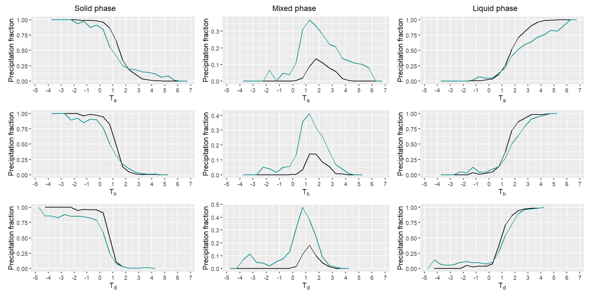
3.3. Meteorological Drivers

An important step towards the development of a model is the identification of predictors. Despite the higher performance of AI models over LM, a pitfall is the lack of information about the processes being modeled and the interrelation between predictors and targets. The principal aim of this section was to evaluate the main meteorological drivers for each DAS. Once these main predictors were determined, simpler models, e.g., LM, were developed, as discussed in the next section. This approach might help to understand complex processes unveiling the interrelation of predictors and targets using “automatic methods” or algorithms.

The evaluation of the importance of variables in RF can be achieved using two indexes, e.g., the mean decrease Gini (MDG) and the mean decrease accuracy (MDA) [39]. Authors such as [44], concluded that the ranking stability of MDG was superior to MDA for data without correlation between parameters. The main reason for this affirmation is that MDA measures may be scaled by dividing by its empirical standard error. However, MDG has shown to be sensitive to predictors with different scales of measurement, and MDG may be preferred over MDA because of increased stability [45]. Thus, MDG was used in this study to identify the main predictor for RF models in all DAS.

3.4. Development of LM Models from the Knowledge of Artificial Intelligence Models

Once the best predictors derived from RF using MDG were determined, logistic models were implemented and evaluated. This step was important because the logistic models use expert knowledge, whereas, here, we proposed to use AI derived knowledge to implement conceptual models.

Thus, after the evaluation of the best predictors for each DAS using the MDG index, LM type models were devised as:

$$fr\left(rain\right)=\frac{1}{1+e^{{\mathsf{\alpha }}_{LM}+{\mathsf{\beta }}_{LM}\ast x_1+{\mathsf{\gamma }}_{LM}\ast x_2}}$$

(23)

where:

• fr(rain) is the fraction of rain;
• ${\mathsf{\alpha }}_{LM}$, ${\mathsf{\beta }}_{LM}$, ${\mathsf{\gamma }}_{LM}$ are parameters to be calibrated;
• x₁ and x₂ are independent variables extracted from MDG.

4. Results

4.1. Evaluation of Artificial Intelligence Methods for Precipitation Phase Forecasting

4.1.1. Logistic Models

In

Table 6. Results of the calibration for logistic models.

Model	LM1			LM2		LM3
Parameter	α	Β	γ	bh	ch	bd	cd
Min	−11.02	−1.67	0.02	12.26	0.15	4.38	0.17
P50	−4.65	−1.63	0.08	13.88	0.16	4.62	0.19
Max	0.96	−1.57	0.14	15.88	0.17	5.09	0.2

, the calibrated parameters for LM1 to LM3 are shown, in addition to the range used for its calibration.

As shown in Figure 6, from left to right, the performance of LM1 was superior to LM2 and LM3 and had a better fit, especially for lower and upper values of PP. Considering that LM1 considered relative humidity in addition to temperature, this result is in concordance with the study of [46], who reported that discrimination of PP at ground level was more accurate considering air saturation parameters in addition to temperature parameters.

A higher influence of Th for the processes related to PP was evident from its better performance to predict PP in comparison to Td, which showed shortcomings, especially in values between −1 °C and 1 °C PP. However, both models LM2 and LM3 slightly underestimated higher values of PP and overestimated the lower values of PP. Further evaluation is needed in relation to the discrimination thresholds of percentiles 5 and 95 to separate solid from liquid precipitation. Such an analysis will be conducted in future research. Such an analysis is important to compare the thresholds determined in other latitudes, as in as Bolivia by [8].

4.1.2. ANN Models

In Figure 7, the results of rain fraction for the eight DASs are presented. The simulation of DAS1 to DAS6 was good, but for DAS7 and DAS8, ANN models overestimated the high values of PP. For mixed PP, DAS1 to DAS6 were well represented with the observed percentile of 50. This fact shows that ANN models captured intermediate PP better than LM1 and LM2. For low PP, ANN models showed clear shortcomings, underestimating PP for all DASs. This is a clear limitation of this approach because it was present for all DASs, regardless of the predictor variables used in the models.

As mentioned in Section 3.2.1, DAS6, DAS7, andDAS8 were devised to compared AI models to LM1, LM2, and LM3. The results of Figure 7 show that more variables such as DAS1 helped to improve PP representation, but the results for DAS6 surpassing DAS7 and DAS8 agree with the results obtained for LM1, LM2, and LM3. Thus, in addition to temperature related variables, the use of humidity related variables showed better results, regardless of the model.

4.1.3. Random Forest Models

The representation of rain fraction for RF is shown in Figure 8. For high PP values, RF captured well the observed data. The PP under 50% was captured adequately for all DASs. The higher and the lower PP values were well represented, clearly outperforming ANN and LM models. The comparison between DAS6, DAS7, and DAS8, did not show a significant difference, as was evident for LM and ANN models. Thus, the importance of variables using the RF approach may be more adequate using MDG, as discussed in the next section.

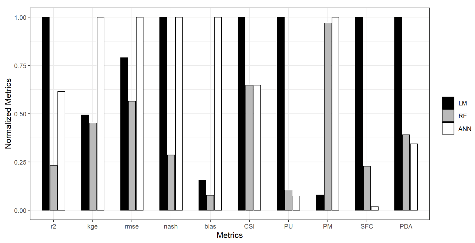
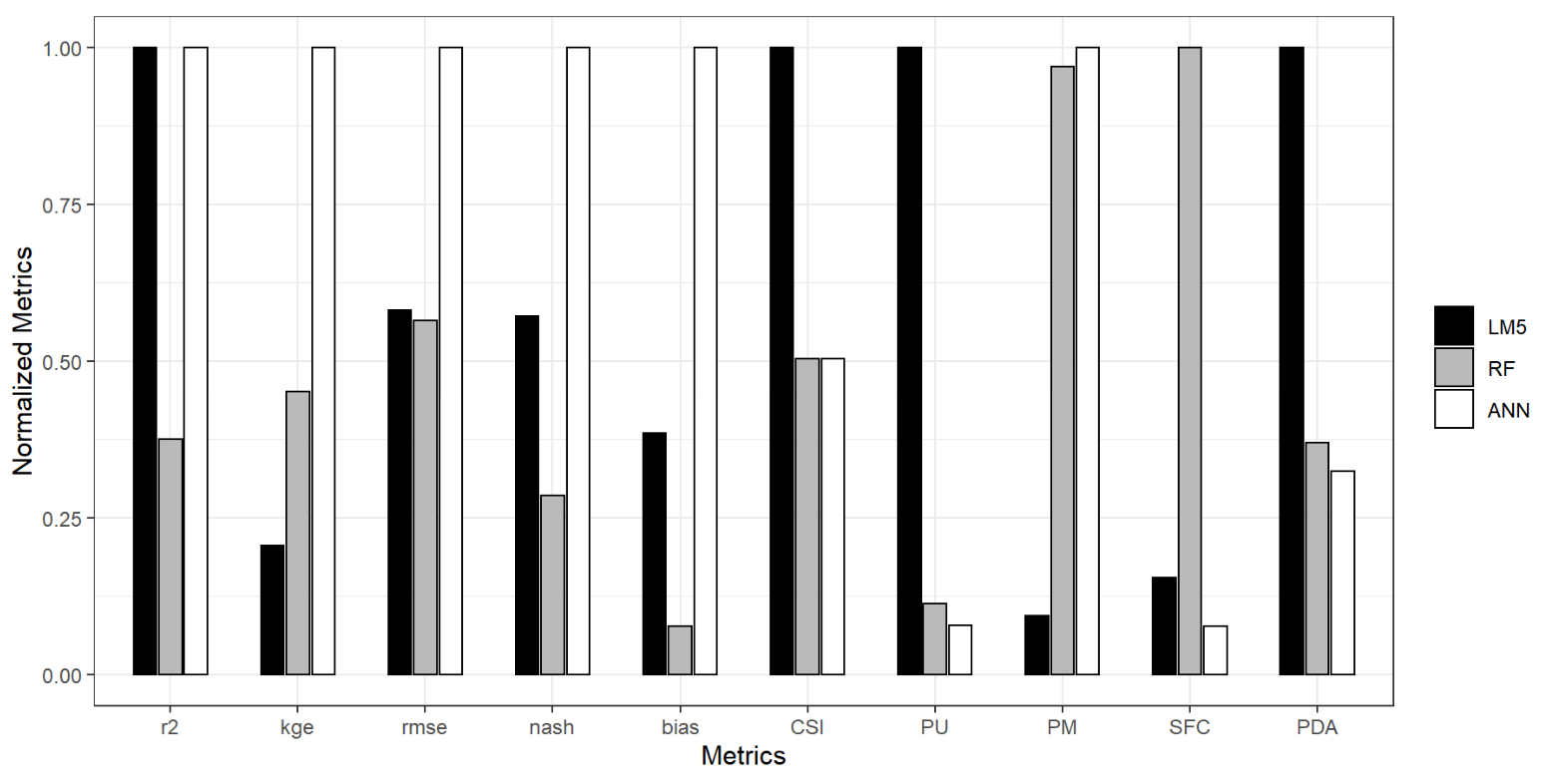
4.1.4. Intercomparison of LM, ANN, and RF Models

For further analysis and models intercomparison, in this section, several metrics of fraction quantification and detection are calculated. In Table 5, the fraction quantification metrics are in lower case, e.g., r₂, kge, rmse, nash, and bias, whereas the detection metrics are in upper case, e.g., CSI, PU, PM, SFC, and PAE.

LMs showed similar results for quantification and detection metrics. However, LM1 metrics corresponded to the visual appreciation of Figure 6, showing it was better at simulating extremes than LM2 and LM3 according to kge. Due to the slight differences among models, the last column in

Table 7. Metrics for LM, ANN, and RF models. Fraction quantification and detection metrics are in lowercase and uppercase, respectively.

MODEL	r2	kge	rmse	nash	bias	CSI	PU	PM	SFC	PDA	Score
LM 1	0.989	0.979	0.043	0.989	−0.008	0.74	0.68	0.008	−0.005	255.655	4
LM 2	0.992	0.965	0.041	0.991	−0.003	0.841	0.729	0.003	−0.046	212.131	2
LM 3	0.981	0.948	0.063	0.979	0.004	0.868	0.807	0.003	−0.121	220.246	4
RF_1	0.997	0.963	0.035	0.996	0.002	0.905	0.07	0.049	0.017	70.4	1
RF_2	0.997	0.964	0.035	0.996	0.002	0.895	0.072	0.055	0.023	77.8	1
RF_3	0.997	0.962	0.037	0.996	0.003	0.903	0.069	0.05	0.016	71.1	0
RF_4	0.998	0.963	0.035	0.996	0.006	0.891	0.068	0.057	0.01	78.5	2
RF_5	0.998	0.967	0.032	0.997	0.004	0.886	0.074	0.059	0.012	84.9	2
RF_6	0.998	0.965	0.034	0.996	0.004	0.888	0.073	0.058	0.01	83.2	1
RF_7	0.997	0.98	0.033	0.997	−0.007	0.83	0.099	0.088	0.014	134.4	5
RF_8	0.996	0.976	0.042	0.995	−0.004	0.849	0.091	0.078	−0.001	117.9	1
ANN_1	0.995	0.942	0.05	0.991	0.012	0.898	0.059	0.054	0.007	69.3	3
ANN_2	0.995	0.936	0.054	0.99	0.013	0.891	0.055	0.058	0.005	72.2	1
ANN_3	0.995	0.947	0.048	0.992	0.012	0.9	0.059	0.053	−0.002	68.3	5
ANN_4	0.994	0.934	0.055	0.989	0.015	0.885	0.052	0.062	0.002	74.8	1
ANN_5	0.994	0.932	0.058	0.989	0.015	0.879	0.052	0.065	0	79	1
ANN_6	0.995	0.935	0.054	0.99	0.015	0.882	0.052	0.063	0.001	76.6	2
ANN_7	0.987	0.9	0.087	0.975	0.01	0.842	0.052	0.087	−0.001	104.8	2
ANN_8	0.985	0.89	0.092	0.971	0.014	0.87	0.052	0.07	−0.005	85	1
MEAN VALUES
LM	0.987	0.964	0.049	0.986	−0.002	0.816	0.738	0.005	−0.057	229.344	2
RF	0.997	0.967	0.035	0.996	0.001	0.881	0.077	0.062	0.013	89.775	5
ANN	0.992	0.927	0.062	0.986	0.013	0.881	0.054	0.064	0.001	78.75	4

shows a score calculated as the sum of the best of the group, 1, or 0 otherwise. Thus, models LM1 and LM3 showed better performance than LM2.

ANN models showed that NSE was less sensitive to kge among models. Thus, based on the kge index, ANN models for DAS1 and DAS3 performed slightly better than the rest of the models. RF models in all DASs showed similar results on quantification metrics, with DAS7 and DAS8 having a better fit on extreme values. However, DAS1 and DAS3 had better results in detection metrics. The scores showed that RF for DAS7 was the best RF model in five out of 10 metrics, followed by DAS4 and DAS5. Again, despite the good performance of RF models, it was difficult to easily interpret the reasons why a DAS showed better results. The results of the mean values (Table 7) showed that, overall, RF models had a better performance than ANN models and that LMs were less skillful than both AI models. Thus, RF models showed a robust performance for modeling PP in relation to LM and ANN.

The normalized metrics are displayed in Figure 9. The good performance of RF models was evident for fraction quantification metrics, where five out of five results were the best models, followed by LM and ANN. For detection metrics, ANN models showed a better performance than RF, and LMs were less skillful than ANN and RF. Based on these results, added to the analysis of the results of Table 7, overall, AI models performed better than LM, and RF showed better results than ANN models.

The superiority of AI models over LM was expected, firstly because of their ability to map several input variables to represent an output and secondly because of the power of machine learning algorithms. However, an interesting result is the superiority of RF over ANN models. This may be related to the fact that detection of rain, snow, or mixed PP is a classification problem, where discrete outcomes are expected.

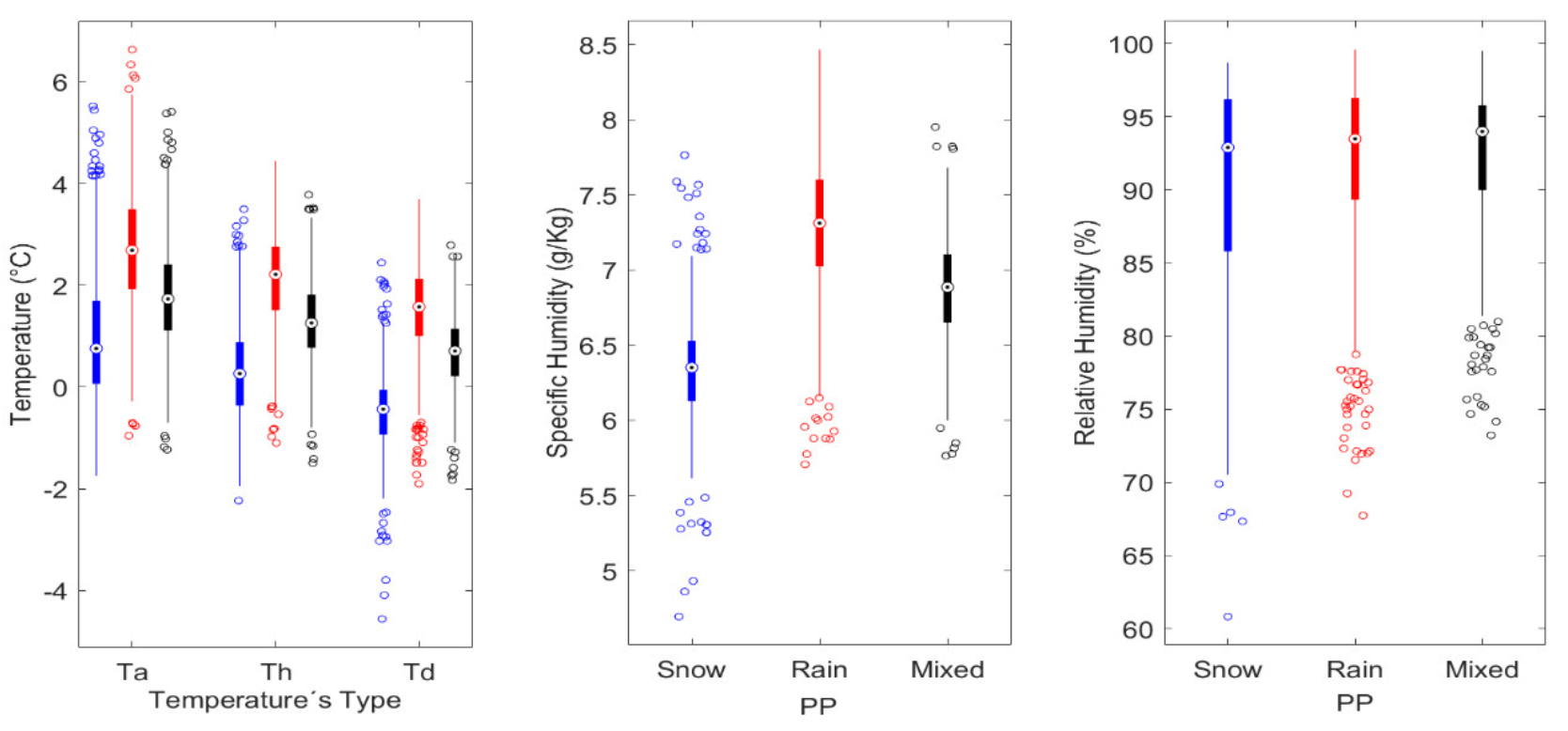
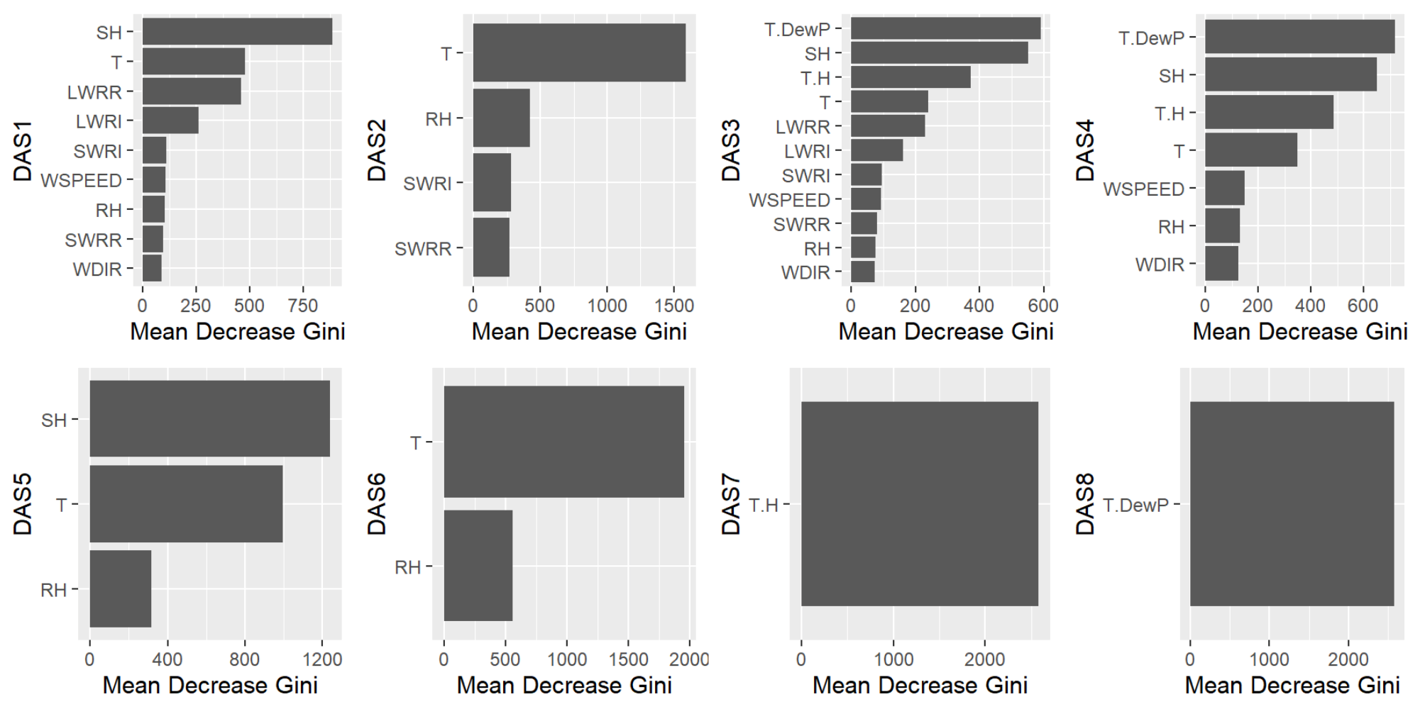
4.2. Meteorological Drivers

For an exploratory analysis in Figure 10, the center and the right plots showed that PP was more sensible to SH than RH. This interpretation assumed that less sensitive PP showed overlapping boxplots, while boxplots showing different ranges of a variable were more sensitive to it. For instance, in Figure 10 (center), the specific humidity showed the lowest values for snow, the highest values for rain, and mixed PP presented intermediate values of specific humidity. Contrarily, in Figure 10 (right), there was not a clear range of relative humidity associated with rain, snow, or mixed PP. This may imply that specific humidity may be a better predictor than relative humidity when considering air moisture related variables.

In Figure 10 (left), Th and Td were indicated to be better predictors than Ta. However, this assumption was still a qualitative one, and a better assessment of meteorological drivers was obtained from the MDG index of RF models.

To derive the meteorological drivers for PP, the MDG obtained from RF was calculated for the eight DASs. In Figure 11, the average value of MDG for each variable is shown. For DAS1, it was clear that specific humidity (SH) was the most important variable when all variables were considered. This was already reflected in the qualitative analysis of Figure 10. For DAS1, SH was followed by air temperature and then by outgoing radiation variables, finally followed by wind speed. Relative humidity was less important than SH as well as wind direction. These results agree with the findings from [47] in relation to the development of an empirical mass balance model for the Antisana glacier; although they used monthly values from reanalysis data only for temperature and wind, they argued that wind may be used as a proxy of moisture flux from the Amazon.

The MDG index for all DASs reflected that, in all cases, temperature and humidity related variables were more important than radiation related variables or wind speed or direction. This result is valuable from a phenomenological perspective because it indicates that monitoring temperature and air moisture content may be useful for surface PP forecasting. Additionally, when air temperature, hydrometeor temperature, and dew point temperature were available, Td was more important than Th, and this was more important than air temperature. This was shown in DAS3 and DAS4. Additionally, when specific humidity and relative humidity were available, specific humidity was more important than relative humidity.

4.3. Development of Parsimonious Logistic Models with Predictors Derived from RF Information

4.3.1. Implementation of Logistic Models Based on AI Knowledge

The results of MDG for all DASs showed that some variables persistently surpassed others in importance. Here, three variables were selected to implement in two LM models, e.g., LM4 was devised with $T_d$ and $S{H}_d$ as independent variables and LM5 with $T_a$ and $S{H}_a$. Afterwards, these models were compared to expert knowledge based classical LMs, LM1 to LM3.

The structures of LM4 and LM5 models are shown in

Table 8. Calibration of parameters for logistic models with predictors derived from RF.

Model	$\mathit{L}\mathit{M}4=\mathit{\alpha }+\mathit{\beta }\ast {\mathit{T}}_{\mathit{d}}+\mathit{\gamma }\ast \mathit{S}\mathit{H}$			$\mathit{L}\mathit{M}5=\mathit{\alpha }+\mathit{\beta }\ast {\mathit{T}}_{\mathit{a}}+\mathit{\gamma }\ast \mathit{S}\mathit{H}$
Parameter	α	β	γ	α	β	γ
Min	38.21	1.05	−14.72	−5.82	−2.30	−0.06
P50	59.57	2.62	−8.55	0.31	−1.92	0.44
Max	101.60	5.57	−5.40	3.55	−1.69	1.37

as well as the calibrated parameters. The MLR optimization returned a wider range for α, β, and γ parameters in model LM4 compared to LM5. This was probably due to the difference in the range of $T_d$ and $T_a$.

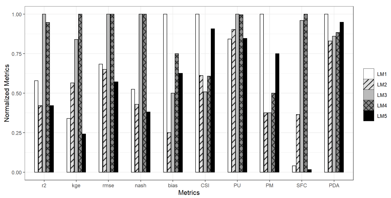
4.3.2. Evaluation of Logistic Models Derived from MDG Predictors

According to Figure 12, LM5 performed better than LM1, LM2, and LM3 in six out of 10 metrics. However, LM4 could not surpass the performance of LM5 despite the use of Td and SH, the most important variables derived from MDG. This model showed, overall, a similar performance to LM3, an expert knowledge-based model. However, the use of SH improved the representation of LM1, which used RH as a humidity related variable.

Although further research is necessary, these results highlight the possibility of “automatic” discovery of predictors by AI models and the conceptual implementation in simpler models. Nevertheless, LM4 did not show a significantly better performance than LM1 to LM3, although a similar performance showed the potentiality of AI-based development of knowledge, which is a limitation of black box models.

To evaluate the performance of LM5 in relation to RF and ANN models, in Figure 13, the normalized metrics are shown. This plot is like Figure 9, where the averages of LM1, LM2, and LM3 are presented. LM5 improved in kge as the best model and also improved for rmse with similar results to RF, surpassing ANN performance and SFC with better results than RF models. These results prove very valuable, because using both predictors selected by MDG improved the performance of parsimonious logistic models, turning information derived from black box models into more transparent models.

5. Discussion

5.1. Models for Precipitation Phase and Predictor Variables

The temperature and the humidity profiles together with the depth of the surface layer control the precipitation phase reaching the ground surface [3]. However, when the surface layer temperatures are close to freezing, and the mixing ratios are neither close to saturation nor very dry, the phase at the surface becomes difficult to forecast. Furthermore, changes in temperature and atmosphere’s saturation can also alter the precipitation phase due to pressure changes driven by changes in vertical air velocity or vertical air movement [48]. The PRAA station fulfills all these conditions due to (1) its altitude near the 0 °C isotherm located between 4800–5100 m.a.s.l [49]; (2) large variability of temperature and specific humidity between days; and (3) strong wind speed around 4.6 m/s with gusts up to 12 m/s [29]. Therefore, models based on both temperature and humidity variables achieved better results to forecast PP, as occurred with LM1 and LM5.

Comparing the calibrated parameters of LM1 with respect to the results presented by [7], the P5–P95 range and the P50 values were very different. This could be related to differences in climatic conditions between inner tropics and the Alps. On the other hand, we computed the rain fraction with P50 calibrated values for LM1 (Table 5) and the mean temperature (2.1 °C) and the relative humidity (81%) of the site (according [29]). Afterwards, it was compared with the rain fraction computed with the mean temperature and the relationship derived by [17] for the Antisana. With the LM1 model, we obtained a rain fraction of 0.83, less than the 0.91 obtained by Wagnon. Thus, the RH inclusion in LM1 decreased the rain fraction with respect to another validated approach based on Ta only.

The current use of Parsivel OTT2 disdrometer is an excellent opportunity to monitor present weather in the site and to explore new approaches to discriminate PP. Since only simple classifications based on temperature are available for the Andes [8,17], these findings will help to improve the knowledge about precipitation in alpine sites of tropical Andes, where solid precipitation is limited to altitudes above 4000 m.a.s.l. Furthermore, the parameters of LM models may be used to obtain solid precipitation, the key variable for glaciological modeling in the inner tropics [2].

The application of RF and ANN allowed us to recognize that only Ta provided a very poor explanation of the PP, while the inclusion of RH or SH improved the performance of LM models. This could be explained due to humidity variations being related to latent heat exchange of hydrometeors during their fall [9]. These facts justify why logistics models using temperature and humidity variables were demonstrated to be the most suitable to explain the sigmoidal S-shaped curve of rain–snow partitioning [7,11,46,50].

5.2. Precipitation Phase Trends and Climate Change

Studies related to PP are almost inexistent in Ecuador despite the important fact that, for instance, the rain to snow ratio represents important information for water resource management and risks related to flash floods occurrence. Due to climate change, the rain to snow ratio is expected to increase, affecting water supply stored as snowpack for one billion people world-wide in winter while also affecting large cities in mountainous tropical regions such as the Andes [1]. Snow falling in the Andes is stored as ice in glaciers and then is released during the dry season, contributing to the base flow. Thus, the buffering effect of glaciers is a vital service during the dry season for water consumption as well as industrial and agricultural uses [51]. Although the retreat in glaciers may not have a great impact in the hydrologic cycle at large scale, due to the buffering effect of wetlands in Ecuador and Perú [1], the change in snowpack may modify the hydrologic functioning of watersheds, wetlands, and groundwater reservoirs in addition to surface drainage [52]. Another aspect that deserves attention is the increasing risk of flash floods occurrence due to increasing rain to snow fraction in CC. However, the change of rain to snow fraction is highly complex in space, depending on several aspects such as topographic features, mean temperature, and snow cover duration, among others [53].

Considering similar thresholds under CC, e.g., −1 and 3, for snow or rain PP, this study showed that temperature and specific humidity are much more important than other variables such as incoming and outgoing radiation or wind. Although it is uncertain, the amount of precipitation in Ecuador is expected to increase due to CC [1,54], but climate models have less uncertainty with temperature, which will raise 4.5–5 °C by the end of this century under “business as usual” type emissions scenarios [55]. Additionally, more moisture is expected to affect the tropical Andes due to enhanced easterlies in CC. Therefore, these changes in the driving variables of PP may affect the processes involved, possibly showing non-linear responses, typically related to phase change processes. Thus, to develop informed base adaptation strategies to CC, more monitoring and studies related to the societal impact of PP change and occurrence are necessary, especially for large cities under increasing need for water provisioning and safety.

6. Conclusions

The dramatic decrease in the ratio of snow to rain due to climate change affects the timing and the duration of the stream flow, affecting the hydrologic cycle and the climate system through complex feedback processes. Therefore, more knowledge about the PP occurrence and the driving mechanisms is necessary. The understanding of these processes is especially important for water management in cities dependent on water coming from glaciers, such as several cities in the Andes, and along other mountain regions around the world.

This study first compared the performance of RF and ANN models in relation to logistic models to derive PP; then, it identified the main drivers of PP occurrence from RF models and finally used these drivers to develop parsimonious logistic models that can help in understanding the underlying processes in relation to PP occurrence. The results showed that RF and ANN outperformed LM in predicting PP in eight out of 10 metrics. Additionally, RF indicated that temperature, dew point temperature, and specific humidity were more important than wind or radiation for PP occurrence. With these predictors, parsimonious and efficient models were developed.

In this research, we presented a pioneering approach in this field. Several advantages of artificial intelligence methods were evident in helping to improve PP forecasting capabilities, identify predictors, and formulate parsimonious models. Thus, information and possibly “knowledge” could be extracted from massive amounts of data, which may complement the existing expert knowledge in this field.

Further work is necessary to evaluate, in other regions, the methodology developed in this study as well findings such as the model structure and the main predictors of PP, which may be specific for the Antisana glacier. Additionally, given the nonlinear response of PP to temperature thresholds, the development and the comparison of models for specific seasons would help to improve our understanding of the physical processes behind PP occurrence.

References

1. Vuille, M. Climate Change and Water Resources in the Tropical Andes; Technical Note No. IDB-TN-515; Inter-American Development Bank: Washington, DC, USA, 2013; Volume 29. [Google Scholar]
2. Favier, V.; Wagnon, P.; Chazarin, J.P.; Maisincho, L.; Coudrain, A. One-Year Measurements of Surface Heat Budget on the Ablation Zone of Antizana Glacier 15, Ecuadorian Andes. J. Geophys. Res. Atmos. 2004, 109, 15. [Google Scholar] [CrossRef] [Green Version]
3. Harpold, A.A.; Kaplan, M.L.; Klos, P.Z.; Link, T.; McNamara, J.P.; Rajagopal, S.; Schumer, R.; Steele, C.M. Rain or Snow: Hydrologic Processes, Observations, Prediction, and Research Needs. Hydrol. Earth Syst. Sci. 2017, 21, 1–22. [Google Scholar] [CrossRef] [Green Version]
4. Vuille, M.; Bradley, R.; Keimig, F. Climate Variability in the Andes of Ecuador and Its Relation to Tropical Pacific and Atlantic Sea Surface Temperature Anomalies. J. Clim. 2000, 13, 2520–2535. [Google Scholar] [CrossRef]
5. Gray, D.M.; Prowse, T.D. The Handbook of Hydrology; Maidment, D., Ed.; McGraw-Hil: New York, NY, USA, 1992; p. 824. ISBN ‎978-0070397323. [Google Scholar]
6. Fassnacht, S.; Kouwen, N.; Soulis, E. Surface Temperature Adjustment to Improve Weather Radar Representation of Multi-Temporal Winter Precipitation Accumulation. J. Hydrol. 2001, 253, 148–168. [Google Scholar] [CrossRef]
7. Froidurot, S.; Zin, I.; Hingray, B.; Gautheron, A. Sensitivity of Precipitation Phase over the Swiss Alps to Different Meteorological Variables. J. Hydrometeorol. 2014, 15, 685–696. [Google Scholar] [CrossRef]
8. L’hôte, Y.; Chevallier, P.; Coudrain, A.; Lejeune, Y.; Etchevers, P. Relationship between Precipitation Phase and Air Temperature: Comparison between the Bolivian Andes and the Swiss Alps/Relation Entre Phase de Précipitation et Température de Air: Comparaison Entre Les Andes Boliviennes et Les Alpes S. Hydrol. Sci. J. 2005, 50, null-997. [Google Scholar] [CrossRef]
9. Harder, P.; Pomeroy, J. Estimating Precipitation Phase Using a Psychrometric Energy Balance Method. Hydrol. Process. 2013, 27, 1901–1914. [Google Scholar] [CrossRef]
10. Feiccabrino, J.; Lundberg, A. Precipitation Phase Discrimination in Sweden. In Proceedings of the 65th Eastern Snow Conference, Fairlee, VT, USA, 28–30 May 2008; pp. 239–254. [Google Scholar]
11. Jennings, K.S.; Winchell, T.S.; Livneh, B.; Molotch, N.P. Spatial Variation of the Rain-Snow Temperature Threshold across the Northern Hemisphere. Nat. Commun. 2018, 9, 1148. [Google Scholar] [CrossRef] [Green Version]
12. Quick, M.C.; Pipes, A. U.B.C. Watershed Model. Hydrol. Sci. J. 1977, 153–162. [Google Scholar] [CrossRef]
13. Kienzle, S.W. A New Temperature Based Method to Separate Rain and Snow. Hydrol. Process. 2008, 22, 5067–5085. [Google Scholar] [CrossRef]
14. Stewart, R.E. Precipitation Types in the Transition Region of Winter Storms. Bull. Am. Meteorol. Soc. 1992, 73, 287–296. [Google Scholar] [CrossRef] [Green Version]
15. Bicknell, B.R.; Imhoff, J.C.; Kittle, J.L., Jr.; Donigian, A.S., Jr.; Johanson, R.C. Hydrological Simulation Program-Fortran: User’s Manual; US Environmental Protection Agency: Athens, GA, USA, 1997.
16. Marks, D.; Winstral, A.; Reba, M.; Pomeroy, J.; Kumar, M. An Evaluation of Methods for Determining During-Storm Precipitation Phase and the Rain/Snow Transition Elevation at the Surface in a Mountain Basin. Adv. Water Resour. 2013, 55, 98–110. [Google Scholar] [CrossRef]
17. Wagnon, P.; Lafaysse, M.; Lejeune, Y.; Maisincho, L.; Rojas, M.; Chazarin, J.P. Understanding and Modeling the Physical Processes That Govern the Melting of Snow Cover in a Tropical Mountain Environment in Ecuador. J. Geophys. Res. Atmos. 2009, 114, 1–14. [Google Scholar] [CrossRef]
18. Lejeune, Y.; Bouilloud, L.; Etchevers, P.; Wagnon, P.; Chevallier, P.; Sicart, J.-E.; Martin, E.; Habets, F. Melting of Snow Cover in a Tropical Mountain Environment in Bolivia: Processes and Modeling. J. Hydrometeorol. 2007, 8, 922–937. [Google Scholar] [CrossRef]
19. Campozano, L.; Célleri, R.; Trachte, K.; Bendix, J.; Samaniego, E. Rainfall and Cloud Dynamics in the Andes: A Southern Ecuador Case Study. Adv. Meteorol. 2016, 2016, 3192765. [Google Scholar] [CrossRef] [Green Version]
20. Ye, H.; Cohen, J.; Rawlins, M. Discrimination of Solid from Liquid Precipitation over Northern Eurasia Using Surface Atmospheric Conditions. J. Hydrometeorol. 2013, 14, 1345–1355. [Google Scholar] [CrossRef] [Green Version]
21. Jennings, K.S.; Molotch, N.P. The Sensitivity of Modeled Snow Accumulation and Melt to Precipitation Phase Methods across a Climatic Gradient. Hydrol. Earth Syst. Sci. 2019, 23, 3765–3786. [Google Scholar] [CrossRef] [Green Version]
22. Aggarwal, S.K.; Goel, A.; Singh, V.P. Stage and Discharge Forecasting by {SVM} and {ANN} Techniques. Water Resour. Manag. 2012, 26, 3705–3724. [Google Scholar] [CrossRef]
23. Francou, B.; Vuille, M.; Favier, V.; Cáceres, B. New Evidence for an ENSO Impact on Low-Latitude Glaciers: Antizana 15, Andes of Ecuador, 0°28′S. J. Geophys. Res. Atmos. 2004, 109, 17. [Google Scholar] [CrossRef]
24. OTT HydroMet. Operating Instructions Present Weather Sensor OTT Parsivel 2; OTT HydroMet: Kempten, Germany, 2016; p. 52. [Google Scholar]
25. Battaglia, A.; Rustemeier, E.; Tokay, A.; Blahak, U.; Simmer, C. PARSIVEL Snow Observations: A Critical Assessment. J. Atmos. Ocean. Technol. 2010, 27, 333–344. [Google Scholar] [CrossRef]
26. Tokay, A.; Wolff, D.B.; Petersen, W.A. Evaluation of the New Version of the Laser-Optical Disdrometer, OTT Parsivel2. J. Atmos. Ocean. Technol. 2014, 31, 1276–1288. [Google Scholar] [CrossRef]
27. Raupach, T.H.; Berne, A. Correction of Raindrop Size Distributions Measured by Parsivel Disdrometers, Using a Two-Dimensional Video Disdrometer as a Reference. Atmos. Meas. Tech. 2015, 8, 343–365. [Google Scholar] [CrossRef] [Green Version]
28. Angulo-Martinez, M.; Begueria, S.; Latorre, B.; Fernández-Raga, M. Comparison of Precipitation Measurements by OTT Parsivel and Thies LPM Optical Disdrometers. Hydrol. Earth Syst. Sci. 2018, 22, 2811–2837. [Google Scholar] [CrossRef] [Green Version]
29. Gualco, L.; Campozano, L.; Robaina, L.; Maisincho, L.; Muñoz, L.; Carlos, J. Corrections of Raindrop Size Distribution Measured by Parsivel OTT 2 Disdrometer under Windy Conditions in Antizana Massif, Ecuador. Water 2021, 13, 2576. [Google Scholar] [CrossRef]
30. Bolton, D. The Computation of Equivalent Potential Temperature. Mon. Weather Rev. 1980, 108, 1046–1053. [Google Scholar] [CrossRef] [Green Version]
31. Garratt, J.R. The Atmospheric Boundary Layer; Cambridge Atmospheric and Space Science Series; Cambridge University Press: Cambridge, UK, 1994; ISBN 9780521467452. [Google Scholar]
32. Koistinen, J.; Saltikoff, E. Experience of Customer Products of Accumulated Snow, Sleet and Rain. Adv. Weather Radar Syst. 1998, 397–406. [Google Scholar]
33. Uyanık, G.K.; Güler, N.N.N.; Uyanik, G.K.; Güler, N.N.N. A Study on Multiple Linear Regression Analysis. Procedia Soc. Behav. Sci. 2013, 106, 234–240. [Google Scholar] [CrossRef] [Green Version]
34. Agatonovic-Kustrin, S.; Beresford, R. Basic Concepts of Artificial Neural Network (ANN) Modeling and Its Application in Pharmaceutical Research. J. Pharm. Biomed. Anal. 2000, 22, 717–727. [Google Scholar] [CrossRef]
35. Du, K.L. Clustering: A Neural Network Approach. Neural Netw. 2010, 23, 89–107. [Google Scholar] [CrossRef]
36. Stangierski, J.; Weiss, D.; Kaczmarek, A. Multiple Regression Models and Artificial Neural Network ({ANN}) as Prediction Tools of Changes in Overall Quality during the Storage of Spreadable Processed Gouda Cheese. Eur. Food Res. Technol. 2019, 245, 2539–2547. [Google Scholar] [CrossRef] [Green Version]
37. Jain, A.; Kumar, A.M. Hybrid Neural Network Models for Hydrologic Time Series Forecasting. Appl. Soft Comput. 2007, 7, 585–592. [Google Scholar] [CrossRef]
38. Sarica, A.; Cerasa, A.; Quattrone, A. Random Forest Algorithm for the Classification of Neuroimaging Data in Alzheimers Disease: A Systematic Review. Front. Aging Neurosci. 2017, 9, 329. [Google Scholar] [CrossRef] [PubMed]
39. Breiman, L. Random forests. Mach. Learn. 2001, 45, 5–32. [Google Scholar] [CrossRef] [Green Version]
40. Ali, J.; Khan, R.; Ahmad, N.; Maqsood, I. Random Forests and Decision Trees. Int. J. Comput. Sci. Issues 2012, 9, 272–278. [Google Scholar]
41. Liaw, A.; Wiener, M. Classification and Regression by RandomForest. R News 2002, 2, 18–22. [Google Scholar]
42. Tyralis, H.; Papacharalampous, G.; Langousis, A. A Brief Review of Random Forests for Water Scientists and Practitioners and Their Recent History in Water Resources. Water 2019, 11, 910. [Google Scholar] [CrossRef] [Green Version]
43. Knoben, W.J.M.; Freer, J.E.; Woods, R.A. Technical Note: Inherent Benchmark or Not? Comparing Nash-Sutcliffe and Kling-Gupta Efficiency Scores. Hydrol. Earth Syst. Sci. 2019, 23, 4323–4331. [Google Scholar] [CrossRef] [Green Version]
44. Nicodemus, K.K. Letter to the Editor: On the Stability and Ranking of Predictors from Random Forest Variable Importance Measures. Brief. Bioinform. 2011, 12, 369–373. [Google Scholar] [CrossRef] [Green Version]
45. Calle, M.L.; Urrea, V. Letter to the Editor: Stability of Random Forest Importance Measures. Brief. Bioinform. 2010, 12, 86–89. [Google Scholar] [CrossRef] [Green Version]
46. Casellas, E.; Bech, J.; Veciana, R.; Pineda, N.; Rigo, T.; Miró, J.R.; Sairouni, A. Surface Precipitation Phase Discrimination in Complex Terrain. J. Hydrol. 2021, 592, 125780. [Google Scholar] [CrossRef]
47. Manciati, C.; Villacis, M.; Taupin, J.-D.; Cadier, E.; Galárraga-Sánchez, R.; Cáceres, B. Empirical Mass Balance Modelling of South American Tropical Glaciers: Case Study of Antisana Volcano, Ecuador. Hydrol. Sci. J. 2014, 59, 1519–1535. [Google Scholar] [CrossRef] [Green Version]
48. Thériault, J.M.; Stewart, R.E. On the Effects of Vertical Air Velocity on Winter Precipitation Types. Nat. Hazards Earth Syst. Sci. 2007, 7, 231–242. [Google Scholar] [CrossRef] [Green Version]
49. Basantes-Serrano, R.; Rabatel, A.; Francou, B.; Vincent, C.; Maisincho, L.; Cáceres, B.; Galarraga, R.; Alvarez, D. Slight Mass Loss Revealed by Reanalyzing Glacier Mass-Balance Observations on Glaciar Antisana 15 (Inner Tropics) during the 1995–2012 Period. J. Glaciol. 2016, 62, 124–136. [Google Scholar] [CrossRef] [Green Version]
50. Fehlmann, M.; Gascón, E.; Rohrer, M.; Schwarb, M.; Stoffel, M. Estimating the Snowfall Limit in Alpine and Pre-Alpine Valleys: A Local Evaluation of Operational Approaches. Atmos. Res. 2018, 204, 136–148. [Google Scholar] [CrossRef]
51. Jomelli, V.; Khodri, M.; Favier, V.; Brunstein, D.; Ledru, M.P.; Wagnon, P.; Blard, P.H.; Sicart, J.E.; Braucher, R.; Grancher, D.; et al. Irregular Tropical Glacier Retreat over the Holocene Epoch Driven by Progressive Warming. Nature 2011, 474, 196–199. [Google Scholar] [CrossRef] [Green Version]
52. Mark, B.G.; Bury, J.; McKenzie, J.M.; French, A.; Baraer, M. Climate Change and Tropical Andean Glacier Recession: Evaluating Hydrologic Changes and Livelihood Vulnerability in the Cordillera Blanca, Peru. Ann. Assoc. Am. Geogr. 2010, 100, 794–805. [Google Scholar] [CrossRef]
53. López-Moreno, J.I.; Pomeroy, J.W.; Morán-Tejeda, E.; Revuelto, J.; Navarro-Serrano, F.M.; Vidaller, I.; Alonso-González, E. Changes in the Frequency of Global High Mountain Rain-on-Snow Events Due to Climate Warming. Environ. Res. Lett. 2021, 16, 94021. [Google Scholar] [CrossRef]
54. Campozano, L.; Ballari, D.; Montenegro, M.; Avilés, A. Future Meteorological Droughts in Ecuador: Decreasing Trends and Associated Spatio-Temporal Features Derived From {CMIP}5 Models. Front. Earth Sci. 2020, 8, 17. [Google Scholar] [CrossRef]
55. Bradley, R.S.; Vuille, M.; Diaz, H.F.; Vergara, W. Threats to Water Supplies in the Tropical Andes. Clim. Chang. Sci. 2006, 312, 1755. [Google Scholar] [CrossRef]
Figure 1. Location map of monitoring stations used for the Antisana glacier 12. (a) Antisana glacier in the northern Andes of Ecuador, (b) Moraine basin, (c,d) PRAA-Morrena station for two seasons, November 2017, and June 2019, respectively.
Water 13 03022 g001
Figure 2. Flowchart of the methodology.
Water 13 03022 g002
Figure 3. Plots of T a , T h , T d (from top to bottom) shown for solid, mixed, and liquid precipitation (from left to right). The “S” curves in cyan were plotted from the observed data, and the black curves were plotted with data after multidimensional K–means outliers’ detection. Temperature class is in the horizontal axis in all plots and is represented by the median value per bin.
Water 13 03022 g003
Figure 4. Artificial neuron with inputs Xi, output y, and activation function f (left) as well as artificial neural network with three layers (shallow network). The hidden and the output layers used specific case transfer functions (right).
Water 13 03022 g004
Figure 5. Example of how a decision tree in RF works.
Water 13 03022 g005
Figure 6. Precipitation phase plots using logistic models. From left to right. LM1 depends on Ta and RH (left). LM2 depends on Th (center). LM3 depends on Td (right). The black points represent observed values, and the red lines represent simulated values.
Water 13 03022 g006
Figure 7. Precipitation phase plots using artificial neural networks for DAS1 to DAS8 from left to right and from top to bottom. The black dots represent observed values, and the red lines represent the simulations by ANN models.
Water 13 03022 g007
Figure 8. Precipitation phase plots using RF for DAS1 to DAS8 from left to right and from top to bottom. The black dots represent the observed values, and the red lines represent the simulated values.
Water 13 03022 g008
Figure 9. Normalized metrics for LM, ANN, and RF models. The values are normalized indexes and the range is [0–1] where the best scores are closer to 0. Fraction quantifications are in lowercase and detection in uppercase.
Water 13 03022 g009
Figure 10. Boxplots of Ta, Th, and Td are shown for solid, liquid, and mixed precipitation (blue, red, black) (left). Boxplots of specific humidity are shown for snow, rain, and mixed precipitation (blue, red, black) (center). Boxplots of relative humidity are shown for snow, rain, and mixed precipitation (blue, red, black) (right).
Water 13 03022 g010
Figure 11. Identification of precipitation phase meteorological drivers (variables) using RF. The mean decrease Gini index is compared for this purpose for each DAS, DAS1 to DAS8, from left to right and from top to bottom.
Water 13 03022 g011
Figure 12. Normalized metrics (quantification and detection s) for the mean of all the classic logistic models. For normalized indexes, the range is [0–1], where the best model has a value of 0.
Water 13 03022 g012
Figure 13. Normalized metrics for LM5, ANN, and RF models. Normalized indexes range is [0–1], where 0 is the best model.
Water 13 03022 g013