
Global Sensitivity Analysis of Groundwater Related Dike Stability under Extreme Loading Conditions


1
Department of Physical Geography, Faculty of Geosciences, University of Utrecht, P.O. Box 80115, 3508 TC Utrecht, The Netherlands
2
Unit Soil and Groundwater Systems, Deltares, P.O. Box 85467, 3508 AL Utrecht, The Netherlands
*
Author to whom correspondence should be addressed.
Water 2021, 13(21), 3041; https://doi.org/10.3390/w13213041
Submission received: 21 September 2021
/
Revised: 25 October 2021
/
Accepted: 26 October 2021
/
Published: 1 November 2021
(This article belongs to the Section Hydrogeology)
Abstract
:With up to 15% of the world’s population being protected by dikes from flooding, climate-change-induced river levels may dramatically increase the flood risk of these societies. Reliable assessments of dike stability will become increasingly important, but groundwater flow through dikes is often oversimplified due to limited understanding of the important process parameters. To improve the understanding of these parameters, we performed a global sensitivity analysis on a comprehensive hydro-stability model. The sensitivity analysis encompassed fifteen parameters related to geometry, drainage conditions and material properties. The following three sensitivity settings were selected to characterize model behavior: parameter prioritization, trend identification and interaction qualification. The first two showed that dike stability is mostly dependent on the dike slope, followed by the type of subsurface material. Interaction quantification indicated a very prominent interaction between the dike and subsurface material, as it influences both groundwater conditions and dike stability directly. Despite our relatively simple model setup, a database containing the results of the extensive Monte Carlo analysis succeeded in finding most of the unsafe sections identified by the official inspection results. This supports the applicability of our results and demonstrates that both geometry and subsurface parameters affect the groundwater conditions and dike stability.
1. Introduction
Over 45 major flood events occurred in Europe between 1950 and 2005 that each resulted in more than 70 fatalities or a collected economic damage of EUR 7.6 × 10¹⁰ [1]. As a result, many flood prone areas have an extensive network of artificially elevated levees or dikes, which, along Europe’s major rivers, add up to a length of approximately 60,000 km [2]. To ensure the safety of people living behind dikes, continuous maintenance and reinforcements are needed to warrant the stability of dikes and their proper functioning during high water events. Climate change, e.g., earlier snow melt or an increase in extreme precipitation events in the upstream drainage area [3], poses a new threat that may increase the risk of a society to flooding [4]. To maintain safety levels under changing climatic conditions, major investments are needed for dike maintenance and reinforcement, of which the costs for the latter are in the order of EUR 1–20 million per kilometer [1]. Improved knowledge of the processes during and following a high-water event that can result in dike failure is crucial for more cost-effective dike reinforcements, which may reduce the total expenditures on dike reinforcements substantially and can support more societally acceptable flood defense measures [5].
Many dike failure mechanisms are related to local groundwater conditions and pore pressures in the dike body. In response to elevated river stages, changing groundwater conditions may increase the pore pressure and, thus, reduce the effective normal strength, while, at the same time, the lateral load of river water pushing against the dike is increased. Therefore, parts of its inner or outer slope may slip, or the dike may slide along its base (soil slip sensu lato), threatening the structural integrity of the dike. Accordingly, when analyzing a dike failure hazard in relation to high groundwater levels and river stages, multiple failure mechanisms must be considered.
Although we acknowledge that critical groundwater heads in dikes are primarily driven by the occurrence and nature of high-water events, their variation in space and time also depends on surface geometry and subsurface properties. Previous research on this topic can roughly be divided into the following three categories: research focusing purely on hydrology, research focusing on single cases or research assessing variability in either surface geometry or subsurface properties. An extensive analysis on only the hydrology near a river dike was provided [6,7]. Research on a single case [8] was often also focused on the effect of artificial reinforcements [9,10]. Attempts including a local sensitivity analysis investigated the influence of material properties [11] or geometry [12] on the stability of embankments. In sum, none of these previous studies conducted a full analysis that considers both variations in hydrological parameters as factors influencing the stability of a dike.
Such a full analysis has already been widely applied in landslide probability modelling [13,14,15]. Nonetheless, whereas slope hydrology is mostly dependent on rainfall infiltration, flow as a result of elevated river water levels mostly occurs horizontally and is often affected by intersecting aquitards, resulting in very different patterns of groundwater flow and pore pressure buildup. These differences inhibit the direct application of results from landslide modelling to river dike failure scenarios. Nonetheless, to assess variations in hydrological parameters as factors influencing the stability of a dike, a comprehensive hydro-stability system needs to be modelled.
To quantify the model and parameter uncertainty, local sensitivity approaches estimating the partial derivatives of the model at a specific point in the parameter space are no longer sufficient [16]. Alternatively, a global sensitivity analysis can handle nonlinearity and local variations expected in more complex models. A global sensitivity analysis considers the entire variation of the input factors [17]. Global sensitivity analysis recently gained interest in environmental modelling [18], and the different goals and methods related to global sensitivity in environmental models have been extensively reviewed [19,20]. Hydrological models have seen a similar rise in interest for global sensitivity analysis, both from a methodological point of view [21,22,23] and for analyzing geo-hydrological systems [24] and slope stability uncertainty [25,26,27]. Though some attempts have been made to analyze the global sensitivity of dike stability based on the uncertainty in its internal characteristics [11,25], no complete sensitivity analysis covering both geometrical as subsurface characteristics has yet been made.
Thus, to assess both geometrical and subsurface characteristics of dikes, we created a coupled high-resolution groundwater model and a limit equilibrium stability analysis. To constrain our results and to highlight first-order relationships, we evaluated the stability under the most critical loading conditions and the maximum pore water pressures. Three failure mechanisms that affect the macro-stability of a dike were considered, being inner slope stability, outer slope stability and basal sliding, as their occurrence is directly linked to the geometry of a dike and its composition.
To add to previous research on both river dike hydrology and global sensitivity analysis, the goal of our analysis was to identify the overall stability of a dike in terms of its factor of safety F under different hydrological loading conditions, subsurface geometries and material properties, and including pore pressure calculations. In this work, our research goal translates into the following three sensitivity settings to characterize model behavior: parameter prioritization, trend identification and interaction qualification. We aim to provide insights in each of these settings, while maintaining a reasonable computation time. For parameter prioritization we used the Elementary Effect [28] and the delta-importance measure [29]. As we are mostly interested in those factors that could lead to unstable dikes, we used a regional sensitivity analysis (RSA) to perform trend identification and identify regions in the parameter space with a safety factor below one. For interaction qualification, we focused on the subsurface, and used response surfaces to analyze the interaction activate between hydrology, material characteristics and dike stability. Moreover, the outcome of this global sensitivity analysis can be used to inform semi-qualitative assessments of dike stability as often applied in regional inventories, and the conducted set of model runs is used for a direct comparison to a case study site in the Netherlands.
2. Materials and Methods
2.1. Case-Study Schematization
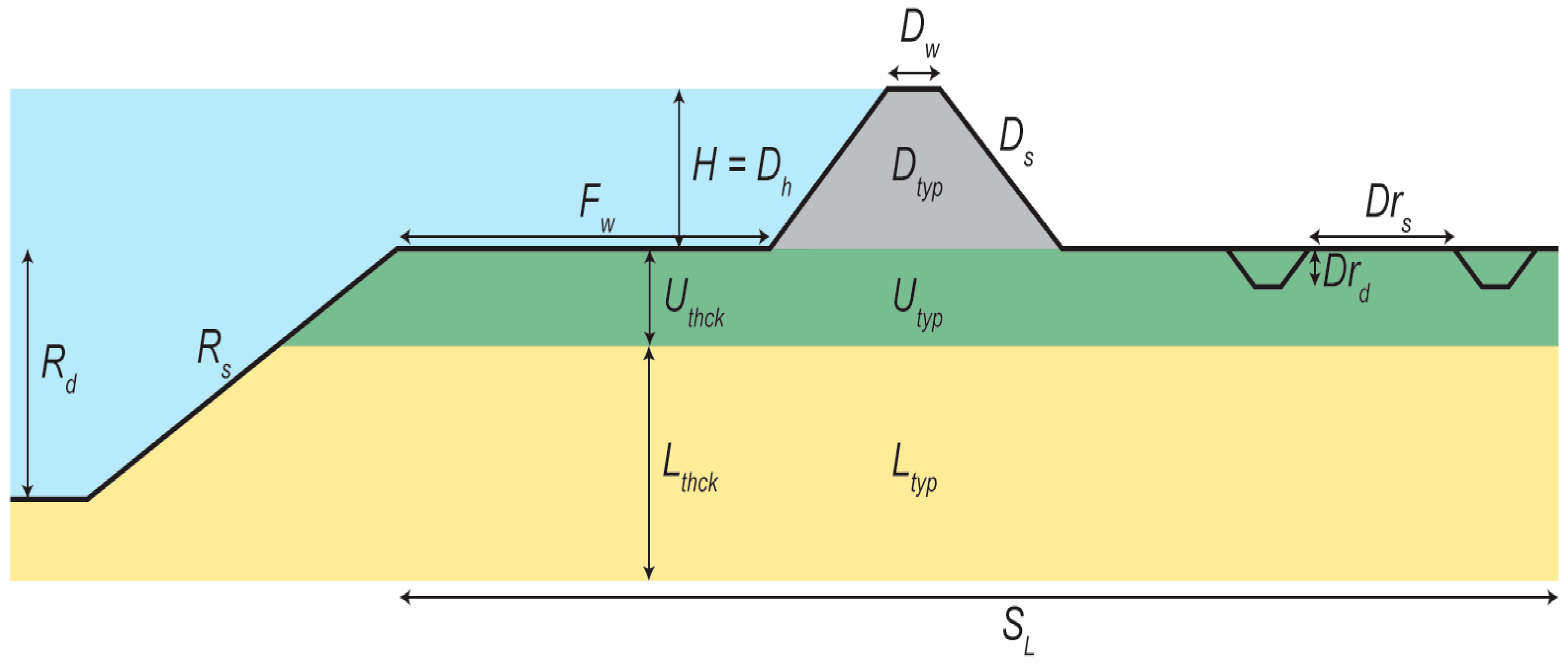
We applied the global sensitivity analysis on a cross-section from the river to the hinterland behind the dike. Fifteen parameters (Table 1) describe the cross-section, subdivided in the following three groups: topographical parameters, subsurface parameters and human management parameters. The topography is described by the following six parameters: the dike height (), dike crest width (), dike slope () and floodplain width (), riverbed slope () and river depth () (Figure 1). The subsurface is described by five parameters, which divide the subsurface in three units with uniform characteristics. The dike is schematized by its material type (), in addition to the previously mentioned geometry parameters , and . The upper subsurface layer is schematized by a thickness () and material type (). The same applies to the lower subsurface layer (, ). Two parameters describe human management by specifying the drainage conditions behind the dike (Figure 1), which are drain spacing () and drainage depth ().
2.2. Coupled Hydrology-Stability Model
2.2.1. Hydrological Model Setup
We added a stability module to a groundwater model to examine the stability of the schematized cross-section. The MODFLOW 6 software [30,31], a Modular Three-Dimensional Finite-Difference Groundwater Flow Model, simulates the groundwater conditions, which are included in the structural stability using the Generalized Limit Equilibrium Method (GLEM) [32,33]. The MODFLOW 6 hydrological model is constrained by the river water level and drainage depth. On the river side, the imposed river stage at the top of the dike constitutes a head-controlled boundary condition that is regulated by the MODFLOW river package. A head-controlled boundary on the inner side of the dike is regulated by the MODFLOW drain package, which creates outflow-only seepage points [30]. Seepage is possible if the hydraulic head at the surface is higher than the surface elevation. In addition, at a distance of behind the dike, a ditch is located with a depth of (Table 1), enabling faster drainage of deeper layers. The cell size is 0.5 m in all directions, which enables the assessment of small-scale spatial variation while retaining the computational efficiency needed. The model first performed a steady-state simulation, in which the river stage () was set at the dike crest elevation. It was assumed that under these conditions, the pore pressures reach their most critical values. After the steady-state simulation, a rapid drawdown of from the dike crest to the dike toe in a time period () of one day was transiently simulated with a 3-hour timestep. As pore pressures in the dike do not immediately follow river water level changes and the stabilizing effect of the high river water levels is absent, these conditions might provoke outer slope failure. An exploratory sensitivity analysis showed a time step of 3 h does not significantly impact results when compared to smaller time steps.
2.2.2. Dike Slope Stability Model Setup
Dike stability is expressed by the factor of safety (), which is calculated separately for inner slope failure, basal sliding and outer slope failure using the Generalized Limit Equilibrium Method [32,33], resulting in the following three safety factors: , , . This method solves both moment and force equilibrium on a slip surface for different ratios between the vertical and horizontal inter-slice shear forces. The relationship between the magnitude of the inter-slice shear and normal forces is assumed to be constant [34]. The factors of safety presented in this paper always represent the factor of safety of the most critical circular slip surface, derived by an effective critical slip surface minimization technique adapted from [35]. To constrain the slip surface for inner and outer sliding the slip surface is forced to enter on the dike crest or on the corresponding dike side. For basal sliding an infinite slump radius is assumed, which results in a horizontal slip surface and enables the calculation of using only force equilibrium. To ignore very small slumps not causing dike breaches, a minimum cross-sectional slip surface area of 5 m2 is imposed.
2.3. Workflow and Parameters for Global Sensitivity Analysis
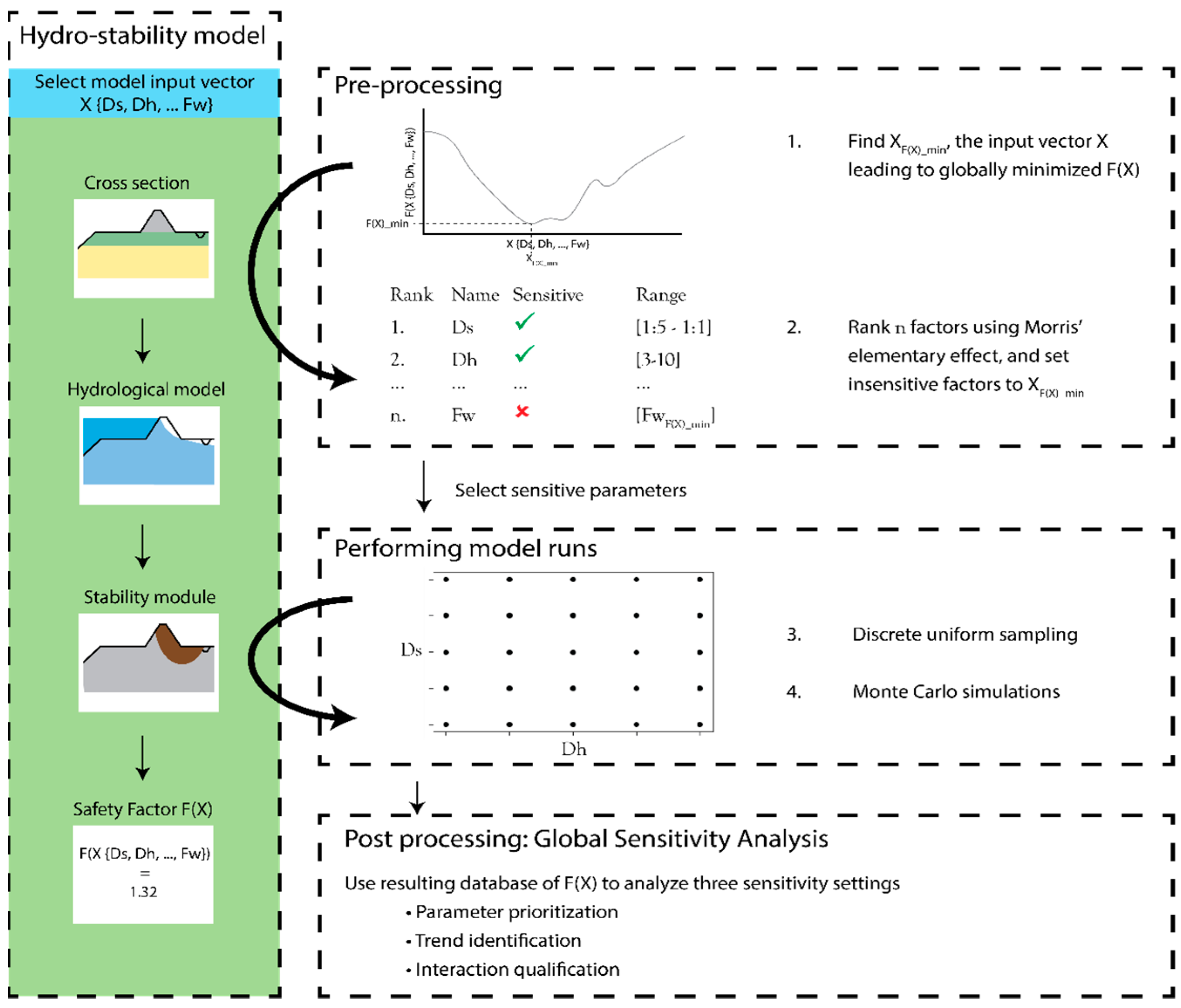
As conducting the entire global sensitivity analysis with all parameters was not a feasible option due to increasing computation times, we first screened our inputs using the Elementary Effect test (EE) [28,36]. Hereby, we identified which input parameters have a small contribution to the output variation in high-dimensional models and can, therefore, be set to a fixed value. Subsequently, the global sensitivity analysis was performed using a Monte-Carlo (MC) approach, as it captures the entire range of possible combinations, while facilitating parameter interaction understanding (Figure 2). The Delta Moment-Independent measure (DMI) [29] was used to quantify the sensitivity of the factors contributing significantly to the variation in the model output.
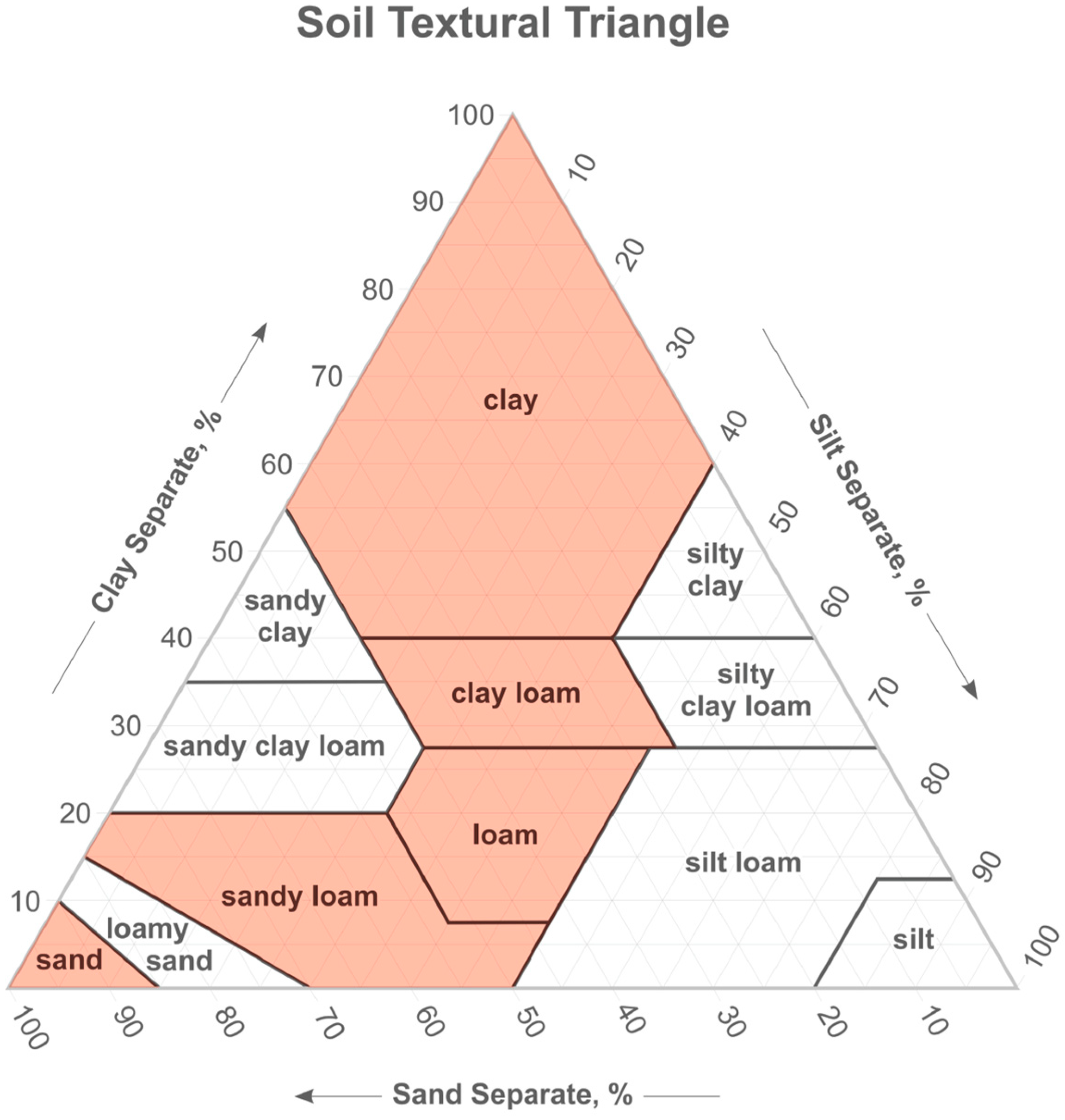
All variable parameters defining the cross-section are screened using the Elementary Effect test (EE). As no information is available a priori, the parameters are sampled from a uniform distribution within their possible range (Table 1). The material types (, , ) each represent a single lithological class (Figure 3), having deterministic attributes used in the coupled hydrology-stability model. We selected the values for these attributes (Table 2) based on characteristic values in the literature. The hydraulic conductivity () is derived from the geometric mean of multiple laboratory measurements of soils with a relatively high density [37]. The cohesion (), the effective friction angle (), the bulk unit weight () and the saturated bulk unit weight () are in line with the European standardized characteristics for soil stability [38].
2.4. Parameter Prioritization
This sensitivity setting focusses on identifying the input factor (parameter) that has the largest effect on the model output, e.g., the input factor that, when fixed, decreases output variability the most. For this, we used the Elementary Effect test (EE) and the Delta Moment-Independent measure (DMI).
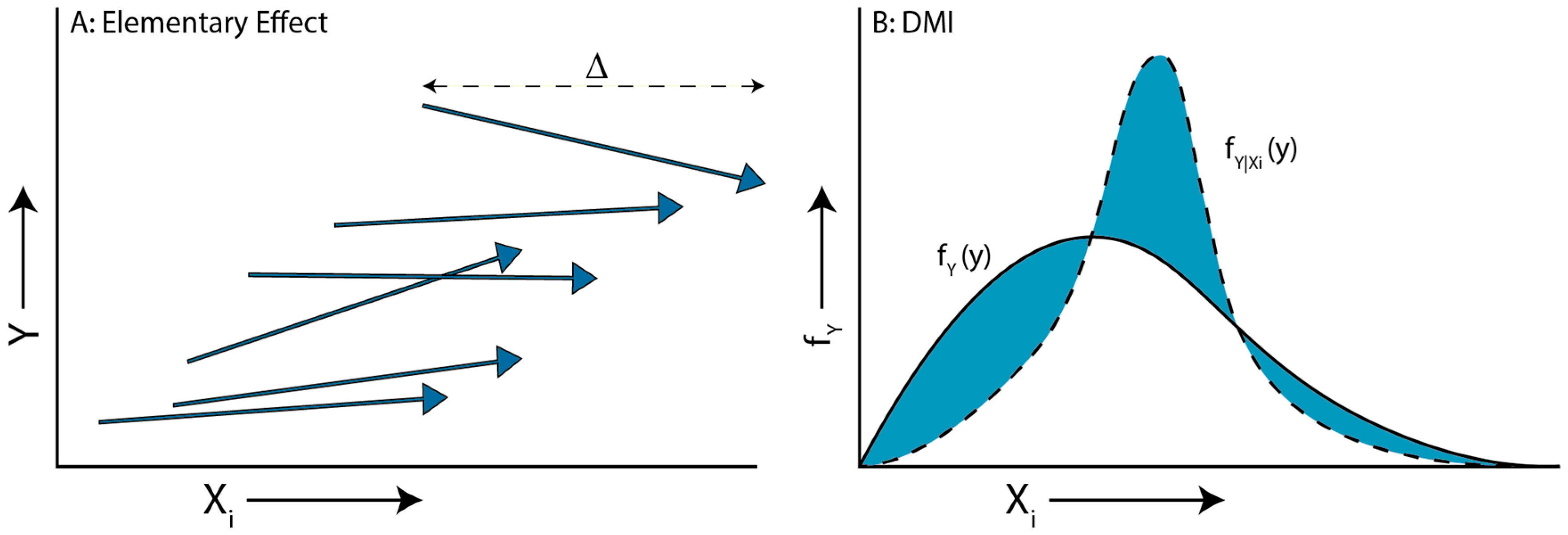
The Elementary Effect test [36] is an effective sensitivity analysis (SA) method that is widely used for screening practices, as it provides relatively good results at small sample sizes [28]. This method is basically a One-At-a-Time analysis, which is extended to the full input factor space. The original method [28] measures sensitivity in terms of , indicating the first order influence or elementary effect, and , indicating second order influences, being nonlinearity or interaction effects. For each input factor, random baseline points are selected from which the other are varied (Figure 4A). Given function “” (in our case the calculation of ), step size and a random baseline sample the elementary effect of input factor is given by
The final for any input factor is the mean of the at all baseline points . Non-monotonic models result in both positive and negative ’s for a given input factor, which average out when taking the mean. Therefore, [36] introduced , which is the mean of all absolute elementary effects and is found to be suitable for input factor ranking.
where is the elementary effect for input factor using the -th step with step size , with r being the number of steps in the parameter space. A value near zero indicates that the parameter has a small general effect on the output. This measure is used in the Insensitive Factor fixing procedure.
The Delta Moment-Independent measure (DMI) [29] is based on shifts in the probability density function , contrary to most SA techniques, which are variance-based. Variance-based sensitivity, according to classical utility theory, is not suitable to describe uncertainty in case of a non-normal probability distribution and in case of a non-quadratic utility function. Moreover, the probability density function provides a more complete overview of sensitivity than variance-based techniques. DMI returns the measure (), which represents the non-overlapping area between an unconditional input vector , including all parameter values, and a conditional input vector , consisting of a subset of parameter values (Figure 4B). Mathematically, it is expressed as:
with
which shows that the input factor specific depends on the shift in probability density function for multiple conditional inputs and on the underlying probability of that shift to occur. As in our method, a uniform probability function is used, and the mean of the separate shifts represents the final .
2.5. Factor Fixing Procedure
Factor fixing is often used as a SA setting in itself, where the goal is to simplify model and prevent overparameterization [23]. In this research, it was just a means by which we aimed to keep MC simulation runs to an acceptable level, i.e., by fixing the least influential parameters to some nominal value. To provide evidence for the identification of the least influential parameters for the model output, we used an iterative version of the SA repeatability test [40], previously successfully adapted for environmental models [41,42]. This approach focusses on testing the predictive capacity of parameters.
First, 1200 samples of all model parameters are created. The test then consists of the comparison of two conditional input samples, and to the previously created unconditional sample, . Set fixes the input factors deemed insensitive at a predetermined value, while fixes the input factors deemed sensitive. Afterward, the unconditional result is compared with the conditional results and . If a correct classification of important and non-important parameters was used, the correlation coefficient () between and approaches 1, while the correlation coefficient of and approaches 0, as the parameters fixed in should have a small influence on the results. We iteratively applied this approach, starting with only the most important factor classified as sensitive, and consecutively also classifying the next important parameter as sensitive, until the correlation coefficient exceeds a certain threshold. A threshold of 0.95 has been successfully applied [41] to limit the dimensionality of a problem, while retaining sufficient model variability.
To initially rank the parameters from sensitive to insensitive, we used the enhanced Elementary Effects method [36] on the initial sample X1. The iteration was performed for each failure mechanism separately, but we used an inclusive selection strategy, indicating that only those parameters that were found to be insensitive for all failure mechanisms were excluded from the MC-parameters. Although the inclusive approach increases the dimensionality of our problem, it also enables an easy comparison between the different failure mechanisms. As we used a threshold for of 0.95 as closing criterion for the iterative Factor Fixing procedure, this threshold being lower than 1 indicated that the factors to be fixed still influenced the model outcome, though their influence was limited. As this research was investigating worst case scenarios, any factor to be fixed should have been set at a value that resulted in relatively low safety factors. This value is selected from the input vector that results in the globally minimized within the specified parameter ranges (Table 3) for each failure mechanism separately. Initiated at a random starting point, a modification of Powell’s method [43] performs the minimization operation. This method performs a bi-directional search in one dimension, meaning it searches for the local minimum by changing only one input parameter. The input parameter is updated to the value resulting in the minimum , and the bi-directional search is applied to the next input factor. After minimizing all input factors, the intermediate model output is stored, and the first factor is again selected. When the difference between the previous and current intermediate output is lower than a given threshold, the globally minimized input vector is found. Though we acknowledge that fixing only a single input factor to value in the globally minimized input vector does not necessarily result in the local minimum at any given point in the parameter space, we believe that it results in a safety factor near the real minimum at that point.
2.6. Factor Sampling
As neither the real parameter probability density functions of the selected model parameters were known and no information was available on their correlation, we used a uniform uncorrelated sampling strategy. The sensitive factors were sampled using a discrete uniform distribution in their possible range (Table 1), which suggested a known, finite number of outcomes that were equally plausible. We used five steps () at which to sample discrete values from the minimum value () to the maximum value () in the possible range given parameter , i.e.,
Afterwards, each possible combination of the parameter values was selected for the MC analysis, resulting in a number of model runs, with being the number of selected parameters.
2.7. Trend Identification and Interaction Qualification
For trend identification and to increase our understanding of model sensitivity, we explored whether any change toward higher parameter values would also lead to a larger safety factor. To this end, we performed a regionalized sensitivity analysis (RSA), which aimed to identify regions in the inputs space that result in an output in a specified zone [23]. In our case, the selected zone was , as it was intuitively the most interesting region of model outcomes; that of dike failure. To indicate this regional effect, we used as a measure, which is the probability for a fixed parameter to result in given the variations of the other parameters. This measure can be easily calculated as a result of the uniform discrete sampling distribution. Interaction qualification uses response surfaces, which directly show the correlation between material properties, groundwater and dike stability. As we focused on a qualitative description and interpretation of these interactions, no quantitative statistical measures were used.
3. Results
3.1. Exemplary Results of the Hydro-Stability Model
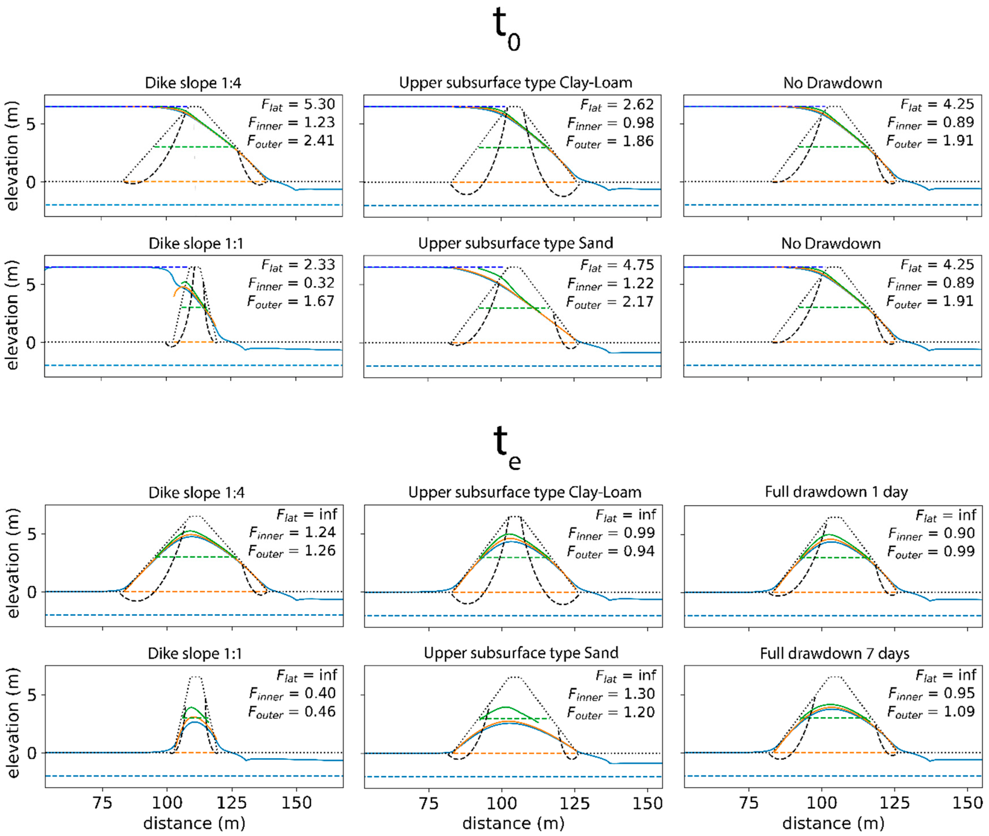
The typical model results that highlight the interplay between the model input factors, groundwater hydrology and macro-stability are presented in Figure 5. Focusing on changes in groundwater conditions, the phreatic surface in the dike after the steady-state simulations () seems to be more influenced by dike geometry than material properties. Due to increased drainage, steeper and narrower dikes seem to result in a generally lower phreatic level, as the hydraulic heads at the center of the dike are more directly affected by gradient changes near the surface. Lower river water levels after draw-down also affect the phreatic level, but the amount of lowering depends on the possibility to drain the excess pore pressure. This is reflected in lower groundwater levels at steeper and thus smaller dikes, at dikes on a sandy substrate and in case of longer drawdown times.
For inner slope stability, these results have a more direct effect, as the minimum factors of safety are always found at , when the pore pressures are the highest. For basal sliding, this is the case as well, although this is also influenced by the still high river water levels, which apply a lateral force. As a result, the dike’s stability related to basal sliding increases to infinity at , as the river water level is at the dike toe and no driving force is exerted by it. For outer slope stability, the opposite argument applies, and due to a decrease in the lateral river water pressure, the lowest is most often found at (Figure 5).
These example results clearly show that not only the safety factor, but also the slip surface area and location are dependent on the hydrological conditions. Higher pore pressures are likely to result in larger slumps that result in a greater chance of dike breach, in addition to lower stability. The results also indicate an effect of drawdown time, which is related to the flood wave shape, but in this study the drawdown time () was kept constant.
3.2. Parameter Priorization
3.2.1. Factor Fixing on Globally Minimized Input Vector
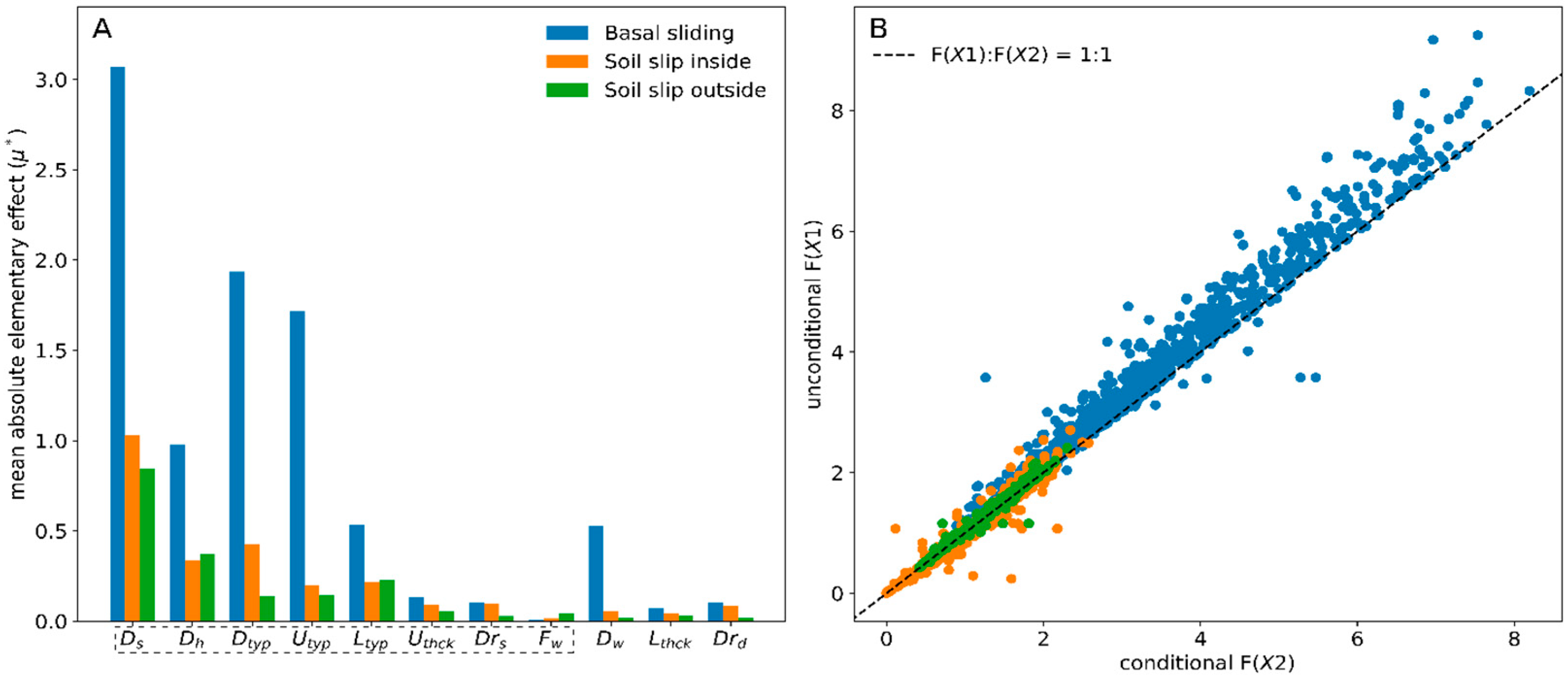
The values used to fix the insensitive factors are derived from the input vector that results in the globally minimized . The globally minimized factors of safety () are 0.69, 0.00 and 0.26 for basal sliding, inner slope stability and outer slope stability, respectively, of which the corresponding input vectors are shown in Table 3. The iterative factor fixing is performed in the order of the mean absolute elementary effect () of each input factor per failure mechanism (Figure 6A). If the dike slope, dike height, dike material type, upper subsurface type, lower subsurface type, upper subsurface thickness, drainage spacing and foreland width are classified as sensitive, the for all the failure mechanisms. These eight factors (Figure 6) are, thus, selected for the MC-analysis. Using the final and , a mean error in of −2.76·, 7.86· and −1.81· and a of 0.965, 0.950 and 0.986 are observed for basal sliding, inner slope stability and outer slope stability, respectively, and a combined of 0.985 across all the failure mechanisms. Based on these small errors and the high correlation coefficient, the drainage depth, lower layer thickness and dike crest will be fixed. Furthermore, most points in Figure 6B are above the 1:1 line, indicating that fixing these input factors either results in equal or lower factors of safety, which suits our goal of performing a sensitivity analysis under the most critical conditions and justifies the use of the global minimum as the fixing point.
3.2.2. Delta Moment Independent Measure
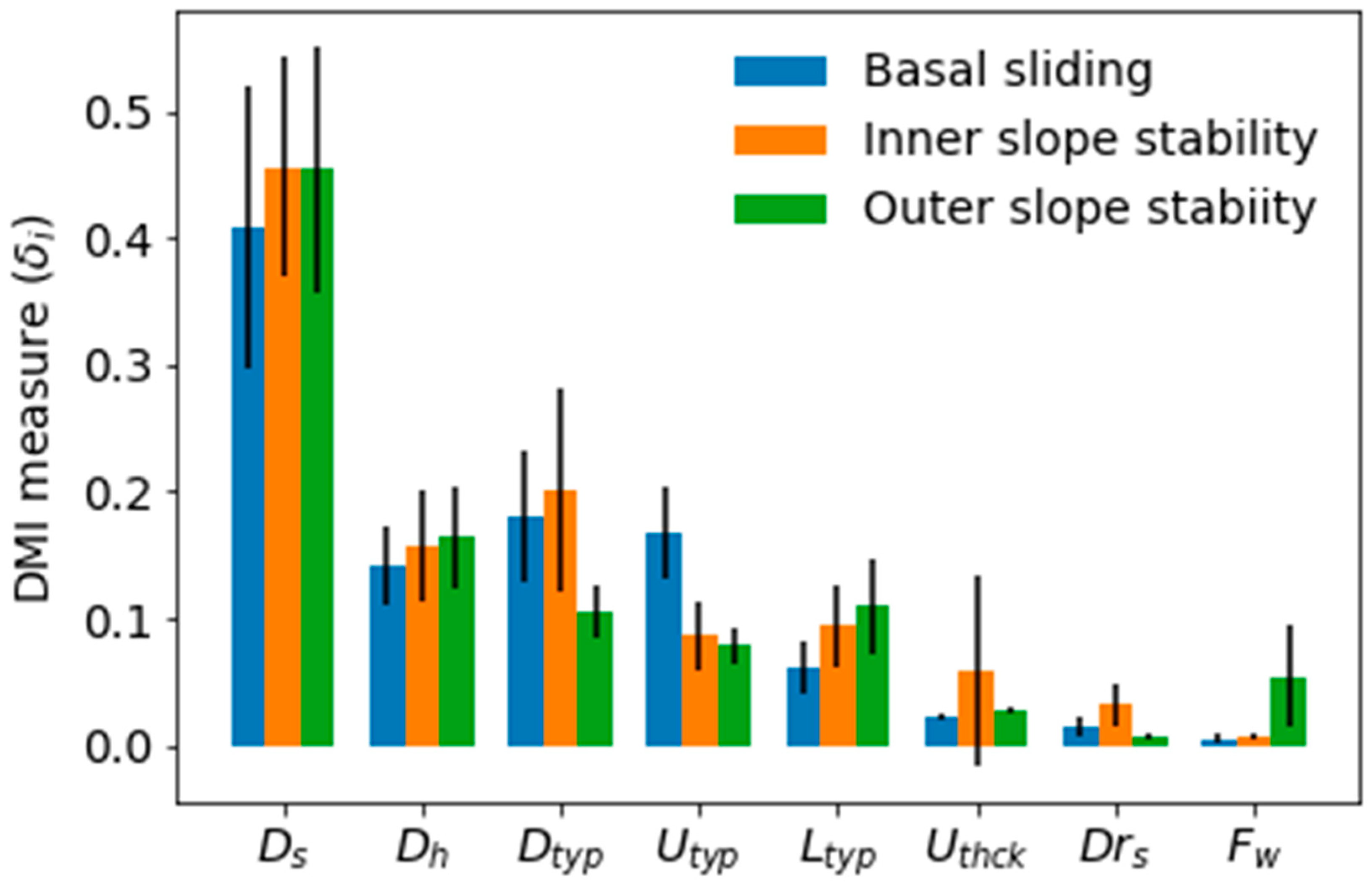
The eight sensitive parameters are selected for the global sensitivity analysis, which results in 390,625 combinations for each failure mechanism. The DMI method (Figure 7), based on differences in output probability density functions, clearly indicates that for each mechanism, the dike slope () is most influential. The other dike parameters, namely its height () and material properties (), are also among the more important factors. Furthermore, some input factors have a different importance for the different failure mechanisms. For example, the foreland width mainly influences the outer slope stability, while the spacing of drainage () mainly influences the inner slope. Other important differences include the relatively high influence of the for basal sliding, as the sliding surface at the dike base is in continuous contact with this upper subsurface layer. Two remarkable differences are the smaller influence of on outer slope stability, and the high standard deviation related to upper layer thickness regarding the inner slope stability (Figure 7). While these results indicate the importance of several input parameters, they do not provide further information about their relation to dike failure and local variability.
3.3. Trend Identification
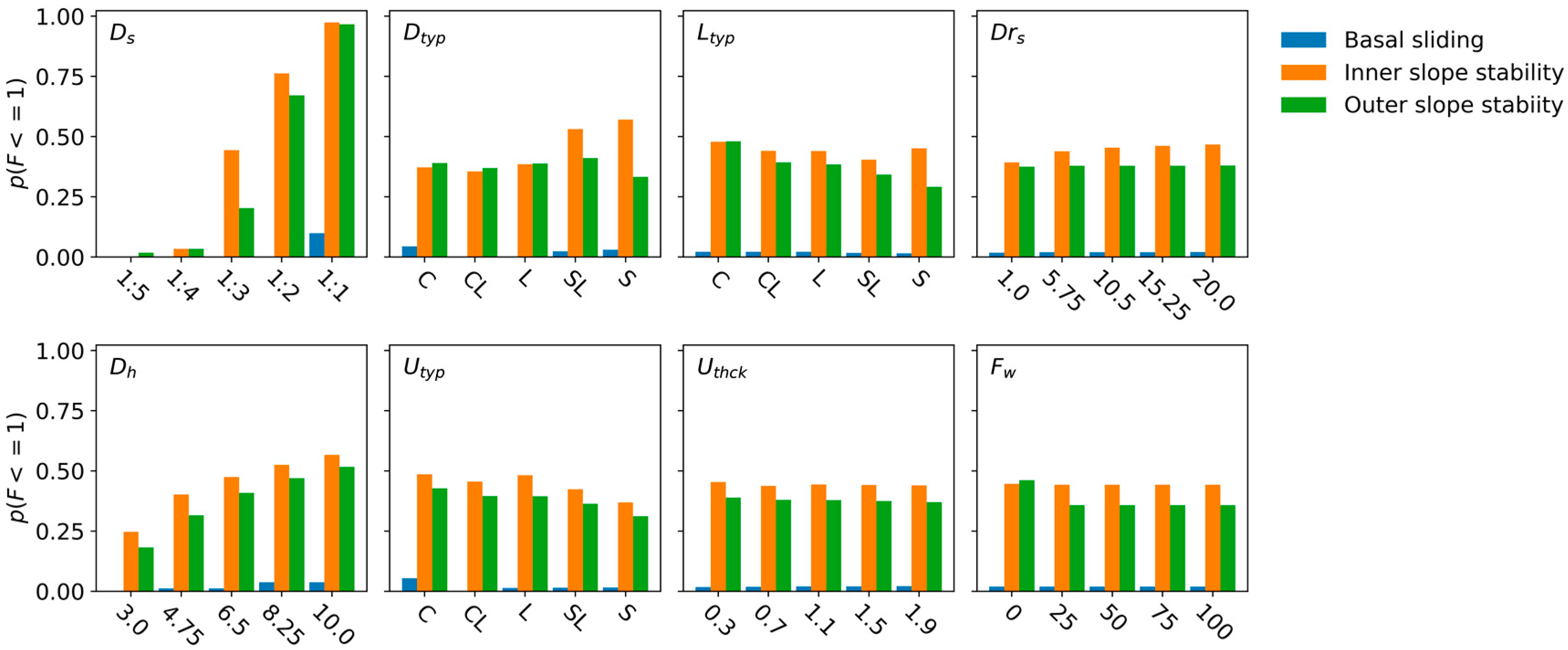
To identify the trend, the probability of an unstable dike given a certain input factor value is determined (Figure 8). For basal sliding, only a small fraction of the input factors’ combinations result in unstable dikes, making it the least important process of dike failure. For inner and outer slope stability, the effect is often similar, although critical safety factors are more often found for inner slope stability. Figure 8 reflects many of the DMI results (Figure 7), for example, a large influence of dike slope and dike height, where less steep sleep slopes and lower dikes are, in general, more likely to remain stable, and the small influence of . However, new insights become apparent too, as it is shown that an increase in foreland width () increases the outer slope stability only if the dike is less than 25 m away from the river. A similar effect is seen regarding drainage spacing (), which mostly decreases the inner slope stability at small distances from the dike (<10 m). The most important local variability, however, is observed for the material types, where a unidirectional change in the input factor does not necessarily result in a unidirectional change in dike stability. Where any shift towards a sandier subsurface will, on average, still result in a smaller for outer slope stability, this is not the case inner slope stability, which has its lowest at sandy loam. An even more striking trend is observed for , where the lowest failure probability for outer slope stability and the highest failure probability for inner slope stability both coincide at a sand dike. Although basal sliding results in failure less often, a similar local variability in the response can be observed.
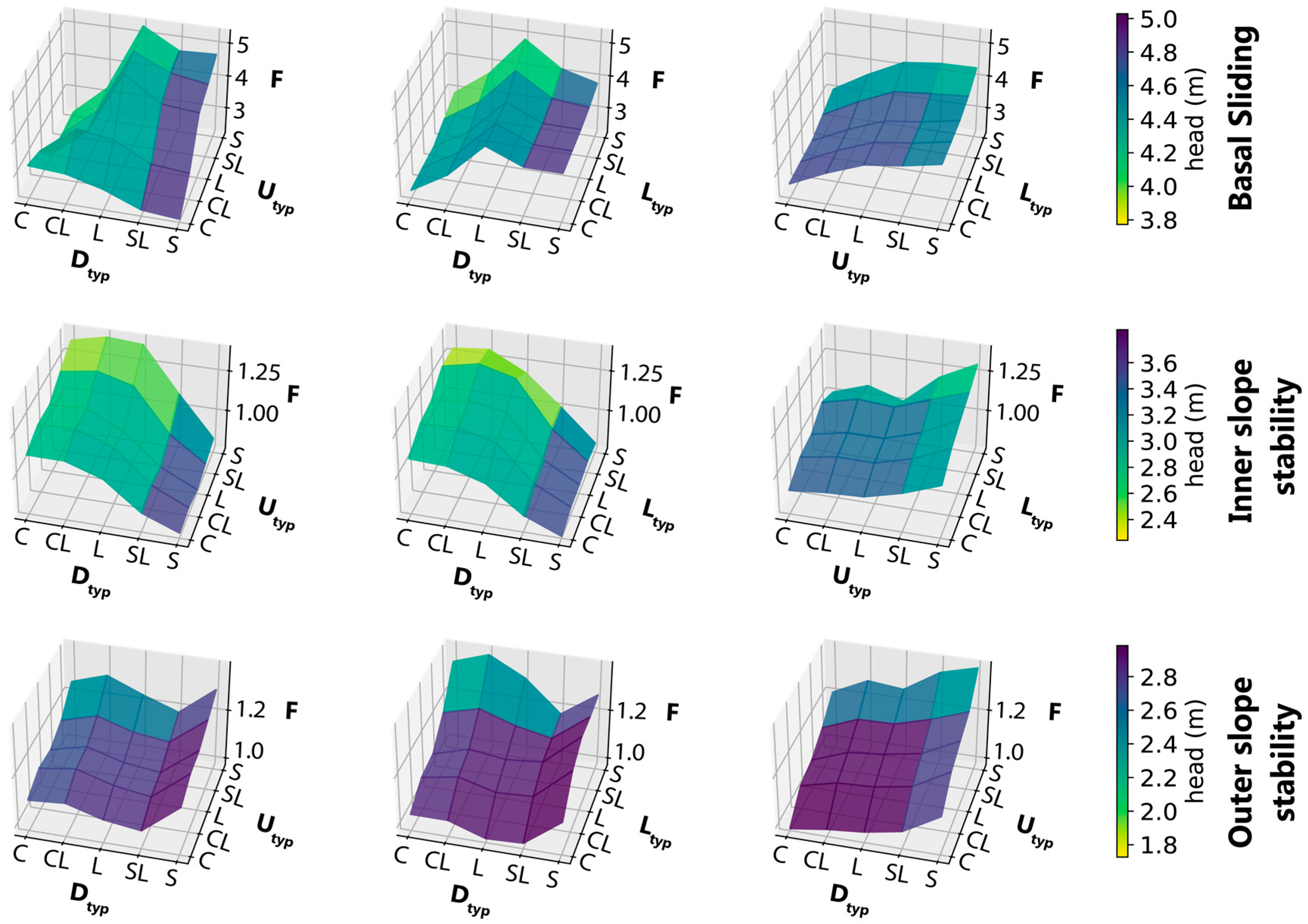
3.4. Subsurface Interaction Qualification
To explain these results in more detail, the response surfaces of the average dike stability at a given combination of material properties is compared with the corresponding pore pressure (Figure 9). The results are in line with the , which, for example, shows that sand as results in a low for inner slope stability, but reaches a high for outer slope stability (Figure 9). The results also show that low stability is strongly linked to high pore pressures, in addition to material parameters related to strength, such as cohesion or friction angle. This is mostly the case for basal sliding, where the low factors of safety are reached at both a clay dike/sand cover layer and a sand dike/clay cover, while high pore pressures are only observed in the latter situation.
However, for inner slope stability, there is a clear coincidence of high pore pressures, sand dikes and low values. As shown in Figure 5, the dikes are least stable at , which, due to the initial steady state, shows maximum groundwater heads for a dike type of sand, as it is more permeable. Sand dikes generally have low cohesion and rely largely on the frictional strength, but friction is lost as the high pore pressures reduce the effective normal stress. As the largest part of the slip surfaces intersects the dike and only slightly touches the cover layer, subsurface types and only have a minor influence on the dike’s stability on the inside.
This is not the case for outer slope stability, which often finds its most unstable condition at the end of river water drawdown. In this case, the dike’s stability is mostly dependent on the hydrological conditions, as lower stability coincides with higher pore pressures. Strikingly, low stability occurs most often for sandy loam, for which conductivity is high enough to become fully saturated during prolonged high river water levels, but low enough to prevent rapid drainage when the river level falls. This effect becomes more prominent when the material of the dike is more permeable than that of the underlying layers; therefore, the excess pore pressure during river level drawdown cannot dissipate to the underlying layers.
There are no apparent differences between shallow and deeper subsurface layers, although the explanation differs. In case of a shallow subsurface layer (), the lower permeability directly inhibits drainage into this layer, while an impermeable deeper subsurface layer () inhibits flow to the lateral drainage channels installed behind the dike.
4. Discussion and Practical Application
4.1. Global Sensitivity Indices for Groundwater Induced Dike Failure
Using the relations derived from the MC simulations, a database is constructed including the input factors and related factor of safety. For each failure mechanism, 390,625 parameter combinations are in this database, of which was 0.02, 0.443 and 0.379 for basal sliding, inner slope stability and outer slope stability, respectively. It follows that our assumptions of an infinitely long period of high-water level at the dike crest followed by a rapid drawdown both favor inner and outer slope failure. Nonetheless, the inner slope is generally more unstable, as its minimum stability is reached during the infinitely long high water, whereas outer slope failure only occurs during the drawdown. This rapid but transient drawdown decreases pore pressure, which thus increases friction and results in more stable conditions than on the inner slope. The larger fraction of simulations in the database with inner slope failures matches with practical experience [44], which suggests the modelling assumptions in this paper result in groundwater conditions that are representative of real-world conditions. Combining all the three mechanisms results in a total of 0.48 out of all the combinations, i.e., based on simulations that result in for one or more mechanisms.
All the parameters involved in the analysis have at least a small effect on the dike stability. In general, the least influential parameters are , and . However, the foreland width becomes influential at small values (Figure 8). Furthermore, the inner and outer slope stability are insensitive for changes in the dike width given the steady-state groundwater conditions, while the dike width does affects basal sliding. In addition, drainage spacing influences inner slope stability mainly if drainage occurs close to the dike. As such, many parameters have a considerable effect on a part of their parameter space and a given failure mechanism, but few are important over their entire parameter space and for all the failure mechanisms. This suggests that although global sensitivity analysis is a useful tool in determining the importance of parameters, the resulting sensitivity indices should be handled with care. In some cases, sensitivity indices such as the DMI [29] underestimate the general importance of a parameter, as they provide a mean parameter sensitivity that does not necessarily reflect the abundance of strong local effects.
4.2. Toward Flooding
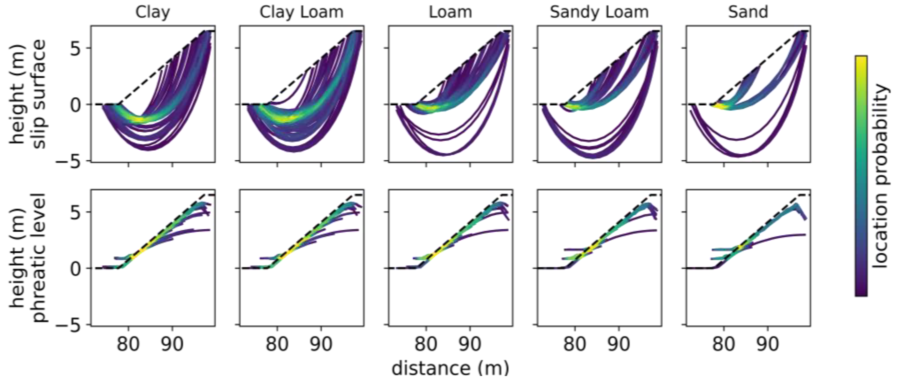
The probability of flooding is not only related to the probability of dike instability, but also to the water levels at the time of failure and the volume of the instability. To analyze the occurrence of these properties, we select the set of model runs for dikes with a 1:3 slope, a height of 6.5 m and a cover layer thickness of 1.5 m. Of the 625 selected scenarios that remain in the database with these parameters fixed, the slip surface shape and phreatic water level are related to the upper substrate type () for outer slope stability (Figure 10). In this example set, the area of failure decreases from 59.2 to 26.4 m2, while the mean phreatic level in the upper subsurface layer decreases from 2.36 to 1.93 m when the substrate material changes from clay to sand. Accordingly, the average safety factor increases from 1.06 to 1.29. This indicates not only that dike failure as a result of macro-instability is less likely due to occur with a sand subsurface, but also that potential instabilities are less threatening for a dike breach, as their volume is much smaller.
It should be noted that the groundwater model assumes a stationary response to the flood wave at the dike crest, but a transient response on the drawdown of this flood wave. From a hydrological perspective, the simulations thus start at a situation of minimal internal strength and, hence, minimal dike stability. However, as the high river water levels act as a stabilizing external force on the outer slope, this aspect of failure generally occurs after river water level drawdown. The breaches that subsequently occur create vulnerable dikes but, owing to the falling flood water levels, this is unlikely to lead to major dike beaches and flooding. Obviously, if this instability is followed by a second flood wave, the situation might become critical. Thus, additional research is needed in the transient dike response under very common multi-peak flood waves [45].
4.3. Limitations Regarding Sampling, Hydrology and Subsurface Uncertainty
First, this research used a uniform sampling strategy, not taking into account any possible correlations. We suggest, however, that by sampling each parameter uniformly over a range of possible outcomes and not taking account of possible but unknown correlations between parameters, we are likely to overestimate the possible range of outcomes. This conservative estimate of possibilities is deemed a rational choice, if no information is available about the a priori joint probability distribution of parameters.
Second, we used the most adverse hydrological conditions for dike slope stability calculations, being steady-state conditions for inner slope stability. We acknowledge that this might not be the case when considering flood duration and transient groundwater conditions, as the infiltration curve might not reach the inner toe and the safety factor becomes more favorable. A similar argument applies to basal sliding.
Third, this study used many possible scenarios of subsurface material and surface geometry combinations. Still, the subsurface material in this study is assumed to be homogeneous and deterministic in each of the layers, and likewise the layer thickness and surface profile are constant per section. Due to the long history and continuous improvement of many dikes, their interior is presumably very heterogeneous [6,7]. In reality, the subsurface properties, induced by previous river systems, are also known to have a large spatial variability [46,47]. These heterogeneous topographic and subsurface properties have a large influence on both hydrological conditions [48] and stability [49], while still ignoring the 3D slope effects [50]. In addition, animal burrows and human measures inhibiting or enhancing groundwater flow may also affect the pore pressure evolution.
4.4. Suggestions for Further Research
Nonetheless, the simulations show that for all the mechanisms, the dike type and upper layer type have a large effect on the dike stability. Despite their importance for dike stability and the valid assumption that they are heterogeneous, these two subsurface parameters are often partly unknown. As such, extending this research with variable material properties [11] may provide an even more extensive analysis of groundwater-related dike stability. In this way, the uncertainty of the material properties can be assessed too, which is important in real-world cases.
In addition to assessing the uncertainty, decreasing it is of major importance when assessing dike stability [51]; this is achieved by having more detailed subsurface data available. Thus, incorporating large scale subsurface heterogeneity (in 3D) is an important step in actively incorporating groundwater calculations in dike stability calculations, although we are confident that the large contrast in dike and subsurface materials used in this study, to a great extent, covers the large variation across many dikes.
Furthermore, additional research is needed in the transient groundwater response given a certain flood wave instead of steady-state conditions. Finally, the database constructed and explored in this paper could be used for mapping those regions where factors of safety might reach critical values.
4.5. Case Study: Application of the Database for Fast High-Resolution Dike Safety Assessment
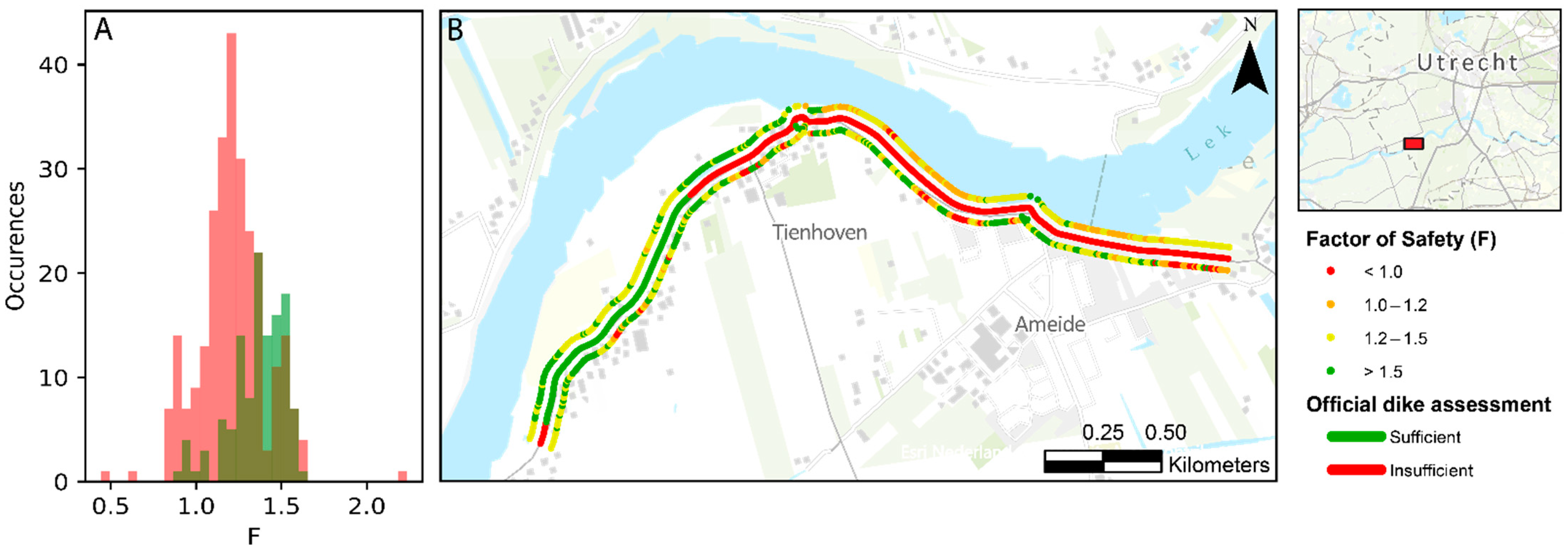
As a first attempt for identifying those regions, the created database was applied to a real-world case. This case concerns the area near the village of Ameide in The Netherlands (51.954594 N, 4.963298 E; Figure 11), for which an official preliminary assessment of the dike stability was made [52]. The failure probability of the dike was calculated using the Bishop’s modified method [53], and based on the characteristic values of material strength parameters. The phreatic level was simplified in the schematization and was roughly a straight line between the river water level and the ditch water level. In the assessment, larger segments with reasonably similar characteristics were tested against a failure probability of 1/360 years and assigned the final judgement. In a later stage, the precision of these judgements was drastically improved using local schematizations and locally derived characteristics for the important parameters; hence, the current assessment was seen as preliminary.
4.5.1. Case Study Methodology
The dike in this area was subdivided in segments with a length of 100 m, of which several failed to meet the expected failure probability. Here, we compared the values of the factor of safety for comparable situations in terms of dike geometry and composition from the Monte Carlo simulations with the assessment in order to test whether unsafe conditions were revealed by our approach. We hypothesized that using a pre-constructed database with factors of safety in combination with actual dike characteristics could provide a quick a priori analysis of the dike stability. To compare the official assessment with the database, those dike parameters should be selected from a database that corresponds to the actual dike. The parameters concerning geometry and composition of the dike and the subsurface were determined at an interval of 10 m along the entire dike crest. The dike height, crest width and slope were automatically derived from the high-resolution lidar-based AHN3 surface elevation model. The properties of the subsurface, being layer thickness and lithology, were derived from the GeoTOP subsurface model [54]. An approximation of the dike material was made from publicly available cone penetration tests (BRO) using a simple but effective method proposed by [55]. When these parameters were assembled, the corresponding safety factor was selected from the database.
4.5.2. Case Study Results
First, as the acquisition of surface geometry and subsurface composition can have a high spatial resolution of 10 m, it provides more detailed information than the official assessment, which is conducted on a 100-meter resolution. On visual inspection, the calculated safety factors already clearly coincide with the official dike assessment (Figure 11B), although the variation of the calculated values is much higher, as the official safety assessments are carried out only per 100 m section, whereas the factor of safety is calculated here every 10 m. There is also a clear difference visible between the inner and outer slope stability. Those dike sections that are assessed as sufficiently safe have an average safety factor of 1.53 ± 0.31 and 1.44 ± 0.13 for their inner and outer slope stability, respectively. The insufficiently safe sections according to the official assessment have a calculated average safety factor of 1.41 ± 0.38 and 1.34 ± 0.20, respectively. Thus, according to our method, most of the sections found to be insufficiently safe have an F 1 (Figure 11A). In the official assessment, 69.3% of the dike was found insufficiently safe against 10.8% in our analysis. Of this 10.8%, 9.5% is found on the insufficiently safe sections and 1.3% is found on those sections that were found to be safe enough.
4.5.3. Case Study Discussion and Conclusions
These false positive assessments, all occurring on the inner dike slope, are most dangerous. Their lower safety factors are caused by a combination of steeper dike slopes and the presence of sandy dike material. Thus, in addition to showing high spatial variability in the expected factor of safety, the analysis also clearly shows those sections that, according to our calculations, are the most critical. These differences seem to be largely related to variations in dike material but can also be related to some of the parameters (drainage, dynamic river level) that are not included in our analysis. Moreover, it is likely the cause of different definitions of failure and the use of different stability calculation methods, such as drained or undrained loading [39]. In conclusion, the high-resolution database comparison could help to focus further research and data assembly, by indicating areas to improve local schematizations and derive local characteristics for the important parameters in a more detailed stage of dike reinforcement design.
5. Conclusions
In this study, an extensive global sensitivity analysis was carried out for dike stability using calculated groundwater heads and resulting pore pressures that represent a worst-case scenario. The following three sensitivity settings formed the basis of this analysis: parameter prioritization, trend identification and interaction qualification. The results show that each of the three studied failure mechanisms, namely, basal sliding, inner slope stability and outer slope stability, can possibly result in dike failure, where failure on the inner slope of the dike is the most likely.
In the parameter prioritization settings, eight parameters were determined to be influential for any of the failure mechanisms, being dike slope, dike height, dike material type, upper layer material type, lower layer material type, upper layer thickness, drainage spacing and foreland width. In contrast, the dike crest width, drainage depth and aquifer thickness had a negligible effect on the stability. According to the Delta Moment-Independent measure (Equation (4)), the dike slope was found to have the largest effect on dike stability, as it has both a direct effect on slope stability (Figure 5) and indirectly affects the slope stability by changing the pore pressure conditions (Figure 7). We conclude that the delta sensitivity index provides a clear indication of parameter importance. The Delta Moment-Independent measure does not provide information on parameter interaction and the underlying mechanisms.
A regional sensitivity analysis by means of the probability of failure was used to show local and process dependent variability. This measure shows that dike slope and dike material are most influential for resulting in unstable dikes. Furthermore, it indicates local variability, such as that drainage spacing only affects the inner slope stability if the drainage location is close to the dike. Combining the Delta Moment-Independent measure indices and the showed that while basal sliding is most sensitive to changes in most parameters, it is least likely to result in dike failure.
In addition, we qualified the interaction between different material types, hydrology and stability. Most strikingly, a combination of a relatively permeable dike and impermeable subsurface inhibits the dissipation of pore pressures to the lower layers. Therefore, pore pressures remain high and dike instabilities are more likely to occur. This effect is more prominent for outer slope stability, as dissipating high pore pressures is mostly important during river level drawdown. The area of failure is often also larger in case of an impermeable subsurface, increasing the chance of severe flooding after a slope instability.
Applying the database containing geometry parameters, subsurface properties and safety factors to a real case resulted in high-resolution estimates of dike stability. These estimates show that the unsafe segments derived from the database are mostly on those segments also found to be unsafe by the official assessment, although there are some false positives, e.g., segments that are estimated to be unsafe but classified as safe in the assessment. Overall, the database estimates provide a more differentiated picture and allows for more targeted analyses and measures. Although three-dimensional subsurface buildup and variable flood waves can improve the simulation results, the comparison gives confidence that our results provide useful insights in the process of groundwater-related dike stability and that the underlying database can be used to focus additional local research. The analysis of groundwater-related dike failure with global sensitivity methods clearly shows the importance of high-resolution groundwater modelling for estimating dike slope stability.
Author Contributions
T.v.W., R.v.B., M.F.P.B. and H.M. designed the research. T.v.W. and R.v.B. performed the primary data analysis and model development. H.M. and M.F.P.B. helped with result interpretation. All authors have read and agreed to the published version of the manuscript.
Funding
This project was supported by funding from the Netherlands Organisation for Scientific Research (NWO-TTW) within the All-Risk project (grant No. P15-21).
Institutional Review Board Statement
Not applicable.
Informed Consent Statement
Not applicable.
Data Availability Statement
A dataset containing the results and input parameters for the Monte Carlo analysis can be found online [56].
Acknowledgments
We greatly appreciated the support of Edwin Sutanudjaja and Lukas van de Wiel providing the computational power needed for the Monte Carlo simulations.
Conflicts of Interest
The authors declare no conflict of interest. The funders had no role in the design of the study; in the collection, analyses, or interpretation of data; in the writing of the manuscript, or in the decision to publish the results.
References
- Tourment, R. European and US Levees and Flood Devences; Characteristics, Risks and Governance. 2018. Available online: www.barrages-cfbr.eu (accessed on 2 December 2019).
- ICOLD. Twenty-Sixth International Congress on Large Dams/Vingt-Sixieme Congrès des Grands Barrages, Vienna, Austria, 4–6 July, 2018, 1st ed.; CRC Press: London, UK, 2018; p. 300. [Google Scholar]
- IPCC. Summary for Policymakers. Contribution of Working Group III to the Fifth Assessment Report of the Intergovernmental Panel on Climate Change. In Climate Change 2014: Mitigation of Climate Change; Edenhofer, O.R., Pichs-Madruga, Y., Sokona, E., Farahani, S., Kadner, K., Seyboth, A., Adler, I., Baum, S., Brunner, P., Eickemeier, B., et al., Eds.; Cambridge University Press: Cambridge, UK; New York, NY, USA, 2014. [Google Scholar] [CrossRef] [Green Version]
- Middelkoop, H.; Daamen, K.; Gellens, D.; Grabs, W.; Kwadijk, J.; Lang, H.; Parmet, B.W.A.H.; Schädler, B.; Schulla, J.; Wilke, K. Impact of climate change on hydrological regimes and water resources management in the Rhine Basin. Clim. Chang. 2001, 49, 105–128. [Google Scholar] [CrossRef]
- Eijgenraam, C.; Kind, J.; Bak, C.; Brekelmans, R.; Hertog, D.D.; Duits, M.; Roos, K.; Vermeer, P.; Kuijken, W. Economically efficient standards to protect the Netherlands against flooding. Interfaces 2014, 44, 7–21. [Google Scholar] [CrossRef] [Green Version]
- Meehan, C.L.; Benjasupattananan, S. An analytical approach for levee underseepage analysis. J. Hydrol. 2012, 470, 201–211. [Google Scholar] [CrossRef] [Green Version]
- Polanco, L.; Rice, J. A reliability-based evaluation of the effects of geometry on levee underseepage potential. Geotech. Geol. Eng. 2014, 32, 807–820. [Google Scholar] [CrossRef]
- Stanisz, J.; Borecka, A.; Pilecki, Z.; Kaczmarczyk, R. Numerical simulation of pore pressure changes in levee under flood conditions. E3S Web Conf. 2017, 24, 3002. [Google Scholar] [CrossRef] [Green Version]
- Mateo-Lázaro, J.; Sánchez-Navarro, J..; García-Gil, A.; Edo-Romero, V.; Castillo-Mateo, J. Modelling and layout of drainage-levee devices in river sections. Eng. Geol. 2016, 214, 11–19. [Google Scholar] [CrossRef]
- Peñuela, W.F. River Dyke Failure Modeling under Transient Water Conditions; ETH-Zürich: Zürich, Switzerland, 2013. [Google Scholar]
- Lanzafame, R.; Teng, H.; Sitar, N. Stochastic analysis of levee stability subject to variable seepage conditions. Geo-Risk 2017, 554–563. [Google Scholar] [CrossRef] [Green Version]
- Vahedifard, F.; Sehat, S.; Aanstoos, J.V. Effects of rainfall, geomorphological and geometrical variables on vulnerability of the lower Mississippi River levee system to slump slides. Georisk Assess. Manag. Risk Eng. Syst. Geohazards 2017, 11, 257–271. [Google Scholar] [CrossRef]
- Canli, E.; Mergili, M.; Thiebes, B.; Glade, T. Probabilistic landslide ensemble prediction systems: Lessons to be learned from hydrology. Nat. Hazards Earth Syst. Sci. 2018, 18, 2183–2202. [Google Scholar] [CrossRef] [Green Version]
- Collison, A.J.C.; Anderson, M.G. Using a combined slope hydrology/stability model to identify suitable conditions for landslide prevention by vegetation in the humid tropics. Earth Surf. Process. Landf. 1996, 21, 737–747. [Google Scholar] [CrossRef]
- Malet, J.-P.; Van Asch, T.W.J.; Van Beek, R.; Maquaire, O. Forecasting the behaviour of complex landslides with a spatially distributed hydrological model. Nat. Hazards Earth Syst. Sci. 2005, 5, 71–85. [Google Scholar] [CrossRef] [Green Version]
- Iooss, B.; Lemaître, P.A. A review on global sensitivity analysis methods. Oper. Res. Comput. Sci. Interfaces Ser. 2015, 59, 101–122. [Google Scholar] [CrossRef] [Green Version]
- Saltelli, A.; Ratto, M.; Andres, T.; Campolongo, F.; Cariboni, J.; Gatelli, D.; Saisana, M.; Tarantola, S. Global Sensitivity Analysis. The Primer; John Wiley & Sons: Hoboken, NJ, USA, 2008. [Google Scholar]
- Ferretti, F.; Saltelli, A.; Tarantola, S. Trends in sensitivity analysis practice in the last decade. Sci. Total Environ. 2016, 568, 666–670. [Google Scholar] [CrossRef]
- Pianosi, F.; Beven, K.; Freer, J.; Hall, J.W.; Rougier, J.; Stephenson, D.B.; Wagener, T. Sensitivity analysis of environmental models: A systematic review with practical workflow. Environ. Model. Softw. 2016, 79, 214–232. [Google Scholar] [CrossRef]
- Song, X.; Zhang, J.; Zhan, C.; Xuan, Y.; Ye, M.; Xu, C. Global sensitivity analysis in hydrological modeling: Review of concepts, methods, theoretical framework, and applications. J. Hydrol. 2015, 523, 739–757. [Google Scholar] [CrossRef] [Green Version]
- Borgonovo, E.; Lu, X.; Plischke, E.; Rakovec, O.; Hill, M.C. Making the most out of a hydrological model data set: Sensitivity analyses to open the model black-box. Water Resour. Res. 2017, 53, 7933–7950. [Google Scholar] [CrossRef]
- Ciriello, V.; Lauriola, I.; Tartakovsky, D.M. Distribution-based global sensitivity analysis in hydrology. Water Resour. Res. 2019, 55, 8708–8720. [Google Scholar] [CrossRef]
- Ratto, M.; Young, P.C.; Romanowicz, R.; Pappenberger, F.; Saltelli, A.; Pagano, A. Uncertainty, sensitivity analysis and the role of data based mechanistic modeling in hydrology. Hydrol. Earth Syst. Sci. 2007, 11, 1249–1266. [Google Scholar] [CrossRef] [Green Version]
- Janetti, E.B.; Guadagnini, L.; Riva, M.; Guadagnini, A. Global sensitivity analyses of multiple conceptual models with uncertain parameters driving groundwater flow in a regional-scale sedimentary aquifer. J. Hydrol. 2019, 574, 544–556. [Google Scholar] [CrossRef]
- Guo, X.; Dias, D.; Pan, Q. Probabilistic stability analysis of an embankment dam considering soil spatial variability. Comput. Geotech. 2019, 113, 103093. [Google Scholar] [CrossRef]
- Hamm, N.; Hall, J.; Anderson, M. Variance-based sensitivity analysis of the probability of hydrologically induced slope instability. Comput. Geosci. 2006, 32, 803–817. [Google Scholar] [CrossRef]
- Xu, Z.; Zhou, X.; Qian, Q. The uncertainty importance measure of slope stability based on the moment-independent method. Stoch. Environ. Res. Risk Assess. 2020, 34, 51–65. [Google Scholar] [CrossRef]
- Morris, M.D. Factorial sampling plans for preliminary computational experiments. Technometrics 1991, 33, 161–174. [Google Scholar] [CrossRef]
- Borgonovo, E. A new uncertainty importance measure. Reliab. Eng. Syst. Saf. 2007, 92, 771–784. [Google Scholar] [CrossRef]
- Hughes, J.D.; Langevin, C.D.; Banta, E. Documentation for the MODFLOW 6 Framework; U.S. Geological Survey: Reston, VA, USA, 2017. [CrossRef]
- Langevin, C.D.; Hughes, J.D.; Banta, E.; Provost, A.; Niswonger, R.; Panday, S. MODFLOW 6, the U.S. Geological Survey Modular Hydrologic Model; Version 6.1.1; USGS: Reston, VA, USA, 2019. [CrossRef]
- Fredlund, D.G.; Krahn, J.; Pufahl, D.E. The relationship between limit equilibrium slope stability methods. In Soil Mechanics and Foundation Engineering, Proceedings of the 10th International Conference, Stockholm, Sweden, 15–19 June 1981; Balkema, A.A., Ed.; Publ. Rotterdam: Rotterdam, The Netherlands, 1981; Volume 3, pp. 409–416. [Google Scholar] [CrossRef]
- Fredlund, D.G.; Krahn, J. Comparison of slope stability methods of analysis. Can. Geotech. J. 1977, 14, 429–439. [Google Scholar] [CrossRef]
- Morgenstern, N.R.; Price, V.E. The analysis of the stability of general slip surfaces. Geotechnique 1965, 15, 79–93. [Google Scholar] [CrossRef]
- Malkawi, A.H.; Hassan, W.F.; Sarma, S.K. An efficient search method for finding the critical circular slip surface using the Monte Carlo technique. Can. Geotech. J. 2001, 38, 1081–1089. [Google Scholar] [CrossRef]
- Campolongo, F.; Cariboni, J.; Saltelli, A. An effective screening design for sensitivity analysis of large models. Environ. Model. Softw. 2007, 22, 1509–1518. [Google Scholar] [CrossRef]
- Pachepsky, Y.; Park, Y. Saturated hydraulic conductivity of us soils grouped according to textural class and bulk density. Soil Sci. Soc. Am. J. 2015, 79, 1094–1100. [Google Scholar] [CrossRef]
- CEN. Eurocode 7: Geotechnical Design—Part 1: General Rules; European Committee for Standardisation: Brussels, Belgium, 2004; p. 171. [Google Scholar]
- Conklin, H.E. Soil Survey Manual, 3rd ed.; USDA, Government Printing Office: Washington, DC, USA, 1952; Volume 34.
- Andres, T. Sampling methods and sensitivity analysis for large parameter sets. J. Stat. Comput. Simul. 1997, 57, 77–110. [Google Scholar] [CrossRef]
- Nossent, J.; Elsen, P.; Bauwens, W. Sobol’ sensitivity analysis of a complex environmental model. Environ. Model. Softw. 2011, 26, 1515–1525. [Google Scholar] [CrossRef]
- Tang, Y.; Reed, P.; Van Werkhoven, K.; Wagener, T. Advancing the identification and evaluation of distributed rainfall-runoff models using global sensitivity analysis. Water Resour. Res. 2007, 43. [Google Scholar] [CrossRef]
- Powell, M.J.D. An efficient method for finding the minimum of a function of several variables without calculating derivatives. Comput. J. 1964, 7, 155–162. [Google Scholar] [CrossRef]
- Stuij, S.; de Wit, T.; Huting, R. Dijkversterking Grebbedijk; Royal Haskoning DHV: Amersfoort, The Netherlands, 2017. [Google Scholar]
- Hegnauer, M.; Beersma, J.J.; van den Boogaard, H.F.P.; Buishand, T.A.; Passchier, R.H. Generator of Rainfall and Discharge Extremes (GRADE) for the Rhine and Meuse Basins. Final Report of GRADE 2.0. 2014. Available online: http://projects.knmi.nl/publications/fulltexts/1209424004zws0018rgenerator_of_rainfall_and_discharge_extremes_grade_for_the_rhine_and_meuse_basins_definitief.pdf (accessed on 20 September 2018).
- Berendsen, H.J.; Stouthamer, E. Late Weichselian and Holocene palaeogeography of the Rhine–Meuse Delta, The Netherlands. Palaeogeogr. Palaeoclim. Palaeoecol. 2000, 161, 311–335. [Google Scholar] [CrossRef]
- Bierkens, M.F. Modeling hydraulic conductivity of a complex confining layer at various spatial scales. Water Resour. Res. 1996, 32, 2369–2382. [Google Scholar] [CrossRef]
- Wang, X.; Wang, H.; Liang, R.Y. A method for slope stability analysis considering subsurface stratigraphic uncertainty. Landslides 2017, 15, 925–936. [Google Scholar] [CrossRef]
- Hicks, M.; Nuttall, J.; Chen, J. Influence of heterogeneity on 3D slope reliability and failure consequence. Comput. Geotech. 2014, 61, 198–208. [Google Scholar] [CrossRef]
- Gong, W.; Tang, H.; Wang, H.; Wang, X.; Juang, C.H. Probabilistic analysis and design of stabilizing piles in slope considering stratigraphic uncertainty. Eng. Geol. 2019, 259, 105162. [Google Scholar] [CrossRef]
- Deltacommissie. Samen Werken Met Water. Een Land Dat Leeft, Bouwt aan Zijn Toekomst. Bevindingen van de Deltacommissie 2008. Available online: http://www.deltacommissie.com/doc/2008-09-03AdviesDeltacommissie.pdf%0Ahttp://scholar.google.com/scholar?hl=en&btnG=Search&q=intitle:Samen+werken+met+water#1 (accessed on 9 October 2018).
- Consortium DOT. Veiligheid Nederland in Kaart 2, Overstromingsrisico Dijkring 16 Alblasserwaard en de Vijfheerenlanden; Royal Haskoning DHV: Amersfoort, The Netherlands, 2014. [Google Scholar]
- Bishop, A.W. The use of the slip circle in the stability analysis of slopes. Geotechnique 1955, 5, 7–17. [Google Scholar] [CrossRef]
- Stafleu, J.; Dubelaar, C.W. Product Specification—Subsurface Model GeoTOP (TNO 2016 R10133 | 1.3). 2016. Available online: www.tno.nl (accessed on 20 September 2018).
- Begemann, H.K. The friction jacket cone as an aid in determining the soil profile. In Proceedings of the 6th International Conference on Soil Mechanics and Foundation Engineering, Christchurch, New Zealand; Montréal, QC, Canada, 8–15 September 1965; Volume 1, pp. 17–20. [Google Scholar]
- van Woerkom, T.A.A. Monte-Carlo simulation of dike stability based on a coupled steady-state hydro-stability model. Zenodo 2020. [Google Scholar] [CrossRef]
Figure 1.
Schematization of model inputs, indicating the setup of the hydrological model. See for their meaning, values and possible ranges Table 1 and Table 2.

Figure 2.
Workflow of Global Sensitivity Analysis, focusing on the pre-processing by factor fixing and performing the model runs. The specific measures used to qualify and quantify sensitivity are discussed in Figure 4.
Figure 2.
Workflow of Global Sensitivity Analysis, focusing on the pre-processing by factor fixing and performing the model runs. The specific measures used to qualify and quantify sensitivity are discussed in Figure 4.

Figure 3.
Subsurface types used in the analysis as seen in the soil textural triangle, modified from [39].
Figure 3.
Subsurface types used in the analysis as seen in the soil textural triangle, modified from [39].

Figure 4.
Visual explanation of both SA methods used. The elementary effect (A) uses a fixed step (, equation 3) of input factor from a random starting points and measures the change in result . Note that all arrows are of the same size in the X direction, representing the fixed step size. The DMI method (B) is based on the area difference (highlighted in red) between the continuous unconditional probability density function and a conditional unconditional probability density function , which is based on a sample of the unconditional input vector.

Figure 5.
Example results of the coupled hydro-stability model. Left two columns: steady state with maximum loading equal to dike crest. Right two columns: falling water levels from dike crest to dike toe. Continuous colored lines indicate hydraulic heads at the depth of the dotted lines with a corresponding color. The black curved lines indicate the sliding planes on the inner and outer slope of the dike associated with the minimal safety factor. indicates the steady-state results at maximum pressure, and shows the results with water levels returned to the dike toe elevation. For each situation the safety factors of basal sliding ( ), inner slope stability ( ) and outer slope stability () are presented.

Figure 6.
Factor Elementary Effects, leading to the factor rank per failure mechanism (A). Fixing the insensitive factors results in the final scatter plot between the results of the unconditional (unfixed) input, and conditional (partly fixed) input (B), leading to a combined of 0.985. Eight parameters (selection x-axis) are selected for the Monte-Carlo analysis, namely dike slope ( ), dike height ( ), dike material type ( ), upper layer material type ( ), lower layer material type ( ), upper layer thickness ( ), drainage spacing ( ) and foreland width ( ).

Figure 7.
Results of global sensitivity analysis (DMI-method). The bars indicate the Delta Moment-Independent measure ( per failure mechanism where higher values indicate a greater sensitivity of the factor of safety to that variable (Table 1). Error bars show the values 1 standard deviation (1 ). Wider error bounds indicate greater variance in the sensitivity for that parameter, possibly caused by parameter interaction.

Figure 8.
Probability of failure given that the selected input factor is fixed at the given value on the x-axis, and all other input factors are not fixed. Where equals 0 all calculated dikes are stable, and with a of 1, all calculated dikes fail. A large difference in the probability of failure between neighboring bars indicates a strong local importance of that factor.

Figure 9.
Response surfaces of dike stability on different combinations of dike and subsurface properties. Low factors of safety clearly coincide with high (darker blue) hydraulic heads for each failure mechanism. Note the different scales for both the y-axis ( ) as the colors (heads).
Figure 9.
Response surfaces of dike stability on different combinations of dike and subsurface properties. Low factors of safety clearly coincide with high (darker blue) hydraulic heads for each failure mechanism. Note the different scales for both the y-axis ( ) as the colors (heads).

Figure 10.
Probability of slip surface location and phreatic surface for different types of upper layer () material. Brighter colors indicate a larger probability of, respectively, the slip surfaces or phreatic surfaces to occur at that location.
Figure 10.
Probability of slip surface location and phreatic surface for different types of upper layer () material. Brighter colors indicate a larger probability of, respectively, the slip surfaces or phreatic surfaces to occur at that location.

Figure 11.
Comparison between official preliminary dike safety assessment and safety factors derived from our database. The histograms (A) of the safety factors corresponding to the sufficiently safe (green) or insufficiently safe (red) dike segments clearly show a clear distinction in our database between these segments. Spatially (B), both inner and outer slope stability show a much larger variation in safety factors than the official dike assessment suggests.


Table 1.
Name, symbol and range of the model parameters. A visualization of each of the parameters is shown in Figure 1. Layer type descriptions are found in Table 2.
| Parameter | Symbol | Range | Unit |
|---|---|---|---|
| Dike Height | 3–10 | m | |
| Dike crest width | 2–5 | m | |
| Dike slope | 0.2–1 | m/m | |
| Dike type | C-CL-L-SL-S | - | |
| Upper layer thickness | 0.3–1.9 | m | |
| Upper layer type | C-CL-L-SL-S | - | |
| Lower layer thickness | 5–10 | m | |
| Lower layer type | C-CL-L-SL-S | - | |
| Foreland width | 0–100 | m | |
| Drainage depth | 0.1–2 | m | |
| Drainage spacing | 1–20 | m | |
| Riverbed slope | 0.33 | m/m | |
| River depth | ) | m | |
| Flood height | m | ||
| Drawdown time | 1 | days |
Table 2.
Subsurface types used in the model, related to the , and parameters. The subsurface type is linked to the hydraulic conductivity ( ), drained cohesion ( ), effective friction angle ( ), the bulk unit weight ( ) and the saturated bulk unit weight ( ).
Table 2.
Subsurface types used in the model, related to the , and parameters. The subsurface type is linked to the hydraulic conductivity ( ), drained cohesion ( ), effective friction angle ( ), the bulk unit weight ( ) and the saturated bulk unit weight ( ).
| Subsurface Type | Abbreviation | |||||
|---|---|---|---|---|---|---|
| Clay | C | 0.13 | 5.0 | 17.5 | 17 | 17 |
| Clay-Loam | CL | 0.18 | 4.0 | 22.5 | 18 | 18 |
| Loam | L | 0.19 | 1.0 | 30.0 | 20 | 20 |
| Sandy Loam | SL | 1.54 | 0.5 | 31.25 | 19.5 | 19.5 |
| Sand | S | 8.94 | 0.0 | 32.5 | 18 | 20 |
Table 3.
Minimum per failure mechanism and parameter values of input vector X resulting in that minimum . See Table 1 for the abbreviations and units of the parameters.
Table 3.
Minimum per failure mechanism and parameter values of input vector X resulting in that minimum . See Table 1 for the abbreviations and units of the parameters.
| Basal sliding | 0.69 | 9.97 | 2.14 | 1:1 | Sand | 0.31 | Clay | 5.07 | Clay | 50 | −1.05 | 20.0 |
| Inner slope stability | 0.00 | 9.74 | 3.50 | 1:1 | Sand | 1.10 | Clay-Loam | 7.50 | Clay-Loam | 50 | −1.05 | 10.5 |
| Outer slope stability | 0.26 | 9.34 | 4.61 | 1:1 | Sandy Loam | 1.82 | Loam | 5.25 | Clay-Loam | 85 | −0.62 | 20.0 |
Publisher’s Note: MDPI stays neutral with regard to jurisdictional claims in published maps and institutional affiliations. |
© 2021 by the authors. Licensee MDPI, Basel, Switzerland. This article is an open access article distributed under the terms and conditions of the Creative Commons Attribution (CC BY) license (https://creativecommons.org/licenses/by/4.0/).
Share and Cite
MDPI and ACS Style
van Woerkom, T.; van Beek, R.; Middelkoop, H.; Bierkens, M.F.P. Global Sensitivity Analysis of Groundwater Related Dike Stability under Extreme Loading Conditions. Water 2021, 13, 3041. https://doi.org/10.3390/w13213041
AMA Style
van Woerkom T, van Beek R, Middelkoop H, Bierkens MFP. Global Sensitivity Analysis of Groundwater Related Dike Stability under Extreme Loading Conditions. Water. 2021; 13(21):3041. https://doi.org/10.3390/w13213041
Chicago/Turabian Stylevan Woerkom, Teun, Rens van Beek, Hans Middelkoop, and Marc F. P. Bierkens. 2021. "Global Sensitivity Analysis of Groundwater Related Dike Stability under Extreme Loading Conditions" Water 13, no. 21: 3041. https://doi.org/10.3390/w13213041
Note that from the first issue of 2016, this journal uses article numbers instead of page numbers. See further details here.