
Investigating Behavior of Six Methods for Sediment Transport Capacity Estimation of Spatial-Temporal Soil Erosion
by
 , , ,
, , ,
Linh Nguyen Van
1 ,
,
Xuan-Hien Le
2,3 ,
,
Giang V. Nguyen
1, 
Minho Yeon
1,
Sungho Jung
1 and
Giha Lee
1,* 1
Department of Advanced Science and Technology Convergence, Kyungpook National University, 2559 Gyeongsang-daero, Sangju 37224, Korea
2
Disaster Prevention Emergency Management Institute, Kyungpook National University, 2559 Gyeongsang-daero, Sangju 37224, Korea
3
Faculty of Water Resources Engineering, Thuyloi University, 175 Tay Son, Dong Da, Hanoi 100000, Vietnam
*
Author to whom correspondence should be addressed.
Water 2021, 13(21), 3054; https://doi.org/10.3390/w13213054
Submission received: 6 September 2021
/
Revised: 21 October 2021
/
Accepted: 29 October 2021
/
Published: 1 November 2021
(This article belongs to the Special Issue Research on Soil Erosion and Sediment Transport in Catchment)
Abstract
:Estimation of sediment transport capacity (STC) plays a crucial role in simulating soil erosion using any physics-based models. In this research, we aim to investigate the pros and cons of six popular STC methods (namely, Shear velocity, Kilinc-Richardson (KR), Effective stream power, Slope and unit discharge, Englund-Hansen (EH), and Unit stream power) for soil erosion/deposition simulation at watershed scales. An in-depth analysis was performed using the selected STC methods integrated into the Grid Surface Subsurface Hydrologic Analysis model for investigating the changes in morphology at spatial-temporal scales at the Cheoncheon watershed, South Korea, over three storm events. Conclusions were drawn as follows. (1) Due to the ability of the KR and EH methods to include an additional parameter (i.e., erodibility coefficient), they outperformed others by producing more accurate simulation results of sediment concentration predictions. The KR method also proved to be superior to the EH method when it showed a more suitable for sediment concentration simulations with a wide range of sediment size and forcing magnitude. (2) We further selected 2 STC methods among the 6 methods to deeply explore the spatial distribution of erosion/deposition. The overall results were more agreeable. For instance, the phenomenon of erosion mainly occurred upstream of watersheds with steep slopes and unbalanced initial sediment concentrations, whereas deposition typically appeared at locations with flat terrain (or along the mainstream). The EH method demonstrated the influence of topography (e.g., gradient slope) on accretionary erosion/deposition results more significantly than the KR method. The obtained results contribute a new understanding of rainfall-sediment-runoff processes and provide fundamental plans for soil conservation in watersheds.
1. Introduction
Soil loss is a severe problem worldwide causing poor water quality, ecosystem destruction, reduced reservoir storage, and decreased agricultural productivity. The process of soil loss comprises the correlated subprocesses of sediment detachment, transportation, and erosion/deposition caused mainly by rainfall impacts and surface flow [1]. Detachment estimation and net deposition are decided by comparing sediment load with sediment transport capacity (STC). Sufficiently high energy must be available to evacuate a soil particle since it has been detached; otherwise, the particle deposits. As a pivotal input function of physics-based soil erosion models, the STC of overland flow is the maximal equilibrium sediment load that surface runoff can convey for specific hydraulic conditions [2,3]. The above-mentioned environmental impacts of soil erosion have persuaded researchers to develop physics-based and computational models that can simulate the effects of sediment movement. Various physics-based models are accessible for soil loss simulation, such as HYPE (Hydrological Predictions for the environment) [4], EUROSEM (European Soil Erosion Model) [5], EROSION-3D [6], SHETRAN (SystemeHydrologique Europian-Transport) [7], RUSLE2 (Revised Universal Soil Loss Equation Version 2) [8], and SSEM (Surface Soil Erosion Model) [9].
The STC is influenced by sediment properties and hydraulic conditions. Thus, the performance of each transport capacity formula may vary in various ranges of slope steepness, stream flow, and surface conditions [10,11]. Many scholars have made ceaseless efforts to reveal the influences of different hydraulic variables (e.g., mean flow velocity and stream power) on STC [12,13,14,15,16]. Various materials and techniques have been applied to evaluate the STC by using datasets extracted from flume experiments. Everaert [17] experimented with different types of flumes to uncover empirical relationships between sediment discharge, slope, velocity, and shear velocity. As a result, the author derived four empirical transport capacity formulas based on the median diameter of sediments used in artificial experiments. Sediment characteristics, such as the size and density of sediment particles, are salient components affecting STC [18,19,20,21]. Numerous studies have been conducted to uncover the correlation between STC and sediment size [22,23,24,25]. Sediment size distribution has a considerable effect on sediment transport and deposition, and more than 40% of eroded particles are classified as sand [25]. Vegetation cover can also affect STC simulation [3,26,27].
Various STC methods have been developed from river flow conditions [28,29,30,31]. Owing to the difference in hydraulic conditions in surface-flow and stream-flow, the application of stream flow functions to surface flow conditions should be questionable. Flow depth and slope gradient, for example, are notable discrepancies between stream-flow conditions and surface-flow [32]. Kilinc and Richardson [33], however, concluded that some STC methods for rivers can be applied as surface flow formulas with additional calibration of parameters for a given specific research area. Different researchers have also tested the feasibility of numerous river-flow and surface-flow transport capacity formulas for surface-flow conditions [32,34]. However, none of the research had the same conclusions. Abrahams et al. [14] established an overland-flow transport capacity using a restricted range of flume experimental datasets. The Unit stream power (USP) method was a reliable predictor in simulating STC for overland flow [21,35]. Govers [36] implied that theories of stream power are efficient to estimate STC within a specific range of sediment sizes.
The Grid Surface Subsurface Hydrologic Analysis (GSSHA) model is also one of the physics-based models universally used to calculate sediment concentrations [37]. Prior studies stated that this model is capable of providing reliable hydrological simulations, especially flood peaks [38,39,40,41]. However, those studies neglected to stress its ability of erosion/deposition simulation.
Numerous STC methods have been developed and proved their effectiveness in studies on soil erosion. However, there are limited studies that deal with in-depth investigations of their effect on spatial-temporal soil erosion, and the pros and cons of each STC method. Therefore, it is of interest to better understand how the performance of existing STC methods differs in studies of soil erosion/deposition. The purposes of this paper are to (1) investigate the performance of six different methods for STC estimation (e.g., Kilinc-Richardson (KR), Englund-Hansen (EH), Slope and unit discharge (SUD), Shear velocity (SV), USP, and Effective stream power (ESP)) that are incorporated into the GSSHA model and (2) to analyze the effect of those methods on the spatial-temporal distribution of soil erosion. The Cheoncheon basin (a sub-basin of Yongdam Dam basin in South Korea) was chosen as a study site in this study. Three different storm events are used to uncover the model to rainfalls, and the performance of the model is assessed by statistical indicators. The obtained results contribute to a new understanding of rainfall-runoff-sediment processes and provide fundamental plans for soil conservation in watersheds.
The schematic diagram of the study is illustrated in Figure 1 and the structure of the paper is designed as follows. Section 2 provides general information about the study site and input data. Methodologies of 6 STC methods and model description/setup are presented in Section 3. Rainfall-runoff-sediment evaluations, the spatial distribution of soil erosion/deposition, and the effect of topography on spatial distribution are visualized and analyzed in Section 4, followed by summarized conclusions in Section 5.
2. Study Area and Data Availability
The Cheoncheon basin is located in the upper part of the Yongdam dam basin (Figure 2). With the area corresponding to 290.1 km2 the sub-basin contains approximately 31% of the Yongdam dam catchment. The Cheoncheon basin is the main inflow supply into the Yongdam Dam which contributes up to 74% of the total inflow [42]. Korean water resources company (K-water) has selected the Cheoncheon basin as an experimental site to evaluate water quantity and quality. The watershed is mainly characterized by a hilly topography with elevation ranging from 277 to 1452 m (Figure 3c). The parent materials are mainly dominated by acidic rocks and metamorphic rocks. The main stream is approximately 28 km long with an average slope of 0.246 m/m. The annual average temperature and humidity are 14 °C and 74%, respectively. Rainfall seasons with high intensity occur at the site between July to August, accounting for approximately half of the total annual rainfall.
Land use/land cover (LULC) information about the study area was extracted from cloud-free Landsat ETM+ image on November 22, 2002 (Path 115, Row 035) and processed via the ArcGIS 10.5 software using a Maximum-likelihood-classifier. As shown in Figure 3a, the classification output depicted the distribution of six categories, including the preeminence of mixed forest (63% of the basin) and mixed field (22%). The soil type data is extracted from National Soil Survey Projects [43]. The soil survey project had started in 1964 with a 1:250,000 Korean soil map as a result. After various phases, the final highly detailed digital soil maps (1:5000) product has been published online in http://soil.rda.go.kr/ (accessed on 8 August 2021). Two main techniques had been applied to determine soil texture including textural analysis in the laboratory and feel method in the field. The soil properties are illustrated in Table 1. Soil types in this study area are dominated by Oesan (19%) and Samgag (39%) (Figure 3b). Based on the percentages of sand, silt, and clay in the soil and the USDA soil taxonomy [44], the prevailing soil types in this study are classified into silty loam and sandy loam, respectively. In the study of Sastre et al. [45], the authors stated that silty loam texture was highly susceptible to causing erosion. The DEM displays cartographic information. Advanced Spaceborne Thermal Emission and Reflection Radiometer (ASTER) with 30-m resolution was used to draw the basin, extract information about the Cheoncheon topography through WMS watershed delineator tools.
Hourly rainfall data for three storm events was obtained from Water Resources Management Information System, South Korea. Those events were historical events that happened in 2002, 2003, and 2007. The characteristics of three events are shown in Table 2. Four meteorological stations and a hydrological station were utilized in this study. Two meteorological stations are located outside the Cheoncheon basin. For model calibration/validation, the observation of flow and sediment discharge at the outlet were extracted from regression equation curves (Table A1) [46,47,48]. Table 3 summarizes information about the data presented in this study.
3. Methodology
3.1. Six Methods for Sediment Transport Capacity Estimation
Firstly, Kilinc and Richardson [33] investigated soil erosion behavior from surface flow by using an artificial rainfall system at the Engineering Research Center of Colorado State University. The initial KR equation was developed for sand-size particles and then was modified by Julien [49] in 1995 to simulate smaller particles. In 2001, Orden and Heilig [50] advocated for the final version (Equation (1)) to include a reduction parameter for use at event scales.
where
represents the sediment unit discharge (ton ), q represents the unit discharge (), represents the friction slope (unitless), and K represents the erodibility factor. The K ranges from 0 to 1 and is used as a calibration parameter.
Secondly, Equation (2) was developed by Englund and Hansen and based on flume data and sediment size of bed material as input variables [28]. Equation (2) is to calculate the transport rate in total by multiplying the percentage of each soil particle size fraction (e.g., sand, silt, clay):
where represents the volumetric sediment transport rate of i-th size fraction (), represents the proportion of j-th faction in the layer (0–1), B represents the flow width (m), V represents the mean water velocity (m ), h represents the flow depth (m), s represents the specific gravity of j-th fraction (unitless), g represents the gravitational acceleration (m ), and represents the mean size of the j-th fraction (m).
Thirdly, four STC methods (Equations (3)–(6)) were established by Everaert [17] in relation the of sediments to uncover empirical interrelationships between sediment discharge, slope, velocity, and shear velocity using flumes experiment.
SUD Equation:
SV Equation:
USP Equation:
ESP Equation:
where represents the sediment unit discharge (g); q represents unit discharge (); represents the critical shear velocity (cm represents the actual shear velocity (cm represents the effective stream power; a, b, c, d, and e represent the empirical parameters.
3.2. Physics-Based Model: GSSHA
The GSSHA model is a fully distributed, physics-based, and hydrologic model capable of simulating hydrologic processes, water quality analysis, and sediment transport on either event-based or continuous configuration [51]. The GSSHA model is implemented into Watershed Modeling System (WMS) version 11.0 software by Aquaveo, which allows modelers to visualize the model [52]. The model is based on grid-cell structure and uses two-dimensional (2D) diffusive wave equations to calculate surface runoff (e.g., Alternative Direction Explicit (ADE), ADE Predictor-Corrector, and Explicit). The up-gradient explicit method is adopted to simulate one-dimensional channel flow. For infiltration simulation, several approaches (namely, Green and Ampt with soil moisture redistribution, Green and Ampt multilayer, and Richard’s infiltration) are applied and integrated into the GSSHA model. Inverse Distance Weighted and Thiessen polygons methods are utilized for spatial distribution of precipitation. Lateral groundwater flow and evapotranspiration (ET) are simulated using 2D vertically averaged and the Penman-Monteith or Deardorff method, respectively. Various auto-calibration methods have been established into the GSSHA model (e.g., Levenberg-Marquardt/Secant LM, Multi-start, Trajectory Repulsion, Multilevel Single Linkage, and Shuffled Complex Evolution (SCE)). The GSSHA model is also a powerful tool for simulating soil erosion/deposition, which involves complicated processes such as detachment by raindrop impact and overland runoff.
Raindrop impact plays an initial role in the detachment and transport of particles. The equation below shows the inter-relationship between rainfall momentum, surface water depth, vegetable cover, and canopy interception [53]:
where represents the detachment capacity rate (kg, represents the soil erodibility factor by raindrop detachment (, represents the water depth correction factor (unitless), represents the canopy cover factor (unitless), represents the cover-management factor (unitless), and represents the momentum squared for rainfall .
Soil detachment by surface flow plays a paramount role in soil loss estimation [54]. The philosophy of the detachment depends on a specific threshold using shear stress that destroys the links between soil particles, as follows:
where represents the detachment capacity rate (kg, α and β represent the empirical coefficients, represents the shear stress of flow (Pa), represents the critical shear stress (Pa), G represents the sediment load (kg, and represents the STC of overland flow (kg.
3.3. Model Setup and Evaluation
The ArcGIS 10.5 (ESRI) platform [55] was deployed to prepare the necessary input data (e.g., Digital Elevation Model (DEM), LULC, and soil type). To avoid adverse effects resulting from inaccuracies of DEMs, all streams were smoothed and assumed trapezoidal in the section. Topographic information is critical for accurate model predictions. A DEM with a resolution of 250-m is a suitable size for distributed rainfall-runoff modeling [56]; thus, the basin was discretized into 5155 computational grids at 250 × 250-m resolution. The computation time step in the GSSHA model was selected as 30 s. The ADE method was employed for simulating 2D surface flow, whereas the Green and Ampt with soil moisture redistribution was used to describe infiltration. The rainfall pattern was spatially distributed using the Thiessen polygons method application. To optimize nine model parameters reported in Table 4, the SCE method was selected [57]. The initial values of these parameters were referred to literature and GSSHA User’s Manual [58]. ET was neglected in storm events for the sake of simplicity.
To evaluate the model’s performance, four statistical indicators have been employed (Equations (9)–(12)). Each criterion has its merits and weaknesses. The coefficient of determination provides information about the linear relationship between simulated and predicted values. Ranging between 0.0 and 1.0, a higher value of shows less bias-variance. A value higher than 0.5 is acknowledged to be acceptable in hydrological simulations. The Root Mean Square Error (RMSE) ranges from 0.0 to +∞, and in contrast to , small RMSE corresponds to a better model. The optimal value of Percent Bias (PBIAS) is 0.0, ranging from −∞ to +∞. Negative values of PBIAS indicate the overestimation of model performance, whereas positive values imply model underestimation bias [59]. The total bias of the volume is illustrated by Volume Conversation Index (VCI) with the best value corresponding to 1.0.
where and denote the observed and predicted values, respectively; n represents the total number of paired values, and and denote the average observed and simulated values, respectively.
4. Results and Discussion
4.1. Rainfall-Runoff Calibration
The reliability of sediment transport prediction depends on the accuracy of the runoff process. Downer and Ogden [58] suggested that the retention depth, surface roughness, river roughness, soil hydraulic conductivity, soil moisture depth, and the top layer depth are sensitive parameters that should be calibrated in the GSSHA model. As a process-based model, the number of calibrated parameters should be strictly selected to a minimum for robust simulation [60]. The calibrated parameters for estimating flow discharge are listed in Table 4.
Overall, there was a consistent trend of simulated and observed lines of flow discharge in the three events (Figure 4). The coefficient of determination suggested very high correlations for the model. In the calibration procedure, four values of the statistical indicators illustrated high agreement between the observed and simulated flow discharge ( PBIAS = 20.17%, and VCI = 0.998). The compromise between the observation and simulation values gradually decreased during the validation experiments, but was still satisfactory and within the acceptable range (Table 5). Without considering the small rainfall peaks, Event 2 has a more similar rainfall pattern with Event 1 compared to Event 3. This explains why the result of from Even 2 (0.92) is higher than that of Event 3 (0.73). It is also noted that the RMSE result of Event 1 is the highest among the three events. The observation value of peak flow in Event 1 (1385 is higher than in Event 2 and 3 (932 and 1131 , respectively); and the duration of Event 1 is also the shortest (Table 2). This can explain the reason why the RMSE value of the calibration event is higher than that of the validation ones since the RMSE detects the mean of the square bias. The PBIAS results ranging from 20.17% to 61.47% in three events indicate that the model tends to underestimate the rainfall-runoff predictions. As a result, the GSSHA model behaved as a potentially robust predictor for flow discharge.
4.2. Sediment Transport Evaluation
Table 6 reports the results of sediment concentrations produced by six STC methods. Overall, the sediment concentration predictions were less accurate than the flow discharge simulations in both calibration and validation tests. During the calibration and validation processes, the sediment concentration prediction was determined to be applicable only with the KR and EH methods. The former and the latter simulated sediment concentrations with acceptable results in the calibration task (Figure 5). The values of RMSE, PBIAS, and VCI obtained by the KR method were 0.82, 532.65, 20.17%, and 0.798, respectively. In sequence order, these values were 0.77, 599.65, 11.55%, and 0.885 for the EH method. The results of imply that the linear relationship between simulated and predicted sediment concentrations simulated by the KR method is higher than that of the KR method. However, the PBIAS and VCI indexes show that the latter has less bias in terms of total sediment volume predictions than the former. During the validation experiments, the KR method outperformed the EH method. Detailed values are listed in Table 6. According to Johnson et al. [61], these values are among an acceptable range for sedimentation simulations. For the Everaert methods, minimal values of denoted by “-“ pinpointed no linear relationship between simulated and observed values of sediment concentrations. The remaining statistical indicators also illustrated poor performance.
The main reasons for Everaert methods’ failure to predict sediment concentration are related to particle size and topography characteristics. On the one hand, the median diameter of grain sizes from Everaert’s study varied from 0.033 to 0.39 mm, whereas there is a wider range of grain sizes in the Cheoncheon basin (Table 1). This presents the hypothesis that the Everaert methods could not simulate very fine and coarse textures accurately. The success of stream power theories in STC estimation depends on the grain size of sediment as pivotal input [12]. On the other hand, previous studies had the same agreement that sediment loss and transport capacity are sensitive to the slope gradient [21,62,63]. The slopes (0–42.6°) in the Cheoncheon basin are significantly steeper than gentle slopes (<10°) in Everaert’s study, and approximately 73% of the basin has a slope value higher than 10° (Figure 3e). Zhang et al. [64] indicate that the significant implications of slope gradient trigger the increment in sediment concentrations. This explains the failure estimation of sediment concentrations using the Everaert methods. In the GSSHA model, these formulas had no parameters for calibration tasks and were likely to vanish in the next release version.
The EH method is the only method that originated from stream flow conditions in the six mentioned STC methods. In the calibration task, the performance of the EH equation showed a reasonable agreement between sediment concentration values of observation and simulation. The reason probably is that the movement of sand particles in surface runoff situations includes rolling, creeping, sliding, and saltating processes [65], which resemble bedload transport of sand in rivers. The validation periods show a decreasing performance of the EH equation in sediment concentration prediction missions due to the discrepancies in hydraulic conditions between overland flow and stream flow. Surface flow is significantly shallower than river flow, and flow conditions in shallow flows vary temporally owing to surface roughness [66], which depends on the LULC change. The limitation of the study is that uniform LULC has been used in the rainfall-runoff-sediment simulation for three events. This contributes to the declining agreement between observed and simulated values of sediment concentrations. The KR method is robust in predicting sediment concentrations, which agrees with the conclusion of Downer et al. [37]. Experiments conducted by Kilinc and Richardson were similar to the situation in the study watershed with slope gradients ranging up to 22°.
4.3. Spatial Distribution of Soil Erosion/Deposition
Owing to the striking performance in sediment concentration predictions, the KR and the EH methods were spatially analyzed in more detail. For the sake of visual simplicity, spatial information about erosion and deposition was detailed by valued-colored grid cells using the ArcGIS platform. Figure 6 displays spatial-temporal variations in erosion/deposition maps predicted by the KR and EH methods. Overall, the two STC methods agreed on the spatial and temporal dissemination of erosion/deposition. Spatially, the erosion pattern was spotted over the watershed, whereas the deposition pattern was mainly distributed along the river networks. The sediment budget results revealed severe sediment detachments form a rill erosion type occurring around the basin boundaries in steep slope zones, particularly in the southeast and northwest of the watershed.
Overall, erosion is more prevalent than deposition, which only accounted for approximately one-third of the basin area shown in the stacked column charts (Figure 7). In Event 1, the percentage of soil erosion simulated by the KR method was 66.0% (approximately 174.1 km2). After 5 years, this percentage increased to 71.8% (approximately 208.9 km2). This assumedly climate-change-related trend [67,68] has also been validated by results produced by the EH method. The values are 64.1% and 67.3%, respectively. The percentage of basin area that impacts soil erosion with magnitude ranging from 0.0 to 0.05 cm is approximately 30–60%. The values for soil deposition are lower, approximately 15–20%. Both soil erosion and deposition with a magnitude higher than 0.5 cm only account for less than 10% of the basin area. This concluded that the soil loss in the Cheoncheon basin is mild and in compromise with previous results of Yu et al. [69]. Since the Cheoncheon watershed was mainly covered by forests (approximately 63%), the rainfall kinetic energy rainfall impacts could be partly precluded by the canopy from directly contacting the land surface [70], and this may reduce the magnitude of soil erosion. The proportions of erosion in 2002 and 2007 were 64.1% and 67.3%, respectively.
4.4. Effect of Topography on Spatial Distribution
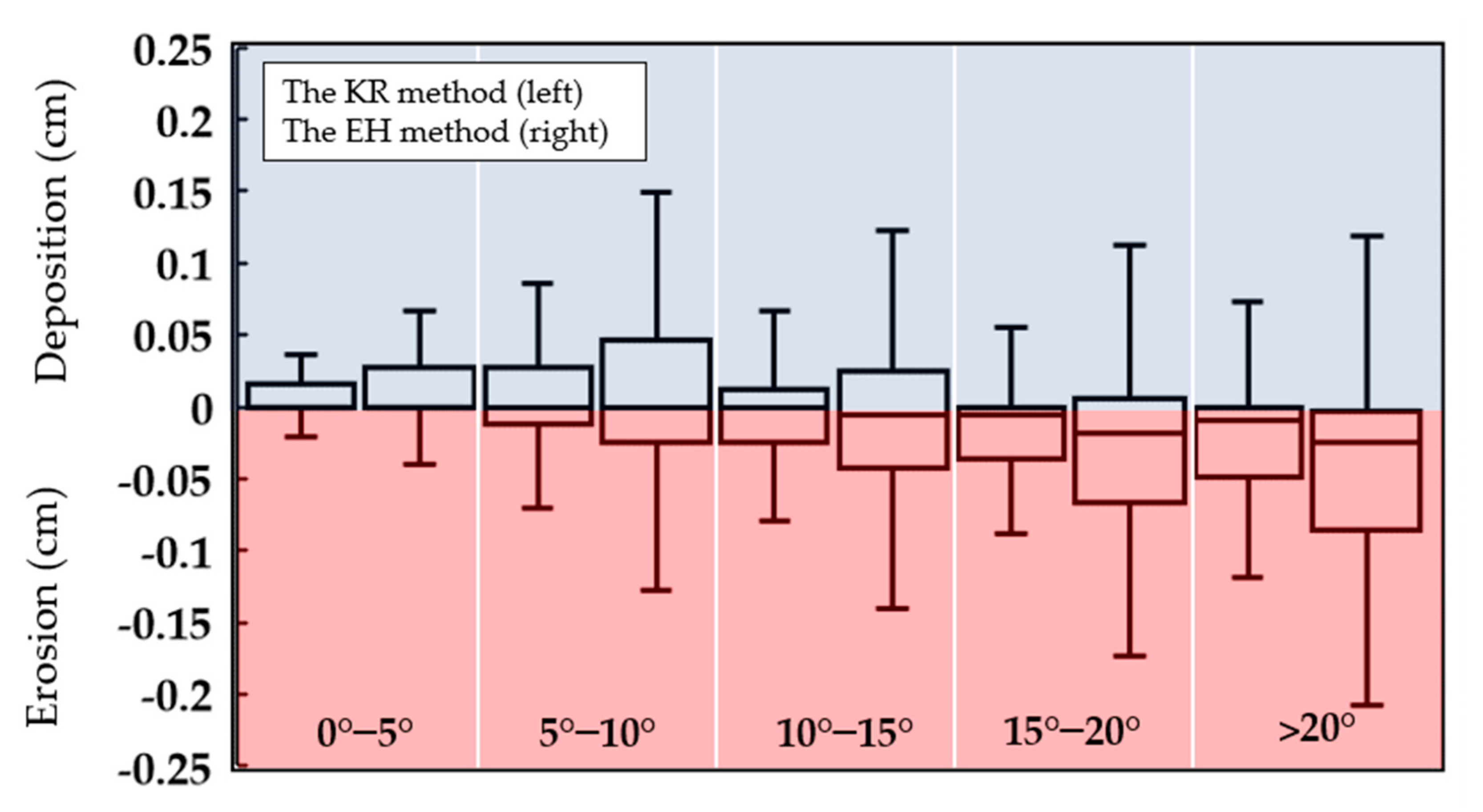
The LULC, soil type, topography, rainfall, and lithology of the bedrock are the main components affecting soil erosion. However, the topography is of significant influence on soil loss [71]. In Figure 8, slope gradients greater than 15° were prone to cause erosion. The augment in slope gradient triggered overland flow velocity and accelerated the transport capacity at these sites [72]. The eroded particles carried by surface runoff were getting weaker and then deposited on evener and flatter sites with slope gradients ranging from 0–5°. The moderate-slope areas (5–15°) considering both erosion and deposition values corresponded to transition sites. These findings are consistent with the previous study of Busacca et al. [73].
Figure 9 reveals the relationship between land-use type and slope gradient. Locations of forest and pasture higher than the remaining land-use type were more strongly related to soil erosion. The box-whisker plots also show that the EH method had a higher influence on topography than the KR method in soil loss spatial distribution, even though both methods had the same results in sediment concentration prediction.
Besides the effect of topography, crop and vegetation stems also affected deposition, notably in agricultural areas. In this watershed, cultivated areas are predominantly located on two sides of rivers. Vegetation stems are instigators that intercept runoff and trap sediment particles [3,27]. Thus, crop stems could contribute a significant influence on the performance of the STC in surface conditions and increase the deposition status of the soil. The spatial distribution patterns of soil organic carbon (SOC) in the watershed (Figure 3d) also indicated that dense SOC content was distinguishable from where the deposition was located. This result is consistent with the study of Zhu et al. [74].
5. Conclusions
In this research, the GSSHA model was deployed to evaluate the rainfall-sediment-runoff process in the Cheoncheon river basin. It is demonstrated that it is possible to reproduce flow discharge over three storm events. Six STC methods were analyzed for simulating sediment concentrations. The principal outcomes are compiled as follows:
(1) From this study, none of the Everaert methods achieved satisfactory results to predict sediment concentrations in three storm events. By allowing the adjustment of an additional parameter, the KR and EH methods surpassed the Everaert methods by producing more accurate results. The KR method also proved to be superior to the EH method when it showed a better performance for sediment concentration simulations with a wide range of sediment size and forcing magnitude.
(2) The spatial distribution of erosion/deposition outputs predicted by the KR and EH methods had similar patterns. While eroded sites were distributed over the watershed, deposited areas were spotted around streams and water bodies. The EH method illustrated the influence of topography on the distribution of erosion/deposition more significantly than the KR method. The results also indicated that the magnitude of soil loss is mild. Slope gradient was the factor spatially contributing to the soil loss distribution. Results depicted that areas with slope gradients ranging from 0°-5° were prone to be deposited. By contrast, erosion was likely to happen with a slope gradient higher than 15°.
The KR method has a simple structure, allowing developers to apply it to their models, whereas the EH method is the only available option for sediment concentration simulations with specific gravity values of particles different from 2.65. However, it is worth noting that applying the EH equation to STC in specific overland-flow areas should be scrutinized conscientiously owing to the divergence in the original establishment of the equation, such as slope gradients and surface conditions. The constraint in the range of sediment sizes and slope gradients contributed to poor performances of the Everaert methods. These formulas could be suited for mild slope areas.
There were some limitations in this study. Firstly, sampling sediment directly in rivers or reservoirs is the most trendy and preferred approach to measure sediment loads with high accuracy. It is not always feasible during extreme storm events due to safety policy and the difficulty of executing such a task. The absence of sediment data has motivated the deployment of sediment rating curves. Nevertheless, such a method is associated with a significant lack of accuracy in extracting sediment loads from flow discharge [75]. Secondly, initial soil moisture values have a significant impact on the results of rainfall-runoff simulation [76]. The wet conditions of soil trigger the overestimation of soil loss, whereas the soil’s dry status leads to the underestimation of sediment concentration for physics-based models [77]. The initial soil moisture data partly affected the results since soil moisture data in this study was provided from the literature. Continuous monitoring of sediment and soil moisture installation is thus essential to reduce data uncertainty and enhance proper evaluation of STC methods since observed datasets of spatial erosion/deposition distribution are excluded in this study.
Soil loss is a worldwide concern contributing to the deterioration of agricultural productivity and water quality. The comprehensive analyses presented above could provide pieces of useful knowledge for choosing an appropriate STC approach to estimate soil erosion/deposition at watershed scales. This can be used as a reference to land-use decision-making and to the design of hydraulic installations for soil conservation.
Author Contributions
Methodology, L.N.V. and G.L.; data curation, M.Y. and S.J.; writing—original draft preparation, L.N.V.; writing—review and editing, L.N.V., X.-H.L. and G.V.N.; supervision, G.L. All authors have read and agreed to the published version of the manuscript.
Funding
This subject is supported by Korea Ministry of Environment as “The SS projects; 2019002830001”.
Institutional Review Board Statement
Not applicable.
Informed Consent Statement
Not applicable.
Data Availability Statement
Data presented in this study are available in Section 2.
Conflicts of Interest
The authors declare no conflict of interest.
Appendix A

Table A1.
Regression equations for flow and sediment discharge: H (water level); Q (river flow); (sediment concentration).
Table A1.
Regression equations for flow and sediment discharge: H (water level); Q (river flow); (sediment concentration).
| Event no. | Rating Curve Equation | Discharge-Sediment Loads Equation |
|---|---|---|
| 1 | Q = 24.945 × (H − 2.281)2.448 | Qs = 9 × 10⁻⁶ − 5 × Q1.700 |
| 2 | Q = 53.522 × (H − 2.346)2.219 | Qs = 5 × 10⁻⁷ − 6 × Q1.932 |
| 3 | Q = 50.403 × (H − 2.367)2.257 | Qs = 28 × 10−7 − 5 × Q1.818 |
Table A2.
Particle size distributions (%) in the Cheoncheon basin.
| Soil Type | Sand | Silt | Clay | |||||
|---|---|---|---|---|---|---|---|---|
| Very Coarse | Coarse | Medium | Fine | Very Fine | Coarse | Fine | ||
| 2.0–1.0 mm | 1.0–0.5 | 0.5–0.25 | 0.25–0.1 | 0.1–0.05 | 0.05–0.02 | 0.02–0.002 | 0.002–0.0002 | |
| Anryong | 2.7 | 5.8 | 5.2 | 5.7 | 3.1 | 36.2 | 13.2 | 28.2 |
| Chilgog | 6.7 | 9 | 7.4 | 6.9 | 3.8 | 23.2 | 19.4 | 23.6 |
| Deogpyeong | 2.6 | 4.8 | 4.1 | 3.4 | 4.3 | 20 | 25 | 35.9 |
| Deogsan | 7.3 | 9.1 | 11.4 | 16.1 | 7.8 | 10.5 | 22.5 | 15.3 |
| Eungog | 15.5 | 21.7 | 15.3 | 12.5 | 5.8 | 9.5 | 10.1 | 9.8 |
| Gacheon | 6.8 | 14.3 | 19.9 | 19.4 | 9.9 | 10 | 12.8 | 7 |
| Gopyeong | 0.5 | 1.1 | 1.1 | 1.5 | 1.1 | 47.4 | 9 | 38.2 |
| Gwanag | 19.6 | 12.5 | 9.4 | 8.3 | 9.5 | 15 | 16.5 | 9.3 |
| Hamo | 3.4 | 4.4 | 5.4 | 8.7 | 4.5 | 20 | 30.7 | 23 |
| Hoegog | 7.5 | 14.2 | 15.1 | 15.3 | 6.8 | 13.1 | 17.4 | 10.6 |
| Hogye | 4.7 | 8.2 | 5.9 | 1.8 | 10.9 | 21 | 18.1 | 29.4 |
| Hwadong | 1.4 | 2.9 | 1.2 | 0.8 | 1.9 | 30 | 27.9 | 34 |
| Hwangryong | 1.4 | 6 | 20.8 | 45.8 | 11.7 | 3.5 | 8.4 | 2.5 |
| Imgog | 2 | 4.3 | 5.9 | 8.9 | 7 | 21.9 | 23.7 | 26.4 |
| Janggye | 3.7 | 7.3 | 10.4 | 16.7 | 11.3 | 13.4 | 20.1 | 17.1 |
| Jigog | 11.2 | 15.6 | 12.9 | 12.2 | 5.2 | 13.5 | 15.2 | 14.3 |
| Maegog | 9.4 | 20.1 | 16.9 | 12.9 | 11.3 | 9.7 | 13.1 | 6.6 |
| Namgye | 17.7 | 19.4 | 15.7 | 15.9 | 5.2 | 9.2 | 7.7 | 9.1 |
| Odae | 25 | 18.3 | 6.9 | 6.3 | 6.1 | 17.2 | 4.6 | 15.4 |
| Oesan | 5.9 | 7.3 | 4.2 | 4 | 2.4 | 28 | 27.4 | 20.8 |
| Osan | 5 | 11 | 0.1 | 9 | 5.2 | 28.9 | 24.6 | 16.2 |
| Pungcheon | 6.5 | 12.6 | 14.3 | 14 | 6.6 | 15.4 | 14.8 | 15.8 |
| Rcs | 6.7 | 9 | 7.4 | 6.9 | 3.8 | 23.2 | 19.4 | 23.6 |
| Rock outcrop | 0.5 | 1.1 | 1.1 | 1.5 | 1.1 | 47.4 | 9 | 38.2 |
| Sachon | 4.9 | 12.9 | 18.5 | 15.4 | 9.1 | 15.3 | 11.4 | 12.4 |
| Samam | 4.2 | 7.4 | 7.8 | 9 | 6.8 | 24.3 | 22.3 | 18.3 |
| Samgag | 16.4 | 17.3 | 13.1 | 6.9 | 6.9 | 11 | 13.9 | 14.6 |
| Sangju | 13.8 | 22.9 | 21.9 | 12.4 | 5.5 | 7.9 | 6.6 | 9 |
| Seogto | 3.8 | 5.3 | 3.7 | 3.4 | 1.9 | 31.6 | 23.4 | 27 |
| Seongin | 4.4 | 9.3 | 11.5 | 6.8 | 3.5 | 25.5 | 17 | 22.1 |
| Songsan | 9.8 | 18.6 | 15.1 | 12.3 | 5 | 10.6 | 11.1 | 17.6 |
| Suam | 7.5 | 10.6 | 16.8 | 22.8 | 14.9 | 10 | 10.6 | 6.9 |
| Ugog | 3.6 | 3.3 | 1.5 | 0.3 | 5.5 | 25 | 30 | 30.9 |
| Water | 2 | 4.3 | 5.9 | 8.9 | 7 | 21.9 | 23.7 | 26.4 |
| Weolgog | 15.5 | 21.7 | 15.3 | 12.5 | 5.8 | 9.5 | 10.1 | 9.8 |
| Yecheon | 15.9 | 16.6 | 10.8 | 10.3 | 5.8 | 14.5 | 11.8 | 14.5 |
| Yesan | 9.7 | 17.4 | 15.3 | 13 | 5.4 | 8.8 | 12.3 | 18 |
| Yonggye | 5.7 | 7.9 | 6.8 | 6.5 | 3.9 | 22 | 21.7 | 25.6 |
References
- Foster, G.G. The Use of Bridging Systems to Increase Genetic Variability in Compound Chromosome Strains for Genetic Control of Lucilia Cuprina (Wiedemann). Theor. Appl. Genet. 1982, 63, 295–305. [Google Scholar] [CrossRef] [PubMed]
- Li, G.; Abrahams, A.D. Controls of Sediment Transport Capacity in Laminar Interrill Flow on Stone-Covered Surfaces. Water Resour. Res. 1999, 35, 305–310. [Google Scholar] [CrossRef]
- Mu, H.; Yu, X.; Fu, S.; Yu, B.; Liu, Y.; Zhang, G. Effect of Stem Basal Cover on the Sediment Transport Capacity of Overland Flows. Geoderma 2019, 337, 384–393. [Google Scholar] [CrossRef]
- Lindström, G.; Pers, C.; Rosberg, J.; Strömqvist, J.; Arheimer, B. Development and Testing of the HYPE (Hydrological Predictions for the Environment) Water Quality Model for Different Spatial Scales. Hydrol. Res. 2010, 41, 295–319. [Google Scholar] [CrossRef]
- Morgan, R.P.C.; Quinton, J.N.; Smith, R.E.; Govers, G.; Poesen, J.W.A.; Auerswald, K.; Chisci, G.; Torri, D.; Styczen, M.E. The European Soil Erosion Model (EUROSEM): A Dynamic Approach for Predicting Sediment Transport from Fields and Small Catchments. Earth Surf. Process. Landf. 1998, 23, 527–544. [Google Scholar] [CrossRef]
- Von Werner, M. Erosion-3D: User Manual, Version. 3.1.1 2006; Geognostics: Berlin, Germany, 2006. [Google Scholar]
- Ewen, J.; Parkin, G.; O’Connell, P.E. SHETRAN: Distributed River Basin Flow and Transport Modeling System. J. Hydrol. Eng. 2000, 5, 250–258. [Google Scholar] [CrossRef] [Green Version]
- USDA-ARS. Revised Universal Soil Loss Equation Version 2 (RUSLE2); (For the Model with Release Date of 20 May 2008); Agricultural Research Service: Washington, DC, USA, 2013. [Google Scholar]
- APIP; Lee, G.; Yu, W.; Jung, K. Catchment-Scale Soil Erosion and Sediment Yield Simulation Using a Spatially Distributed Erosion Model. Env. Earth Sci. 2013, 70, 33–47. [Google Scholar] [CrossRef]
- Wang, S.; Flanagan, D.C.; Engel, B.A. Estimating Sediment Transport Capacity for Overland Flow. J. Hydrol. 2019, 578, 123985. [Google Scholar] [CrossRef]
- Ali, M.; Seeger, M.; Sterk, G.; Moore, D. A Unit Stream Power Based Sediment Transport Function for Overland Flow. Catena 2013, 101, 197–204. [Google Scholar] [CrossRef]
- Ali, M.; Sterk, G.; Seeger, M.; Boersema, M.; Peters, P. Effect of Hydraulic Parameters on Sediment Transport Capacity in Overland Flow over Erodible Beds. Hydrol. Earth Syst. Sci. 2012, 16, 591–601. [Google Scholar] [CrossRef] [Green Version]
- Zhang, G.; Liu, Y.; Han, Y.; Zhang, X.C. Sediment Transport and Soil Detachment on Steep Slopes: I. Transport Capacity Estimation. Soil Sci. Soc. Am. J. 2009, 73, 1291–1297. [Google Scholar] [CrossRef]
- Abrahams, A.D.; Li, G.; Krishnan, C.; Atkinson, J.F. A Sediment Transport Equation for Interrill Overland Flow on Rough Surfaces. Earth Surf. Process. Landf. 2001, 26, 1443–1459. [Google Scholar] [CrossRef]
- Wang, Z.; Yang, X.; Liu, J.; Yuan, Y. Sediment Transport Capacity and Its Response to Hydraulic Parameters in Experimental Rill Flow on Steep Slope. J. Soil Water Conserv. 2015, 70, 36–44. [Google Scholar] [CrossRef] [Green Version]
- Prosser, I.P.; Rustomji, P. Sediment Transport Capacity Relations for Overland Flow. Prog. Phys. Geogr. Earth Environ. 2000, 24, 179–193. [Google Scholar] [CrossRef]
- Everaert, W. Empirical Relations for the Sediment Transport Capacity of Interrill Flow. Earth Surf. Process. Landf. 1991, 16, 513–532. [Google Scholar] [CrossRef]
- Guy, B.T.; Dickenson, W.T.; Sohrabi, T.M.; Rudra, R.P. Development of an Empirical Model for Calculating Sediment-Transport Capacity in Shallow Overland Flows: Model Calibration. Biosyst. Eng. 2009, 103, 245–255. [Google Scholar] [CrossRef]
- Guy, B.T.; Rudra, R.P.; Dickenson, W.T.; Sohrabi, T.M. Empirical Model for Calculating Sediment-Transport Capacity in Shallow Overland Flows: Model Development. Biosyst. Eng. 2009, 103, 105–115. [Google Scholar] [CrossRef]
- Zhang, G.-H.; Wang, L.-L.; Tang, K.-M.; Luo, R.-T.; Zhang, X.C. Effects of Sediment Size on Transport Capacity of Overland Flow on Steep Slopes. Hydrol. Sci. J. 2011, 56, 1289–1299. [Google Scholar] [CrossRef]
- Ni, S.; Feng, S.; Zhang, D.; Wang, J.; Cai, C. Sediment Transport Capacity in Erodible Beds with Reconstituted Soils of Different Textures. Catena 2019, 183, 104197. [Google Scholar] [CrossRef]
- Yu, B.; Zhang, G.; Fu, X. Transport Capacity of Overland Flow with High Sediment Concentration. J. Hydrol. Eng. 2015, 20, C4014001. [Google Scholar] [CrossRef] [Green Version]
- Zhang, G.H.; Wang, L.L.; Li, G.; Tang, K.M.; Cao, Y. Relationship between Sediment Particle Size and Transport Coefficient on Steep Slopes. Trans. ASABE 2011, 54, 869–874. [Google Scholar] [CrossRef]
- Zhan, Z.; Jiang, F.; Chen, P.; Gao, P.; Lin, J.; Ge, H.; Wang, M.K.; Huang, Y. Effect of Gravel Content on the Sediment Transport Capacity of Overland Flow. Catena 2020, 188, 104447. [Google Scholar] [CrossRef]
- Zhang, P.; Yao, W.; Liu, G.; Xiao, P.; Sun, W. Experimental Study of Sediment Transport Processes and Size Selectivity of Eroded Sediment on Steep Pisha Sandstone Slopes. Geomorphology 2020, 363, 107211. [Google Scholar] [CrossRef]
- Gabet, E.J.; Sternberg, P. The Effects of Vegetative Ash on Infiltration Capacity, Sediment Transport, and the Generation of Progressively Bulked Debris Flows. Geomorphology 2008, 101, 666–673. [Google Scholar] [CrossRef]
- Pan, C.; Ma, L.; Shangguan, Z. Effectiveness of Grass Strips in Trapping Suspended Sediments from Runoff. Earth Surf. Process. Landf. 2010, 35, 1006–1013. [Google Scholar] [CrossRef]
- Englelund, F.; Hansen, E. A Monograph on Sediment Transport in Alluvial Streams; Teknisk Forlag: Copenhagen, Denmark, 1967; p. 65. [Google Scholar]
- Yalin, M.S. An Expression for Bed-Load Transportation. J. Hydraul. Div. 1963, 89, 221–250. [Google Scholar] [CrossRef]
- Smart, G.M. Sediment Transport Formula for Steep Channels. J. Hydraul. Eng. 1984, 110, 267–276. [Google Scholar] [CrossRef]
- Seng Low, H. Effect of Sediment Density on Bed-Load Transport. J. Hydraul. Eng. 1989, 115, 124–138. [Google Scholar] [CrossRef]
- Hessel, R.; Jetten, V. Suitability of Transport Equations in Modelling Soil Erosion for a Small Loess Plateau Catchment. Eng. Geol. 2007, 91, 56–71. [Google Scholar] [CrossRef]
- Kilinc, M.; Richardson, E.V. Mechanics of Soil Erosion From Overland Flow Generated; Colorado State University: Fort Colins, CO, USA, 1973; p. 61. [Google Scholar]
- Guy, B.T.; Dickinson, W.T.; Rudra, R.P. Evaluation of Fluvial Sediment Transport Equations for Overland Flow. Trans. ASAE 1992, 35, 545–555. [Google Scholar] [CrossRef]
- Yang, C.T. Unit Stream Power and Sediment Transport. J. Hydraul. Div. 1972, 98, 1805–1826. [Google Scholar] [CrossRef]
- Govers, G. Empirical Relationships on the Transporting Capacity of Overland Flow. In Transport and Deposition Processes (Proceedings of the Jerusalem Workshop, March–April 1987); IAHS Press: Wallingford, UK, 1990; Volume 189, pp. 45–63. [Google Scholar]
- Downer, C.W.; Pradhan, N.R.; Ogden, F.L.; Byrd, A.R. Testing the Effects of Detachment Limits and Transport Capacity Formulation on Sediment Runoff Predictions Using the U.S. Army Corps of Engineers GSSHA Model. J. Hydrol. Eng. 2015, 20, 04014082. [Google Scholar] [CrossRef]
- Sith, R.; Nadaoka, K. Comparison of SWAT and GSSHA for High Time Resolution Prediction of Stream Flow and Sediment Concentration in a Small Agricultural Watershed. Hydrology 2017, 4, 27. [Google Scholar] [CrossRef] [Green Version]
- Ogden, F.L. Evidence of Equilibrium Peak Runoff Rates in Steep Tropical Terrain on the Island of Dominica during Tropical Storm Erika, 27 August 2015. J. Hydrol. 2016, 542, 35–46. [Google Scholar] [CrossRef] [Green Version]
- Pradhan, N.R.; Loney, D. An Analysis of the Unit Hydrograph Peaking Factor: A Case Study in Goose Creek Watershed, Virginia. J. Hydrol. Reg. Stud. 2018, 15, 31–48. [Google Scholar] [CrossRef]
- Saha, G.C.; Li, J.; Thring, R.W.; Hirshfield, F.; Paul, S.S. Temporal Dynamics of Groundwater-Surface Water Interaction under the Effects of Climate Change: A Case Study in the Kiskatinaw River Watershed, Canada. J. Hydrol. 2017, 551, 440–452. [Google Scholar] [CrossRef]
- Hur, J.; Jung, N.-C.; Shin, J.-K. Spectroscopic Distribution of Dissolved Organic Matter in a Dam Reservoir Impacted by Turbid Storm Runoff. Environ. Monit Assess 2007, 133, 53–67. [Google Scholar] [CrossRef]
- Hong, S.Y.; Zhang, Y.-S.; Hyun, B.-K.; Sonn, Y.-K.; Kim, Y.-H.; Jung, S.-J.; Park, C.-W.; Song, K.-C.; Jang, B.-C.; Choe, E.-Y.; et al. An Introduction of Korean Soil Information System. Korean J. Soil Sci. Fertil. 2009, 42, 21–28. [Google Scholar]
- USDA. Soil Taxonomy: A Basic System of Soil Classification for Making and Interpreting Soil Surveys; USDA: Washington, DC, USA, 1999. [Google Scholar]
- Sastre, B.; Barbero-Sierra, C.; Bienes, R.; Marques, M.J.; García-Díaz, A. Soil Loss in an Olive Grove in Central Spain under Cover Crops and Tillage Treatments, and Farmer Perceptions. J Soils Sediments 2017, 17, 873–888. [Google Scholar] [CrossRef]
- K-Water. Hydrological Investigation Report of Yongdam Dam Basin; Korean Water and Wastewater Association: Seoul, Korea, 2002. [Google Scholar]
- K-Water. Hydrological Investigation Report of Yongdam Dam Basin; Korean Water and Wastewater Association: Seoul, Korea, 2003. [Google Scholar]
- K-Water. Hydrological Investigation Report of Yongdam Dam Basin; Korean Water and Wastewater Association: Seoul, Korea, 2007. [Google Scholar]
- Julien, P.Y. Erosion and Sedimentation; Cambridge University Press: Cambridge, UK, 1995. [Google Scholar]
- Ogden, F.; Heilig, A. Two-Dimensional Watershed-Scale Erosion Modeling With CASC2D. In Landscape Erosion and Evolution Modeling; Harmon, R.S., Doe, W.W., Eds.; Springer US: Boston, MA, USA, 2001; pp. 277–320. ISBN 978-1-4613-5139-9. [Google Scholar]
- Downer, C.W.; Ogden, F.L. GSSHA: Model To Simulate Diverse Stream Flow Producing Processes. J. Hydrol. Eng. 2004, 9, 161–174. [Google Scholar] [CrossRef]
- The Complete All-in-one Watershed Solution. Available online: https://www.aquaveo.com/software/wms-watershed-modeling-system-introduction (accessed on 8 July 2021).
- Wicks, J.M.; Bathurst, J.C. SHESED: A Physically Based, Distributed Erosion and Sediment Yield Component for the SHE Hydrological Modelling System. J. Hydrol. 1996, 175, 213–238. [Google Scholar] [CrossRef]
- Capra, A.; Porto, P.; Scicolone, B. Relationships between Rainfall Characteristics and Ephemeral Gully Erosion in a Cultivated Catchment in Sicily (Italy). Soil Tillage Res. 2009, 105, 77–87. [Google Scholar] [CrossRef]
- ESRI. ESRI Data and Maps for ArcGIS; Environmental Systems Research Institute: Redlands, CA, USA, 2021. [Google Scholar]
- Lee, G.; Tachikawa, Y.; Takara, K. Interaction between Topographic and Process Parameters Due to the Spatial Resolution of DEMs in Distributed Rainfall-Runoff Modeling. J. Hydrol. Eng. 2009, 14, 1059–1069. [Google Scholar] [CrossRef]
- Duan, Q.Y.; Gupta, V.K.; Sorooshian, S. Shuffled Complex Evolution Approach for Effective and Efficient Global Minimization. J. Optim. Theory Appl. 1993, 76, 501–521. [Google Scholar] [CrossRef]
- Downer, C.W.; Ogden, F.L. Gridded Surface Subsurface Hydrologic Analysis (GSSHA) User’s Manual; U.S. Army Corps of Engineers: Washington, DC, USA, 2006. [Google Scholar]
- Gupta, H.V.; Sorooshian, S.; Yapo, P.O. Status of Automatic Calibration for Hydrologic Models: Comparison with Multilevel Expert Calibration. J. Hydrol. Eng. 1999, 4, 135–143. [Google Scholar] [CrossRef]
- Du, J.; Xie, S.; Xu, Y.; Xu, C.; Singh, V.P. Development and Testing of a Simple Physically-Based Distributed Rainfall-Runoff Model for Storm Runoff Simulation in Humid Forested Basins. J. Hydrol. 2007, 336, 334–346. [Google Scholar] [CrossRef]
- Johnson, B.E.; Julien, P.Y.; Molnar, D.K.; Watson, C.C. The two-dimensional upland erosion model CASC2D-SED. J. Am. Water Resour. Assoc. 2000, 36, 31–42. [Google Scholar] [CrossRef]
- Lei, T.W.; Zhang, Q.; Zhao, J.; Tang, Z. A Laboratory Study of Sediment Transport Capacity in the Dynamic Process of Rill Erosion. Trans. Am. Soc. Agric. Eng. 2001, 44, 1537–1542. [Google Scholar]
- Xiao, H.; Liu, G.; Liu, P.; Zheng, F.; Zhang, J.; Hu, F. Sediment Transport Capacity of Concentrated Flows on Steep Loessial Slope with Erodible Beds. Sci. Rep. 2017, 7, 1–9. [Google Scholar] [CrossRef] [PubMed]
- Zhang, F.B.; Yang, M.Y.; Li, B.B.; Li, Z.B.; Shi, W.Y. Effects of Slope Gradient on Hydro-Erosional Processes on an Aeolian Sand-Covered Loess Slope under Simulated Rainfall. J. Hydrol. 2017, 553, 447–456. [Google Scholar] [CrossRef]
- Lu, J.Y.; Cassol, E.A.; Moldenhauer, W.C. Sediment Transport Relationships for Sand and Silt Loam Soils. Trans. ASAE 1989, 32, 1923. [Google Scholar] [CrossRef]
- Alonso, C.V.; Neibling, W.H.; Foster, G.R. Estimating Sediment Transport Capacity in Watershed Modeling. Trans. ASAE 1981, 24, 1211–1220. [Google Scholar] [CrossRef]
- Chen, C.-N.; Tfwala, S.S.; Tsai, C.-H. Climate Change Impacts on Soil Erosion and Sediment Yield in a Watershed. Water 2020, 12, 2247. [Google Scholar] [CrossRef]
- Routschek, A.; Schmidt, J.; Kreienkamp, F. Impact of Climate Change on Soil Erosion—A High-Resolution Projection on Catchment Scale until 2100 in Saxony/Germany. Catena 2014, 121, 99–109. [Google Scholar] [CrossRef]
- Yu, W.; Lee, G.; Kim, Y.; Jung, K. Watershed-Based PMF and Sediment-Runoff Estimation Using Distributed Hydrological Model. J. Korean Soc. Agric. Eng. 2018, 60, 1–11. [Google Scholar]
- Li, G.; Wan, L.; Cui, M.; Wu, B.; Zhou, J. Influence of Canopy Interception and Rainfall Kinetic Energy on Soil Erosion under Forests. Forests 2019, 10, 509. [Google Scholar] [CrossRef] [Green Version]
- Wu, L.; Peng, M.; Qiao, S.; Ma, X. Effects of Rainfall Intensity and Slope Gradient on Runoff and Sediment Yield Characteristics of Bare Loess Soil. Environ. Sci. Pollut. Res. 2018, 25, 3480–3487. [Google Scholar] [CrossRef] [PubMed]
- Fox, D.M.; Bryan, R.B. The Relationship of Soil Loss by Interrill Erosion to Slope Gradient. Catena 2000, 38, 211–222. [Google Scholar] [CrossRef]
- Busacca, A.J.; Cook, C.A.; Mulla, D.J. Comparing Landscape-Scale Estimation of Soil Erosion in the Palouse Using Cs-137 and RUSLE. J. Soil Water Conserv. 1993, 48, 361–367. [Google Scholar]
- Zhu, Y.; Wang, D.; Wang, X.; Li, W.; Shi, P. Aggregate-Associated Soil Organic Carbon Dynamics as Affected by Erosion and Deposition along Contrasting Hillslopes in the Chinese Corn Belt. Catena 2021, 199, 105106. [Google Scholar] [CrossRef]
- Walling, D.E.; Webb, B.W. The Reliability of Rating Curve Estimates of Suspended Sediment Yield: Some Further Comments. In Proceedings of the Symposium on Sediment Budgets, Porto Alegre, Brazil, 11–15 December 1988. [Google Scholar]
- Zehe, E.; Becker, R.; Bárdossy, A.; Plate, E. Uncertainty of Simulated Catchment Runoff Response in the Presence of Threshold Processes: Role of Initial Soil Moisture and Precipitation. J. Hydrol. 2005, 1–4, 183–202. [Google Scholar] [CrossRef]
- Ahmadi, S.H.; Amin, S.; Reza Keshavarzi, A.; Mirzamostafa, N. Simulating Watershed Outlet Sediment Concentration Using the ANSWERS Model by Applying Two Sediment Transport Capacity Equations. Biosyst. Eng. 2006, 94, 615–626. [Google Scholar] [CrossRef]
Figure 1.
The schematic diagram of the study.

Figure 2.
Location of the Cheoncheon watershed.

Figure 3.
(a) Land use type; (b) Soil type; (c) DEM; (d) Soil organic carbon; (e) Slope gradient.

Figure 4.
Flow discharge predicted by the GSSHA model in Event 1 (a), Event 2 (b), and Event 3 (c). The scatter plots (and values) represent a 1:1 comparison between the prediction (y-axis) and the observation (x-axis), and the black lines denote the stream discharge.
Figure 4.
Flow discharge predicted by the GSSHA model in Event 1 (a), Event 2 (b), and Event 3 (c). The scatter plots (and values) represent a 1:1 comparison between the prediction (y-axis) and the observation (x-axis), and the black lines denote the stream discharge.

Figure 5.
Comparison between simulation and observation of sediment concentrations in Cheoncheon basin with the KR method in Event 1 (a), Event 2 (b), and Event 3 (c); with the EH method in Event 1 (d), Event 2 (e), and Event 3 (f).
Figure 5.
Comparison between simulation and observation of sediment concentrations in Cheoncheon basin with the KR method in Event 1 (a), Event 2 (b), and Event 3 (c); with the EH method in Event 1 (d), Event 2 (e), and Event 3 (f).

Figure 6.
Spatial-temporal distribution of erosion/deposition maps predicted by the KR method in Event 1 (a), Event 2 (b), and Event 3 (c); and by the EH method in Event 1 (d), Event 2 (e), and Event 3 (f).
Figure 6.
Spatial-temporal distribution of erosion/deposition maps predicted by the KR method in Event 1 (a), Event 2 (b), and Event 3 (c); and by the EH method in Event 1 (d), Event 2 (e), and Event 3 (f).

Figure 7.
Area of erosion/deposition (in %) corresponding to various magnitudes predicted by the KR method (in red) and the EH method (in blue).
Figure 7.
Area of erosion/deposition (in %) corresponding to various magnitudes predicted by the KR method (in red) and the EH method (in blue).

Figure 8.
Boxplots of slope gradients show erosion/deposition behavior in three events. In each boxplot, the central line is the median, whereas the edges of the boxes denote the 25th and 75th percentiles, respectively. The upper and lower whiskers denote the maximum and minimum, respectively.
Figure 8.
Boxplots of slope gradients show erosion/deposition behavior in three events. In each boxplot, the central line is the median, whereas the edges of the boxes denote the 25th and 75th percentiles, respectively. The upper and lower whiskers denote the maximum and minimum, respectively.

Figure 9.
The interrelation between slope gradient (a) and land-use type (b) toward soil ero-sion/deposition in three events is demonstrated by boxplots.
Figure 9.
The interrelation between slope gradient (a) and land-use type (b) toward soil ero-sion/deposition in three events is demonstrated by boxplots.

Table 1.
Particle-size properties for the study.
| Description | Particle Diameter (mm) | Particle Size Distribution (%) |
|---|---|---|
| Very coarse sand | 1.45 | Table A2 |
| Coarse sand | 0.65 | |
| Medium sand | 0.37 | |
| Fine sand | 0.17 | |
| Very fine sand | 0.08 | |
| Coarse silt | 0.03 | |
| Fine silt | 0.011 | |
| Clay | 0.003 |
Table 2.
Description of three storm events.
| Event Number | Total Duration (Hour) | Total Rainfall (mm) | Peak Rainfall (mm) | Number of Peaks | Name of Events | Description |
|---|---|---|---|---|---|---|
| 1 | 75 | 194.8 | 27 | 1 | Rusa | Calibration |
| 2 | 92 | 133.9 | 26 | 2 | Maemi | Validation |
| 3 | 178 | 205.5 | 48 | 2 | Nari | Validation |
Table 3.
Information about the data used in this study.
| Data Layer | Description | Data Source |
|---|---|---|
| Meteorological data | Hourly precipitation | Water Resources Management Information System (http://wamis.go.kr/) |
| Soil type data | 30 × 30m resolution | Korean Soil Information System (http://soil.rda.go.kr/) |
| Land use/land cover data | NASA’s EarthExplorer web service (http://earthexplorer.usgs.gov/) | |
| DEM data |
Table 4.
Calibrated parameters used in the GSSHA model for flow discharge prediction.
| Parameter | Land Use/Soil Type | Range of Values | Optimal Value |
|---|---|---|---|
| Surface roughness (manning’s n) | Mixed forest | 0.05–0.6 | 0.1921 |
| Mixed field | 0.03–0.2 | 0.1676 | |
| Retention depth (mm) | Mixed forest | 0.1–10.0 | 5.0739 |
| Mixed field | 0.1–10.0 | 6.6658 | |
| Hydraulic conductivity (cm/h) | Oesan | 0.01–3.0 | 0.0573 |
| Samgag | 0.01–1.0 | 0.0871 | |
| Soil moisture depth (m) | 0.1–1.0 | 0.8948 | |
| Top layer depth (m) | 0.03–0.3 | 0.1197 | |
| Channel roughness (manning’s n) | 0.0245–0.0365 | 0.0274 |
Table 5.
Statistical analysis of observed and simulated values of flow discharge.
| Event | RMSE (m3/s) | PBIAS (%) | VCI | |
|---|---|---|---|---|
| 1 | 0.90 | 116.79 | 20.17 | 0.998 |
| 2 | 0.92 | 76.32 | 60.02 | 0.505 |
| 3 | 0.73 | 96.67 | 61.47 | 0.385 |
Table 6.
Statistical analysis of observed and predicted values of sediment concentrations.
| Method | Event | RMSE (mg/L) | PBIAS (%) | VCI | |
|---|---|---|---|---|---|
| 1 | 0.83 | 532.65 | 20.17 | 0.798 | |
| KR | 2 | 0.80 | 778.63 | 60.12 | 0.401 |
| 3 | 0.58 | 918.96 | 66.49 | 0.335 | |
| 1 | 0.77 | 599.65 | 11.55 | 0.885 | |
| EH | 2 | 0.75 | 816.76 | 58.79 | 0.412 |
| 3 | 0.46 | 946.31 | 69.06 | 0.309 | |
| 1 | - | 1193.21 | 96.01 | 0.262 | |
| USP | 2 | - | 1368.87 | 96.66 | 0.033 |
| 3 | - | 2471.68 | 73.85 | 0.039 | |
| 1 | - | 1293.95 | −0.15 | 1.001 | |
| ESP | 2 | - | 1080.04 | 69.27 | 0.307 |
| 3 | - | 4771.54 | −2.93 | 1.029 | |
| 1 | - | 203,673 | −13,235.5 | 133.35 | |
| SUD | 2 | - | 98,484 | −5826.61 | 59.2 |
| 3 | - | 112,527 | −4852.65 | 49.5 | |
| 1 | - | 12,854,268 | −1,249,831 | 14,342 | |
| SV | 2 | - | 28,149,108 | −1,740,866 | 26,384 |
| 3 | 1 | 38,661,463 | −736,509 | 34,976 |
1 minimal value of R2.
Publisher’s Note: MDPI stays neutral with regard to jurisdictional claims in published maps and institutional affiliations. |
© 2021 by the authors. Licensee MDPI, Basel, Switzerland. This article is an open access article distributed under the terms and conditions of the Creative Commons Attribution (CC BY) license (https://creativecommons.org/licenses/by/4.0/).
Share and Cite
MDPI and ACS Style
Van, L.N.; Le, X.-H.; Nguyen, G.V.; Yeon, M.; Jung, S.; Lee, G. Investigating Behavior of Six Methods for Sediment Transport Capacity Estimation of Spatial-Temporal Soil Erosion. Water 2021, 13, 3054. https://doi.org/10.3390/w13213054
AMA Style
Van LN, Le X-H, Nguyen GV, Yeon M, Jung S, Lee G. Investigating Behavior of Six Methods for Sediment Transport Capacity Estimation of Spatial-Temporal Soil Erosion. Water. 2021; 13(21):3054. https://doi.org/10.3390/w13213054
Chicago/Turabian StyleVan, Linh Nguyen, Xuan-Hien Le, Giang V. Nguyen, Minho Yeon, Sungho Jung, and Giha Lee. 2021. "Investigating Behavior of Six Methods for Sediment Transport Capacity Estimation of Spatial-Temporal Soil Erosion" Water 13, no. 21: 3054. https://doi.org/10.3390/w13213054
Note that from the first issue of 2016, this journal uses article numbers instead of page numbers. See further details here.