
Raspy-Cal: A Genetic Algorithm-Based Automatic Calibration Tool for HEC-RAS Hydraulic Models


1
Department of Civil and Environmental Engineering, Colorado School of Mines, Golden, CO 80401, USA
2
Shiley School of Engineering, University of Portland, Portland, OR 97203, USA
3
Research Applications Laboratory, National Center for Atmospheric Research, Boulder, CO 80305, USA
*
Author to whom correspondence should be addressed.
Water 2021, 13(21), 3061; https://doi.org/10.3390/w13213061
Submission received: 27 September 2021
/
Revised: 29 October 2021
/
Accepted: 31 October 2021
/
Published: 2 November 2021
(This article belongs to the Section Hydraulics and Hydrodynamics)
Abstract
:While automatic calibration programs exist for many hydraulic models, no user-friendly and broadly reusable automatic calibration system currently exists for steady-state HEC-RAS models. This study highlights development of Raspy-Cal, an automatic HEC-RAS calibration program based on a genetic algorithm and implemented in Python. It includes a graphical user interface and an interactive command-line interface, as well as libraries readily usable by other programs. As a case study, Raspy-Cal was used to calibrate a model of the Los Angeles River in California and its two major tributaries. We found that Raspy-Cal matched the accuracy of manual calibrations in much less time and without manual intervention, producing a Nash–Sutcliffe Efficiency of 0.89 or greater within several hours when run for 100 iterations. Our analysis showed that the open-source freeware facilitates fast and precise calibration of HEC-RAS models and could serve as a basis for future software development. Raspy-Cal is available online in source and executable form as well as through the Python Package Index.
1. Introduction
Hydraulic modeling is used to observe and predict the behavior of surface waters under specified flow conditions. Hydraulic models can in turn be used to plan for flood management scenarios or to support environmental analyses, such as evaluating the effects of flow scenarios on habitat suitability and ecological responses [1,2,3]. One commonly-used model is the Hydraulic Engineering Center’s River Analysis System (HEC-RAS), which is developed and supported by the U.S. Army Corps of Engineers [4]. HEC-RAS steady-state simulations use Manning’s equation, expansion and contraction coefficients, and the momentum equation to simulate a variety of hydraulic variables such as depth, velocity, and shear stress [5]. It is best practice to calibrate hydraulic models to observed data, such as stage and discharge, to produce accurate results. In the case of a one-dimensional HEC-RAS model, a typical calibration parameter is Manning’s roughness coefficient, n (e.g., [6,7,8]), which, as a coefficient in the calculation of the flow rate, has a significant effect on predicted hydraulic behavior. In cases of large spatial domains, manual calibration of HEC-RAS models can be computationally expensive and time-consuming. This work introduces an efficient, user-friendly, and open-source automatic calibration tool capable of fully calibrating the roughness coefficient without user intervention.
Optimization algorithms for automatic calibration of the roughness coefficient in hydraulic models have been widely studied [9,10,11,12]. Heuristic algorithms, such as genetic algorithms, are commonly used for calibration of hydrologic models (e.g., [9,10,11,13]), and have also been demonstrated to be effective for hydraulic models. For example, Lin et al. [12] used the heuristic algorithm Dynamically-Dimensioned Search (DDS) to calibrate an unsteady flow hydraulic model, Complex-Compound Channel Flow Modeling by the Multimode Method of Characteristics (CCCMMOC), for Manning’s roughness coefficient. They concluded that the approach taken was both effective and efficient for determining optimal roughness coefficients. However, this approach is not easily reproducible or integrated into HEC-RAS.
HEC-RAS can be controlled by other Windows programs using its Component Object Module (COM) interface, called HECRASController [4]; the direct use of the controller, such as through Excel or MATLAB, is well-documented [14,15], but it does not provide an integrated calibration utility. A proof-of-concept of automatic HEC-RAS calibration with a Python script connecting to HECRASController was provided by Dysarz [16]. The code presented therein [16] is provided in the form of a collection of short, one-off scripts, which provide a useful example of how to implement HEC-RAS automatic calibration, but are not reusable for general calibration purposes and do not provide a user interface.
Dysarz [16] and numerous studies involving the calibration of HEC-RAS models (e.g., [7,8,15,17]) provide examples for, and demonstrate interest in, a reusable HEC-RAS automatic calibration framework. In addition, development of a HEC-RAS automation library in Python, PyRas, was started by Peña-Castellanos [18]. However, the code developed by Dysarz [16] is, in accordance with the paper’s stated purpose of demonstrating techniques, not particularly reusable or generic, while PyRas [18] seems to be incomplete and has apparently not been maintained since 2015, making it a risky foundation for new development.
HEC-RAS itself provides an automatic calibration system [19], but the built-in tool only works in unsteady state, which tends to be unstable for large model domains. An automatic calibration system that runs in steady state permits the efficient calibration of much larger models than are feasible with unsteady state simulation. In addition, the built-in automatic calibrator only supports calibration by average error and Root Mean Square Error (RMSE), with no options for trend-based metrics, multi-objective optimization, or interactive calibration.
The purpose of this paper is to present the development procedure of, and a case study with, a free and open-source HEC-RAS automatic calibration tool (Raspy-Cal) along with its default automation module (Raspy), which is also available as a standalone library. Each of these independently has further utility, for calibration of other models and for additional HEC-RAS automation tasks, respectively. Raspy-Cal supports both interactive and fully automatic calibration using a variety of goodness of fit metrics. In the interactive mode, the user runs a set of solutions and is presented with a selection of the best ones, which they evaluate to specify a new range of solutions until the result is satisfactory. In automatic mode, the tool adopts the approach used by others ([9,10]) of using the Nondominated Sorting Genetic Algorithm II (NSGA-II [20]) to find solutions that are non-dominated in terms of selected goodness of fit metrics. The tool provides a range of goodness of fit metrics and is designed to allow easy addition of others.
Both Raspy-Cal and its default automation module Raspy are available for use under an open-source license, which encourages development contributions from other researchers and engineers and allows the tools to continue improving with new developments in calibration techniques and future versions of HEC-RAS. The GNU General Public License v3.0 used for both Raspy-Cal and Raspy allows use, modification, and redistribution as long as any derivatives are released under the same license. Raspy-Cal is available for download at raspy-cal.dphilippus.com (accessed on 26 September 2021), which also provides a link to Raspy as a standalone module, and can be installed from the Python Package Index as raspy-cal.
As a case study, we used our tool to calibrate a one-dimensional hydraulic model of the Los Angeles River and two tributaries that were previously manually calibrated. A variety of individual fit metrics and combinations thereof were compared with automatic calibration. We found Raspy-Cal, run with Nash–Sutcliffe Efficiency and Root Mean Square Error as the error metrics, to be faster and at least as accurate as manual calibration.
2. Materials and Methods
2.1. General Automation (Raspy)
To support automatic calibration, it is necessary to be able to run the model, retrieve results, and modify parameters automatically; for example, a similar, though more extensive, automation system for the watershed model Hydrological Simulation Program in FORTRAN (HSPF), also implemented in Python, is described in Lampert and Wu [21]. The Raspy-Cal software was developed modularly such that the relevant capabilities were developed separately from the calibration algorithm. This has the advantage of allowing independent use of the automation framework for tasks other than calibration. We built the automation functionality around the HEC-RAS COM interface, HECRASController, which allows other Windows programs to use HEC-RAS functions such as retrieving flow data for a node, setting the roughness coefficient, or running simulations. To readily use the COM interface from Python, we developed a Python wrapper around the interface as the lowest-level module of Raspy. The wrapper provides documentation and clarifies arguments and return values.
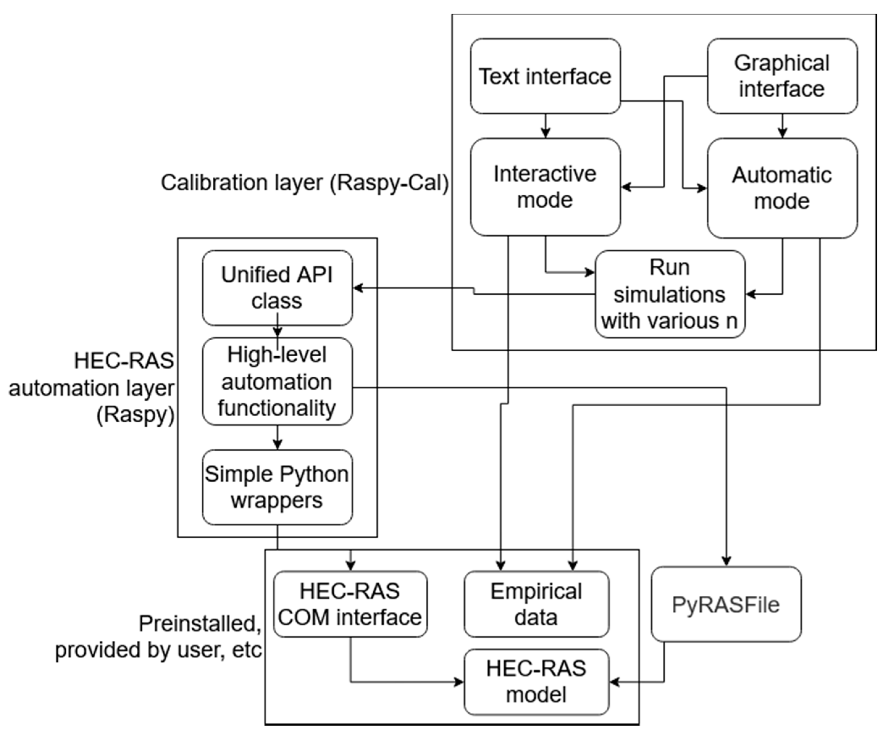
The Python wrapper is the foundation for a more abstract layer, which interfaces with HEC-RAS but hides the internal details to provide model-agnostic functionality. This interface in turn can be easily used by programs such as the calibration tool, with the abstraction meaning that front-end users do not need to know the implementation details. In the wrapper module, we use PyRASFile (https://github.com/larflows/pyrasfile, accessed on 26 September 2021) HEC-RAS file writing and parsing functions for setting the range of discharges to be modeled (flow profiles) where the COM interface proved to be prone to crashing. The use of these dependencies is shown in Figure 1.
Using the COM wrapper and PyRASFile functions, the main portion of Raspy implements a unified Application Program Interface (API) object that provides a variety of methods grouped as parameter modifiers, data retrievers, and operations tools. Parameter modifiers are used to set roughness coefficients and flow profiles, data retrievers to retrieve flow data, and operations tools to run simulations. The methods provided by this API class are designed to allow the calibration module to be written in a model-agnostic way. Because of this, users input information that is, as much as possible, applicable to any model and not specific to the hydraulic model used. The architecture of Raspy-Cal, including Raspy, is shown in Figure 1.
2.2. Calibration (Raspy-Cal)
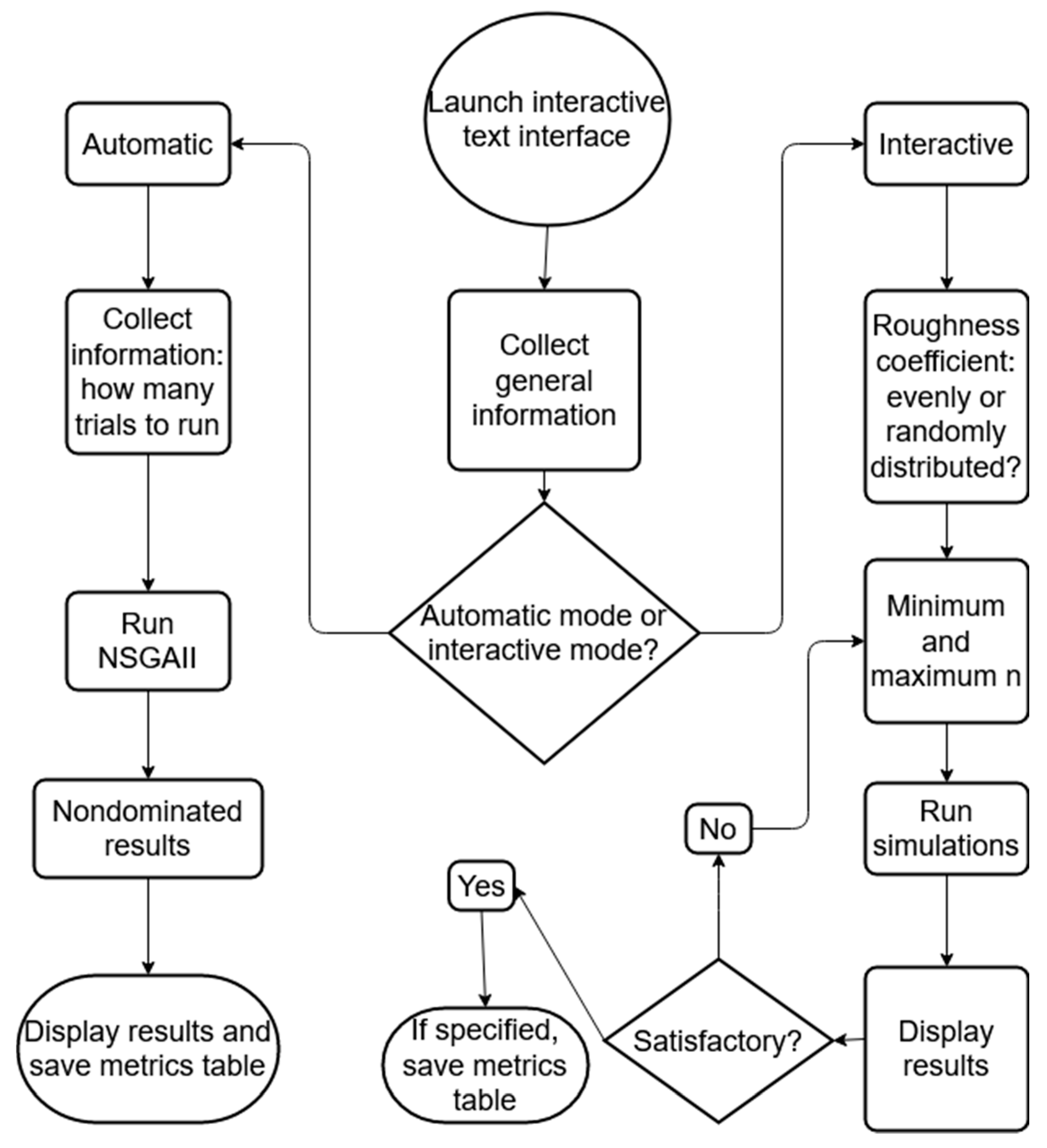
The Raspy automation module provides a reference and default implementation of the automation functionality required by the calibration module of Raspy-Cal. Raspy-Cal’s calibration module centers on running a user-specified number of simulations with a variety of roughness coefficients and retrieving the results for comparison to empirical data. The process of using Raspy-Cal is illustrated in Figure 2. The simulations and data retrieval are done using a provided model object, which by default is the Raspy module’s API object. The sole dependency of Raspy-Cal on Raspy is a “default model” function that can easily be switched out. This modular design allows easy use of different models or automation implementations.
The core suite of functions performs three basic tasks. The first function, the central component for running multiple simulations, runs the model with a given set of roughness coefficients and returns the stage height for each flow value for each coefficient. The second set of functions generates roughness coefficients to test according to user specifications, and the third set of functions produces a set of goodness of fit metrics between empirical and simulated data.
The core functions are used to support the two calibration modes, interactive and automatic. In both cases, the user provides a prepared model with geometry data. The user can then either provide a file containing empirical rating curve data or, if applicable, the United States Geological Survey (USGS) gage number for the calibration cross-section. If a USGS gage number is specified, the tool will automatically retrieve a range of rating curve points from the last two years’ worth of USGS data by default [22], selected such that the flow values are roughly evenly distributed across the full range on a log scale. Specification of the exact date range to use and how many values to use is possible through the command-line version of the tool.
In interactive (manual) mode, the user specifies a range of roughness coefficients, how many to test, and whether to use evenly distributed or randomly generated coefficients within the range. The user also specifies which metrics to use out of the root mean squared error (RMSE), the coefficient of determination, percent bias, the Kolmogorov–Smirnov statistic, the paired t-test, mean absolute error (MAE), and Nash–Sutcliffe Efficiency (NSE) [23,24,25]. The tool runs the model with all the roughness coefficients, then chooses all the non-dominated results based on the chosen metrics. The metrics are provided by the HydroErr and SciPy libraries [26,27], with the exception of percent bias, which is implemented in the code based on the equivalent R language function provided by R language’s hydroGOF hydrology goodness of fit library [28]. Matplotlib [29] is used to generate plots from the simulation. The tool displays a table of the non-dominated roughness coefficients and their fit metrics as well as a plot comparing the rating curves for the best-fitting coefficients to the empirical rating curve. Based on error metric results (table) and the accompanying visualization (plot), the user specifies a new range of roughness coefficients, and iterates until a satisfactory result is found.
In automatic mode, the user similarly specifies which error metrics to use as optimization objectives, as well as the number of simulations to run and the number of roughness coefficients to evaluate each time. The tool then uses the NSGA-II multi-objective genetic algorithm [20] to find optimal results within the number of trials specified, in order to converge on a Pareto-optimal set of coefficients. We chose the NSGA-II algorithm because it is an efficient algorithm for identifying optimal solutions according to multiple objectives and it has been used for similar water resources applications [9,10], while genetic algorithms in general have also found applications in other civil engineering optimization problems [30]. Compared to classical multi-objective optimization algorithms, NSGA-II fares better when the problem space tends towards local optima [31]. Reducing the tendency towards local optima makes initial conditions less important and makes the Raspy-Cal calibration module more generalizable to applications where distinct local optima are likely. The platypus-opt package [32] is used as the implementation of NSGA-II. After all the trials are run, the program displays a fit metric table and rating curve comparison plot as in interactive mode. The processes for both modes are shown in Figure 2.
Raspy-Cal as currently developed does not support automatic validation. However, the user can validate the calibrated results by setting the empirical data as the validation data and running a single iteration in interactive mode with the roughness coefficient range set to the calibrated value. Raspy-Cal also exports the raw data for the optimal results in CSV format, which can be used for manual validation outside of the tool.
Early testing of Raspy-Cal showed that differences in datum with regards to stage could cause significant issues in calibration. Therefore, an option for datum adjustment was added to the evaluation functions and the graphical interface, although it is turned off by default. Assuming that the very lowest modeled and empirical depths are separated by a very small absolute amount, the evaluation functions first shift the simulated stages by the average difference between the lowest 5% of the two sets of stages. For example, if, with 100 flow values tested, the depths predicted for the lowest five simulated flows are on average 5 cm below the corresponding empirical depths, the entire simulated rating curve is adjusted upwards by 5 cm before calculating goodness-of-fit statistics and plotting the data. The datum adjustment is in effect for both the goodness of fit coefficients and for the rating curve comparison plot; the user can see the non-datum-adjusted results by running just the optimal roughness coefficient in interactive mode with datum adjustment disabled. If datum adjustment is disabled, as it is by default, then the statistics are left unmodified.
2.3. Case Study
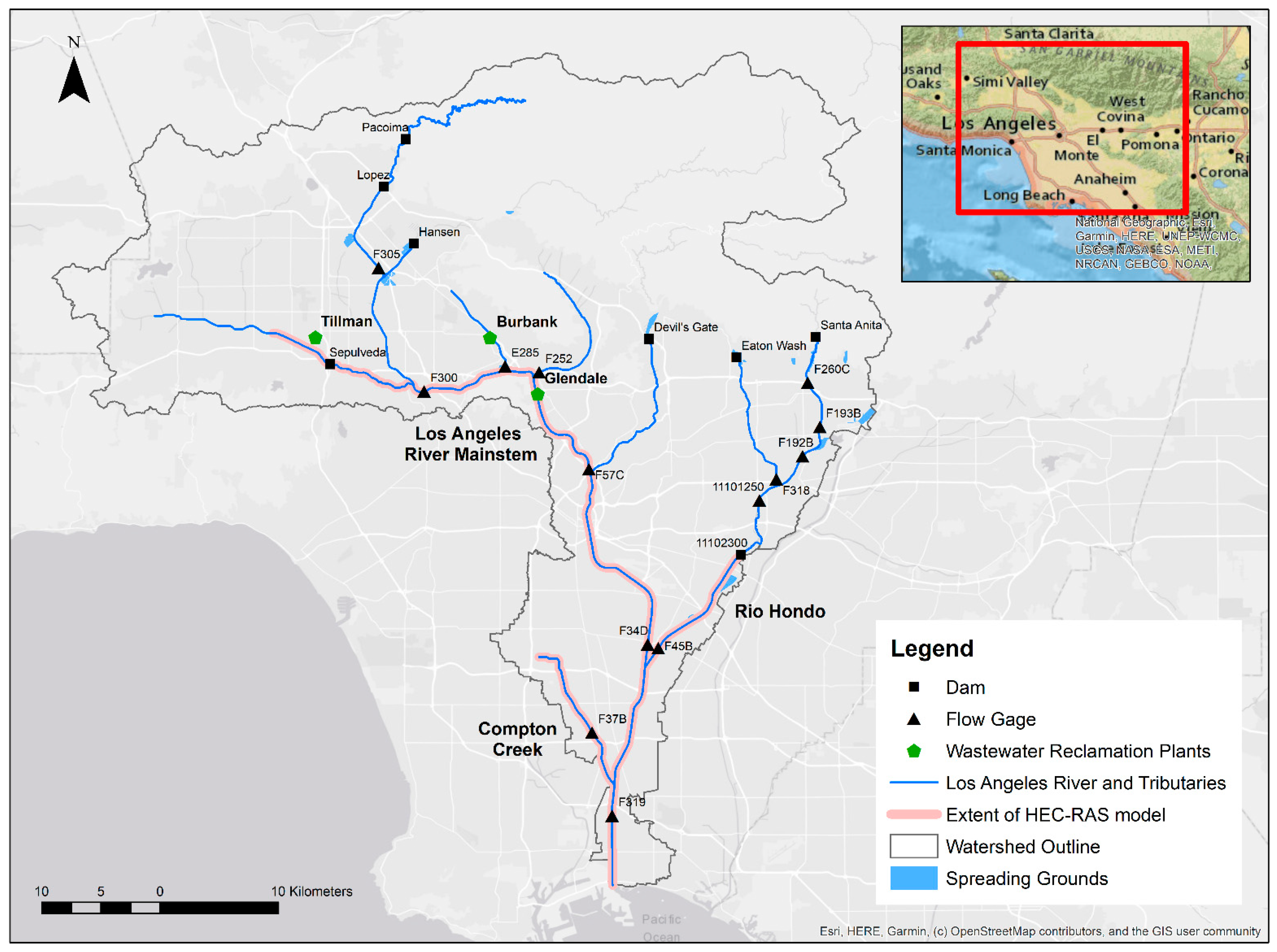
The tool was tested on a model of the Los Angeles River (73.8 km) and two tributaries, Rio Hondo (12.8 km) and Compton Creek (13.7 km; Figure 3 [33]). The Los Angeles River watershed is in Los Angeles County, CA, USA and is about 2160 km2. About 32% of the watershed is impervious and dominant land use types include residential, open space, and commercial. Slopes within the watershed vary from 20% in the northern national forest to 0.2% in the densely urbanized lower watershed (watershed average = 8%). The climate is characterized as Mediterranean with wet winters and dry summers. The average annual precipitation varies spatially in the catchment from about 200 to 460 mm (8 to 18 inches). The watershed is highly altered for water supply and flood control, and eight major dams are located within the watershed. Most of the mainstem river is channelized, and many of the channelized segments include a low flow channel (notch). Several spreading grounds are also operated within the watershed that capture stormwater, treated wastewater, or imported water to recharge groundwater aquifers. Three water reclamation plants (WRPs) are located within the watershed, which discharge a combined average of 2.1 m3/s (73 cfs) to the river annually, and contribute a significant amount of the dry season flow (Figure 3 [33]). The Los Angeles River watershed serves as an ideal case study because of the large range in channel geometries and flow rates within the system. The model used for the case study was too large to run in unsteady state without exceeding the maximum allowed error and therefore could not be calibrated using the built-in automatic calibration system in HEC-RAS.
The model was assembled from several partial models retrieved from local consultants and government agencies [34,35,36,37,38]. The model includes about 3000 nodes over both channelized and soft-bottomed portions of the Los Angeles River between the estuary and Sepulveda Dam, Compton Creek, and Rio Hondo up to Whittier Narrows Dam (Figure 3). Empirical data were available for several points throughout the system covering both rectangular and trapezoidal cross-sections, and some with a smaller low flow channel within the main channel. We used five flow gages for the case study (Figure 3):
- F37B, a rectangular cross-section in Compton Creek
- USGS 11102300, a trapezoidal cross-section in Rio Hondo
- F45B, a trapezoidal cross-section in Rio Hondo
- F300, a rectangular cross-section with a low-flow channel in the LA River mainstem
- F319, a trapezoidal cross-section with a low-flow channel in the LA River mainstem
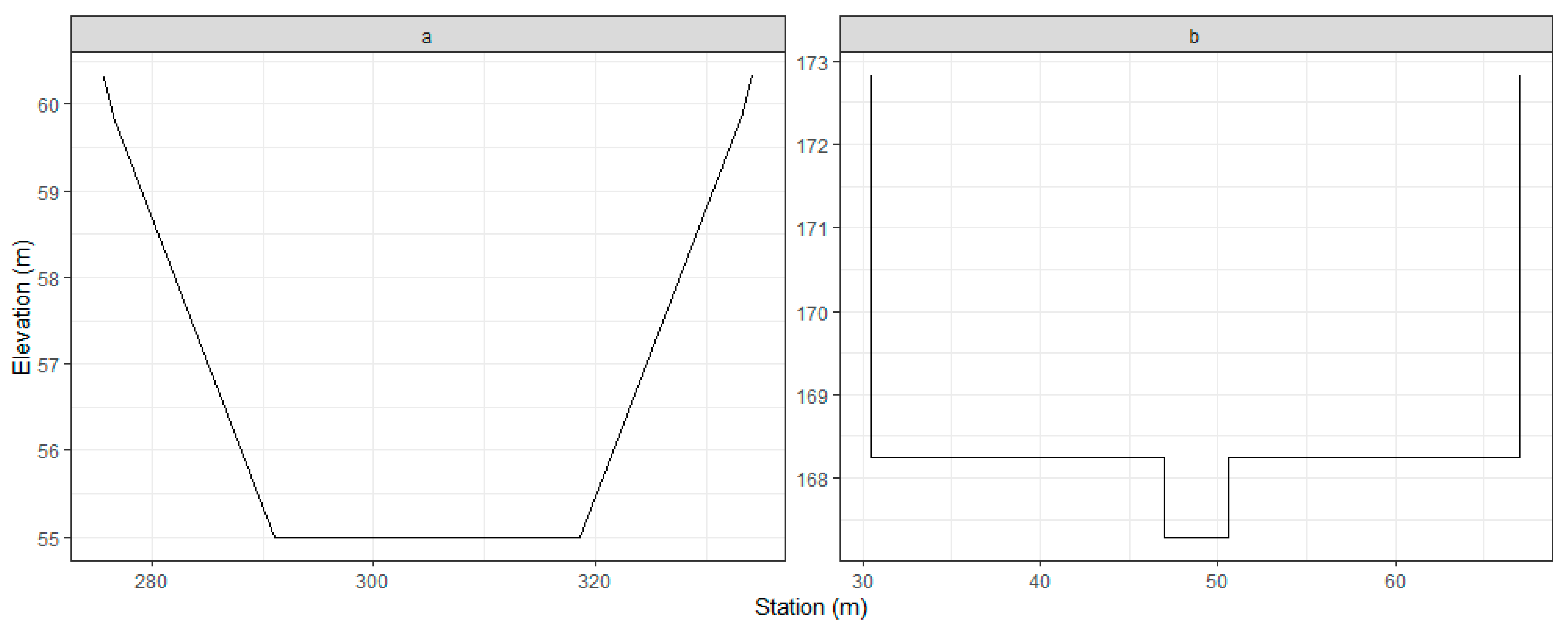
All calibration gages were in concrete channels. The data for the non-USGS (F-) gages were provided by Los Angeles County Department of Public Works, while the data for the USGS gage were retrieved from USGS Water Data for the Nation [22]. Two examples of channel cross-sections, including one with a low flow channel, are included in Figure 4. The empirical data include a wide range of discharge rates, ranging from less than 0.03 cms to greater than 300 cms (1–10,000 cfs). Automatic mode was used for all calibrations.
Based on general recommendations for model fitting [39], we selected RMSE and NSE for objective functions in Raspy-Cal, which are defined in Equations (1) and (2) below, respectively [39]. Reaches with low flow notches (e.g., F300 in Figure 4) were calibrated separately for low and high flows. To evaluate the performance of the automatic calibration algorithm, automatically calibrated roughness coefficients and rating curves were compared to those achieved with manual calibration.
where are the observed and modeled rating curve values, respectively, is the average observed value, n is the number of flow rates simulated, and is the standard deviation of the observed data.
3. Results and Discussion
3.1. User Interface
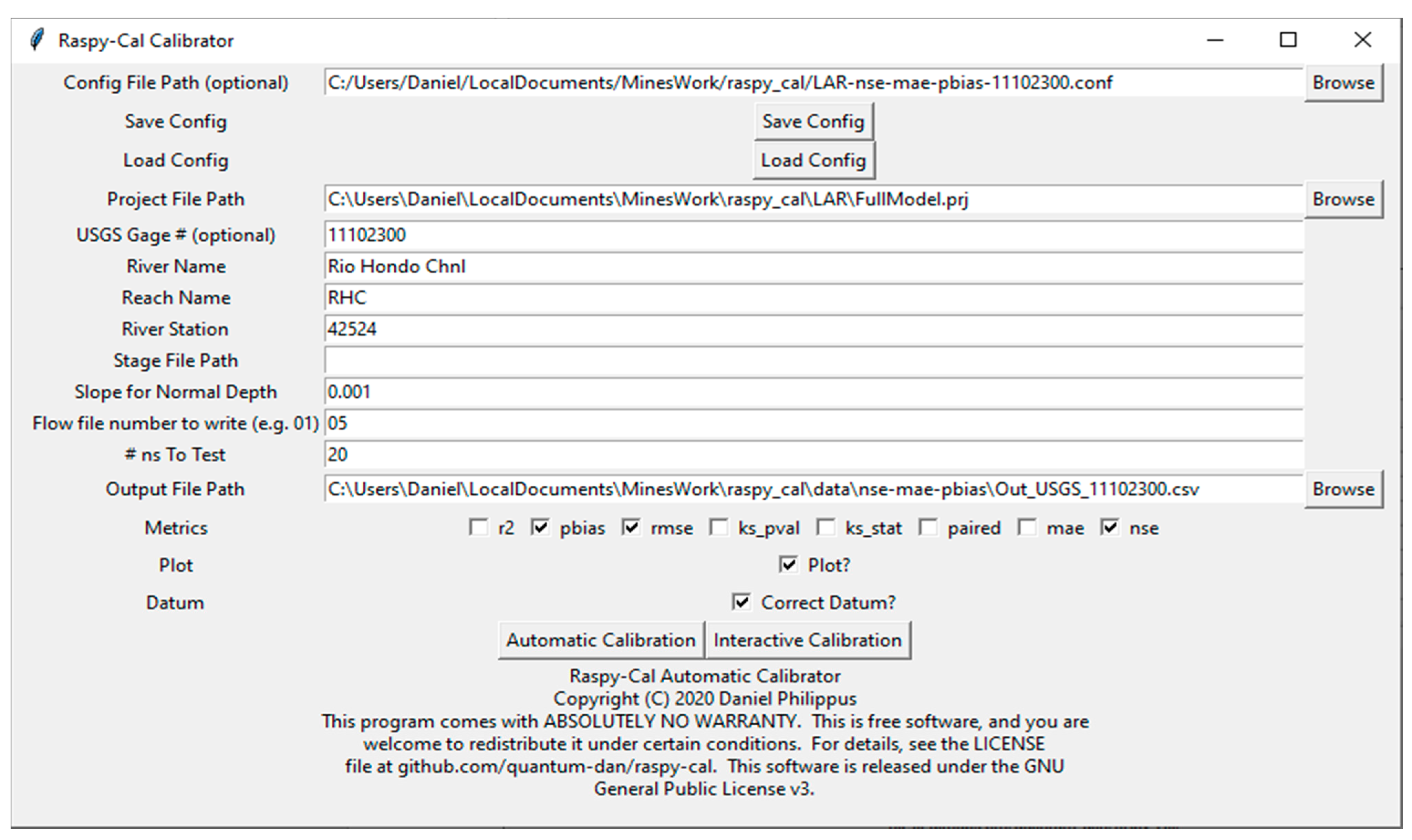
Raspy-Cal can be used either through the command line or through a graphical user interface. The command-line interface interactively requests any required information that is not provided by a configuration file. Figure 5 shows the graphical interface, which visually displays the fields that would be requested by the command-line interface and, after simulations, displays the results. The parameters can be specified interactively, or the user can load a configuration file containing information about how to run the simulation. The configuration file format is designed to be human-readable and -writable, consisting of “key:value” entries, and the graphical interface can also save the current settings to a configuration file. A configuration file that is entirely filled out will allow simulations to be run from the command line without any further input. With both interfaces, the results are displayed in the form of a table of roughness coefficients and fit metrics, as in Table 1, and a plot comparing empirical to simulated rating curves, as in Figure 6. Raspy-Cal also saves the metrics table and the raw data as a comma separated value file (.csv) and the plot as a PNG image. For testing purposes, a demo project is provided in Releases along with the Raspy-Cal executable, which is linked to from the Raspy-Cal website.
3.2. Case Study
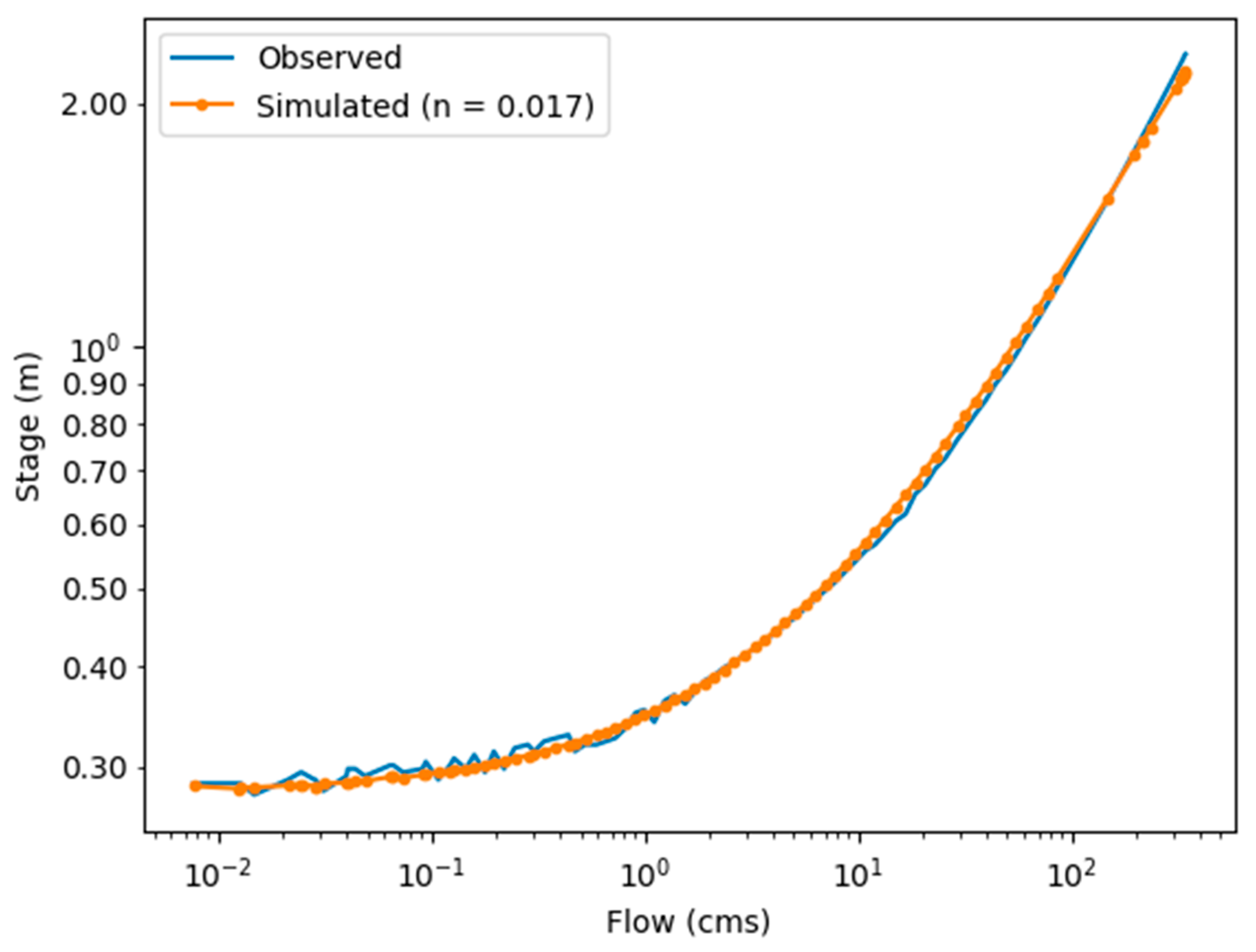
Raspy-Cal successfully calibrated most reaches of the model. An example of a good model fit is shown in Figure 7 for a concrete-lined cross section on the Rio Hondo Tributary (USGS 11102300), with an NSE of 0.971 and RMSE of 8.5 cm.
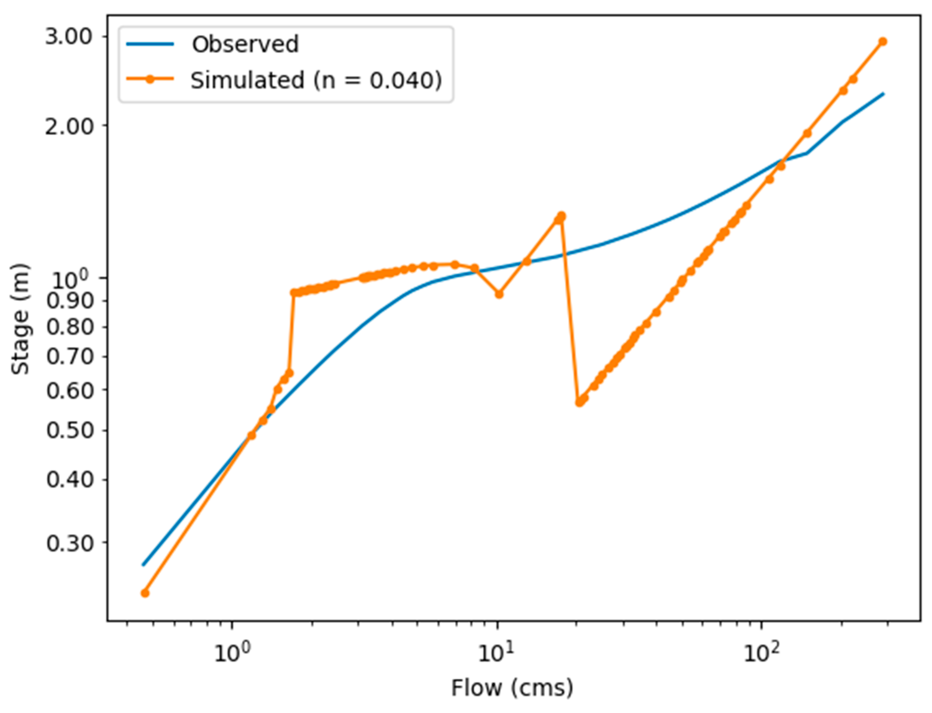
However, Raspy-Cal was unable to successfully calibrate Manning’s n for parts of the channel with highly irregular cross-sections (i.e., low-flow channels; see Figure 4 for the cross-section and Figure 8 for the result) when calibrating over the entire flow range. In this case, the tool fit the low flow section well but not the high flow section. On recalibrating separately for the low and high flow ranges, the calibration converged to roughness coefficients of 0.035 for low flows and 0.020 for high flows, both substantially different than the manually calibrated values of 0.020 for low flows and 0.008 for high flows. This is highlighted in the separate low-flow/high-flow plots along with several other case study locations in Figure 9.
Similar comparisons for each of the testing cross-sections are shown below in Table 2, and selected rating curve comparisons, covering rectangular, trapezoidal, and low-flow channels, are shown in Figure 9. The comparison is based on the rating curve plots for each case, as the automatic method, with sufficient trials, always converges on the set of optimal solutions for the specified fit coefficients; however, this would entirely miss, for example, the issues created by the low flow channel, where the optimal fit that attempts to apply a single roughness coefficient to all flow regimes is not in fact a very close fit. In each case, the automatic calibration results proved to be either comparable or a closer fit; in the case of the low-flow channel, this held true when running separate calibrations for low and high flows. The automatic calibrations generally took several hours to run 100 trials, which was a longer runtime than manual calibrations due to running more trials. However, the overall process involved much less time spent by the user because it could be run in the background until results were produced. As shown in Figure 9, in some cases datum adjustment was helpful for producing a good fit, whereas in others it caused a worse fit; as it is an optional adjustment, the user can determine if it is required for their particular application.
3.3. Discussion
In a few cases, the results of automatic calibration were much better than those of manual calibration; this was especially true in the case of the Upper LA River for low flows. In most cases where results were comparable, the automatic calibration retained a significant advantage in speed and convenience, as each calibration took several hours at most. This means that the entire river system could be calibrated in a few days, whereas calibrating the system manually took weeks. This corresponds to similar efforts for other models, which have often found heuristic algorithms to be an efficient way of accurately calibrating hydraulic and hydrologic models [12,41].
The cross-sections with a low-flow channel cause Manning’s equation to behave strangely around the transition from the low flow notch to the main channel due to a sudden increase in wetted perimeter without a significant corresponding increase in flow area (Figure 4). This facilitated testing the calibration tool to see how it would handle these more complex situations. It turned out to be necessary to calibrate separately for low and high flows; this had also been necessary with manual calibration. With this constraint, Raspy-Cal produced better results and did so more efficiently than manual calibration. We did not use interactive mode for the case study to test the genetic algorithm, but, for this and other more complex situations, the interactive option is useful to allow the modeler to apply their judgment, as has been implemented in other automatic calibration systems [42].
It is possible that the requirement to calibrate high flows and low flows separately is due to different roughness coefficients throughout the cross-section. Raspy-Cal does not currently support spatially-variable roughness, but this is a key planned usage improvement. In addition to support for roughness variation within cross-sections, integrated support for multi-cross-section calibration, allowing both faster overall calibration and automatic handling of longitudinal roughness variations, will be an important ease-of-use improvement. For maximum convenience, handling of HEC-RAS and Raspy-Cal errors and support for automatic validation will also be necessary.
3.4. Future Work
While NSGA-II is popular for multi-objective calibration, Lin et al. [12] have argued that equally effective and more efficient algorithms, namely dynamically-dimensioned search in their case, exist for the same purpose. Dynamically-dimensioned search was also chosen for the Soil and Water Assessment Tool (SWAT) Integrated Parameter Estimation and Uncertainty Analysis Tool Plus (IPEAT+) calibration utility because of its efficiency [43]. It would be worth comparing some such algorithms for efficiency and results, as an algorithm involving fewer iterations could result in being able to achieve the same accuracy much faster, or better accuracy through more detail in the same time. The architecture of the Raspy-Cal code also makes it easy to add new calibration algorithms, as the optimization algorithm portion is independent of other components. Lin et al. [12] also calibrated separately for low- and high-flow roughness coefficients, which would be a valuable feature for concerns such as low-flow channels. A further efficiency advantage could be possible through parallel computing, as in the example of Zhang et al. [44], which achieved speedups by a factor of up to 110 when using several dozen processor cores to calibrate a SWAT model in parallel.
A longer-term goal would be to make use of the tool’s intentionally generic architecture to extend it to other aspects of calibration within hydraulic and hydrologic modeling. This would require two steps: extending the options for calibration parameters and data comparison beyond roughness coefficient and stage, and developing Raspy-like wrappers for other models. For example, it would require minimal modification to use Raspy-Cal to provide extended calibration functionality, such as the use of NSGA-II, to HSPF by using the existing PyHSPF package [21] as an automation layer. Such development work is made easier by the open-source nature of the tool, as it makes it easy to see what is required of other interfaces as well as clearly showcasing what could be called the reference implementation, Raspy.
It would also be useful to have access to the libraries available in R, as in the example of Wu and Liu [45], which made use of a powerful R modeling framework to provide not just model fit optimization but also sensitivity analysis and other useful features. Being able to access HEC-RAS automation through R would also likely be easier for practitioners in the field, as R is well-known for its use in statistics and data analysis. This suggests the goal of providing an R interface to Raspy-Cal and Raspy, likely through the Reticulate library [46], which facilitates using Python from R.
4. Conclusions
Hydraulic modeling is a powerful tool and calibration of models is important to produce reliable results. However, this is often a time-consuming process when done manually, and no general, easy to use automatic calibration frameworks supporting the steady-state simulations necessary for large models currently exist for the HEC-RAS hydraulic modeling system. This work presents an easy to use, general automatic calibration tool for HEC-RAS as well as a case study of its use.
Several important usability improvements remain: support for longitudinal and within-cross-section roughness variations; integrated error handling; and automatic validation. These changes are planned for implementation during continuing development. The present state of development, however, is fully usable and provides advantages compared to manual calibration. Results from the case study in the Los Angeles River watershed indicate that automatic calibration with the developed tool improves calibration statistics and increases efficiency.
Author Contributions
Conceptualization, D.P., J.M.W., R.A. and T.S.H.; Software, D.P.; Investigation, D.P.; Writing—original draft, D.P.; Writing—review and editing, D.P., J.M.W., R.A. and T.S.H. All authors have read and agreed to the published version of the manuscript.
Funding
This research was principally funded by the City of Los Angeles, Department of Water and Power (DWP) and Bureau of Sanitation (BoS). Additional funding was provided by Los Angeles County Public Works (LADPW), Los Angeles County Flood Sanitation Districts (LACSD), the Watershed Conservation Authority (WCA), a joint powers authority between the Rivers and Mountains Conservancy (RMC) and the Los Angeles County Flood Control District, and the Mountains Recreation and Conservation Authority (MRCA), a joint power of the Santa Monica Mountains Conservancy, the Conejo Recreation and Park District and the Ranch Simi Recreation and Park District.
Data Availability Statement
The Python code presented in this study is openly available in GitHub at github.com/quantum-dan/raspy-cal, github.com/quantum-dan/raspy, and github.com/larflows/pyrasfile (accessed on 26 September 2021). The hydraulic model used for the case study is available upon reasonable request.
Acknowledgments
This project was conducted through a collaboration with the Southern California Coastal Water Research Project (SCCWRP), the State Water Resources Control Board, the Los Angeles Regional Water Quality Control Board, and local municipalities and stakeholders. We thank all members of the Stakeholder Workgroup and the Technical Advisory Group who provided critical input, advice, and review over the course of this project. Additional project information is available at https://www.waterboards.ca.gov/water_issues/programs/larflows.html and https://www.sccwrp.org/about/research-areas/ecohydrology/los-angeles-river-flows-project/ (accessed on 26 September 2021).
Conflicts of Interest
The authors declare no conflict of interest.
References
- Abdi, R.; Endreny, T.; Nowak, D. A model to integrate urban river thermal cooling in river restoration. J. Environ. Manag. 2020, 258, 110023. [Google Scholar] [CrossRef]
- Papadaki, C.; Bellos, V.; Stoumboudi, M.; Kopsiaftis, G.; Dimitriou, E. Evaluation of streamflow habitat relationships using habitat suitability curves and HEC-RAS. Eur. Water 2017, 58, 127–134. [Google Scholar]
- Shafroth, P.B.; Wilcox, A.C.; Lytle, D.A.; Hickey, J.T.; Andersen, D.C.; Beauchamp, V.B.; Hautzinger, A.; McMullen, L.E.; Warner, A. Ecosystem effects of environmental flows: Modelling and experimental floods in a dryland river. Freshw. Biol. 2010, 55, 68–85. [Google Scholar] [CrossRef]
- US Army Corps of Engineers. HEC-RAS. 2019. Available online: https://www.hec.usace.army.mil/software/hec-ras/ (accessed on 4 March 2020).
- US Army Corps of Engineers. HEC-RAS Features. 2019. Available online: https://www.hec.usace.army.mil/software/hec-ras/features.aspx (accessed on 4 March 2020).
- Abbas, S.A.; Al-Aboodi, A.H.; Ibrahim, H.T. Identification of Manning’s Coefficient Using HEC-RAS Model: Upstream Al-Amarah Barrage. J. Eng. 2020, 2020, 6450825. [Google Scholar] [CrossRef] [Green Version]
- Ardıçlıoğlu, M.; Kuriqi, A. Calibration of channel roughness in intermittent rivers using HEC-RAS model: Case of Sarimsakli creek, Turkey. SN Appl. Sci. 2019, 1, 1–9. [Google Scholar] [CrossRef] [Green Version]
- Parhi, P.K.; Sankhua, R.N.; Roy, G.P. Calibration of Channel Roughness for Mahanadi River, (India) Using HEC-RAS Model. J. Water Resour. Prot. 2012, 4, 847–850. [Google Scholar] [CrossRef] [Green Version]
- Alamdari, N.; Sample, D.J. A multiobjective simulation-optimization tool for assisting in urban watershed restoration planning. J. Clean. Prod. 2019, 213, 251–261. [Google Scholar] [CrossRef]
- Bekele, E.G.; Nicklow, J.W. Multi-objective automatic calibration of SWAT using NSGA-II. J. Hydrol. 2007, 341, 165–176. [Google Scholar] [CrossRef]
- Eckhardt, K.; Arnold, J.G. Automatic calibration of a distributed catchment model. J. Hydrol. 2001, 251, 103–109. [Google Scholar] [CrossRef]
- Lin, F.R.; Wu, N.J.; Tu, C.H.; Tsay, T.K. Automatic Calibration of an Unsteady River Flow Model by Using Dynamically Dimensioned Search Algorithm. Math. Probl. Eng. 2017, 2017, 7919324. [Google Scholar] [CrossRef]
- Seong, C.; Her, Y.; Benham, B.L. Automatic Calibration Tool for Hydrologic Simulation Program-FORTRAN Using a Shuffled Complex Evolution Algorithm. Water 2015, 7, 503–527. [Google Scholar] [CrossRef] [Green Version]
- Goodell, C. Breaking the HEC-RAS Code: A User’s Guide to Automating HEC-RAS; h2ls: Portland, OR, USA, 2014. [Google Scholar]
- Leon, A.S.; Goodell, C. Controlling HEC-RAS using MATLAB. Environ. Model. Softw. 2016, 84, 339–348. [Google Scholar] [CrossRef] [Green Version]
- Dysarz, T. Application of Python Scripting Techniques for Control and Automation of HEC-RAS Simulations. Water 2018, 10, 1382. [Google Scholar] [CrossRef] [Green Version]
- Timbadiya, P.V.; Patel, P.L.; Porey, P.D.; Timbadiya, P.V.; Patel, P.L.; Porey, P.D. Calibration of HEC-RAS Model on Prediction of Flood for Lower Tapi River, India. J. Water Resour. Prot. 2011, 3, 805–811. [Google Scholar] [CrossRef] [Green Version]
- Peña-Castellanos, G. PyRAS·PyPI. 2015. Available online: https://pypi.org/project/PyRAS/ (accessed on 23 January 2020).
- US Army Corps of Engineers. HEC-RAS User’s Manual. December 2020. Available online: https://www.hec.usace.army.mil/software/hec-ras/documentation/HEC-RAS_6.0_Users_Manual.pdf (accessed on 18 January 2021).
- Deb, K.; Pratap, A.; Agarwal, S.; Meyarivan, T. A fast and elitist multiobjective genetic algorithm: NSGA-II. IEEE Trans. Evol. Comput. 2002, 6, 182–197. [Google Scholar] [CrossRef] [Green Version]
- Lampert, D.J.; Wu, M. Automated Approach for Construction of Long-Term, Data-Intensive Watershed Models. J. Comput. Civ. Eng. 2018, 32, 06018001. [Google Scholar] [CrossRef]
- USGS. USGS Water Data for the Nation. 2020. Available online: https://waterdata.usgs.gov/nwis (accessed on 4 March 2020).
- Moriasi, D.N.; Arnold, J.G.; van Liew, M.W.; Bingner, R.L.; Harmel, R.D.; Veith, T.L. Model evaluation guidelines for systematic quantification of accuracy in watershed simulations. Trans. ASABE 1983, 50, 885–900. [Google Scholar] [CrossRef]
- Hsu, H.; Lachenbruch, P.A. Paired t Test. In Encyclopedia of Biostatistics; John Wiley & Sons, Ltd.: Chichester, UK, 2005. [Google Scholar] [CrossRef]
- Massey, F.J. The Kolmogorov-Smirnov Test for Goodness of Fit. J. Am. Stat. Assoc. 1951, 46, 68–78. [Google Scholar] [CrossRef]
- Roberts, W.; Williams, G. HydroErr·PyPI. 2019. Available online: https://pypi.org/project/HydroErr/ (accessed on 4 March 2020).
- Virtanen, P.; Gommers, R.; Oliphant, T.E.; Haberland, M.; Reddy, T.; Cournapeau, D.; Burovski, E.; Peterson, P.; Weckesser, W.; Bright, J.; et al. SciPy 1.0: Fundamental Algorithms for Scientific Computing in Python. Nat. Methods 2020, 17, 261–272. [Google Scholar] [CrossRef] [PubMed] [Green Version]
- Zambrano-Bigiarini, M. hydroGOF package|R Documentation. 2020. Available online: https://www.rdocumentation.org/packages/hydroGOF/versions/0.3-10 (accessed on 4 March 2020).
- Hunter, J.D. Matplotlib: A 2D Graphics Environment. Comput. Sci. Eng. 2007, 9, 90–95. [Google Scholar] [CrossRef]
- Cheng, M.-Y.; Prayogo, D.; Wu, Y.-W. Novel Genetic Algorithm-Based Evolutionary Support Vector Machine for Optimizing High-Performance Concrete Mixture. J. Comput. Civ. Eng. 2013, 28, 06014003. [Google Scholar] [CrossRef] [Green Version]
- Shukla, P.K.; Deb, K.; Tiwari, S. Comparing Classical Generating Methods with an Evolutionary Multi-objective Optimization Method. Lect. Notes Comput. Sci. 2005, 3410, 311–325. [Google Scholar] [CrossRef]
- Hadka, D. Platypus-Opt·PyPI. 2018. Available online: https://pypi.org/project/Platypus-Opt/ (accessed on 4 March 2020).
- Read, L.K.; Hogue, T.S.; Edgley, R.; Mika, K.; Gold, M. Evaluating the Impacts of Stormwater Management on Streamflow Regimes in the Los Angeles River. J. Water Resour. Plan. Manag. 2019, 145, 05019016. [Google Scholar] [CrossRef]
- US Army Corps of Engineers. HEC-RAS Model for Stormwater Management Plan; US Army Corps of Engineers: Los Angeles, CA, USA, 2004. [Google Scholar]
- HDR CDM. HEC-RAS Model for San Gabriel River, San Jose Creek, Compton Creek, Upper Rio Hondo, Coyote Creek, Verdugo Wash, Arroyo Seco; HDR CDM: Irvine, CA, USA, 2011. [Google Scholar]
- US Army Corps of Engineers. HEC-RAS Model for Upper Los Angeles River and Tujunga Wash; US Army Corps of Engineers: Los Angeles, CA, USA, 2005. [Google Scholar]
- Environmental Science Associates. HEC-RAS Model for Glendale 2018 Wastewater Change Petition; Environmental Science Associates: Los Angeles, CA, USA, 2018. [Google Scholar]
- Los Angeles Department of Public Works, Los Angeles County Flood Control. 2011. Available online: https://dpw.lacounty.gov/lacfcd/WDR/fs.aspx (accessed on 4 March 2020).
- Ritter, A.; Muñoz-Carpena, R. Performance evaluation of hydrological models: Statistical significance for reducing subjectivity in goodness-of-fit assessments. J. Hydrol. 2013, 480, 33–45. [Google Scholar] [CrossRef]
- Chin, D.A. Water-Resources Engineering, 3rd ed.; Pearson: Upper Saddle River, NJ, USA, 2013. [Google Scholar]
- Bekele, E.G.; Nicklow, J.W. Evolutionary Algorithms for Multi-Objective, Automatic Calibration of a Semi-Distributed Hydrologic Model. In Proceedings of the World Environmental and Water Resource Congress 2006, Omaha, NE, USA, 21–25 May 2006; pp. 1–12. [Google Scholar] [CrossRef]
- Borthwick, M.F.; Packham, I.S.; Rafiq, M.Y. Interactive Visualization for Evolutionary Optimization of Conceptual Rainfall-Streamflow Models. J. Comput. Civ. Eng. 2008, 22, 40–49. [Google Scholar] [CrossRef]
- Yen, H.; Park, S.; Arnold, J.G.; Srinivasan, R.; Chawanda, C.J.; Wang, R.; Feng, Q.; Wu, J.; Miao, C.; Bieger, K.; et al. IPEAT+: A Built-In Optimization and Automatic Calibration Tool of SWAT+. Water 2019, 11, 1681. [Google Scholar] [CrossRef] [Green Version]
- Zhang, X.; Beeson, P.; Link, R.; Manowitz, D.; Izaurralde, R.C.; Sadeghi, A.; Thomson, A.M.; Sahajpal, R.; Srinivasan, R.; Arnold, J.G. Efficient multi-objective calibration of a computationally intensive hydrologic model with parallel computing software in Python. Environ. Model. Softw. 2013, 46, 208–218. [Google Scholar] [CrossRef]
- Wu, Y.; Liu, S. Automating calibration, sensitivity and uncertainty analysis of complex models using the R package Flexible Modeling Environment (FME): SWAT as an example. Environ. Model. Softw. 2012, 31, 99–109. [Google Scholar] [CrossRef]
- Tang, Y.; Eddelbuettel, D.; Lewis, B.; Keydana, S.; Hafen, R.; Geelnard, M. Reticulate; RStudio: Boston, MA, USA, 2020. [Google Scholar]
Figure 1.
Raspy-Cal and Raspy architecture. PyRASFile is a set of HEC-RAS file writers and parsers for Python. The unified API class within Raspy provides a unified, abstract interface for other programs (e.g., Raspy-Cal) to use.
Figure 1.
Raspy-Cal and Raspy architecture. PyRASFile is a set of HEC-RAS file writers and parsers for Python. The unified API class within Raspy provides a unified, abstract interface for other programs (e.g., Raspy-Cal) to use.

Figure 2.
Process diagram for Raspy-Cal. The interface collects general information such as the project file, number of Manning’s n coefficients to test, whether to plot, and empirical data and either runs in interactive or automatic mode. Results are a table of metrics with nondominated results and, if specified, rating curves.

Figure 3.
Map of the Los Angeles River watershed and extent of the HEC-RAS model.

Figure 4.
Two example cross-sections, (a) for a node within Rio Hondo (USGS 11102300, left) and (b) for a node within the mainstem of the Los Angeles River with a low-flow channel (F300, right).
Figure 4.
Two example cross-sections, (a) for a node within Rio Hondo (USGS 11102300, left) and (b) for a node within the mainstem of the Los Angeles River with a low-flow channel (F300, right).

Figure 5.
Raspy-Cal graphical user interface. Note that settings are specific to the given calibration reach. Also note that the calibration river station must be a cross-section, not a hydraulic structure.
Figure 5.
Raspy-Cal graphical user interface. Note that settings are specific to the given calibration reach. Also note that the calibration river station must be a cross-section, not a hydraulic structure.

Figure 6.
Raspy-Cal output that compares simulated with observed rating curves for demo project cross-section 900.00*. Note log scale due to large range in flow regime in some systems.
Figure 6.
Raspy-Cal output that compares simulated with observed rating curves for demo project cross-section 900.00*. Note log scale due to large range in flow regime in some systems.

Figure 7.
Example of a good rating curve comparison from Raspy-Cal for the Los Angeles River, Los Angeles County, CA, USA. Plot shows a trapezoidal, concrete-lined portion of the channel (USGS 11102300; right).
Figure 7.
Example of a good rating curve comparison from Raspy-Cal for the Los Angeles River, Los Angeles County, CA, USA. Plot shows a trapezoidal, concrete-lined portion of the channel (USGS 11102300; right).

Figure 8.
Example of a poor rating curve comparison from Raspy-Cal for the Los Angeles River, Los Angeles County, CA, USA. Plot shows a cross section with a low flow channel (F300).
Figure 8.
Example of a poor rating curve comparison from Raspy-Cal for the Los Angeles River, Los Angeles County, CA, USA. Plot shows a cross section with a low flow channel (F300).

Figure 9.
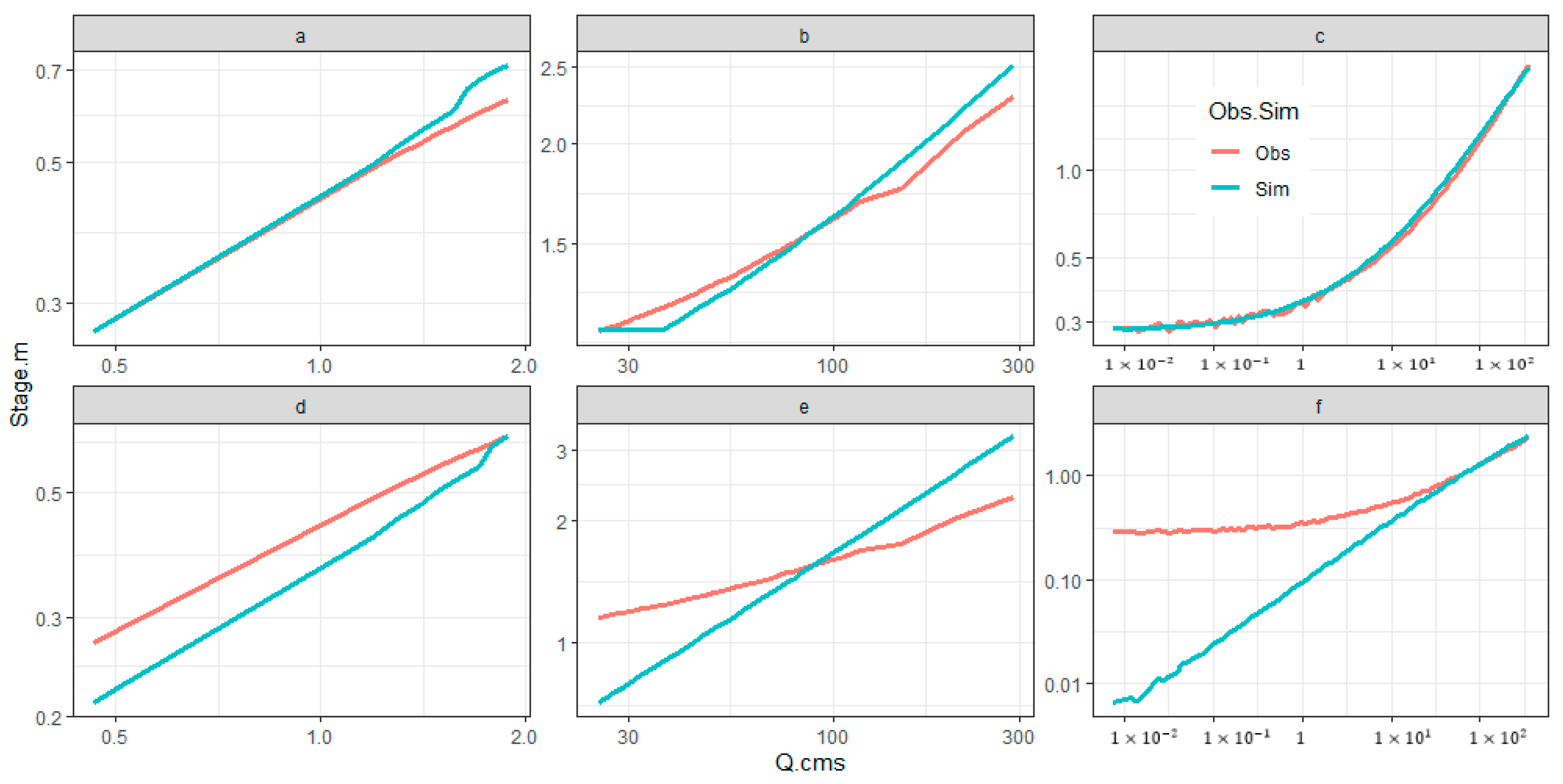
Selected rating curve comparisons for (a) LA River (F300) at low flows with datum adjustment, (b) LA River (F300) at high flows with datum adjustment, (c) Rio Hondo (USGS 11102300) with datum adjustment, (d) LA River (F300) at low flows without datum adjustment, (e) LA River (F300) at high flows without datum adjustment, and (f) Rio Hondo (USGS 11102300) without datum adjustment. In some cases, calibration is more successful with datum adjustment, as for USGS 11102300 and F300 (high flows) (panels (b,c)); in others, it produces a better apparent fit but unrealistic result, as with F300 (low flows) (panel (a)), where the datum-adjusted calibration resulted in n = 0.292 for a concrete channel (typical roughness coefficients for concrete are between 0.011 and 0.020 [40]). In such cases, unadjusted calibration tends to produce more realistic results, although the apparent fit does not tend to be as good; datum adjustment should therefore only be used when the user is confident there is an actual datum gap.
Figure 9.
Selected rating curve comparisons for (a) LA River (F300) at low flows with datum adjustment, (b) LA River (F300) at high flows with datum adjustment, (c) Rio Hondo (USGS 11102300) with datum adjustment, (d) LA River (F300) at low flows without datum adjustment, (e) LA River (F300) at high flows without datum adjustment, and (f) Rio Hondo (USGS 11102300) without datum adjustment. In some cases, calibration is more successful with datum adjustment, as for USGS 11102300 and F300 (high flows) (panels (b,c)); in others, it produces a better apparent fit but unrealistic result, as with F300 (low flows) (panel (a)), where the datum-adjusted calibration resulted in n = 0.292 for a concrete channel (typical roughness coefficients for concrete are between 0.011 and 0.020 [40]). In such cases, unadjusted calibration tends to produce more realistic results, although the apparent fit does not tend to be as good; datum adjustment should therefore only be used when the user is confident there is an actual datum gap.


Table 1.
Sample Raspy-Cal output table.
| Roughness Coefficient | R2 | RMSE (m) | NSE |
|---|---|---|---|
| 0.094 | 0.984 | 0.29 | 0.514 |
| 0.106 | 0.982 | 0.247 | 0.647 |
| 0.128 | 0.98 | 0.162 | 0.847 |
| 0.139 | 0.979 | 0.122 | 0.913 |
| 0.15 | 0.975 | 0.093 | 0.95 |
Table 2.
Comparison of automatic and manual calibration results for all calibration cross-sections.
| Description | Gage ID | Manning’s n | NSE | RMSE (cm) | |||
|---|---|---|---|---|---|---|---|
| Automatic | Manual | Automatic | Manual | Automatic | Manual | ||
| Rio Hondo below Whittier Narrows Dam | 11102300 | 0.017 | 0.014 | 0.997 | 0.996 | 3.4 | 3.5 |
| Rio Hondo below spreading grounds | F45B | 0.016 | 0.014 | 0.989 | 0.983 | 1.9 | 2.4 |
| Compton Creek | F37B | 0.016 | 0.010 | 0.985 | 0.838 | 2.2 | 7.2 |
| Los Angeles River above confluence with Burbank Channel–Low Flows | F300 | 0.035 | 0.02 | 0.890 | −1.28 | 3.2 | 14.3 |
| Los Angeles River above confluence with Burbank Channel–High Flows | F300 | 0.020 | 0.008 | 0.933 | 0.888 | 6.8 | 8.6 |
| Los Angeles River near above tidal reach | F319 | 0.013 | 0.012 | 0.995 | 0.989 | 2.5 | 3.7 |
Publisher’s Note: MDPI stays neutral with regard to jurisdictional claims in published maps and institutional affiliations. |
© 2021 by the authors. Licensee MDPI, Basel, Switzerland. This article is an open access article distributed under the terms and conditions of the Creative Commons Attribution (CC BY) license (https://creativecommons.org/licenses/by/4.0/).
Share and Cite
MDPI and ACS Style
Philippus, D.; Wolfand, J.M.; Abdi, R.; Hogue, T.S. Raspy-Cal: A Genetic Algorithm-Based Automatic Calibration Tool for HEC-RAS Hydraulic Models. Water 2021, 13, 3061. https://doi.org/10.3390/w13213061
AMA Style
Philippus D, Wolfand JM, Abdi R, Hogue TS. Raspy-Cal: A Genetic Algorithm-Based Automatic Calibration Tool for HEC-RAS Hydraulic Models. Water. 2021; 13(21):3061. https://doi.org/10.3390/w13213061
Chicago/Turabian StylePhilippus, Daniel, Jordyn M. Wolfand, Reza Abdi, and Terri S. Hogue. 2021. "Raspy-Cal: A Genetic Algorithm-Based Automatic Calibration Tool for HEC-RAS Hydraulic Models" Water 13, no. 21: 3061. https://doi.org/10.3390/w13213061
Note that from the first issue of 2016, this journal uses article numbers instead of page numbers. See further details here.