
Hydrogeochemical Characterization and Its Seasonal Changes of Groundwater Based on Self-Organizing Maps


1
State Key Laboratory of Water Cycle Simulation and Regulation, China Institute of Water Resources and Hydropower Research, Beijing 100038, China
2
School of Water Resources and Environment, China University of Geosciences, Beijing 100083, China
*
Author to whom correspondence should be addressed.
Water 2021, 13(21), 3065; https://doi.org/10.3390/w13213065
Submission received: 14 October 2021
/
Revised: 27 October 2021
/
Accepted: 30 October 2021
/
Published: 2 November 2021
(This article belongs to the Section Hydrogeology)
Abstract
:Water resources are scarce in arid or semiarid areas; groundwater is an important water source to maintain residents’ lives and the social economy; and identifying the hydrogeochemical characteristics of groundwater and its seasonal changes is a prerequisite for sustainable use and protection of groundwater. This study takes the Hongjiannao Basin as an example, and the Piper diagram, the Gibbs diagram, the Gaillardet diagram, the Chlor-alkali index, the saturation index, and the ion ratio were used to analyze the hydrogeochemical characteristics of groundwater. Meanwhile, based on self-organizing maps (SOM), quantification error (QE), topological error (TE), and the K-means algorithm, groundwater chemical data analysis was carried out to explore its seasonal variability. The results show that (1) the formation of groundwater chemistry in the study area was controlled by water–rock interactions and cation exchange, and the hydrochemical facies were HCO3-Ca type, HCO3-Na type, and Cl-Na type. (2) Groundwater chemical composition was mainly controlled by silicate weathering and carbonate dissolution, and the dissolution of halite, gypsum, and fluorite dominated the contribution of ions, while most dolomite and calcite were in a precipitated state or were reactive minerals. (3) All groundwater samples in wet and dry seasons were divided into five clusters, and the hydrochemical facies of clusters 1, 2, and 3 were HCO3-Ca type; cluster 4 was HCO3-Na type; and cluster 5 was Cl-Na type. (4) Thirty samples changed in the same clusters, and the groundwater chemistry characteristics of nine samples showed obvious seasonal variability, while the seasonal changes of groundwater hydrogeochemical characteristics were not significant.
1. Introduction
Groundwater plays a crucial role in domestic and irrigation activities in arid–semiarid regions where surface water resources are short in supply or low in quality [1,2,3]. Rapid urban and industrial growth has led to overexploitation of groundwater, causing increasingly prominent water-related problems (e.g., depletion of water resources accompanied by groundwater pollution) in local areas [4,5]. Hydrogeochemical analysis of groundwater is an important aspect of hydrogeological research, as it guides the sustainable use and managementof groundwater resources as well as ecological and environmental protection [6,7,8]. Hence, there is an urgent need to determine the characteristics and seasonal variability of the hydrogeochemical composition of regional groundwater to guide the implementation of management measures for groundwater resources and prevent their further deterioration.
The Hongjiannao Lake Basin is located at the eastern margin of the Cretaceous basin on the Ordos Plateau. Over the past two decades, unreasonable development and utilization of water resources, as well as frequent anthropogenic engineering activities have reduced the quality of water in the Hongjiannao Lake and caused ecological and environmental damage to the area [9,10,11]. Quaternary and Cretaceous groundwater discharge in the lake basin recharges and conserves Hongjiannao Lake. Groundwater is an important source of water that supports domestic and socioeconomic activities in this area [12,13]. Studies have tended to focus on the interpretation of the surface of the Hongjiannao Lake and its natural and anthropogenic influencing factors, as well as the flora and fauna resources in the Hongjiannao wetlands [14,15,16], while few have examined this area from a hydrogeological perspective [17]. No studies on the characteristics and seasonal variability of the hydrogeochemical composition of the groundwater in this lake basin have been reported.
Cluster analysis is a widely used, practical tool for studying the hydrogeochemical characteristics of groundwater [7,18]. Common clustering methods include principal component analysis, hierarchical cluster analysis, and k-means clustering. They can be employed to cluster samples of groundwater to characterize and assess its quality and to determine its hydrochemical characteristics [19,20,21]. Self-organizing maps (SOMs) can map complex high-dimensional data onto low-dimensional spaces to enable their visualization, based on the principle of competitive learning in artificial neural networks [22,23,24]. A SOM assigns samples with similar characteristics to one cluster while preserving their initial topological relationships. In other words, this technique places similar samples in one cluster and dissimilar samples in different clusters [25]. SOM-based clustering has been applied to the hydrogeochemical analysis and quality assessment of groundwater. Some researchers have noted that the selection of a suitable neuron size is the key to SOM-based clustering and have provided helpful theoretical guidance [20,21,26].
In this study, the hydrogeochemical characteristics of the groundwater in the Hongjiannao Lake Basin were determined by analyzing samples collected during the rainy and dry seasons using techniques such as Piper, Gibbs, and Gaillardet diagrams; the chloro-alkaline indices (CAIs); the saturation index (SI); and ion ratio analysis. The seasonal variability of the hydrogeochemical characteristics of the groundwater in the study area was determined through correlation and cluster analysis of its hydrochemical parameters using SOMs, the quantization error (QE), the topological error (TE), and k-means clustering. The research approach introduced in this study can provide theoretical and technical support for investigating the seasonal variability of the hydrogeochemical characteristics of groundwater in similar areas.
2. Description of the Study Area
2.1. Study Location and Climate
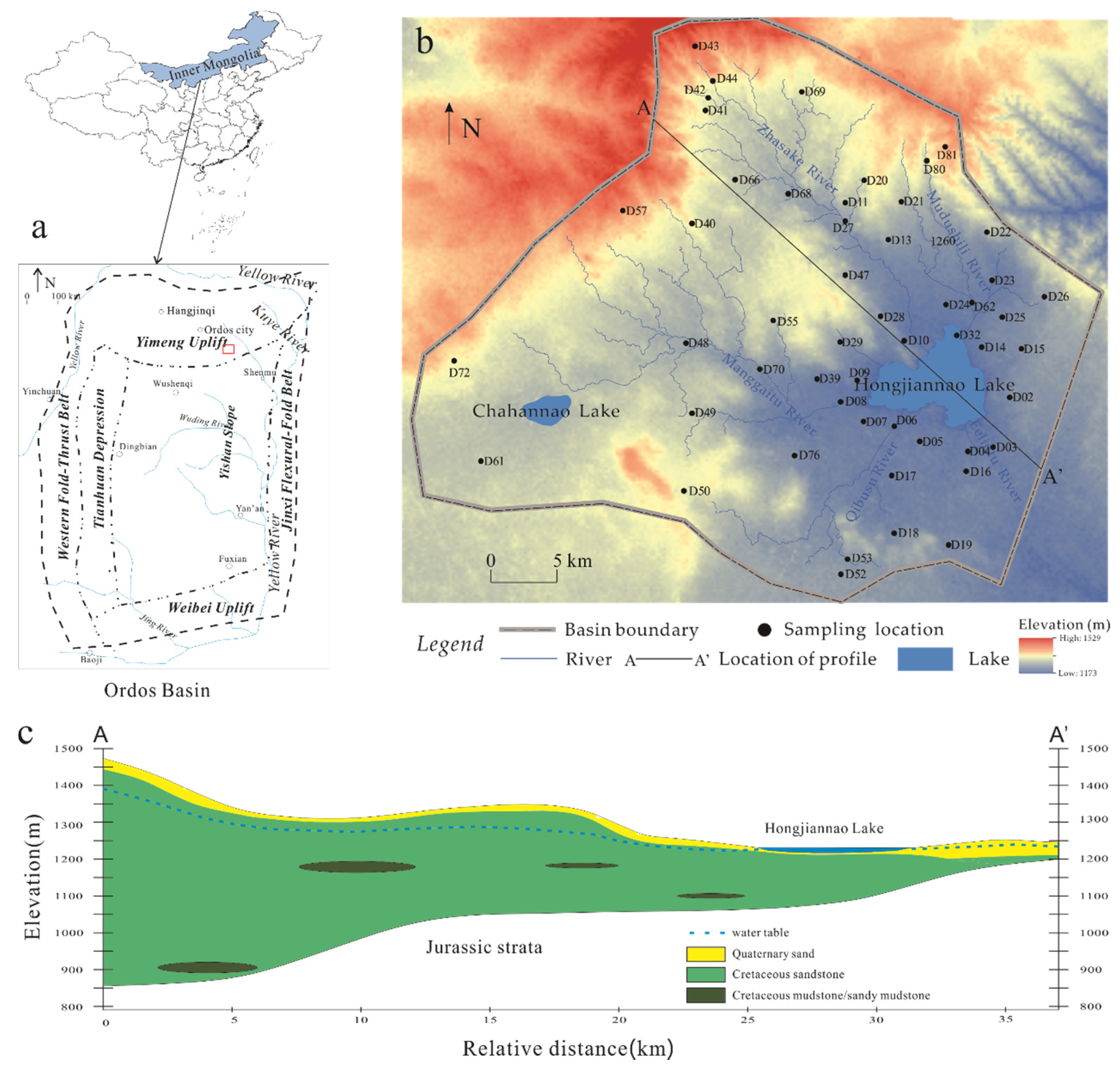
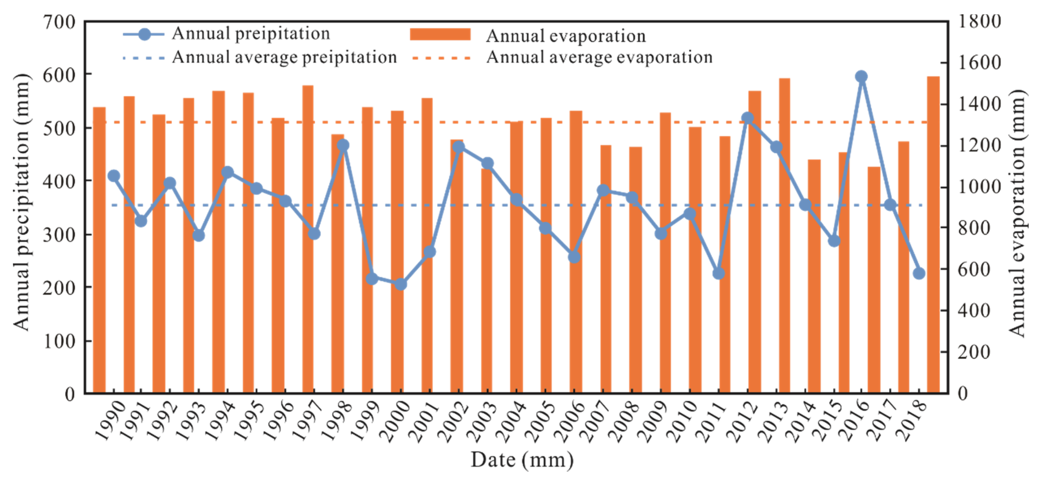
Encompassing an area of approximately 1440 km2, the Hongjiannao Lake Basin lies at the eastern margin of the Maowusu Desert and the junction of Shaanxi and Inner Mongolia (Figure 1). Located in a relatively low-lying area of the Maowusu Desert, Hongjiannao Lake is the largest desert freshwater lake in China, with a surface area of approximately 38 km2. The Hongjiannao Lake Basin has an arid–semiarid temperate plateau continental climate. Analysis of the variation in annual precipitation and evaporation in this area from 1990–2018 revealed the following. The multi-year annual average precipitation was 356.4 mm. Annually, most precipitation (69% of the total annual precipitation) fell in July through September (Figure 2), mainly in the form of rainstorms and with a maximum monthly precipitation of 223.7 mm, which tended to cause flooding. Evaporation peaked in April and then gradually decreased each month until October when it rebounded slightly. The multiyear maximum monthly evaporation was 258.1 mm, while the multiyear annual average evaporation was 1328.5 mm (measured with evaporating dishes with a diameter of 20 cm).
2.2. Hydrogeological Setting
The distribution and characteristics of the groundwater in the Hongjiannao Lake Basin are controlled primarily by factors such as the terrain, landforms, lithology, geological structures, and climatic conditions. Based on the type of water-bearing rock, the groundwater in this area can be categorized into pore water in loose rocks and pore-fissure water (PFW) in clastic rocks. (1) There are three main loose rock formations that contain pore water. (i) There are the phreatic pore water (PPW)–bearing quaternary–Holocene alluvial and diluvial formations. Distributed in a wide-valley banded pattern in the riverbeds and terraces in the gullies across the lake basin, this formation contains PPW and has a lithology composed mainly of gravelly, medium- to fine-grained sand with gravel and pebble layers at the bottom. (ii) There are PPW-bearing quaternary–Holocene aeolian deposit formations. Distributed in the terraces and tableland beams on both sides of the gullies as well as at the margin of the Maowusu Desert, this formation has a lithological composition characterized by aeolian-deposited yellow, silty, fine-grained sand and medium- to fine-grained sand. (iii) There are PPW-bearing quaternary–Upper Pleistocene Salawusu formations. Distributed around the Hongjiannao Lake and in the southwestern part of the lake basin, this formation has a lithology consisting of light-yellow, silty, fine-grained sand as well as clay-like and sandy loam. (2) There are two main PFW-bearing Cretaceous clastic rock formations. (i) There is the Phreatic PFW (PPFW)–bearing lower Cretaceous Huanhe formation. This formation is distributed in the western and northern parts of the study area and the upper reaches of the Zhasake, Mudushili, and Manggaitu Rivers, with an aquifer composed lithologically of purplish-red and grayish-green sandstone, sandy gravel, and gravelly sandstone. (ii) There is the Phreatic PFW–bearing Lower Cretaceous Luohe formation. Distributed widely across the study area, this formation, together with the overlying quaternary aquifer, generally forms a uniform, nearly horizontally cross-bedded aquifer with a lithological composition consisting mainly of brownish-red medium- and fine-grained sandstone.
3. Data and Methods
3.1. Sample Collection and Analysis
In the study area, groundwater was sampled from different motor-pumped wells from August to September (the rainy season) in 2019 and March to April (the dry season) in 2020, collecting 42 rainy-season samples and 42 dry-season samples. Water samples from different seasons were taken from the same wells. A total of 84 samples were filtered with 0.45-μm filter membranes and collected in clean and dry polyethylene plastic bottles after pumping until the flowing water showed stabilized temperature, pH, dissolved-O2, and Eh values. Sample collection, handling, and storage followed the standard procedures recommended by the Chinese Ministry of Water Resources [27]. The sampling locations were spaced as evenly as possible in the study area, as shown in Figure 1, where the field-based water parameters such as temperature, pH, and electric conductivity (EC) were measured in situ by HANNA portable instruments. Chemical and isotope analyses of water samples and sediment samples were performed at the Nuclear Industrial Geology Analysis and Testing Research Center, Beijing, China. The dissolved concentrations of major anions (Cl−, HCO3−, CO32−, and SO42−) and cations (Ca2+, Mg2+, K+, and Na+) were analyzed using ion chromatography (ICS-1100 systems). The accuracy of the water quality testing was assessed using blank samples, parallel samples, and internal standards. The charge balance error percentage (%CBE) was calculated to be less than 5%, suggesting that the accuracy of each index met quality requirements.
3.2. Methods
First proposed by Kohen of the Helsinki University of Technology, Finland, in 1981 [23], SOMs are neural networks based on unsupervised learning. They have come to be extensively used in fields such as hydrology and environmental sciences. Researchers often apply SOMs to the cluster analysis of hydrogeochemical data [2,20]. In this study, we examined the seasonal variability of the groundwater in the study area through a SOM-based cluster analysis of its hydrochemical parameters. The SOM-based clustering of groundwater samples collected from the study area consisted mainly of three steps: the selection of neurons, the selection of types, and the assignment of the samples to different types.
Selecting suitable neurons is the key to producing good clustering results. Generally, two metrics—QE and TE—can be used to evaluate the quality of the selected network size [21] and, on this basis, determine the optimal number of mapping neurons. The number of neurons in a neural network and the side lengths of its rectangle are determined through the minimization of TE and QE within their respective possible ranges. To determine the optimal number of matching neurons, Nguyen et al. [20] used the following empirical equation: , where m is the number of neurons in the SOM, and n is the number of samples input into the SOM. In this study, a total of 84 groundwater samples were collected from the study area during the rainy and dry seasons. Thus, .
To better display the temporal and spatial distribution patterns of the hydrogeochemical characteristics of the groundwater in the study area, the 84 groundwater samples collected during the rainy and dry seasons were simultaneously used as input samples. Eight hydrochemical parameters, namely, the concentrations of Na+, K+, Ca2+, Mg2+, Cl−, SO42−, HCO3−, and CO32−, were used in the cluster analysis. The SOM algorithms were trained on the data of the groundwater samples. TE and QE were calculated. With 7 × 7 = 49 neurons, TE = 0.0119, and QE = 1.0463, both of which were the minimum values within their respective ranges. Based on the results yielded by the two methods used to determine the number of SOM neurons, the number of matching neurons was optimized in this study to 49.
The Davies–Bouldin Index (DBI) is a metric for evaluating the quality of clustering algorithms [28]. For m time series that can be grouped into n clusters, let us set the m time series as the input matrix X and the n clusters as N, which is passed into the algorithm as a parameter. The DBI is calculated using Equation (1) as follows:
A small DBI value indicates that the data points within the same cluster are close to each other and that different clusters are far apart. That is, the minimum DBI value corresponds to an optimal number of clusters, Nc.
4. Results and Discussion
4.1. Hydrochemical Characteristics of Groundwater
Table 1 summarizes the hydrochemical parameters of the groundwater in the study area during the rainy season. The concentration of K+, a basic element required for human health, was overall very low in the groundwater [3], ranging from 0.38 to 9.73 mg/L and averaging at 1.66 mg/L. Overall, there was a strong correlation between the concentrations of Na+ and Cl− in the groundwater. The average concentration (76.18 mg/L) of Na+ was greater than that of Cl− (40.60 mg/L). Both the average concentrations of Na+ and Cl− were below their limits (200 and 250 mg/L, respectively) stipulated in the National Drinking Water Standards [27]. That the concentration of Na+ was higher than that of Cl− in the groundwater may be attributed to the dissolution or cation-exchange reactions of other Na-bearing minerals in the groundwater environment [19,29].
The dissolution of carbonate minerals (e.g., calcite and dolomite) releases Mg2+, Ca2+, and HCO3− into the groundwater. The average concentration (15.62 mg/L) of Mg2+ was lower than that (55.94 mg/L) of Ca2+. The concentrations of both Mg2+ and Ca2+ were below their respective limits stipulated in the National Drinking Water Standards. These results show that calcite dissolution is a dominant factor in the groundwater environment. On the other hand, gypsum dissolution is another source of Ca2+ in the groundwater. The concentration of SO42− ranged from 6.26 to 1120 mg/L, averaging 82.77 mg/L (higher than the average concentration of Ca2+), indicating possible precipitation or cation-exchange reactions of Ca-bearing minerals or the presence of other sources of SO42− (e.g., mirabilite) in the groundwater runoff. HCO3− in most natural groundwater bodies originates from the dissolution of the CO2 from the atmosphere and the vadose zone and carbonate minerals [3]. The average concentration of HCO3− in the groundwater in the study area was 256.74 mg/L.
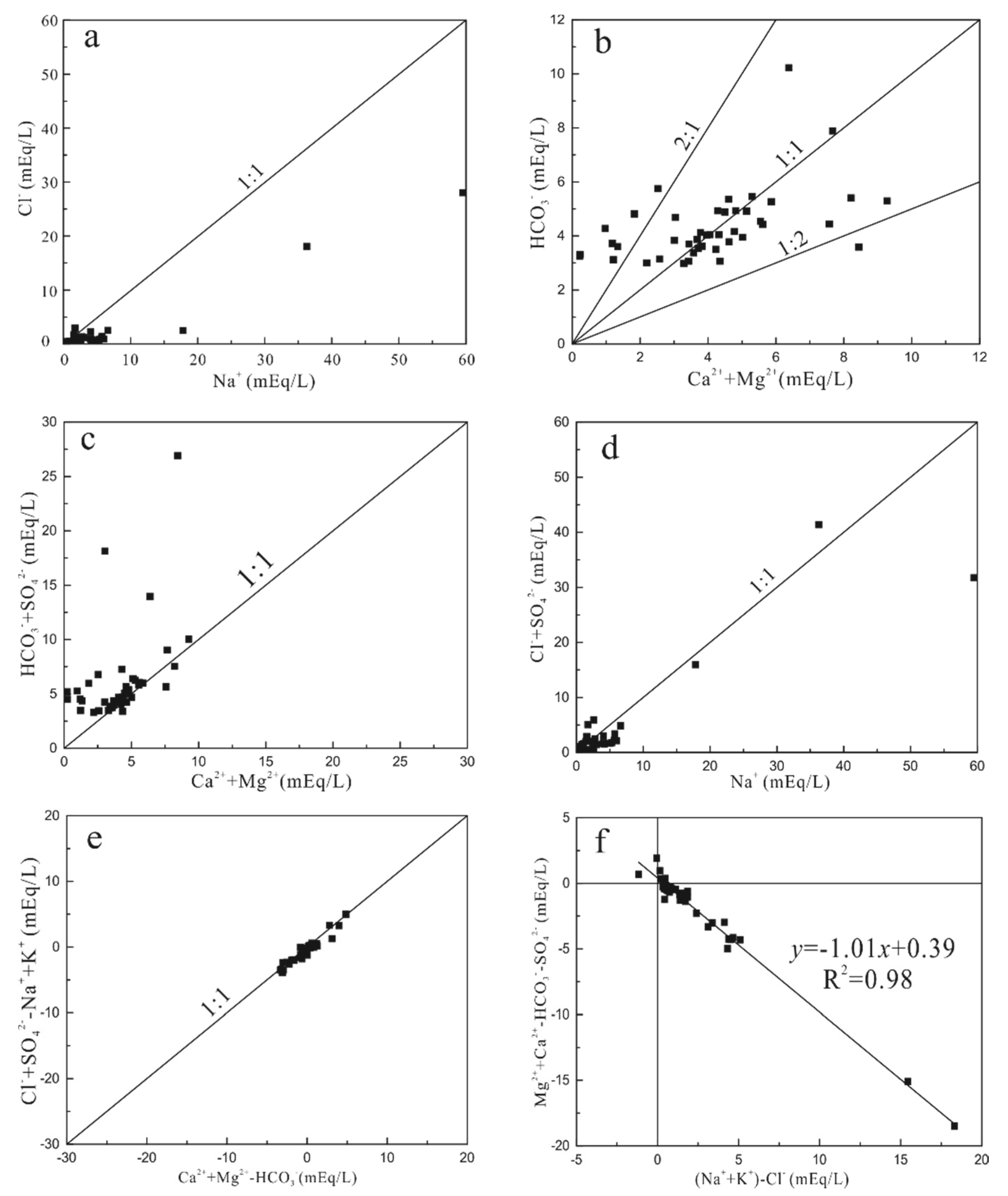
The Na+ and Cl− in meteoric water infiltrating into groundwater were nearly equal in concentration. The groundwater samples collected from most sampling sites were near the 1:1 line in Figure 3a, suggesting that the groundwater originated primarily from meteoric water. In addition, halite dissolution releases Na+ and Cl− in equal concentration to the groundwater. Groundwater samples collected from some sampling sites were below the 1:1 line, indicating that the hydrolysis of other Na-containing minerals had led to an excess of Na+. The weathering and dissolution of carbonate minerals (e.g., calcite and dolomite) is the principal source of Ca2+ and Mg2+ in groundwater. The ratio of the combined milligram equivalent concentration of Ca2+ and Mg2+ to the milligram equivalent concentration of HCO3− was found to be 1.
The groundwater samples collected from most of the sampling sites were near the 1:1 line of Figure 3b, while samples retrieved from some sampling sites were near the 1:2 or 2:1 line. That the combined concentration of Ca2+ and Mg2+ was higher than the concentration of HCO3− may be attributed to the dependence of the weathering and dissolution of carbonate minerals or Ca and Mg feldspars on weak acids instead of strong acids or the presence of other sources of Ca2+ and Mg2+ (e.g., gypsum). That the combined concentration of Ca2+ and Mg2+ was lower than the concentration of HCO3− may be attributed to the increase in the concentration of HCO3− caused by silicate dissolution or the decrease in the combined concentration of Ca2+ and Mg2+ resulting from cation exchange.
The groundwater samples collected from most of the sampling sites were near the 1:1 line of Figure 3c, though those from some sampling sites were above the 1:1 line, suggesting the dissolution of other SO42−-containing minerals in the groundwater in addition to gypsum. Further, the groundwater samples collected from all the sampling sites were near the 1:1 line in Figure 3d, except for one outlier sample, indicating that mirabilite dissolution was the source of the excess of Na+ in the groundwater at some sampling sites. Under normal circumstances, the concentration of Cl− is stable in the groundwater environment, and Cl− does not undergo chemical or physical reactions with other ions or minerals. Groundwater samples collected from some sampling sites were above the 1:1 line, indicating the dissolution of other sulfates. Figure 3e mainly explains the linear relationship between the combined concentration of Ca2+ and Mg2+ originating from sources other than the dissolution of carbonates and feldspars and the concentration of SO42− originating from sources other than mirabilite dissolution. The groundwater samples were near this 1:1 line, suggesting gypsum dissolution in the groundwater.
Figure 3f reflects whether cation exchange, specifically between Na+ and Ca2+, occurred in the groundwater. A slope near −1 indicates the occurrence of cation exchange at a groundwater sampling site. As shown in Figure 3f, the slope of the fitted curve corresponding to each groundwater sampling site was −1.01, suggesting an exchange between Na+ and Ca2+ during the groundwater runoff process.
4.2. Formation of the Hydrochemical Composition of the Groundwater
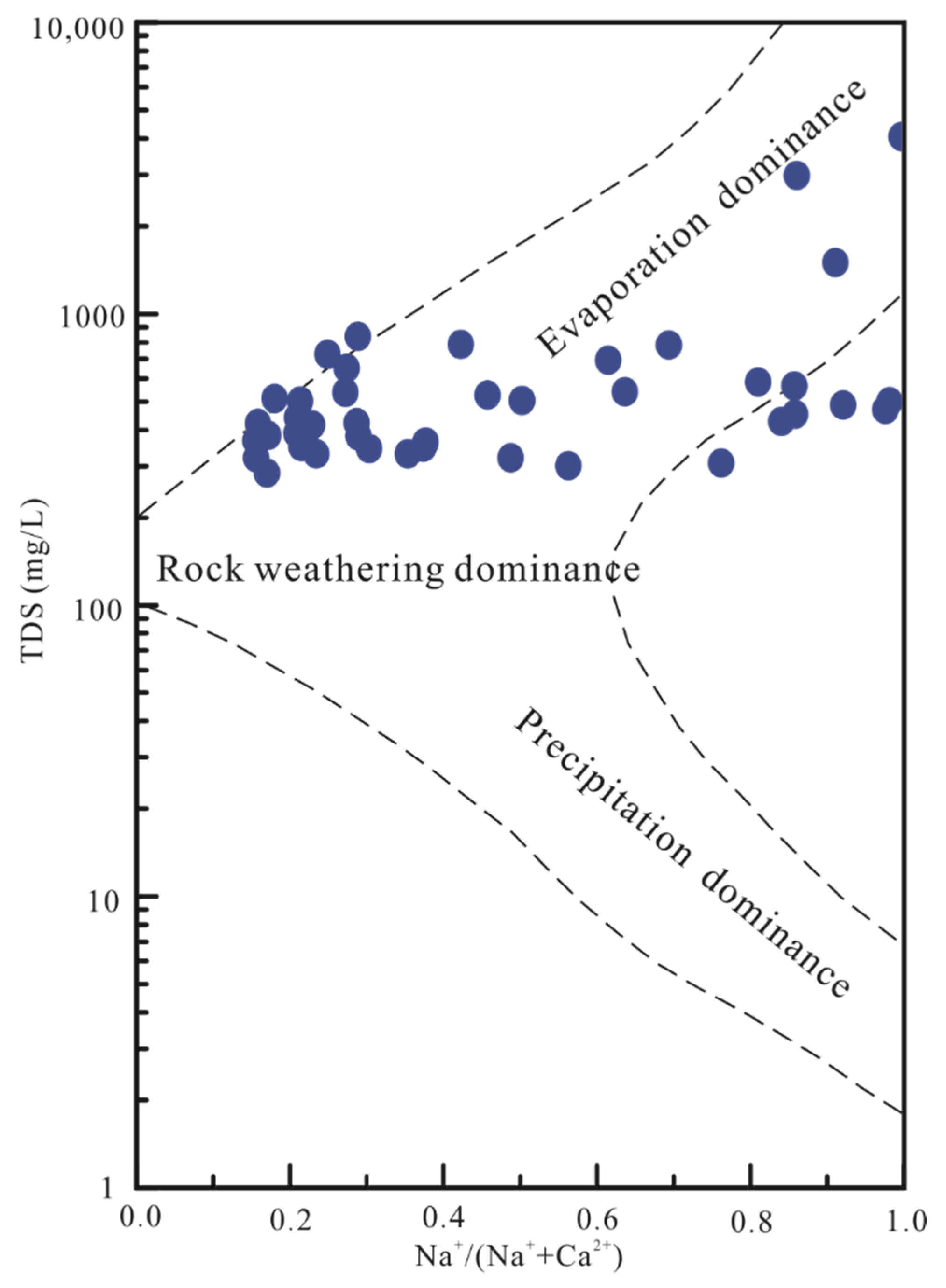
As seen in Figure 4, groundwater samples collected from most sampling sites fall in the water–rock interaction region on the Gibbs diagrams (TDS vs. Na+/(Na+ + Ca2+)), suggesting that the major constituents of the groundwater in the study area originate primarily from water–rock interactions that occur over a long time after the groundwater is recharged by infiltrated precipitation. Sampling site D69 was located in the upper reaches of the Zhasake River and at the northern boundary of the study area, where the groundwater was shallow. The concentration of total dissolved solids (TDS) at site D69 was 1499 mg/L. Sampling site D81 was located in the upper reaches of the Mudushili River and the heavily eroded northern part of the study area. The intense water–rock interactions and evaporation-induced concentration process in the piedmont recharge zone led to a high concentration of TDS (2985 mg/L, as found in this study) at site D81. The hydrochemical composition of the groundwater at most sampling sites was controlled by water–rock interactions. The ratio of the concentration of Na+ to the combined concentration of Na+ and Ca2+ (Na+/(Na+ + Ca2+)) was above 0.5 at most sampling sites, suggesting an exchange between Na+ and Ca2+ in the groundwater runoff [29,30].
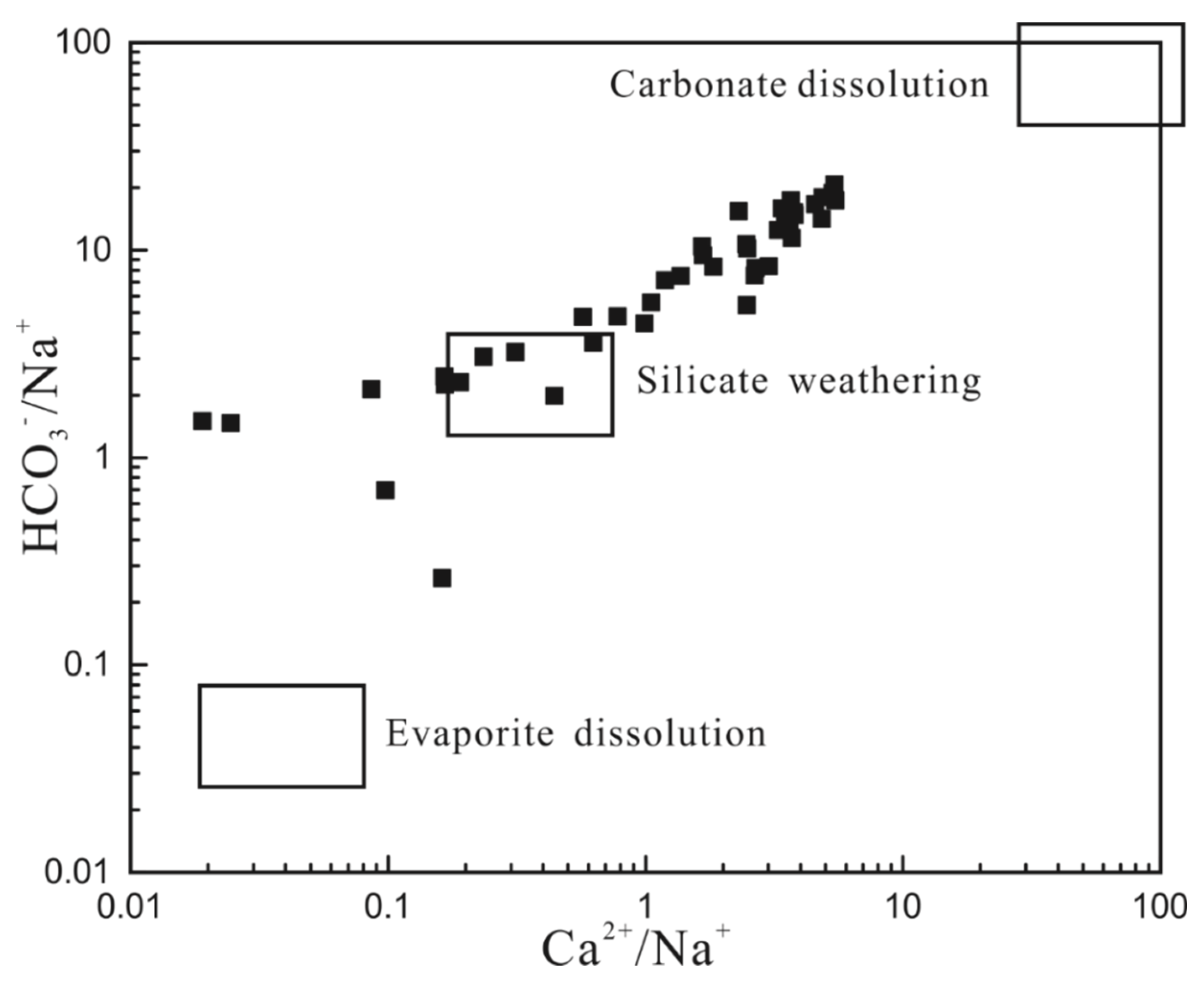
Gaillardet et al. [31] proposed using a Na-normalized molar ratio to reflect different hydrochemical reactions under non-mixed conditions. Compared to the Gibbs diagram, which can only indicate whether water–rock interactions are the dominant mechanism overall, this metric can identify particular water–rock interactions. The Gaillardet diagram consists of three regions that correspond to three respective hydrochemical processes: carbonate dissolution, silicate weathering, and evaporite dissolution. If a groundwater sample falls in a certain region of the graph, it means that the hydrochemical process depicted by that region plays a dominant role at the site where the sample was collected. If a groundwater sample falls between two regions, it suggests the coexistence of different hydrochemical processes at the site. As seen in Figure 5, groundwater samples collected from most sampling sites in the study area fell between the silicate weathering and carbonate dissolution regions on the Gaillardet diagram, suggesting that the composition of the groundwater in the study area is controlled predominantly by silicate weathering and carbonate dissolution. Due to their high concentrations of TDS, groundwater samples collected from some sampling sites (i.e., D63, D69, and D81) fell near the evaporite dissolution region.
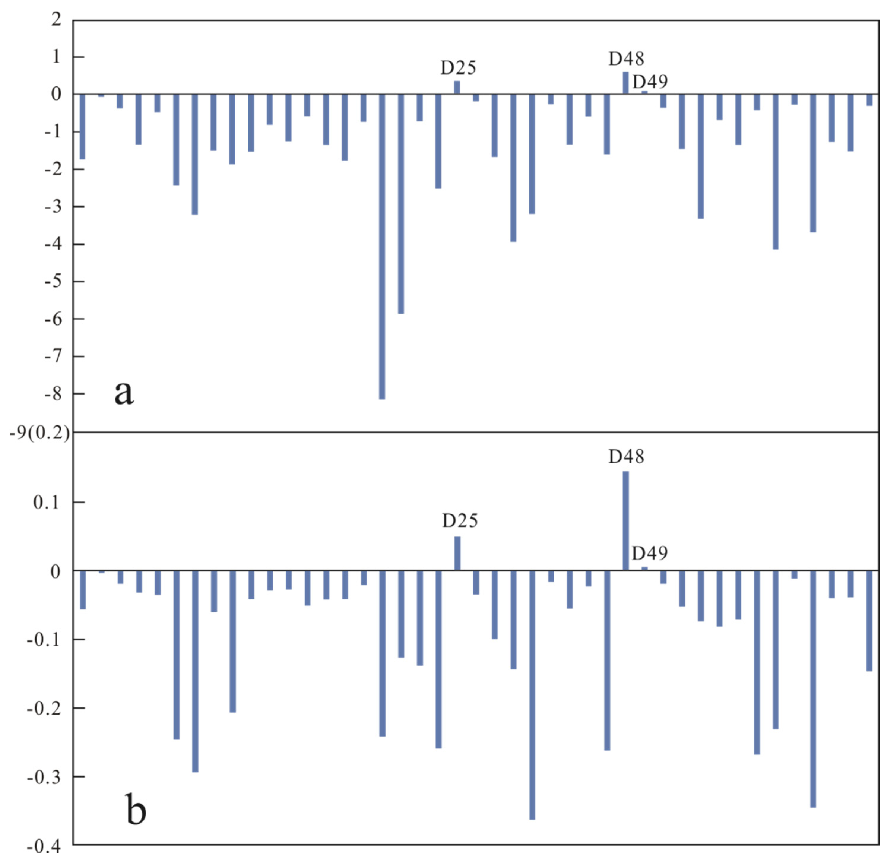
Cation exchange is a process in which particles adsorb some cations from the groundwater and simultaneously release some of the previously adsorbed cations back into the groundwater under certain conditions. The CAIs (CAI 1 and CAI 2) introduced by Schoeller [32] (see Equations (2) and (3)) were used to further investigate the cation exchange in the groundwater in the study area:
If both CAI 1 and CAI 2 are positive, it means that there is an exchange between the Na+ and K+ in the groundwater and the Ca2+ and Mg2+ in the surrounding rock; otherwise, it suggests an exchange between the Ca2+ and Mg2+ in the groundwater and the Na+ and K+ in the surrounding rock. High absolute values of CAI 1 and CAI 2 indicate a high cation exchange tendency [10].
As seen in Figure 6, the CAI 1 and CAI 2 values for groundwater samples collected from most sampling sites were below 0, suggesting that the cation exchange in the groundwater environment in the study area was dominated by the exchange between the Ca2+ and Mg2+ in the groundwater and the Na+ and K+ in the surrounding rocks. This result also pinpoints the source of the excess Na+ in the groundwater. The CAI 1 and CAI 2 values for the samples collected at sites D25, D48, and D49 were positive, suggesting an opposite exchange.
4.3. Analysis of Mineral Dissolution
The chemical reactions between groundwater and its surrounding rocks can be used to elucidate the characteristics of their interactions and to reveal the pattern of evolution of the hydrochemical composition of the groundwater. The hydrogeochemical simulation software PHREEQC can be used to simulate the geochemical processes in a groundwater system. The hydrogeochemical code PHREEQC is employed to conduct the calculation of SI speciation by using the database of phreeqc.dat. It calculates the SI for a given mineral under different controlled conditions based on hydrochemical data (Appendix A, Table A1) for the groundwater to reflect the equilibrium state of the mineral. On this basis, the role of one or multiple reactive minerals in controlling the hydrochemical composition of the groundwater can be determined [3,19]. The SI for a mineral can be calculated using Equation (4) to determine whether it dissolves or precipitates in the groundwater:
where IAP is the ion activity product and K is the equilibrium constant. A positive SI indicates that the mineral is oversaturated in the groundwater, tends to precipitate from it, and maybe is nonreactive; a negative SI suggests that the mineral is unsaturated in the groundwater and will thus tend to dissolve. If the absolute value of the SI falls within 0–0.5, the mineral is considered to be in an equilibrium state. A high absolute value of the SI suggests significant dissolution or precipitation of the mineral [3].
Table 2 summarizes the calculated values of the SI for gypsum, calcite, dolomite, halite, and fluorite. The values of the SI for halite, gypsum, and fluorite were all negative, while the values of the SI for calcite and dolomite ranged from negative to positive. The values of the SI for evaporite halite ranged from −8.86 to −4.55, averaging −7.59, suggesting considerable halite dissolution in the groundwater of the study area, which explains its high concentrations of Na+ and Cl−. The values of the SI for gypsum and fluorite ranged from −3.14 to −0.74 and from −4.12 to −1.10, respectively, with averages of −2.25 and −2.29, indicating that these two minerals also actively dissolve in the groundwater and are the main sources of Ca2+. The underground water-bearing media in the study area are rich in halite, gypsum, and fluorite. These minerals are the major sources of ions in the groundwater. These conclusions are consistent with the results of the earlier hydrochemical analysis of the groundwater.
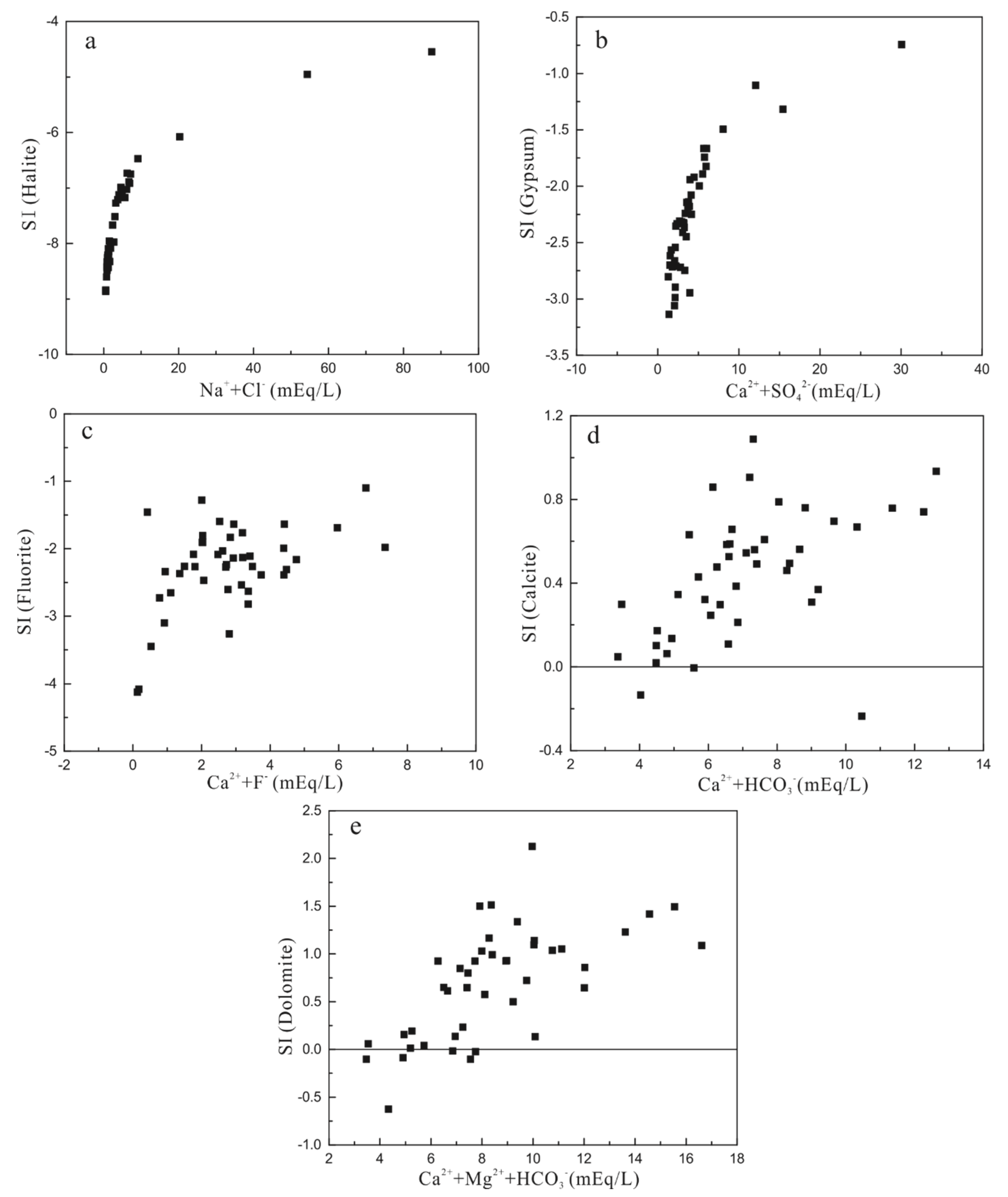
To further illustrate the relationships between the mineral dissolution or precipitation and the ions in the groundwater, the SI for each mineral and the concentrations of the corresponding ions were plotted in the same graph (Figure 7). As seen in Figure 7a, the SI for halite was positively correlated with the combined concentration of Na+ and Cl−, suggesting that halite dissolution is the primary source of Na+ and Cl− in the groundwater. As the combined concentration of Na+ and Cl− in the groundwater increased, the SI for halite increased first sharply and then more slowly after a certain total concentration of Na+ and Cl− was reached. A similar linear relationship was found between the SI for gypsum and the combined concentration of Ca2+ and SO42− (Figure 7b), indicating that gypsum actively dissolves in the groundwater and is the primary source of Ca2+ and SO42−. Fluorite dissolution can also provide Ca2+ to groundwater. Figure 7c reveals a positive correlation between the SI for fluorite and the combined concentration of Ca2+ and F−. The groundwater data points in Figure 7c are scattered, unlike those in Figure 7a,b, which are concentrated and exhibit strong linear relationships, indicating that compared to halite and gypsum, fluorite is the predominant source of ions in the groundwater.
The values of the SI for the carbonate minerals—calcite and dolomite—were mostly positive (Figure 7), suggesting that these minerals may exist in the water-bearing media and control the hydrochemical composition of the groundwater. As seen in Figure 7d, the SI for calcite in the groundwater at three sampling sites was negative and gradually increased with an increase in the total concentration of Ca2+ and HCO3−, indicating that most calcite in the groundwater exists in the form of precipitates or is reactive. The SI for dolomite in the groundwater at six sampling sites was negative (Figure 7e). The variation in dolomite with the change in the total concentration of the corresponding ions is similar to that of calcite with the total concentration of Ca2+ and HCO3−, suggesting that dolomite also precipitates in the groundwater. The carbonate minerals in the groundwater in the study area were nonreactive or precipitates. In addition, the groundwater environment had a low combined concentration of Ca2+ and Mg2+ and a high concentration of HCO3−. These findings are consistent with the earlier analysis of the hydrochemical characteristics of the groundwater and the formation of its hydrochemical composition. Silicate minerals are dissolved in the groundwater. Moreover, hydrogeological drilling data reveal that the sandstones in the Cretaceous Luohe and Huanhe formations contain feldspar minerals. The precipitation of calcite and dolomite decreases the combined concentration of Ca2+ and Mg2+ in the groundwater and yields a large amount of free CO2. Excessive CO2 dissolution in the groundwater promotes the dissolution of Na and K feldspars.
4.4. Hydrochemical Facies of Groundwater
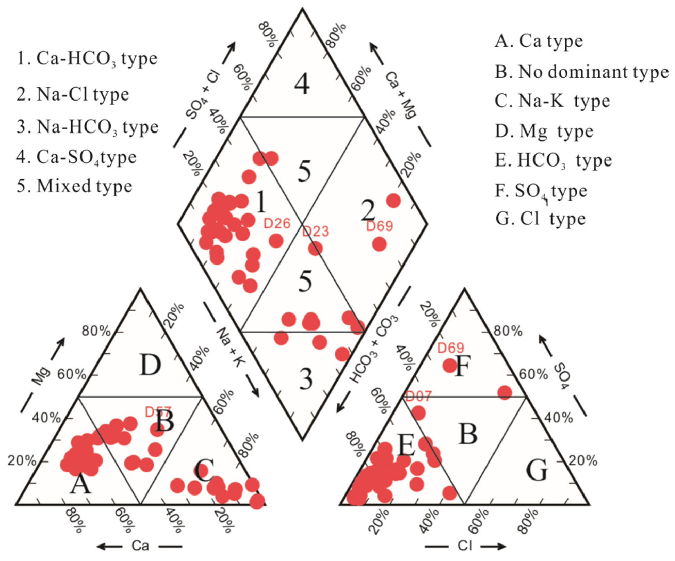
Groundwater samples collected from most sampling sites fell in region 1 on the Piper trilinear diagram in Figure 8, corresponding to an HCO3–Ca facies. The samples collected from sites D69 and D81 fell in region 2, corresponding to a Cl–Na facies, while those collected from sites D10, D21, and D39 fell in region 3, corresponding to an HCO3–Na facies. The other water samples fell in region 5, corresponding to mixed hydrochemical facies. Calculations performed based on an ion milligram equivalent percentage of over 25% revealed an HCO3–SO4–Ca facies at site D07, an HCO3–Cl–Na–Ca facies at site D23, an HCO3–SO4–Na facies at site D47, an HCO3–Cl–Na facies at site D63, and an HCO3–Na–Ca facies at sites D09, D13, D24, and D66. In addition, the anion and cation trilinear diagrams similarly showed that Ca, Na, and Ca–Na were the dominant cations and that HCO3 was the dominant anion.
The spatial variation of the hydrochemical facies of the groundwater was investigated based on the above hydrochemical facies analysis combined with the groundwater contour map. Groundwater flows from site D10, located on the shore of the Hongjiannao Lake, to Hongjiannao Lake and the nearby lake water sampling site D34. The hydrochemical facies of the groundwater transition from HCO3–Na at site D10 to Cl–Na at site D34. Analysis of the SI for the minerals at site D34 revealed a positive SI value for each of calcite and dolomite and a negative SI value for halite, suggesting that the HCO3− in the groundwater runoff combines with Ca and Mg to form precipitates and that Cl− replaces HCO3− and combines with Na+ to form a new hydrochemical facies. HCO3–Ca was the hydrochemical facies at both sampling sites D22 and D26, located in the recharge zone for the groundwater at site D23, which is of the HCO3–Cl–Na–Ca mixed facies. Analysis showed positive SI values for calcite and dolomite and negative SI values for halite at these three sampling sites, suggesting that halite actively dissolves in the groundwater runoff, releasing more Na+ and Cl−, which in turn leads to a transition in the hydrochemical facies to a mixed combination of HCO3–Ca and Cl–Na. The above analysis based on the SI values of minerals reveals a spatial variability in the hydrochemical facies of the groundwater in the study area.
4.5. SOM-Based Clustering
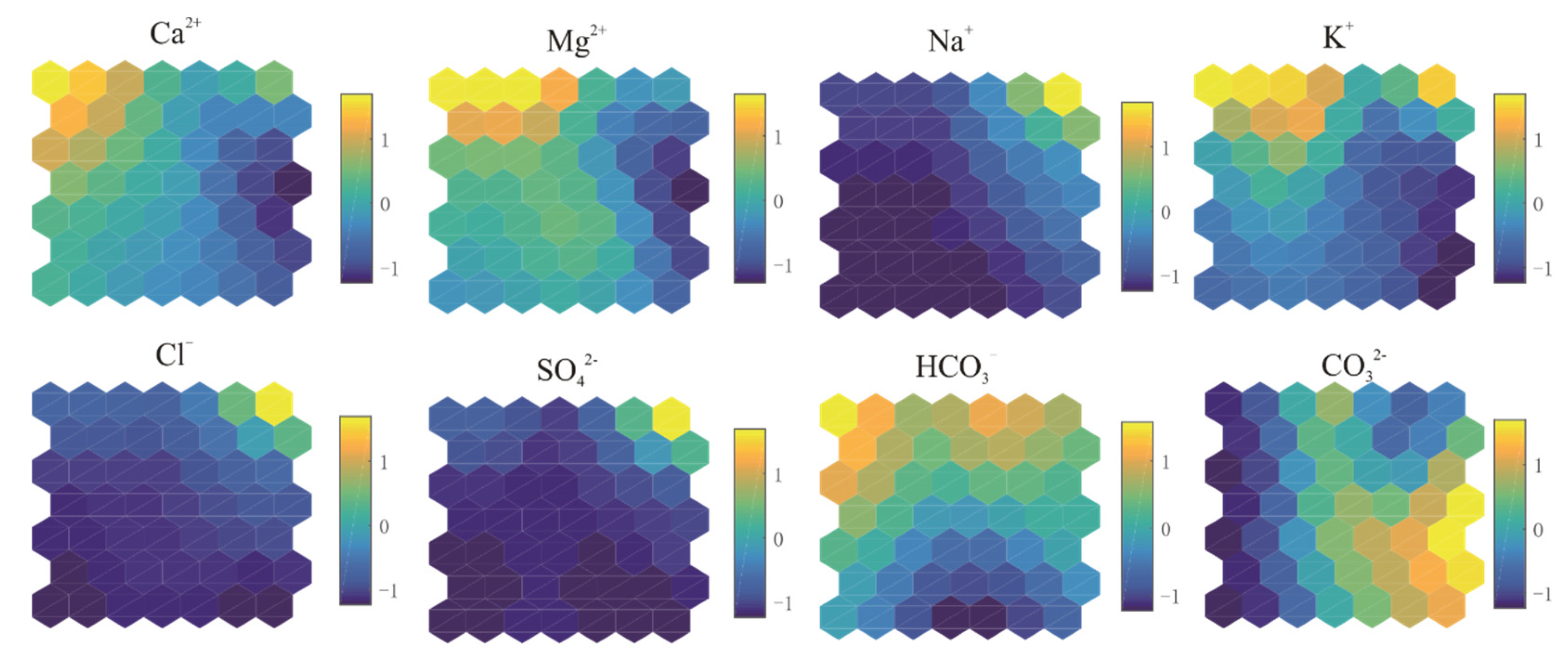
SOMs were trained on the hydrochemical data for the groundwater sampled in the rainy and dry seasons and were then used to normalize these data. SOMs for eight hydrochemical parameters were obtained (Figure 9). In each map, the color shade of each neuron represents the component value of the hydrochemical parameter of the groundwater at the sampling site. These maps visually display the distances between the corresponding neurons and the distribution of their color shades and elucidate the information and qualitative relationships between the hydrochemical parameters. In Figure 9, the SOMs for the concentrations of Ca2+, Mg2+, K+, and HCO3− display similar color gradients, suggesting strong correlations between the concentrations of these ions. The correlations between the concentrations of Ca2+, Mg2+, and HCO3− in the groundwater indicate that they may originate from the dissolution of calcite and dolomite. The correlation between the concentrations of K+ and HCO3− suggests the dissolution of K feldspars in the groundwater. On the other hand, the SOM for the concentration of CO32− exhibits a color gradient opposite to those of the SOMs for the concentrations of the other seven ions, indicating that the concentration of CO32− is negatively correlated with each of the other seven ion concentrations. The SOMs for the Na+, Cl−, and SO42− concentrations displayed similar color gradients, suggesting strong positive correlations between them. The positive correlation between the concentrations of Na+ and Cl− was primarily a result of halite dissolution in the groundwater, while the correlation between the Na+ and SO42− concentrations may be attributed to mirabilite dissolution. Ca2+ and SO42− originate from gypsum dissolution. The SOMs revealed a weak positive correlation between the concentrations of these two ions.
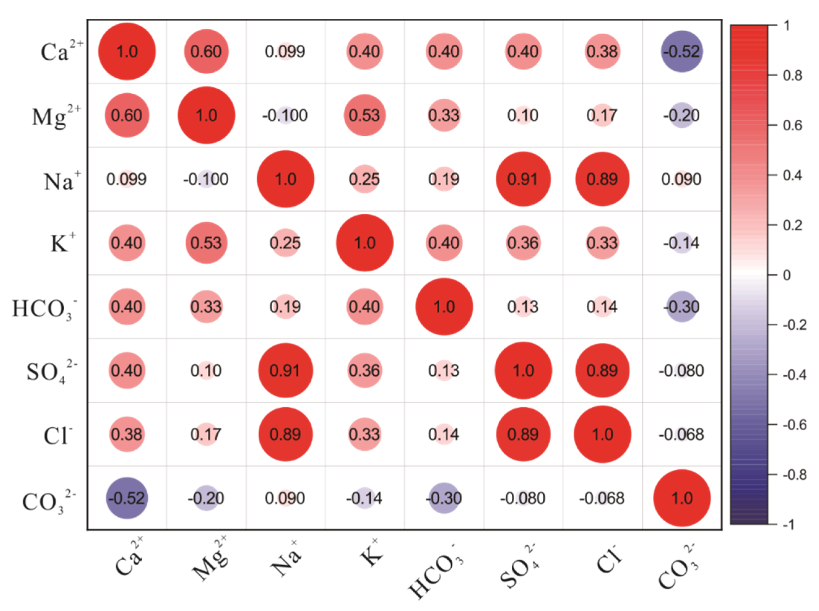
Meanwhile, the correlation heatmap was plotted using the hydrochemical data, as shown in Figure 10. The correlation heatmap of the same variable is shown by the largest and darkest solid circle. As the correlation decreases, the solid circles become smaller and lighter in color, so it can intuitively check the correlation between different variables. There was a strong positive correlation between the concentrations of any two of Ca2+, Mg2+, K+, HCO3−, Cl−, and SO42−. The concentration of CO32− was negatively correlated with that of each of the other ions besides HCO3−. The concentration of Na+ was most strongly positively correlated with the concentration of each of HCO3−, Cl−, and SO42−. The results of the correlation heatmap are basically consistent with those of the SOM-based analysis, suggesting that the SOMs can be used to represent the correlations between these parameters.
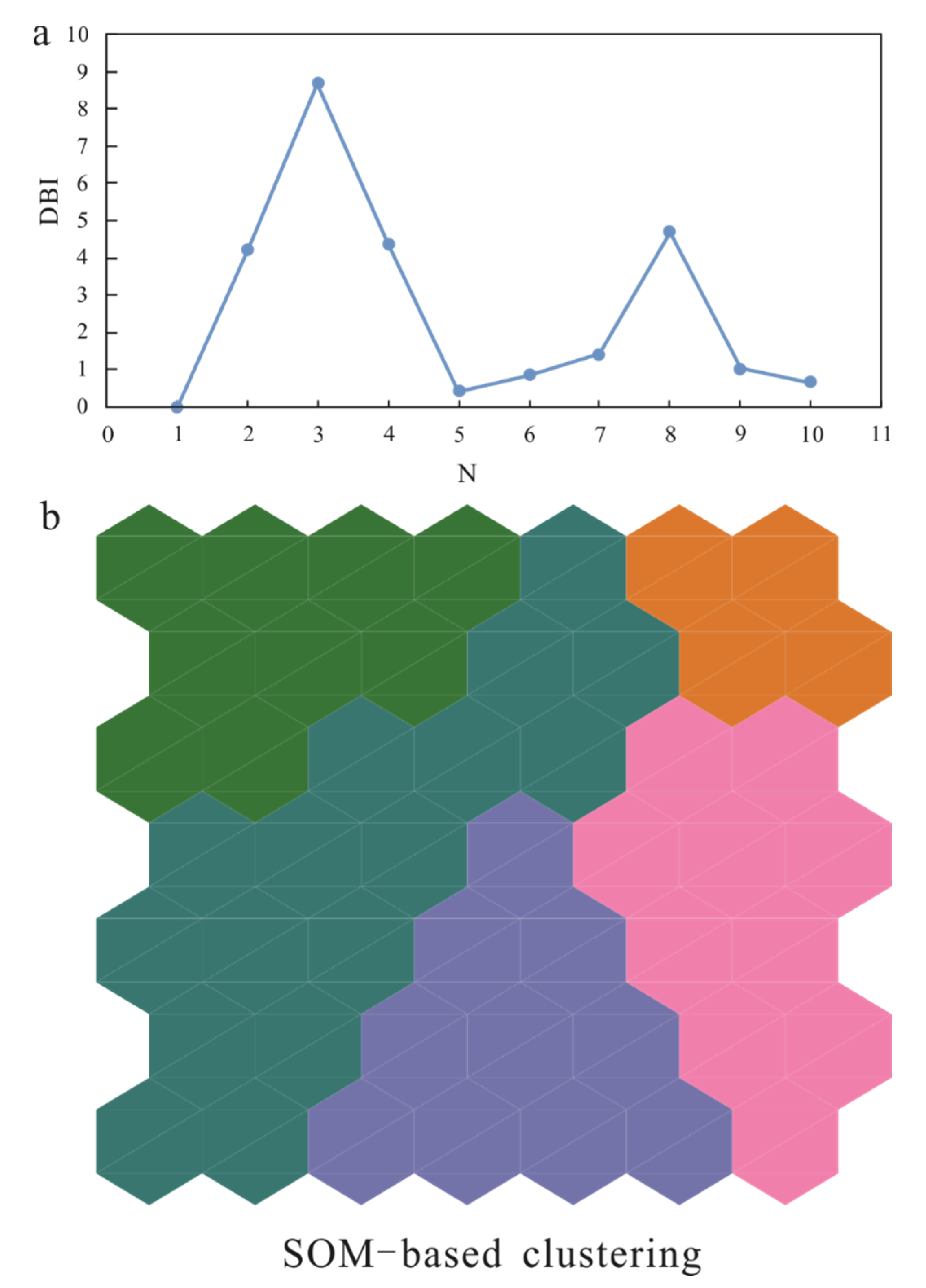
The trained SOM-normalized hydrochemical data for the groundwater in the study area in the rainy and dry seasons were used as the input matrix X in the calculation of the DBI. We set N equal to 10. Figure 11 shows the calculated values of the DBI. As seen in Figure 11a, the minimum DBI occurred at Nc = 5. Therefore, Nc was set to 5 for the cluster analysis in this study. Based on the optimal Nc, the groundwater samples collected during the rainy and dry seasons were clustered through SOM-based calculations. In Figure 11b, the five clusters are distinguished with different colors. The neurons covered with the same color represent one cluster. Each cluster contains groundwater samples with similar hydrogeochemical characteristics.
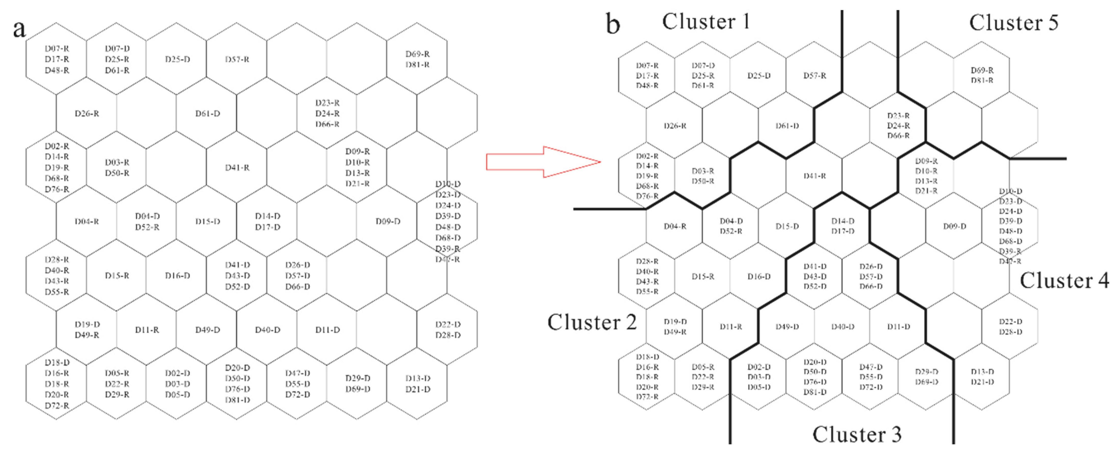
Figure 12 shows the SOMs for the groundwater samples collected from the study area during the rainy and dry seasons. This diagram was produced through repetitive iterations, self-organizing learning, and training based on the SOM algorithms to facilitate the visual output and cluster analysis. Groundwater samples with similar hydrogeochemical characteristics were assigned to the same SOM neuron (the suffixes R and D signify rainy- and dry-season samples, respectively). The temporal and spatial variability of the hydrochemical composition of the groundwater in the study area was further analyzed based on the distance between the neurons containing the samples collected during different seasons at each sampling site. Figure 12b gives a visual representation of the clustering of the groundwater samples collected from the study area during the rainy and dry seasons based on a combination of Figure 11b and Figure 12a. It shows that the groundwater samples were grouped into five clusters as well as which groundwater samples made up each cluster. Analysis based on the locations of the groundwater samples depicted in the SOMs in Figure 9 identified Ca2+, Mg2+, K+, and HCO3− as the dominant ions in the groundwater samples in cluster 1 and Na+, K+, Cl−, and SO42− as the dominant ions in the groundwater samples in cluster 5.
4.6. Analysis of Clustered Hydrochemical Characteristics
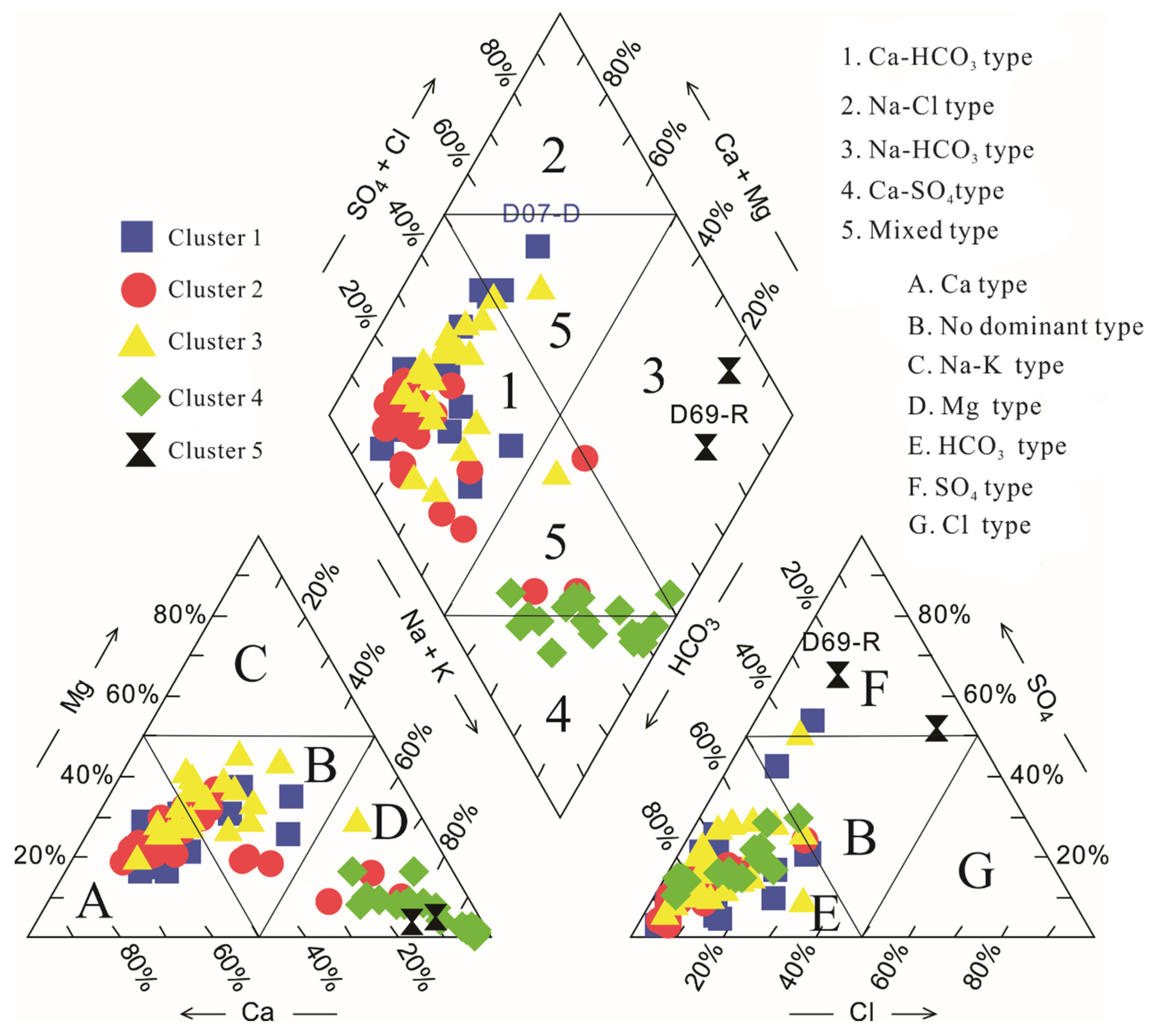
To comprehensively evaluate the hydrochemical clustering of the groundwater in the study area in the rainy and dry seasons, a Piper trilinear diagram was produced based on the hydrochemical data for each SOM-yielded cluster of groundwater samples (Figure 13). The groundwater samples in cluster 1 mostly fell in region 1, with their anions falling in region E and their cations falling in regions A and B, suggesting HCO3–Ca as their hydrochemical facies. This finding is consistent with the earlier analysis of the groundwater samples in this cluster: Ca2+, Mg2+, and HCO3− were identified as their dominant ions. Similarly, HCO3–Ca was the hydrochemical facies of the groundwater samples in cluster 2. The Piper diagram reveals the presence of weak cations in the groundwater samples in cluster 2, which is consistent with the conclusion drawn from the color gradient in the SOM for the concentration of Ca2+ in Figure 9. The groundwater samples in cluster 3 fell in the same region as those in cluster 1, suggesting HCO3–Ca as their hydrochemical facies. The groundwater samples in cluster 4 mostly fell on the border between regions 4 and 5, their cations falling in region D and their anions falling in region E, suggesting HCO3–Na as their hydrochemical facies, which is consistent with the SOMs for the concentration of Na+ and HCO3−. Cluster 5 contained only two groundwater samples. They fell in region 3, their cations falling in region D and their anions falling in region F, indicating Cl–Na as their hydrochemical facies. Overall, HCO3–Ca type and HCO3–Na type were the dominant hydrochemical facies of the groundwater in the study area during the rainy and dry seasons.
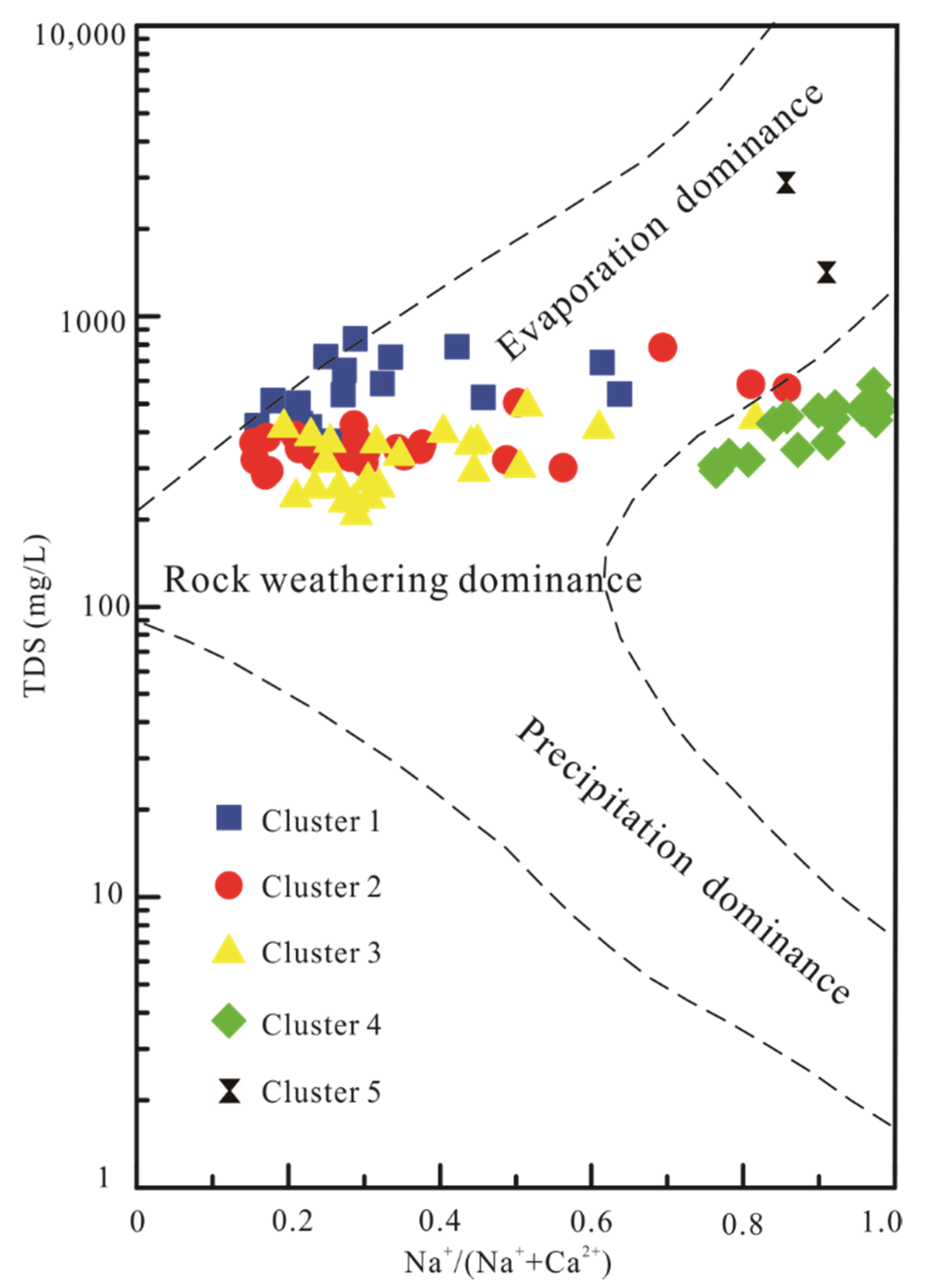
Figure 14 shows a Gibbs diagram for the clusters obtained based on the SOMs (TDS vs. Na+/(Na+ + Ca2+)). The groundwater samples in clusters 1, 2, 3, and 4 mostly fell in the region corresponding to water–rock interaction dominance. The groundwater samples in cluster 1 fell on the edge of the evaporation-induced concentration region, suggesting that the groundwater at the sites where these samples were collected is also affected by the evaporation-induced concentration process. Of the groundwater samples in clusters 1, 2, and 3, those in cluster 1 had the highest average concentration of TDS, followed by those in clusters 2 and 3. Based on the SOMs (in the upper-left corner of Figure 9), the high concentration of TDS in the groundwater samples in cluster 1 can be attributed to their high concentrations of Ca2+, Mg2+, and HCO3−. With a Na+/(Na+ + Ca2+) ratio of greater than 0.7, the groundwater samples in cluster 4 fell outside the region encircled by the dotted lines, suggesting intense cation exchange in the groundwater environment where these samples were collected. With a high Na+/(Na+ + Ca2+) ratio, the groundwater samples in cluster 5 fell in the evaporation-induced concentration region, suggesting that the hydrochemical composition of the groundwater where these two samples were collected is dually affected by the evaporation-induced concentration process and cation exchange. Overall, the hydrochemical composition of the groundwater in the study area during the rainy and dry seasons is primarily controlled by water–rock interactions.
4.7. Seasonal Variability
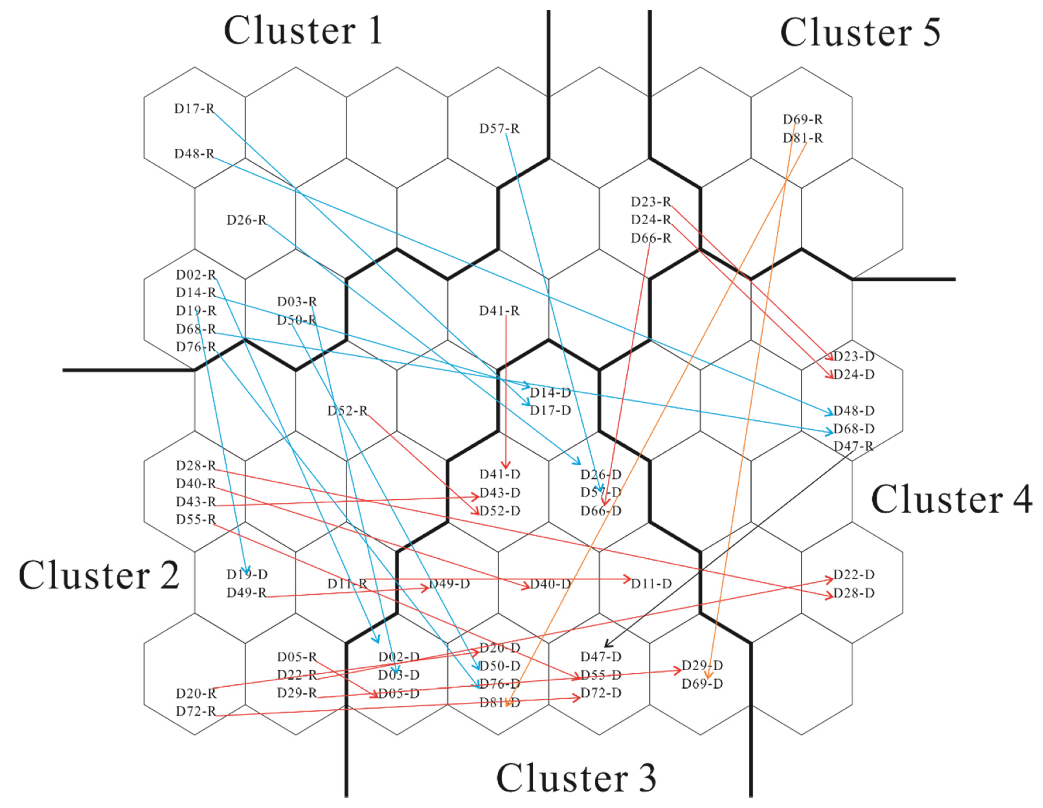
The seasonal variability of the groundwater in the study area during the rainy and dry seasons was further analyzed. Figure 15 visually depicts the changes in the clustering of the sampling sites corresponding to the change from the rainy season to the dry season, which was determined based on the topological distances between the SOM neurons in combination with the cluster analysis. Changes can be observed in the clustering of 30 sampling sites. The blue arrows show the changes in the clustering of the sampling sites in cluster 1 (a total of 11 sampling sites) corresponding to a change from the rainy season to the dry season. A change from cluster 1 to cluster 2 was observed in the assignment of one sampling site (D19), while a change from cluster 1 to cluster 3 was observed in the assignment of eight sampling sites. Based on the above analysis of the hydrochemical facies of the groundwater and the formation of its hydrochemical composition, there was weak seasonal variability in the hydrochemical characteristics of the groundwater at these nine sampling sites. A change from cluster 1 to cluster 4 was observed in the assignment of two sampling sites, corresponding to a change in the hydrochemical facies from HCO3–Ca to HCO3–Na, suggesting that the formation of the hydrochemical composition of the groundwater at these sites is accompanied by an intense cation-exchange process and that there is a strong seasonal variability in the hydrochemical characteristics of the groundwater at these two sites.
The red arrows in Figure 15 show the changes in the clustering of the sampling sites in cluster 2 (a total of 11 sampling sites) corresponding to a change from the rainy season to the dry season. A change from cluster 2 to cluster 3 was observed in the assignment of 12 sampling sites, suggesting no significant changes in the hydrochemical characteristics of the groundwater at these sites. A change from cluster 2 to cluster 4 was observed in the assignment of four sampling sites, corresponding to a change in the hydrochemical facies from HCO3–Ca type to HCO3–Na type, which suggests that the formation of the hydrochemical composition of the groundwater at these sites is controlled by cation exchange. A change from cluster 5 to cluster 3 was found in the assignment of two sampling sites, corresponding to a change in the hydrochemical facies from Cl–Na to HCO3–Ca, which indicates that the formation of the hydrochemical composition of the groundwater at these sites changed from an evaporation-induced concentration-dominated mechanism to a water–rock-interaction-dominated mechanism and that there is a strong seasonal variability in the hydrochemical characteristics of the groundwater at these sites. A change from cluster 4 to cluster 3 was observed in the assignment of one sampling site, corresponding to a change in the hydrochemical facies from HCO3–Na to HCO3–Ca, which suggests a weak cation-exchange process and a notable seasonal variability in the hydrochemical characteristics of the groundwater at this site. Overall, the SOM-based seasonal variability diagram reveals changes in the clustering of 30 sampling sites and a notable seasonal variability in the hydrochemical characteristics of the groundwater at nine sampling sites. The hydrochemical characteristics of the groundwater in the study area exhibited no significant seasonal variability.
5. Conclusions
- (1)
- The formation of the hydrochemical composition of the groundwater in the study area during the rainy and dry seasons is controlled by water–rock interactions and cation exchange. Three hydrochemical facies, HCO3–Ca type, HCO3–Na type, and Cl–Na type, dominate the groundwater in the study area, whose composition is controlled primarily by silicate weathering and carbonate dissolution. Halite, gypsum, and fluorite are the dominant sources of ions in the groundwater in the study area. Dolomite and calcite exist mostly in the form of precipitates or reactive minerals in the groundwater of the study area, in which a small amount of feldspar is dissolved.
- (2)
- SOMs were used to cluster the data of the hydrochemical parameters of the groundwater in the rainy and wet seasons. Based on the QE, the TE, and the empirical equation, the number of neurons was optimized to 7 × 7. The results derived from the neuron matrices are consistent with those of the Pearson correlation analysis. The number of clusters was optimized through DBI minimization. The groundwater samples collected from the study area during the rainy and dry seasons are grouped into five clusters, with Ca2+, Mg2+, K+, and HCO3− identified as the dominant ions in cluster 1 and Na+, K+, Cl−, and SO42− identified as the dominant ions in cluster 5.
- (3)
- HCO3–Ca type is the hydrochemical facies of the groundwater samples in clusters 1, 2, and 3, while HCO3–Na type and Cl–Na type are the hydrochemical facies of the groundwater samples in clusters 4 and 5, respectively. Cation exchange is the dominant factor controlling the formation of the hydrochemical composition of the groundwater at the sites where the groundwater samples in cluster 4 were collected, compared to water–rock interactions for the sites where the groundwater samples in other clusters were collected. The clustering of 30 sampling sites changes with the transition from the rainy season to the dry season. Of these sites, significant seasonal variability was observed in the hydrochemical characteristics of the groundwater at nine sites. Overall, there was no significant seasonal variability in the hydrochemical characteristics of the groundwater in the study area.
Author Contributions
Conceptualization, C.W. and X.W.; data curation, C.W., X.W. and C.L.; formal analysis, C.W., Q.S., X.H. and L.Y.; funding acquisition, C.W., X.W. and Q.S.; investigation, C.W. and X.W.; methodology, C.W. and X.W.; project administration, C.W. and X.W.; resources, C.W.; software, C.W. and T.Q.; supervision, C.W. and X.W.; validation, C.W.; visualization, C.W. and X.W.; writing—original draft, C.W.; writing—review & editing, C.W. and X.W. All authors have read and agreed to the published version of the manuscript.
Funding
This research was supported by the National Key R&D Program of China (No.2017YF100408), Applied Technology Research and Development Program of Heilongjiang Province (GA19C005), National Natural Science Foundation of China (41572227).
Institutional Review Board Statement
Not applicable.
Informed Consent Statement
Not applicable.
Data Availability Statement
Not applicable.
Conflicts of Interest
The authors declare no conflict of interest.
Appendix A

Table A1.
Statistical summary for the hydrochemical parameters of groundwater samples (sample locations shown in Figure 1; D02-R represents the sample that was taken during the rainy season; and D02-D represents the sample that was taken during the dry season; unit: mg/L).
Table A1.
Statistical summary for the hydrochemical parameters of groundwater samples (sample locations shown in Figure 1; D02-R represents the sample that was taken during the rainy season; and D02-D represents the sample that was taken during the dry season; unit: mg/L).
| Sample | Ca2+ | Mg2+ | Na+ | K+ | HCO3− | SO42− | Cl− | CO32− |
|---|---|---|---|---|---|---|---|---|
| D02-R | 42.80 | 15.60 | 33.80 | 1.10 | 93.50 | 94.80 | 16.70 | 0.00 |
| D03-R | 35.00 | 16.80 | 15.40 | 2.04 | 129.00 | 48.40 | 15.70 | 0.00 |
| D04-R | 44.20 | 16.50 | 23.10 | 2.50 | 203.00 | 40.50 | 20.70 | 0.00 |
| D05-R | 37.40 | 10.70 | 9.94 | 1.37 | 142.00 | 29.30 | 5.10 | 0.00 |
| D07-R | 116.00 | 27.40 | 58.40 | 1.70 | 204.00 | 255.00 | 43.30 | 0.00 |
| D09-R | 10.70 | 2.89 | 121.00 | 1.01 | 197.00 | 48.50 | 35.20 | 6.85 |
| D10-R | 13.50 | 6.67 | 120.00 | 1.15 | 244.00 | 42.20 | 27.60 | 14.10 |
| D11-R | 30.90 | 14.10 | 31.60 | 1.11 | 156.00 | 27.80 | 9.11 | 8.98 |
| D13-R | 16.80 | 7.62 | 54.40 | 0.56 | 177.00 | 22.60 | 4.67 | 8.98 |
| D14-R | 76.70 | 13.30 | 18.50 | 0.59 | 220.00 | 51.90 | 8.30 | 10.00 |
| D15-R | 46.60 | 16.00 | 18.30 | 2.09 | 192.00 | 20.20 | 8.17 | 8.08 |
| D16-R | 50.10 | 10.70 | 10.60 | 1.20 | 188.00 | 21.20 | 5.28 | 5.39 |
| D17-R | 62.20 | 16.20 | 18.60 | 1.06 | 209.00 | 45.40 | 10.90 | 8.78 |
| D18-R | 50.90 | 12.30 | 16.90 | 0.85 | 205.00 | 23.20 | 6.97 | 0.00 |
| D19-R | 45.30 | 13.60 | 19.40 | 1.09 | 201.00 | 23.70 | 8.43 | 0.00 |
| D20-R | 41.70 | 11.00 | 12.80 | 0.90 | 109.00 | 36.30 | 7.94 | 4.64 |
| D21-R | 16.20 | 4.65 | 67.50 | 0.41 | 181.00 | 24.80 | 7.14 | 7.46 |
| D22-R | 18.70 | 5.14 | 66.80 | 0.64 | 182.00 | 25.20 | 4.10 | 10.70 |
| D23-R | 5.38 | 1.30 | 139.00 | 0.61 | 221.00 | 54.20 | 37.30 | 11.00 |
| D24-R | 5.12 | 0.05 | 177.00 | 0.67 | 237.00 | 94.50 | 37.90 | 13.30 |
| D25-R | 79.00 | 35.30 | 37.80 | 2.51 | 189.00 | 60.80 | 61.20 | 10.30 |
| D26-R | 19.10 | 22.30 | 84.50 | 1.08 | 181.00 | 20.50 | 59.60 | 12.20 |
| D28-R | 11.70 | 4.72 | 79.50 | 0.40 | 198.00 | 28.00 | 5.67 | 11.60 |
| D29-R | 36.60 | 11.60 | 17.20 | 0.66 | 132.00 | 21.00 | 7.68 | 9.03 |
| D39-R | 6.22 | 1.88 | 137.00 | 0.96 | 213.00 | 58.90 | 31.80 | 12.30 |
| D40-R | 25.70 | 21.90 | 21.00 | 1.16 | 144.00 | 13.10 | 13.60 | 7.65 |
| D41-R | 42.50 | 25.30 | 28.90 | 0.88 | 155.00 | 41.50 | 24.00 | 7.73 |
| D43-R | 39.20 | 21.00 | 13.10 | 1.14 | 179.00 | 16.50 | 11.90 | 6.37 |
| D47-R | 33.80 | 10.50 | 12.80 | 0.77 | 114.00 | 24.80 | 5.71 | 5.51 |
| D48-R | 3.30 | 1.66 | 127.00 | 0.27 | 202.00 | 42.80 | 43.80 | 9.91 |
| D49-R | 54.90 | 17.70 | 25.40 | 1.43 | 155.00 | 61.00 | 45.00 | 4.84 |
| D50-R | 37.00 | 13.90 | 13.50 | 1.29 | 93.00 | 15.70 | 15.60 | 5.09 |
| D52-R | 43.50 | 20.10 | 23.10 | 2.41 | 146.00 | 57.30 | 27.00 | 9.76 |
| D55-R | 44.70 | 12.10 | 15.30 | 1.32 | 148.00 | 17.40 | 9.48 | 6.96 |
| D57-R | 30.10 | 17.70 | 24.20 | 0.75 | 172.00 | 7.90 | 5.36 | 10.30 |
| D61-R | 45.70 | 14.80 | 15.90 | 5.75 | 180.00 | 9.51 | 20.90 | 12.40 |
| D66-R | 25.30 | 27.10 | 39.50 | 0.83 | 158.00 | 23.90 | 22.90 | 10.60 |
| D68-R | 11.30 | 13.40 | 117.00 | 0.72 | 255.00 | 43.70 | 23.00 | 18.20 |
| D69-R | 19.90 | 11.30 | 21.10 | 0.78 | 122.00 | 8.57 | 4.57 | 8.08 |
| D72-R | 31.80 | 14.70 | 13.00 | 1.18 | 122.00 | 37.70 | 6.24 | 7.91 |
| D76-R | 32.90 | 11.40 | 14.60 | 1.61 | 114.00 | 39.10 | 8.30 | 5.57 |
| D81-R | 30.30 | 15.80 | 12.20 | 0.43 | 110.00 | 12.90 | 12.80 | 4.71 |
| D02-D | 88.00 | 14.80 | 32.90 | 1.31 | 270.00 | 78.90 | 12.50 | 0.00 |
| D03-D | 68.10 | 19.70 | 12.80 | 1.99 | 241.00 | 35.20 | 13.80 | 0.00 |
| D04-D | 63.30 | 14.10 | 16.70 | 2.42 | 247.00 | 31.30 | 13.90 | 0.00 |
| D05-D | 49.30 | 10.10 | 10.10 | 1.55 | 182.00 | 23.50 | 4.98 | 0.00 |
| D07-D | 147.00 | 23.50 | 59.60 | 1.91 | 323.00 | 228.00 | 41.70 | 0.00 |
| D09-D | 18.20 | 5.25 | 95.50 | 0.78 | 220.00 | 36.00 | 28.10 | 0.00 |
| D10-D | 10.50 | 5.45 | 122.00 | 0.72 | 261.00 | 47.10 | 29.10 | 0.00 |
| D11-D | 41.20 | 16.70 | 22.50 | 1.40 | 187.00 | 30.20 | 9.56 | 0.00 |
| D13-D | 15.30 | 5.09 | 92.30 | 0.68 | 227.00 | 38.00 | 32.40 | 0.00 |
| D14-D | 89.50 | 13.10 | 24.20 | 0.76 | 277.00 | 62.70 | 9.85 | 0.00 |
| D15-D | 35.00 | 15.40 | 15.20 | 1.97 | 234.00 | 19.90 | 9.49 | 0.00 |
| D16-D | 56.20 | 11.00 | 10.40 | 1.24 | 216.00 | 20.50 | 5.16 | 0.00 |
| D17-D | 87.70 | 40.00 | 64.20 | 9.73 | 481.00 | 55.40 | 46.60 | 0.00 |
| D18-D | 54.00 | 10.70 | 16.50 | 0.96 | 206.00 | 18.00 | 7.43 | 0.00 |
| D19-D | 74.70 | 13.20 | 19.80 | 1.12 | 301.00 | 21.20 | 7.56 | 0.00 |
| D20-D | 67.20 | 10.70 | 12.30 | 0.93 | 214.00 | 26.30 | 7.62 | 0.00 |
| D21-D | 18.40 | 3.61 | 59.00 | 0.48 | 190.00 | 18.00 | 6.50 | 0.00 |
| D22-D | 36.00 | 9.47 | 34.30 | 0.57 | 192.00 | 14.30 | 5.08 | 0.00 |
| D23-D | 67.10 | 11.40 | 152.00 | 0.95 | 301.00 | 112.00 | 89.10 | 0.00 |
| D24-D | 21.80 | 9.04 | 131.00 | 1.04 | 294.00 | 55.50 | 37.60 | 0.00 |
| D25-D | 95.20 | 34.30 | 35.90 | 2.42 | 271.00 | 58.40 | 59.40 | 0.00 |
| D26-D | 58.30 | 29.00 | 92.90 | 1.10 | 333.00 | 38.20 | 79.10 | 0.00 |
| D28-D | 55.40 | 15.70 | 55.90 | 0.59 | 247.00 | 30.60 | 21.10 | 0.00 |
| D29-D | 29.80 | 8.63 | 38.30 | 0.61 | 183.00 | 14.60 | 7.88 | 0.00 |
| D39-D | 3.37 | 0.72 | 138.00 | 0.75 | 202.00 | 58.10 | 33.10 | 14.60 |
| D40-D | 56.40 | 21.90 | 22.70 | 0.84 | 231.00 | 22.00 | 18.60 | 0.00 |
| D41-D | 40.10 | 21.60 | 24.20 | 1.33 | 252.00 | 6.26 | 10.90 | 6.29 |
| D43-D | 52.00 | 16.60 | 14.20 | 1.39 | 246.00 | 9.42 | 9.79 | 0.00 |
| D47-D | 2.51 | 1.18 | 132.00 | 0.38 | 198.00 | 93.80 | 50.80 | 11.00 |
| D48-D | 119.00 | 27.60 | 39.50 | 1.80 | 330.00 | 102.00 | 104.00 | 0.00 |
| D49-D | 63.90 | 14.10 | 13.20 | 1.40 | 187.00 | 15.60 | 16.10 | 0.00 |
| D50-D | 69.50 | 15.90 | 19.20 | 2.45 | 254.00 | 49.20 | 15.90 | 0.00 |
| D52-D | 54.40 | 11.70 | 22.10 | 2.31 | 236.00 | 22.60 | 9.92 | 0.00 |
| D55-D | 40.20 | 17.40 | 24.00 | 0.78 | 226.00 | 8.02 | 5.74 | 0.00 |
| D57-D | 39.10 | 32.30 | 68.50 | 2.04 | 327.00 | 14.20 | 41.80 | 12.30 |
| D61-D | 49.90 | 32.10 | 42.00 | 4.38 | 300.00 | 71.60 | 19.70 | 0.00 |
| D66-D | 27.00 | 14.30 | 115.00 | 0.75 | 351.00 | 48.80 | 22.50 | 0.00 |
| D68-D | 88.00 | 17.90 | 19.30 | 0.52 | 321.00 | 35.50 | 15.60 | 0.00 |
| D69-D | 40.10 | 12.60 | 410.00 | 4.07 | 286.00 | 646.00 | 88.40 | 7.08 |
| D72-D | 58.30 | 11.10 | 16.70 | 1.48 | 221.00 | 31.70 | 8.00 | 0.00 |
| D76-D | 63.50 | 16.20 | 18.80 | 0.93 | 298.00 | 7.74 | 7.82 | 0.00 |
| D81-D | 135.00 | 20.70 | 834.00 | 4.72 | 219.00 | 1120.00 | 641.00 | 0.00 |
References
- Ben-Hur, M.; Cohen, R.; Danon, M.; Nachshon, U.; Katra, I. Evaluation of groundwater salinization risk following application of anti-dust emission solutions on Unpaved Roads in arid and semiarid regions. Appl. Sci. 2021, 11, 1771. [Google Scholar] [CrossRef]
- Wu, C.; Fang, C.; Wu, X.; Zhu, G.; Zhang, Y. Hydrogeochemical characterization and quality assessment of groundwater using self-organizing maps in the Hangjinqi gasfield area, Ordos Basin, NW China. Geosci. Front. 2021, 12, 781–790. [Google Scholar] [CrossRef]
- Su, Y.; Yang, F.; Chen, Y.; Zhang, P.; Zhang, X. Optimization of groundwater exploitation in an irrigation area in the arid upper Peacock River, NW China: Implications for sustainable agriculture and ecology. Sustainability 2021, 13, 8903. [Google Scholar] [CrossRef]
- Su, H.; Kang, W.; Xu, Y.; Wang, J. Assessment of Groundwater Quality and Health Risk in the Oil and Gas Field of Dingbian County, Northwest China. Expo. Health 2017, 9, 227–242. [Google Scholar] [CrossRef]
- Wu, C.; Fang, C.; Wu, X.; Zhu, G. Health-Risk Assessment of arsenic and groundwater quality classification using random forest in the Yanchi region of Northwest China. Expo. Health 2020, 12, 761–774. [Google Scholar] [CrossRef]
- Wang, Z.; Guo, H.; Xing, S.; Liu, H. Hydrogeochemical and geothermal controls on the formation of high fluoride groundwater. J. Hydrol. 2021, 598, 126372. [Google Scholar] [CrossRef]
- Cendón, D.I.; Haldorsen, S.; Chen, J.; Hankin, S.; Nogueira, G.E.H.; Momade, F.; Achimo, M.; Muiuane, E.; Mugabe, J.; Stigter, T.Y. Hydrogeochemical aquifer characterization and its implication for groundwater development in the Maputo district, Mozambique. Quat. Int. 2020, 547, 113–126. [Google Scholar] [CrossRef]
- Wu, C.; Wu, X.; Qian, C.; Zhu, G. Hydrogeochemistry and groundwater quality assessment of high fluoride levels in the Yanchi endorheic region, northwest China. Appl. Geochem. 2018, 98, 404–417. [Google Scholar] [CrossRef]
- Liang, K. Quantifying streamflow variations in ungauged lake basins by integrating remote sensing and water balance modelling: A case study of the erdos larus relictus national nature reserve, China. Remote Sens. 2017, 9, 588. [Google Scholar] [CrossRef] [Green Version]
- Qian, C.; Wu, X.; Mu, W.-P.; Fu, R.-Z.; Zhu, G.; Wang, Z.-R.; Wang, D.-D. Hydrogeochemical characterization and suitability assessment of groundwater in an agro-pastoral area, Ordos Basin, NW China. Environ. Earth Sci. 2016, 75, 1356. [Google Scholar] [CrossRef]
- Shen, J.; Wang, Y.; Yang, X.; Zhang, E.; Yang, B.; Ji, J. Paleosandstorm characteristics and lake evolution history deduced from investigation on lacustrine sediments-The case of Hongjiannao Lake, Shaanxi Province. Chin. Sci. Bull. 2005, 50, 2355–2361. [Google Scholar]
- Jiang, X.-W.; Wan, L.; Wang, X.-S.; Wang, D.; Wang, H.; Wang, J.-Z.; Zhang, H.; Zhang, Z.-Y.; Zhao, K.-Y. A multi-method study of regional groundwater circulation in the Ordos Plateau, NW China. Hydrogeol. J. 2018, 26, 1657–1668. [Google Scholar] [CrossRef]
- Liang, K.; Yan, G. Application of landsat imagery to investigate lake area variations and relict gull habitat in hongjian lake, Ordos Plateau, China. Remote Sens. 2017, 9, 1019. [Google Scholar] [CrossRef] [Green Version]
- Wang, Y.; Yan, Z.; Gao, F. Monitoring spatio-temporal changes of water area in Hongjiannao Lake from 1957 to 2015 and its driving forces analysis. Trans. Chin. Soc. Agric. Eng. 2018, 34, 265–271. [Google Scholar]
- Dou, Y.; Hou, G.; Qian, H. Groundwater circulation by hydrochemistry and isotope method. Water Resour. Environ. 2016, 13–16. [Google Scholar]
- Wu, C.; Wu, X.; Mu, W.; Zhu, G. Using isotopes (H, O and Sr) and major ions to identify hydrogeochemical characteristics of groundwater in the Hongjiannao Lake Basin, Northwest China. Water 2020, 12, 1467. [Google Scholar] [CrossRef]
- Mu, W.; Wu, X.; Wu, C.; Hao, Q.; Deng, R.; Qian, C. Hydrochemical and environmental isotope characteristics of groundwater in the Hongjiannao Lake Basin, Northwestern China. Environ. Earth Sci. 2021, 80, 51. [Google Scholar] [CrossRef]
- Zhang, B.; Song, X.; Zhang, Y.; Han, D.; Tang, C.; Yu, Y.; Ma, Y. Hydrochemical characteristics and water quality assessment of surface water and groundwater in Songnen plain, Northeast China. Water Res. 2012, 46, 2737–2748. [Google Scholar] [CrossRef]
- Belkhiri, L.; Boudoukha, A.; Mouni, L. A multivariate Statistical Analysis of Groundwater Chemistry Data. Int. J. Environ. Res. 2011, 5, 537–544. [Google Scholar]
- Nguyen, T.T.; Kawamura, A.; Tong, T.N.; Nakagawa, N.; Amaguchi, H.; Gilbuena, R. Clustering spatio–seasonal hydrogeochemical data using self-organizing maps for groundwater quality assessment in the Red River Delta, Vietnam. J. Hydrol. 2015, 522, 661–673. [Google Scholar] [CrossRef]
- Olkowska, E.; Kudłak, B.; Tsakovski, S.; Ruman, M.; Simeonov, V.; Polkowska, Z. Assessment of the water quality of Kodnica River catchment using self-organizing maps. Sci. Total Environ. 2014, 476, 477–484. [Google Scholar] [CrossRef]
- Panaskar, D.B.; Wagh, V.M.; Muley, A.A.; Mukate, S.V.; Pawar, R.S.; Aamalawar, M.L. Evaluating groundwater suitability for the domestic, irrigation, and industrial purposes in Nanded Tehsil, Maharashtra, India, using GIS and statistics. Arab. J. Geosci. 2016, 9, 615. [Google Scholar] [CrossRef]
- Kohonen, T. The self-organizing map. Neurocomputing 1998, 21, 1–6. [Google Scholar] [CrossRef]
- He, S.; Li, P.; Wu, J.; Elumalai, V.; Adimalla, N. Groundwater quality under land use/land cover changes: A temporal study from 2005 to 2015 in Xi’an, Northwest China. Hum. Ecol. Risk Assess. 2020, 26, 2771–2797. [Google Scholar] [CrossRef]
- Hilario, L.; Ivan, G. Self-organizing map and clustering for wastewater treatment monitoring. Eng. Appl. Artif. Intell. 2004, 17, 215–225. [Google Scholar]
- Choi, B.Y.; Yun, S.T.; Kim, K.H.; Kim, J.W.; Kim, H.M.; Koh, Y.K. Hydrogeochemical interpretation of South Korean groundwater monitoring data using Self-Organizing Maps. J. Geochem. Explor. 2014, 137, 73–84. [Google Scholar] [CrossRef]
- SGQC (Standard for Groundwater Quality of China); Ministry of Land and Resources of the People’s Republic of China: Beijing, China, 2015.
- Davies, D.; Bouldin, D. A Cluster Separation Measure. IEEE Trans. Pattern Anal. Mach. Intell. 1979, 1, 224–227. [Google Scholar] [CrossRef] [PubMed]
- Zhang, B.; Zhao, D.; Zhou, P.; Qu, S.; Liao, F.; Wang, G. Hydrochemical characteristics of groundwater and dominant water–rock interactions in the Delingha Area, Qaidam Basin, Northwest China. Water 2020, 12, 836. [Google Scholar] [CrossRef] [Green Version]
- Apollaro, C.; Fuoco, I.; Bloise, L.; Calabrese, E.; Marini, L.; Vespasiano, G.; Muto, F. Geochemical modeling of water-rock interaction processes in the Pollino National Park. Geofluids 2021, 4, 1–17. [Google Scholar] [CrossRef]
- Gaillardet, J.; Dupre, B.; Allegre, C.J.; Négrel, P. Chemical and physical denudation in the Amazon River Basin. Chem. Geol. 1997, 142, 141–173. [Google Scholar] [CrossRef]
- Schoeller, H. Qualitative evaluation of ground water resources: Methods and techniques of groundwater investigation and development. Water Resour. 1967, 33, 44–52. [Google Scholar]
Figure 1.
Location and hydrogeological condition of the study area and sampling locations ((a). Tectonic geology sketch of Ordos Basin (b). Sampling locations (c). Hydrogeological profile of A–A′.)
Figure 1.
Location and hydrogeological condition of the study area and sampling locations ((a). Tectonic geology sketch of Ordos Basin (b). Sampling locations (c). Hydrogeological profile of A–A′.)

Figure 2.
Variation of the annual precipitation and evaporation over a multiyear period.

Figure 3.
Relationships between different ions with solid lines representing the theoretical dissolution curves ((a). Na+ vs. Cl− (b). Ca2+ + Mg2+ vs. HCO3− (c). Ca2+ + Mg2+ vs. HCO3− + SO42− (d). Na+ vs. Cl− + SO42− (e). Ca2+ + Mg2+-HCO3− vs. Cl− + SO42−-Na+ + K+ (f). (Na+ + K+)-Cl− vs. Ca2+ + Mg2+-HCO3−-SO42−).

Figure 4.
Gibbs diagrams for the groundwater in the study area.

Figure 5.
Gaillardet diagram for the groundwater in the study area.

Figure 6.
Cation exchange diagrams for the groundwater in the study area ((a). The value of CAI 1 (b). The value of CAI 2).
Figure 6.
Cation exchange diagrams for the groundwater in the study area ((a). The value of CAI 1 (b). The value of CAI 2).

Figure 7.
SI plots for the groundwater in the study area ((a). Na+ + Cl− vs. SI (Halite) (b). Ca2+ + SO42− vs. SI (Gypsum) (c). Ca2+ + F− vs. SI (Fluorite) (d). Ca2+ + HCO3− vs. SI (Calcite) (e). Ca2+ + Mg2+ + HCO3− vs. SI (Dolomite)).
Figure 7.
SI plots for the groundwater in the study area ((a). Na+ + Cl− vs. SI (Halite) (b). Ca2+ + SO42− vs. SI (Gypsum) (c). Ca2+ + F− vs. SI (Fluorite) (d). Ca2+ + HCO3− vs. SI (Calcite) (e). Ca2+ + Mg2+ + HCO3− vs. SI (Dolomite)).

Figure 8.
Piper diagram for the groundwater in the study area.

Figure 9.
SOMs for the groundwater in the study area.

Figure 10.
Correlation heatmap of hydrochemical parameters.

Figure 11.
SOM-based cluster diagram ((a). The value of the DBI (b). Different colors indicate different clusters).
Figure 11.
SOM-based cluster diagram ((a). The value of the DBI (b). Different colors indicate different clusters).

Figure 12.
SOM-based clustering of the groundwater samples collected during the rainy and dry seasons ((a). Different neurons contain samples (b). Different clusters contain samples).
Figure 12.
SOM-based clustering of the groundwater samples collected during the rainy and dry seasons ((a). Different neurons contain samples (b). Different clusters contain samples).

Figure 13.
Piper diagram for the groundwater in the rainy and dry seasons.

Figure 14.
Gibbs diagram for the groundwater during the rainy and dry seasons.

Figure 15.
Variations in the groundwater in the study area with the season.

Table 1.
Statistics of the hydrochemical parameters of the groundwater in the study area during the rainy season (unit: mg/L).
Table 1.
Statistics of the hydrochemical parameters of the groundwater in the study area during the rainy season (unit: mg/L).
| Na+ | K+ | Mg2+ | Ca2+ | Cl− | SO42− | HCO3− | CO32− | TDS | pH | |
|---|---|---|---|---|---|---|---|---|---|---|
| Minimum | 10.10 | 0.38 | 0.72 | 2.51 | 4.98 | 6.26 | 182.00 | 0.00 | 285.00 | 7.34 |
| Maximum | 834.00 | 9.73 | 40.00 | 147.00 | 641.00 | 1120.00 | 481.00 | 14.60 | 2985.00 | 8.87 |
| Mean | 76.18 | 1.66 | 15.62 | 55.94 | 40.60 | 82.77 | 256.74 | 1.22 | 551.31 | 7.84 |
| Standard deviation | 138.37 | 1.63 | 8.86 | 32.16 | 98.22 | 192.46 | 59.33 | 3.54 | 439.34 | 0.33 |
Table 2.
Calculated SI values for selected minerals.
| Calcite | Halite | Gypsum | Fluorite | Dolomite | |
|---|---|---|---|---|---|
| Minimum | −0.24 | −8.86 | −3.14 | −4.12 | −0.62 |
| Maximum | 1.09 | −4.55 | −0.74 | −1.10 | 2.13 |
| Mean | 0.44 | −7.59 | −2.25 | −2.29 | 0.70 |
Publisher’s Note: MDPI stays neutral with regard to jurisdictional claims in published maps and institutional affiliations. |
© 2021 by the authors. Licensee MDPI, Basel, Switzerland. This article is an open access article distributed under the terms and conditions of the Creative Commons Attribution (CC BY) license (https://creativecommons.org/licenses/by/4.0/).
Share and Cite
MDPI and ACS Style
Wu, C.; Wu, X.; Lu, C.; Sun, Q.; He, X.; Yan, L.; Qin, T. Hydrogeochemical Characterization and Its Seasonal Changes of Groundwater Based on Self-Organizing Maps. Water 2021, 13, 3065. https://doi.org/10.3390/w13213065
AMA Style
Wu C, Wu X, Lu C, Sun Q, He X, Yan L, Qin T. Hydrogeochemical Characterization and Its Seasonal Changes of Groundwater Based on Self-Organizing Maps. Water. 2021; 13(21):3065. https://doi.org/10.3390/w13213065
Chicago/Turabian StyleWu, Chu, Xiong Wu, Chuiyu Lu, Qingyan Sun, Xin He, Lingjia Yan, and Tao Qin. 2021. "Hydrogeochemical Characterization and Its Seasonal Changes of Groundwater Based on Self-Organizing Maps" Water 13, no. 21: 3065. https://doi.org/10.3390/w13213065
Note that from the first issue of 2016, this journal uses article numbers instead of page numbers. See further details here.