
Influences on the Seismic Response of a Gravity Dam with Different Foundation and Reservoir Modeling Assumptions
by
 ,
,
Chen Wang
1 ,
,
Hanyun Zhang
2,*,
Yunjuan Zhang
1,
Lina Guo
3,
Yingjie Wang
1 and
Thiri Thon Thira Htun
1 1
College of Water Conservancy and Hydropower Engineering, Hohai University, Nanjing 210098, China
2
State Key Laboratory of Simulation and Regulation of Water Cycle in River Basin, Beijing 100048, China
3
Development Research Center, The Ministry of Water Resource of P.R. China, Beijing 100038, China
*
Author to whom correspondence should be addressed.
Water 2021, 13(21), 3072; https://doi.org/10.3390/w13213072
Submission received: 8 August 2021
/
Revised: 28 October 2021
/
Accepted: 29 October 2021
/
Published: 2 November 2021
(This article belongs to the Special Issue Dam Safety. Overtopping and Geostructural Risks)
Abstract
:The seismic design and dynamic analysis of high concrete gravity dams is a challenge due to the dams’ high levels of designed seismic intensity, dam height, and water pressure. In this study, the rigid, massless, and viscoelastic artificial boundary foundation models were established to consider the effect of dam–foundation dynamic interaction on the dynamic responses of the dam. Three reservoir water simulation methods, namely, the Westergaard added mass method, and incompressible and compressible potential fluid methods, were used to account for the effect of hydrodynamic pressure on the dynamic characteristics and seismic responses of the dam. The ranges of the truncation boundary of the foundation and reservoir in numerical analysis were further investigated. The research results showed that the viscoelastic artificial boundary foundation was more efficient than the massless foundation in the simulation of the radiation damping effect of the far-field foundation. It was found that a foundation size of 3 times the dam height was the most reasonable range of the truncation boundary of the foundation. The dynamic interaction of the reservoir foundation had a significant influence on the dam stress.
1. Introduction
Concrete gravity dams have received increasing attention in recent years because of their reliable structures, simple design and construction techniques, and high adaptability to topographic and geological conditions. Several concrete gravity dams of over 200 m in height are planned to be constructed in high seismic regions of Western China. However, it is still challenging to deal with problems such as high levels of designed seismic intensity, dam height, and high water pressure in the seismic design and seismic response analysis of concrete gravity dams.
The dam–foundation dynamic interaction needs to be carefully considered in the seismic response analysis of concrete gravity dams. Ghaedi et al. [1] compared the acceleration, displacement, stress, and dynamic damage of the 81.8 m high Kinta roller compacted concrete (RRC) gravity dam in models of the dam, dam–reservoir, and dam–foundation–reservoir, and the results showed that foundation flexibility significantly affected the seismic response of the RCC dam–reservoir–foundation system. Bayraktar et al. [2] investigated the effect of base-rock characteristics on the dynamic response of dam–foundation interaction systems subjected to three different earthquake input mechanisms, and the simulation results with a 90 m high concrete gravity dam showed that the rigid-base input model was inadequate to describe the dynamic interaction of dam–foundation systems, whereas the massless foundation input model could be used for practical analysis. Ghaemian et al. [3] compared the relative crest displacement and principal stress of the 103 m high Koyna concrete gravity dam between rigid, massless, and massed foundation models, and concluded that the massless foundation input model overestimated the dam dynamic response. Salamon et al. [4] compared the dam horizontal acceleration responses between the massless foundation model and the massed foundation model. The results revealed that the horizontal acceleration response at the dam crest obtained from a model with the massless foundation was about 1.5 times greater than the response from the model with the mass foundation. Chopra [5] revealed that seismic demands are considerably overestimated by assuming the foundation rock to be massless. Hariri-Ardebili et al. [6] investigated the seismic responses of the dam under near-fault and far-field ground motion using three different types of foundation models, and revealed that considering the radiation damping (massed foundation) decreases the response values compared to the standard massless model. Hariri-Ardebili et al. [7] also compared the seismic responses of coupled arch dam–reservoir–foundation systems with three types of foundation model. The results showed that the smaller seismic responses obtained from the massed foundation model compared with the massless foundation model, and the stress responses obtained from either viscous boundary model or infinite elements model, were quite similar. Burman et al. [8] presented a simplified direct method incorporating the effect of soil–structure interaction (SSI), and carried out a time domain transient analysis of a concrete gravity dam and its foundation in a coupled status. The 3D full dam models with different foundation densities were used to analyze the seismic responses of a concrete gravity dam [9], and the results indicated that the dynamic interaction between the dam and the foundation significantly reduced the responses of the monoliths on the river bed but increased the responses of the monoliths on the steep slopes of both banks.
Both foundation and dam are included in finite element models to analyze the seismic response of the concrete gravity dams considering dam–foundation dynamic interaction, but significant differences exist regarding the boundary simulated methods and the foundation range in the previous research. The radiation damping of an infinite foundation is an important factor affecting the structure–foundation interaction, which can be simulated by setting artificial boundary conditions at the foundation truncation. Various artificial boundaries have been proposed to date, such as viscous boundary [10,11], viscous-spring boundary [12,13], scaled boundary finite element method [14,15], infinite elements [7,16], and perfectly matched layers [17]. Hariri-Ardebili and Saouma [18] investigated the effect of different foundation numerical models and corresponding boundary conditions on the seismic responses of arch dam–foundation systems under near-fault and far-field ground motions. The results indicated that the massed foundation model with infinite elements at far-end boundaries would be a more appropriate method than the massless model, and the rigid foundation model would not be suitable for simulating the seismic behavior of arch dams. Pan et al. [19] proposed that installing a series of viscous dampers at the dam–foundation interface in the massless foundation model could accurately simulate the seismic response of the gravity dam. Salamon et al. [4] compared the seismic responses of the Pine Flat dam under free-field boundary and non-reflection boundary conditions, and the results showed that the free-field boundary condition was essential to obtain realistic ground motions. Chen et al. [20] investigated the influences of two boundary conditions (the viscous-spring boundary and the viscous boundary) in their earthquake input models on the seismic analysis of the Pine Flat and Jin’anqiao gravity dam–foundation–reservoir systems, and the results revealed that the agreement between the two boundary conditions was good. Wang et al. [21] investigated the seismic damage development and potential failure pattern of the 142 m high Guandi concrete gravity dam using incremental dynamic analysis (IDA), in which the massless foundation model was used to simulate the dam–foundation dynamic interaction, and the truncation boundary of the foundation was set to 1.5 times the dam height in the upstream and downstream directions, and 2 times the dam height in the depth direction. Wang et al. [22] studied the seismic duration effect of the gravity dam–foundation–reservoir system under horizontal and vertical ground motions using the Koyna gravity dam as a numerical example. It was noted that the truncation boundary of the foundation was set to 2 times the dam height in the upstream direction, and 1 times the dam height in the downstream and depth directions. Gorai and Maity [23] investigated the seismic response of the concrete gravity dam–reservoir–foundation system to near- and far-field ground motions, also using the Koyna gravity dam as a numerical example. Here, the truncation boundary of the foundation was set to 1 times the width at the dam base in the upstream and downstream directions, and 3 times the width at the dam base in the depth direction. Chen and Yang et al. [24] studied the damage process and potential damage modes of the 112 m high Jin’anqiao concrete gravity dam under seismic loads with different peak accelerations. The viscoelastic artificial boundary conditions and corresponding free-field input mechanisms were introduced to account for the dam–foundation dynamic interaction and, in this case, the truncation boundary of the foundation extended 3 times the dam height in each direction. Salamon et al. [4] revealed that the variation of foundation length had a very limited influence on seismic responses when the free-field boundary condition was used. To locate the free field boundaries, Asghari et al. [25] modeled and analyzed several models with various foundation sizes from 2 to 10 h (where h is the height of the dam) in all directions, and the results showed that 5 h can be interpreted as the relatively appropriate distance for truncating the boundaries. The foundation was assumed to be massless [26], and the far-end boundary of the foundation was at a distance from the dam of about 2 times the dam height in all directions.
The hydrodynamic pressure is another key factor that should also be considered in the seismic response analysis of concrete gravity dams. Westergaard [27] assumed that the dam and foundation were rigid and then derived formulas of added masses for hydrodynamic pressures on the vertical upstream face of the dam. Chopra [5] revealed that using added mass to simulate hydrodynamic effects ignores the water compressibility, which would lead to unreliable decisions in the seismic analysis of concrete dams. Khiavi et al. [28] investigated the hydrodynamic response of a concrete gravity dam and reservoir under vertical vibration using an analytical method. Amina et al. [29] conducted a series of modal analyses of the Brezina concrete arch dam based on the Lagrangian and added mass approaches. The results indicated that the higher coupled frequencies would be obtained from the added mass approach as compared to the actual ones, whereas the more approximate coupled frequencies would be obtained from the Lagrangian approach. Altunisik and Sesli [30] used three different reservoir water modelling methods—Westergaard, Lagrange and Euler—to calculate the dynamic hydrodynamic pressures on the 90 m high Sariyar gravity dam. The reservoir length was 3 times the dam height in both the Lagrange and Euler methods. It was concluded that more general results could be obtained by the Westergaard method, whereas the results obtained by the Lagrange and Euler methods were closer to the actual behaviors of the dam. The Eulerian approach for hydrodynamic pressures was used to obtain the seismic performance of concrete gravity dam structures in their research [31]. Bayraktar et al. [32] investigated the effect of reservoir length (1–4 times the dam height) on the seismic response of the 82.45 m high Folsom gravity dam to near- and far-fault ground motions using the Lagrange method. Given the similar maximum principal tensile stress and performance curves for 3 and 4 times the dam height, a reservoir length of 3 times the dam height is sufficient to evaluate the seismic performance of concrete gravity dams. Kartal et al. [33] arrived at a similar conclusion for the cases of linear and non-linear analysis of a 2D roller-compacted concrete dam. They showed that the reservoir with the length of 3 times the dam height was adequate to assess the seismic response of RCC dams. Moreover, Hariri-Ardebili et al. [6] claimed that the reservoir with a length of 3 times the dam height may be the computationally optimal model. According to the hydrodynamic pressure distribution of the upstream dam surface under seismic load in different reservoir length models, Pelecanos et al. [34] revealed that, for concrete gravity dams, the upstream reservoir length should be 5 times the height of the reservoir.
Studies have also been conducted on the seismic response of concrete gravity dams in which dam–foundation–reservoir dynamic interactions were simultaneously considered. Mandal et al. [35] proposed a two-dimensional direct coupling method for the linear dynamic response analysis of the dam–foundation–reservoir system considering both soil–structure and fluid–structure interactions. They also concluded that the dynamic responses of these respective subsystems would be affected by the dam–foundation–reservoir interaction. Løkke and Chopra [36] presented a direct finite element method for nonlinear earthquake analysis of concrete dams interacting with the fluid and foundation, where the semi-unbounded fluid and foundation domains were truncated by absorbing boundaries with viscous dampers. This direct finite element method for earthquake analysis of dam–reservoir–foundation systems was simplified for easy implementation in commercial finite element software [37]. Chopra [38] revealed that the semi-unbounded size of the reservoir and foundation–rock domains, dam–foundation interaction, dam–reservoir interaction, water compressibility, hydrodynamic wave absorption at the reservoir boundary, and spatial variations in ground motion at the dam–rock interface should be included in the earthquake analysis of arch dams. A comprehensive procedure was proposed to analyze the nonlinear earthquake response of arch dams [39], and the following factors were considered: dynamic dam–reservoir and dam–foundation interactions, the semi-unbounded size of the foundation, compressible water, the opening of contraction joints, the cracking of the dam body, and the spatial variation of ground motions. Wang et al. [40] developed a nonlinear analysis procedure for earthquake response analysis of arch dam–reservoir–foundation systems, and the effects of the earthquake input mechanism, joint opening, water compressibility, and radiation damping on the earthquake response of the Ertan arch dam were analyzed using the proposed procedure. The results showed that such factors should be considered in the earthquake safety evaluation of high arch dams. Amini et al. [41] revealed that the consideration of dam–reservoir–foundation interaction in nonlinear analysis of concrete dams is of great importance.
Despite numerous studies on the seismic response of concrete gravity dams, it should also be noted that a wide variety of models have been developed to simulate dam–foundation, dam–reservoir, and dam–foundation–reservoir dynamic interactions, and no consensus has been reached on the foundation and reservoir water simulation methods and ranges of the truncation boundary of the foundation and reservoir in numerical analysis. In this study, both dam–foundation and dam–reservoir dynamic interactions were considered in the seismic response of concrete gravity dams. A 203 m high concrete gravity dam in Southwest China was taken as the numerical example, and rigid, massless, and viscoelastic artificial boundary foundation models were established to account for the effect of dam–foundation dynamic interactions on the dynamic characteristics and seismic response of the dam. Three reservoir water simulation methods, namely, the Westergaard added mass method, the incompressible potential fluid method, and the compressible potential fluid method, were used in the massless foundation model and the viscoelastic artificial boundary model to account for the effect of dam–foundation–reservoir dynamic interactions on the dynamic characteristics and seismic responses of the dam. The ranges of the truncation boundary of the foundation and reservoir in finite element models were further investigated.
2. Hydrodynamic Pressure Modelling Approaches
2.1. Westergaard Added Mass Method
Westergaard [27] derived a theoretical solution to simulate the hydrodynamic pressure of reservoir water using added mass, which was later improved by Clough [42] in 1982. The generalized Westergaard formula can be expressed as Equation (1). It is applicable to arbitrarily shaped surfaces subjected to hydrodynamic pressure, and the seismic acceleration in three directions can be considered in this formula.
where i is a node on the structural surface subjected to hydrodynamic pressure, is the mass density of water, Ai is the effective area of i, Hi is the total water depth of the vertical surface at which i is located, Zi is the height from i to the bottom of the structural surface subjected to hydrodynamic pressure, and λi is the normal vector of i,.
2.2. Potential-Based Fluid Formulation
The following assumptions and constraints are made for the potential-based fluid elements in ADINA (Automatic Dynamic Incremental Nonlinear Analysis, a finite element analysis program) [43]: inviscid, irrotational flow with no heat transfer; slightly compressible or almost incompressible flow; relatively small displacement of the fluid boundary; actual fluid flow with velocities below the sound speed or no actual fluid flow. The structure–fluid interaction is described as follows.
The finite element equation of motion for low velocity fluid is expressed as:
where is the unknown displacement vector increment; is the increment of the unknown potential vector; is the fluid element mass matrix; are the damping matrices of the structure, the fluid caused by the structure, the structure caused by the fluid, and the fluid on the fluid–solid coupling interface, respectively; are the stiffness matrices of the structure, the fluid caused by the structure, the structure caused by the fluid, and the fluid on the fluid–solid coupling interface, respectively; are the fluid pressure on the structure boundary, the volume integral term, and the area integral term corresponding to the fluid continuity equation, respectively.
Equation (2) does not include any structural system matrices, and it only gives the contribution of the potential-based fluid elements to the system matrices. The contribution of the structural term is added to Equation (2) to obtain the finite element equation of motion for fluid–structure interaction, as follows:
In Equation (3), the structural element matrix of mass, damping, and stiffness, and the load vector, can be defined as:
where is the solid region of the calculation; is the density of the solid region; is the nodal shape function of the solid region; and are the structural mass and stiffness matrix coefficients, respectively; and are the displacement-strain matrix and the elastic stiffness matrix of the solid region, respectively; , , and are the physical force, surface force and boundary surface of the solid region, respectively.
3. Viscoelastic Artificial Boundary and Earthquake Input Mechanisms
The vibration energy of a dam subjected to earthquake will propagate through the infinite foundation to the far field, causing a radiation damping effect on the dynamic characteristics of the dam. In this study, the radiation damping effect is simulated by imposing the viscoelastic artificial boundary condition at the foundation truncation, and then converting the displacement and velocity time history of seismic wave motion into equivalent nodal loads applied to the viscoelastic artificial boundary to complete the input of ground motion.
3.1. Viscoelastic Artificial Boundary Condition
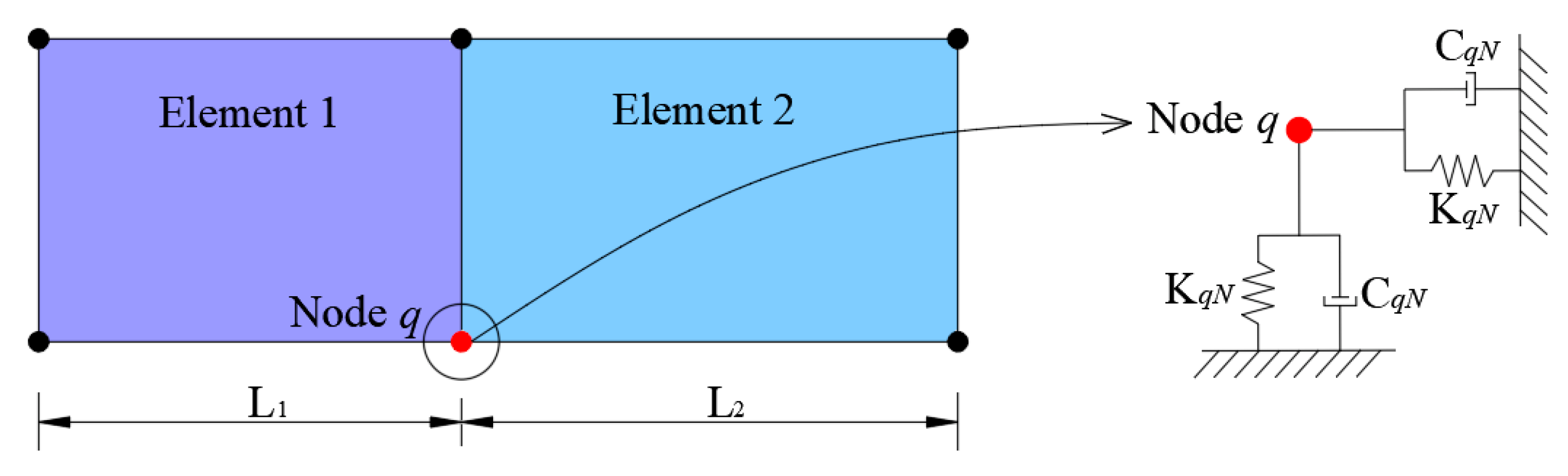
In this paper, the viscoelastic artificial boundary condition is implemented using linear spring-damping elements in ADINA. Figure 1 shows a schematic diagram of a two-dimensional spring-damping element. The stiffness coefficient of the spring element and the damping coefficient of the damper element are:
where and are the normal and tangential stiffness of the spring, respectively; and are the normal and tangential damping coefficients of the damper, respectively; and are the normal and tangential correction coefficients of the viscoelastic artificial boundary, respectively, which are set to and ; and are the wave velocities of the P-wave and S-wave, respectively; and are the shear modulus and mass density of the medium, respectively; is the distance between the wave source and the node on the viscoelastic artificial boundary; is the effective area of the node on the viscoelastic artificial boundary, which usually is the effective length for a two-dimensional finite element model.
3.2. Earthquake Input Mechanisms
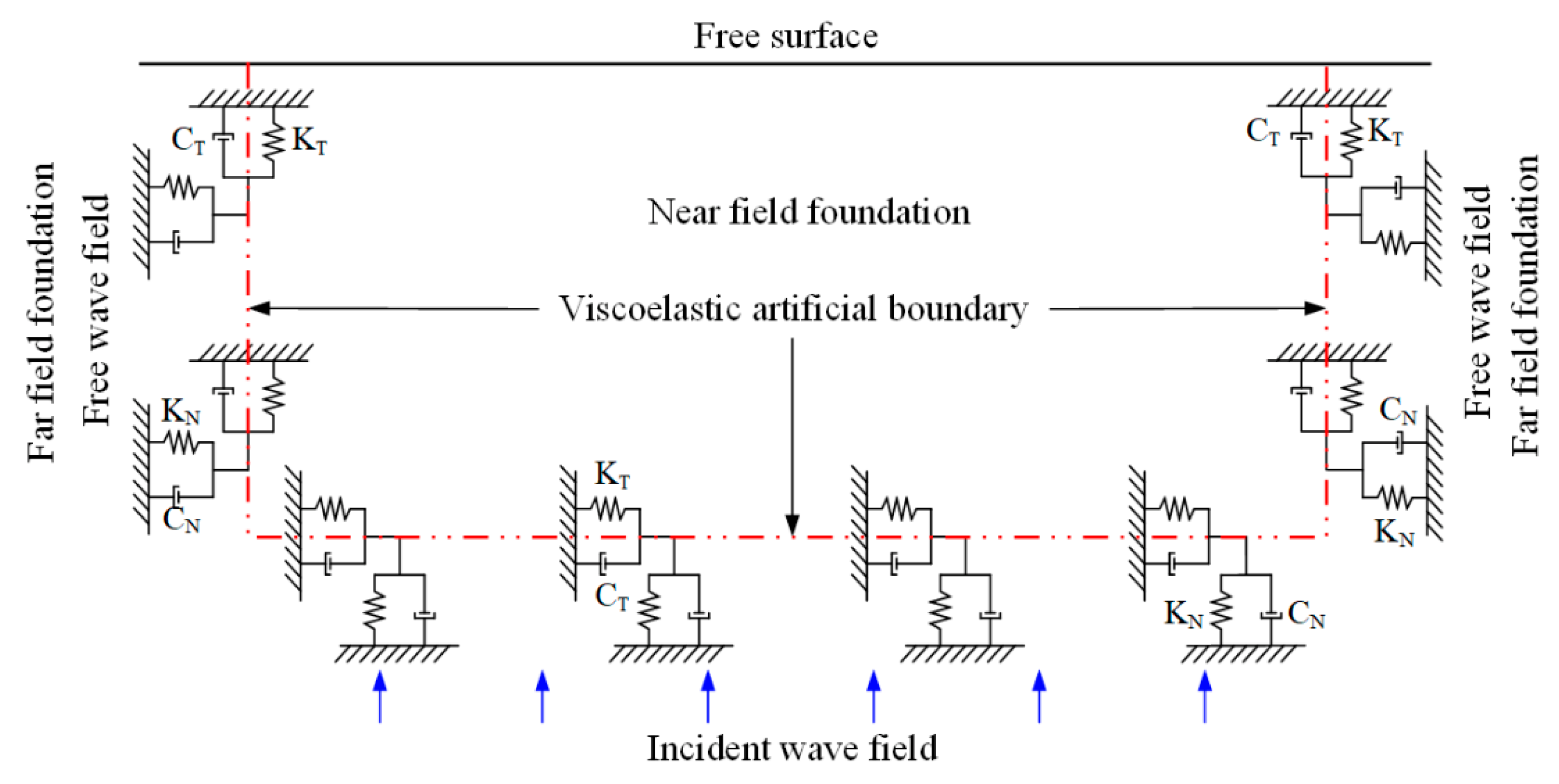
According to the characteristics of wave fields on different viscoelastic artificial boundaries, the total wave field on the bottom boundary is decomposed into an incident field and a scattered field, whereas that on the side boundary is decomposed into a free field and a scattered field. The energy of the scattered field is absorbed by the viscoelastic artificial boundaries, whereas that of incident and free fields can be transformed into equivalent nodal loads and then applied to the boundaries. Figure 2 shows a schematic diagram of wave input for a viscoelastic artificial boundary.
The displacement, velocity, and acceleration time history of wave fields are expressed as , , and , respectively, in which denotes the total wave field, denotes the incident wave field, denotes the free wave field, and denotes the scattered field. According to the displacement continuity condition and the mechanical equilibrium condition, the motion equation for node q on the bottom boundary can be expressed as:
The motion equation for node q on the side boundary can be expressed as:
where and are the artificial boundary parameters of q; , and are the equivalent nodal loads to be applied at q to simulate the incident, free and scattered wave field, respectively. For seismic wave motion input, only equivalent nodal loads and need to be applied to the bottom and side boundary, which are solved using Equations (6) and (7) based on the seismic wave motion propagation pattern and the stress state of wave fields, respectively. The equivalent nodal loads that should be applied at are calculated as follows:
When the primary wave is incident:
When the shear wave vibrating along the Y-axis is incident:
in which
where ρ, cp, cs, λ are the foundation density, P-wave velocity, S-wave velocity, and Lame constant, respectively; Hs is the vertical distance from the wave source to the bottom boundary; h is the vertical distance from q to the bottom boundary; , , , and are the time delay of the incident P-wave at q, the reflected P-wave at the foundation surface, the incident S-wave at q, and the reflected S-wave at the foundation surface, respectively. The subscripts of the equivalent nodal loads represent the node number and component direction, and the superscripts represent the wave field for calculating the equivalent nodal loads and the outer normal direction of the boundary surface at which q is located, which is positive if the direction is the same as the coordinate axis and negative if the direction is opposite to the coordinate axis.
3.3. Verification Test
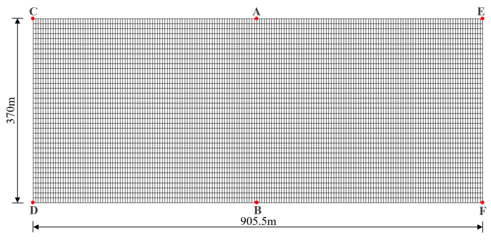
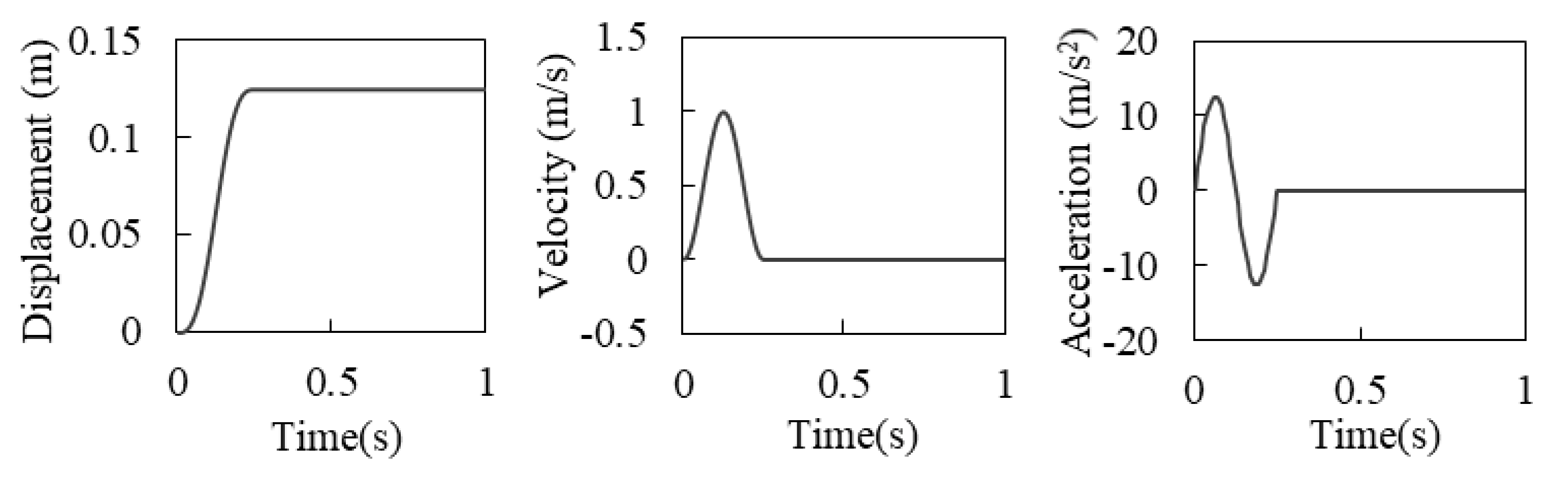
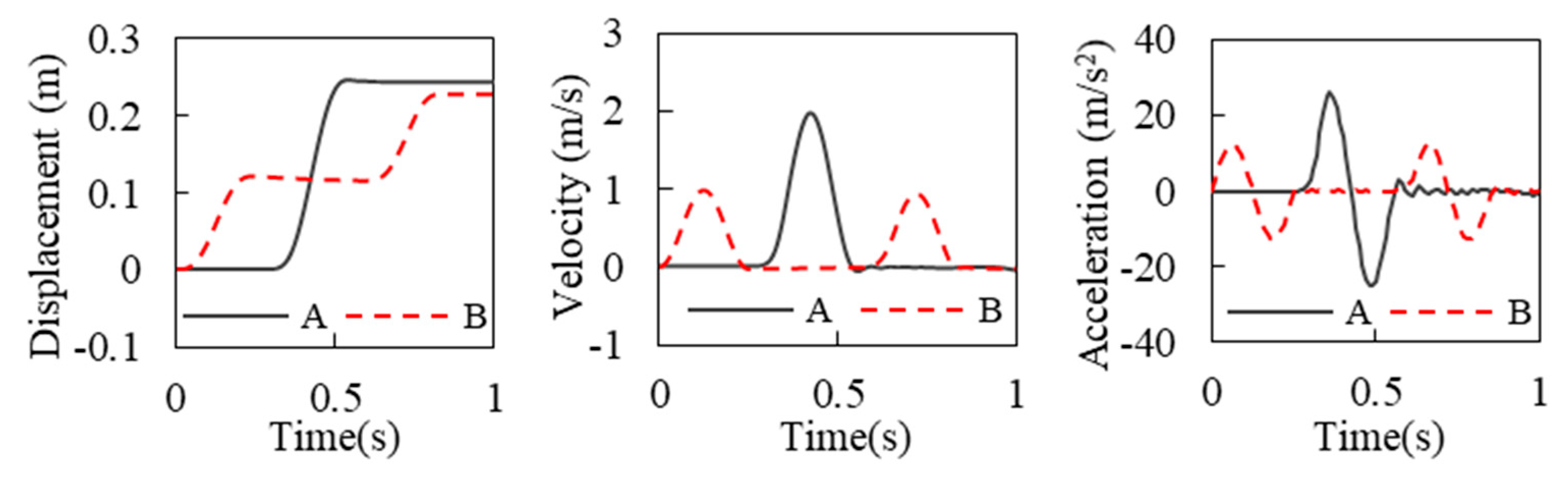
The viscoelastic artificial boundary is verified by a two-dimension test [44]. As shown in Figure 3, the model size is 905.5 m × 370 m, and the finite element mesh size is 5 m × 10 m. The modulus of elasticity of the medium is 1.05 × 10¹⁰ N/m2, the mass density is 2777 kg/m3, the Poisson’s ratio is 0.23, the S-wave velocity is 1239.8 m/s, and the P-wave velocity is 2093.6 m/s. The dynamic time-history analysis is performed with a total calculation time of 1 s and a time step of 0.01 s. The input displacement, velocity, and acceleration time history are determined by Equations (11)–(13) respectively, and their time-history curves are shown in Figure 4.
The time histories of displacement, velocity, and acceleration at each observation point (A and B, C and D, E and F in Figure 3) are calculated. Figure 5 shows the time history curves of horizontal displacement, velocity, and acceleration at position A on the free surface and position B on the bottom boundary directly below position A. It is seen that the seismic wave is input from the bottom truncated boundary, and the amplitude of the seismic wave is doubled when the incident wave reaches the free surface. The seismic wave reflected from the free surface is absorbed by the viscoelastic boundary after reaching the bottom surface, without reflection on the truncated boundary. Similar dynamic responses are observed at other observation positions (C and D, E and F). These results indicate that the viscoelastic artificial boundary condition and the corresponding earthquake input mechanism are feasible.
4. General Description of the Numerical Example
4.1. General Information
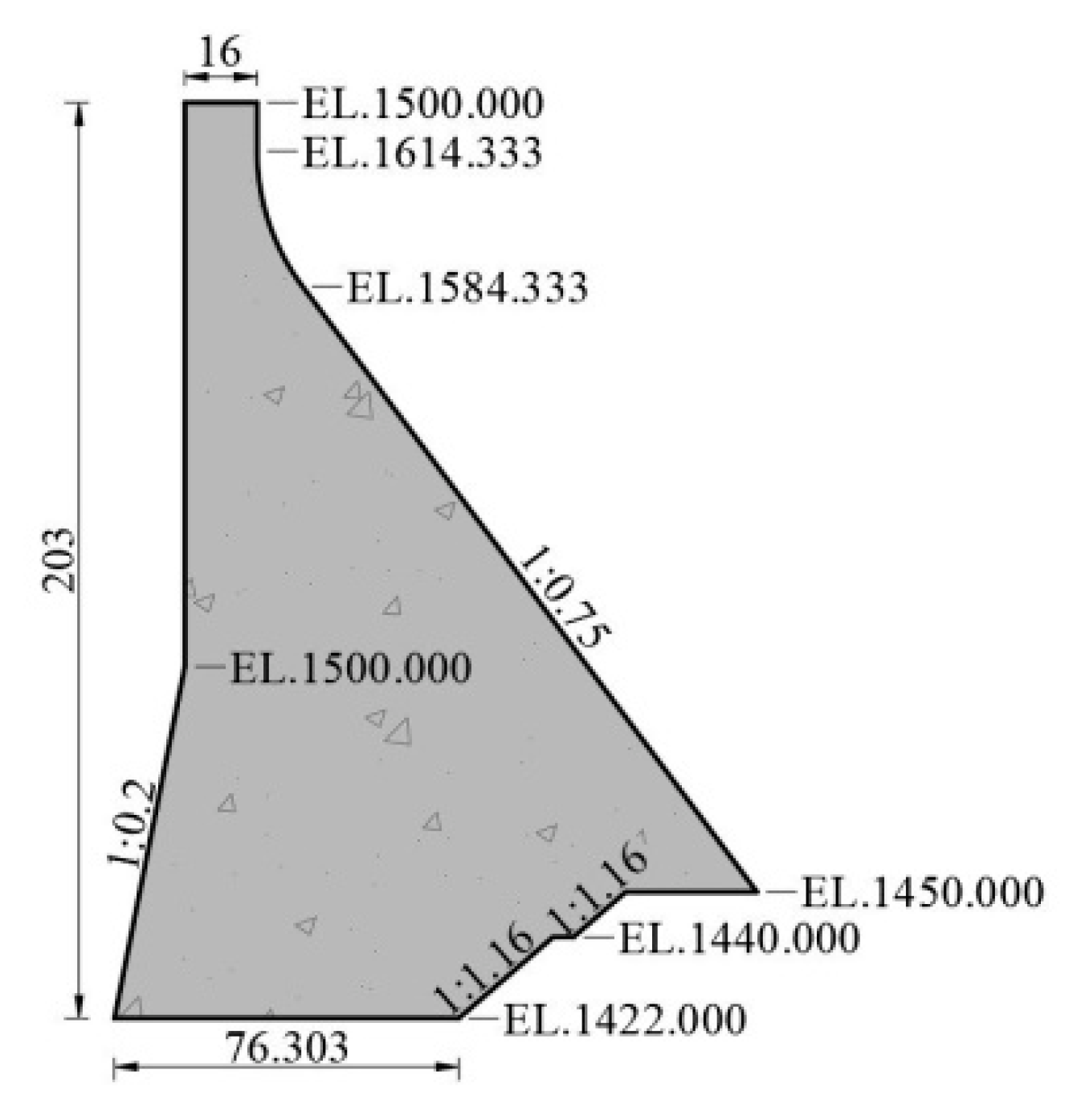
A concrete gravity dam in Southwest China was selected as the study case. The concrete gravity dam block has a crest elevation of 1625 m, a heel elevation of 1422 m, a dam height of 203 m, a crest width of 16 m, and a normal water level of 1619 m. The calculation cross-section of the dam block is shown in Figure 6. In this study, the following material parameters were considered. Dam: static modulus of elasticity = 2.5 × 10¹⁰ N/m2, mass density = 2400 kg/m3, Poisson’s ratio = 0.167 according to Design Code for Hydraulic Concrete Structures (SL 191-2008) [45], structural damping = 5%. Foundation: modulus of elasticity = 1.5 × 10¹⁰ N/m2, mass density = 2700 kg/m3, Poisson’s ratio = 0.24. Reservoir: mass density of water = 1000 kg/m3, acoustic wave speed = 1440 m/s.
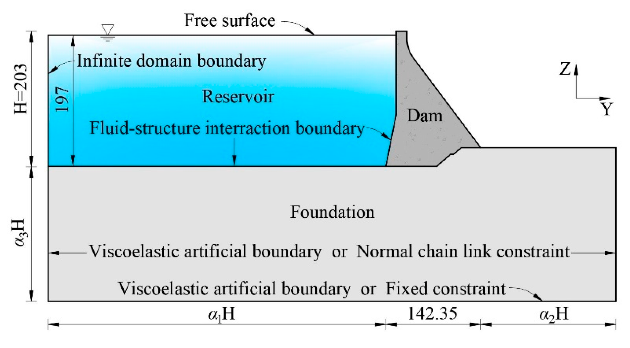
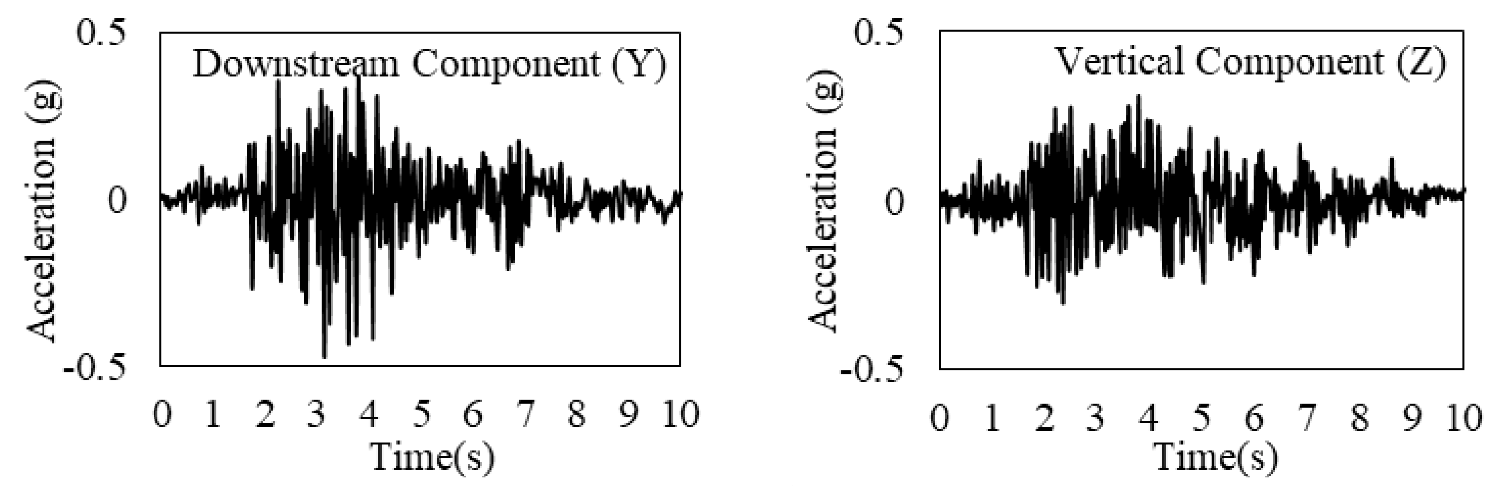
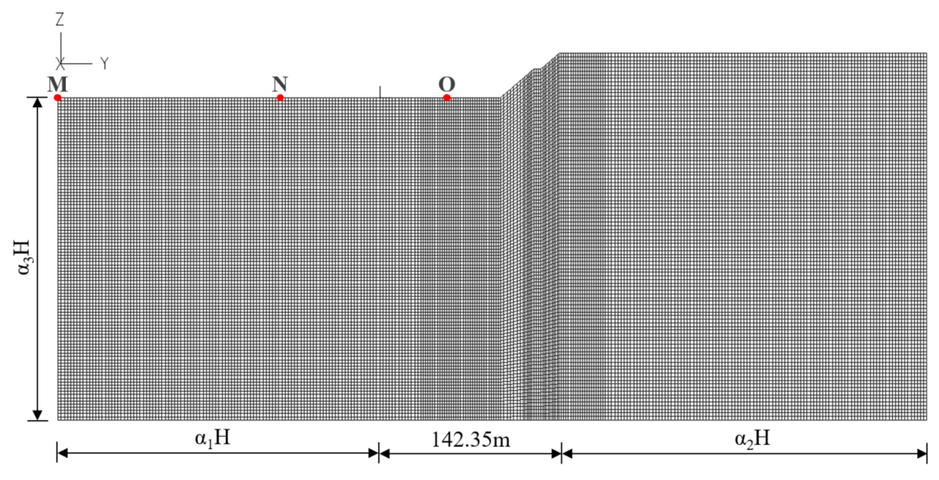
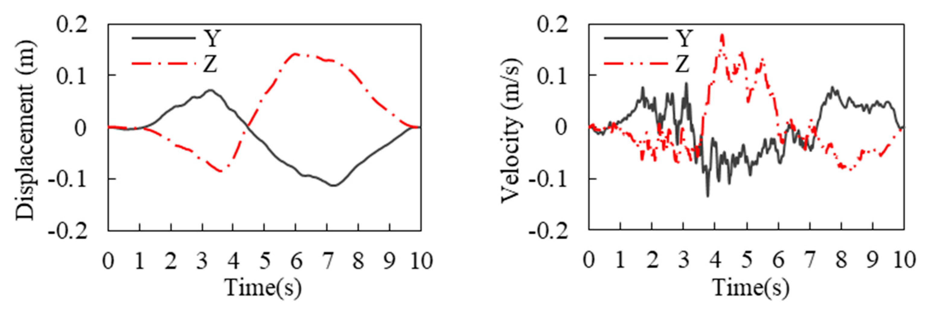
The geometry of the dam–foundation–reservoir system is shown in Figure 7. The mesh size of the two-dimension finite element model was controlled to be about 2 m × 2 m. The dam was simulated with 4640 plane stress elements, and the foundation was simulated with 207,900 plane strain elements. Both static and dynamic effects were taken into account by the static–dynamic superposition method. The loads include the self-weight, hydrostatic pressure, hydrodynamic pressure, and seismic load, where the hydrodynamic pressure is simulated by added mass or potential-based fluid elements. The acceleration record of Koyna earthquake with the United States Geological Survey (USGS) site classification of A and the magnitude of 6.3 M was selected as the seismic loading, the site of which is similar to the example dam. Figure 8 shows the Koyna earthquake acceleration time history, and only downstream (Y) and vertical (Z) ground motions are considered in the calculations, where the PGA in the Y and Z direction is 0.474 g and 0.304 g, respectively.
4.2. Cases of the Numerical Analysis
A series of cases were designed to identify factors affecting the dynamic response of concrete gravity dams, such as the simulation method of the foundation, foundation size, radiation damping effect, compressibility of reservoir water, and reservoir water length. Table 1 summarizes the dam–foundation–reservoir finite element models used for all cases, where RF = rigid foundation, MLF = massless foundation, VABF = foundation with viscoelastic artificial boundary, WAMR = reservoir water simulated by the Westergaard added mass method, IPFR = reservoir water simulated by incompressible potential-based fluid elements, and CPFR = reservoir water simulated by compressible potential-based fluid elements.
5. Dynamic Characteristics
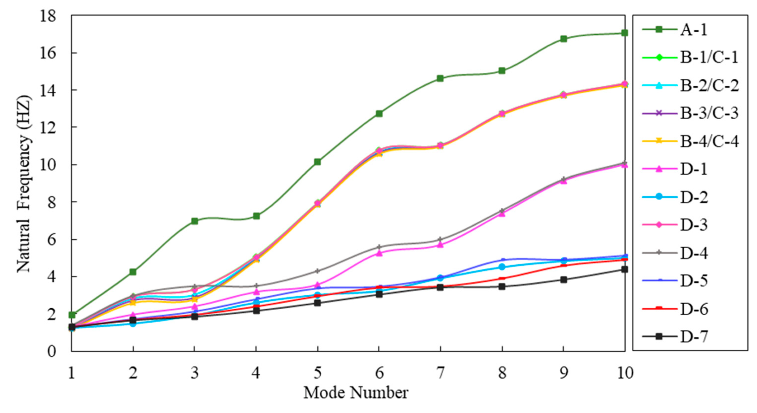
The foundation is assumed to be massless in all cases, and thus case B is the same as case C in modal analyses. A fixed constraint is applied to the bottom boundary of the foundation and a normal chain link constraint is applied to the side boundary. A zero potential boundary condition is set at the reservoir free surface [46], the infinite domain boundary condition is applied at the far end of reservoir, and the fluid–solid coupling boundary conditions are set at the interfaces of reservoir–dam and reservoir–foundation. The first 10 natural frequencies of the dam are listed in Table 2, and their distributions are shown in Figure 9.
In cases A and B, the hydrodynamic pressure of reservoir water is simulated by the added mass method considering only the unidirectional effect of reservoir water on the dam. It is found that in case A in which the RF model is used without considering the dam–foundation interaction, the natural frequency is the highest in all cases and the 10th natural frequency is about 9 times that of the first one. In cases B in which the dam–foundation interaction is considered, the first 10 natural frequencies are greatly reduced. Compared with the RF model, the first three natural frequencies of the MLF model are reduced by about 35%, 35%, and 57%, respectively. Comparison of cases B-1, B-2, B-3, and B-4 shows that the natural frequency decreases with the increase in foundation size, which appears to be more pronounced for low-order natural frequencies. The first natural frequency on the foundation with a size of 3H is reduced by 7.12% compared that with the size of 1 H, whereas the 10th natural frequency is reduced by only 0.44%.
In cases D, except D-3, reservoir water is simulated using potential-based fluid elements considering the dam–foundation–reservoir dynamic interaction. Comparing C-4, D-1, and D-2, it is found that the WAMR model gives the highest natural frequencies of the dam, followed by the IPFR model and then the CPFR model, and the difference increases as the mode number increases. As a result, the 10th natural frequency of the CPFR model is about 65% lower than that of the WAMR model. The simulation methods of reservoir water may have an effect on the increase in the natural frequency with the mode number. The highest increase is achieved by the WAMR model, and it is decreased by 30% for the IPFR model and by 70% for the CPFR model. It is seen in cases D-5, D-6, and D-7 that increasing the reservoir water length has little effect on the first three natural frequencies, but a greater effect on the higher order natural frequencies. The first natural frequencies are basically the same for models of 3H and 5H, but the 10th natural frequency for models of 5H are reduced by 14.43% compared with that of 3H.
Thus, it is concluded that the natural frequency of the dam decreases greatly when the dam–foundation interaction is considered, and decreases slightly with the increase in the foundation size. The simulation methods of reservoir water have significant effects on the natural frequency of the dam, whereas the reservoir water lengths have no obvious effect.
6. Dam-Foundation Interaction
6.1. Simulation Methods of Foundation
In this study, the RF, MLF, and VABF models were used to analyze the effects of different foundation simulation methods on the dynamic response of concrete gravity dams. Table 3 lists the extreme values of dynamic responses for the three simulation methods, in which the acceleration magnification factor is the multiple of the maximum acceleration of the dam crest over the maximum input acceleration, and the relative displacement is obtained by subtracting the displacement of the dam heel from that of the dam crest.
As can be seen from Table 3, the RF model gives the largest acceleration response, and the acceleration is reduced by about 30% for the MLF model and 65% for the VABF model. The MLF model gives the maximum relative displacement of the dam crest, as it takes into account the elasticity of the foundation, and the deformation of the foundation during the earthquake may tilt the gravity dam as a whole. Compared with the VABF model, the radiation damping effect of the infinite foundation is not adequately considered in the MLF model. For the RF model, the maximum values of vertical normal tensile and compressive stress appear at the slope of the upstream dam face with little difference, whereas the maximum values of vertical normal tensile and compressive stress appear at the dam heel for both MLF and VABF models, and the vertical normal compressive stress is significantly larger than the vertical normal tensile stress. The RF model gives the lowest principal tensile and compressive stress of the dam, and the maximum principal tensile stress appears at the dam heel and the maximum principal compressive stress appears at the neck of the downstream dam face. For both MLF and VABF models, the maximum principal tensile stress appears at the dam heel, and the maximum principal compressive stress appears at the dam toe. However, it is noted that the maximum principal tensile stress under the VABF model is smaller than that under the MLF model.
6.2. Sensitivity Analysis of Foundation Size
Cases B-1, B-2, B-3, and B-4 with different foundation sizes (1H, 1.5H, 2H, and 3H in the upstream, downstream and depth directions) were analyzed to elucidate their effects on the dynamic response of gravity dams. Each of the four cases were modeled with the MLF model and calculated by applying fixed constraints to the bottom boundary of the foundation and normal chain link constraints to the side boundary. The hydrodynamic pressure of reservoir water was simulated by the added mass method. Table 4 lists the extreme values of dam dynamic responses under for different foundation sizes.
Table 4 clearly shows that foundation size has a significant effect on the acceleration response. Specifically, the downstream acceleration at the dam crest reaches a maximum at a foundation size of 2H, which is 5.789 times that of the input; and a minimum at a foundation size of 3H, which is 3.477 times that of the input. The vertical acceleration at the dam crest reaches a maximum at a foundation size of 3H, which is 4.220 times that of the input. However, foundation size has little effect on displacement, and both downstream and vertical relative displacement at the dam crest reach a maximum at a foundation size of 2H. The tensile stress can also be significantly affected by foundation size, and the maximum tensile stress decreases with the increase in foundation sizes. As a result, the maximum vertical normal tensile stress and the maximum principal tensile stress at a foundation size of 3H are decreased by about 26.8% and 35.9% compared with that at a foundation size of 1H, respectively.
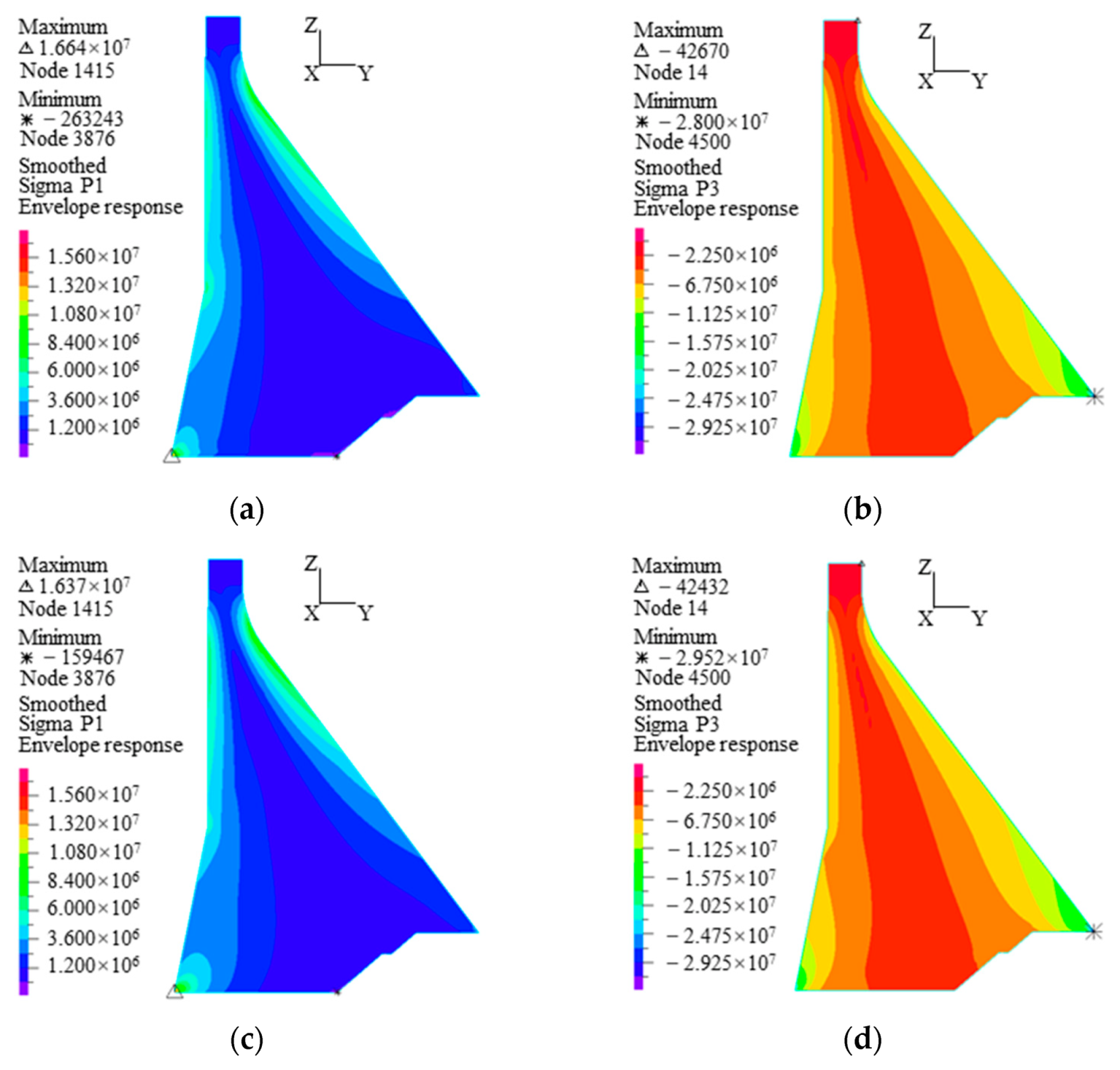
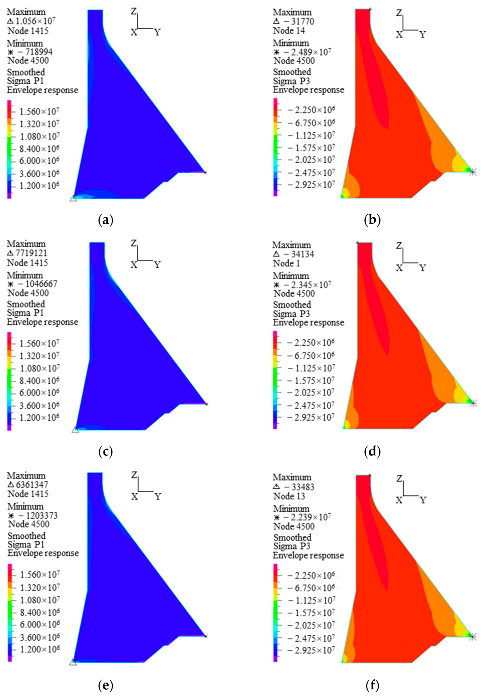
Figure 10 shows the principal stress envelopes of the dam in the four cases. It is found that foundation size has little effect on the distributions of principal tension and compression stress, and in all cases, the maximum principal tension stress appears at the dam heel and the maximum principal compressive stress appears at the dam toe.
6.3. The Radiation Damping Effect of Infinite Foundation
6.3.1. Verification of the Foundation Model
The finite element model of the foundation (Figure 11) was analyzed using the method described in Section 3. The foundation sizes were also assumed to be 1H, 1.5H, 2H, and 3H, and the material properties are described in Section 4. The sinusoidal waves given by Equations (11)–(13) are input from the bottom boundary of the foundation with a peak of 12.542 m/s2 in both downstream and vertical directions. Three observation points are set on the foundation surface: point M which is closest to the upstream side, point N which is the intermediate point of the upstream side, and point O where there is the wave source. The PGA values at these three points are listed in Table 5. It is seen that the amplitude of the wave is almost doubled when it reaches the free surface of the foundation, which is consistent with the theory and further verifies the applicability of the viscoelastic artificial boundary and corresponding earthquake input mechanism.
The Koyna earthquake record was used to further verify the foundation model. It was found that the input from the bottom boundary of the foundation is folded in half, with a PGA of 2.324 m/s2 in the downstream direction and 1.528 m/s2 in the vertical direction. The displacement and velocity time histories are given in Figure 12, and the PGA values at each observation point are shown in Table 6.
Theoretically, the PGA at the observation points should be twice that of the input as the seismic excitation is transmitted to the foundation surface. However, Table 6 shows that there are some discrepancies between the theoretical and observed PGAs, and in general the error is the smallest for the foundation with a size of 3H.
6.3.2. The Radiation Damping Effect
In contrast with the results of the MLF model in Section 6.2, four cases C-1, C-2, C-3, and C-4, which have the same foundation sizes as cases B-1, B-2, B-3, and B-4, respectively, were designed and analyzed. The viscoelastic artificial boundary condition is applied at the truncation boundary of the foundation, and the hydrodynamic pressure of reservoir water is simulated by added mass.
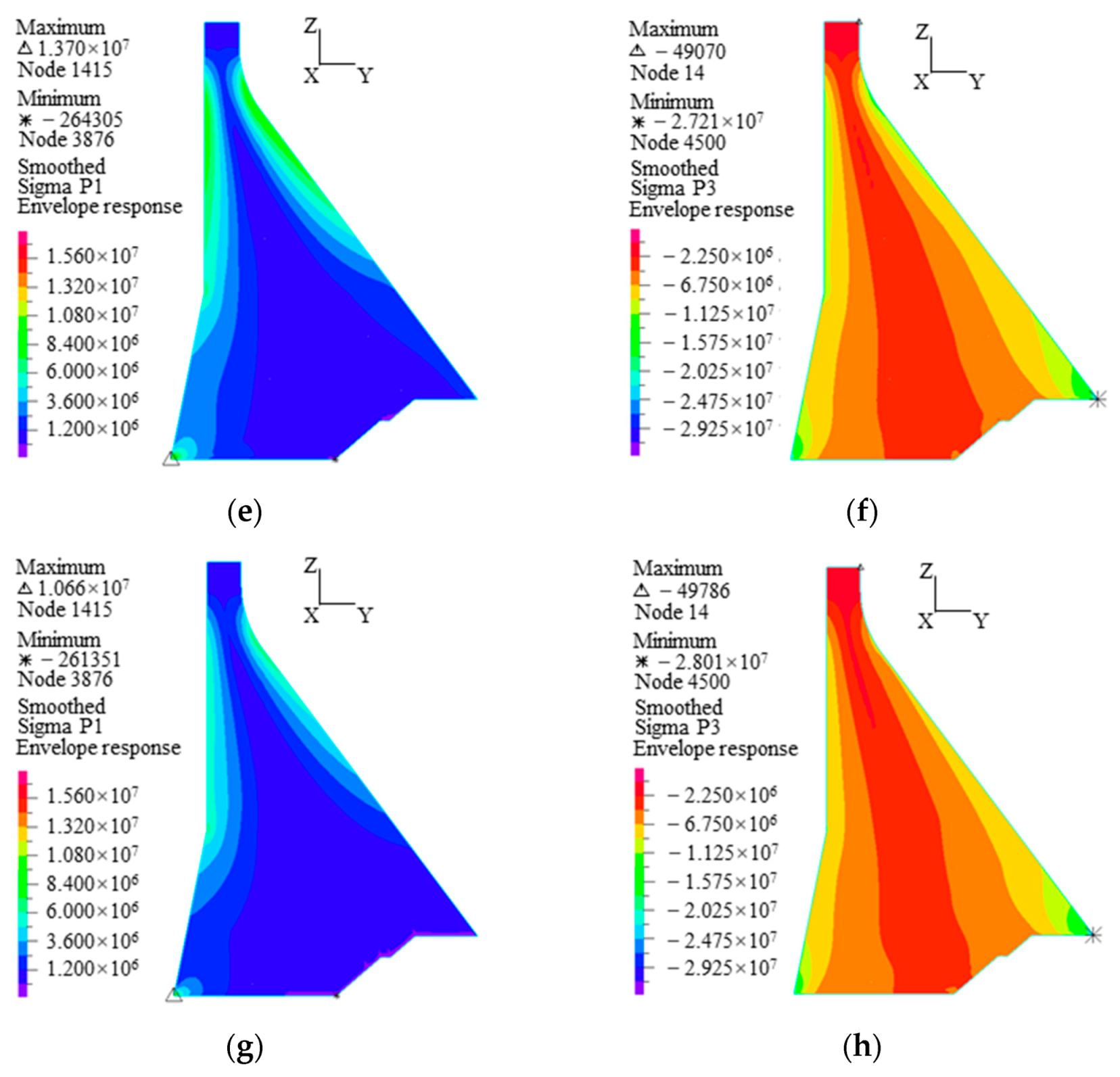
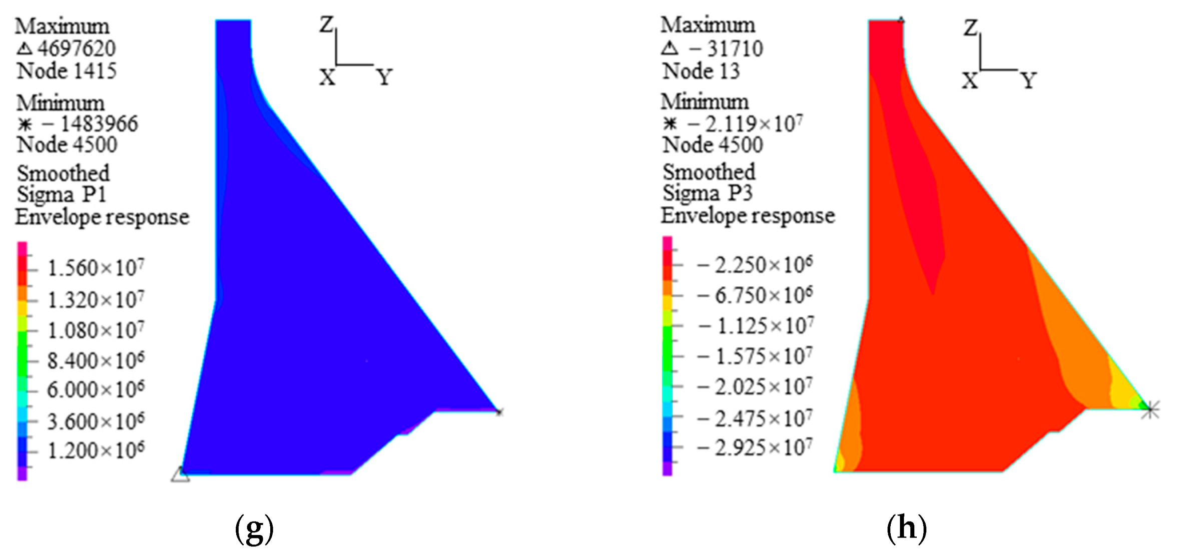
Comparison between Table 7 and Table 4 indicates that the dynamic responses of the dam obtained using the VABF model are significantly smaller than those obtained using the MLF model. Specifically, the VABF model leads to 45–67% reductions in acceleration, 38–50% reductions in displacement, 28–56% reductions in principal tensile stress, and 11–24% reductions in principal compressive stress. Figure 13 shows the principal stress envelopes of the dam at different foundation sizes obtained using the VABF model. As compared with Figure 10, the high stress zone is significantly reduced, indicating that more conservative dynamic responses are obtained by the MLF model, whereas the dam dynamic responses can be reduced effectively when the VABF model is used.
Table 7 shows that the downstream acceleration at the dam crest decreases as the foundation size increases, and the minimum acceleration is 1.910 times that of the input at a foundation size of 3H. The vertical acceleration is 1.654 times that of the input at a foundation size of 2H and 3H. However, the relative displacement at the dam crest is less affected by foundation size. The downstream relative displacement decreases slightly with the increase in foundation size, and the displacement at a foundation size of 3H is 25.4% lower than that at a foundation size of 1H. It should be noted that the tensile and compressive stresses of the dam decrease most significantly with the increase in foundation size. As a result, the foundation size of 3H leads to a 22.1% decrease in the maximum vertical normal tensile stress, a 20.2% decrease in the maximum vertical normal compressive stress, a 55.5% decrease in the maximum principal tensile stress, and a 14.9% decrease in the maximum principal compressive stress compared to the foundation size of 1H.
7. Dam–Reservoir Interaction
7.1. Simulation Methods of Reservoir
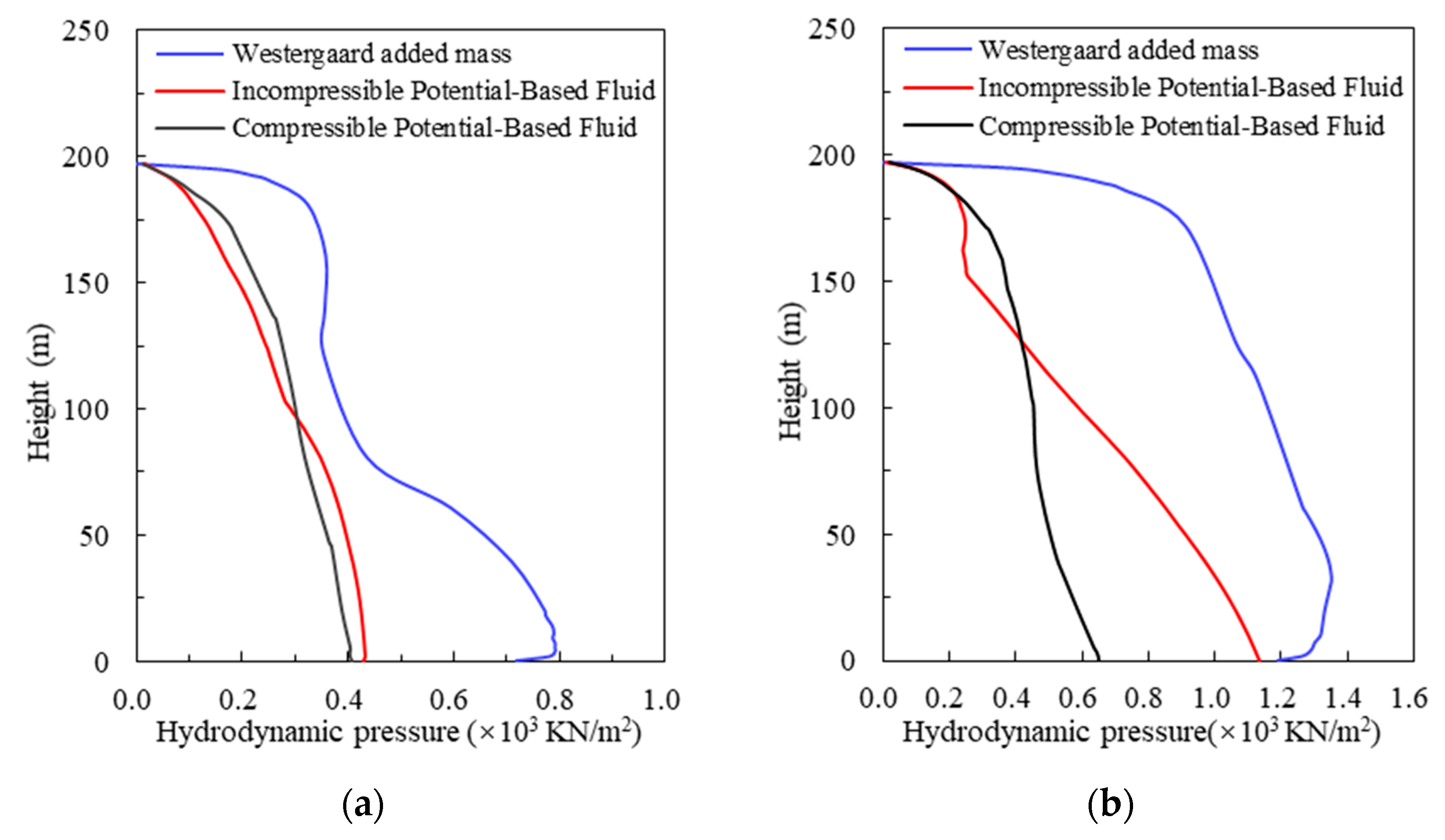
In the above cases, the hydrodynamic pressure of reservoir water was simulated using the Westergaard added mass method without considering its compressibility. In order to deal with this problem, the potential-based fluid elements in ADINA were used to simulate the incompressible and compressible reservoir water, as presented in this section. Accordingly, the free surface boundary condition is applied on the reservoir surface, the infinite domain boundary condition is applied at the far end of the reservoir, and the fluid–solid coupling boundary condition is applied at the junctions of reservoir–dam and reservoir–foundation. Table 8 shows the extreme values of dam dynamic responses in the six cases, and Figure 14 shows the distributions of maximum hydrodynamic pressure along the dam–reservoir interface obtained by different reservoir simulation methods.
According to Table 8, the reservoir water simulation methods have no significant effects on the acceleration and displacement of the dam, but have significant effects on the stress. The Westergaard added mass method leads to a significant reduction in the vertical normal tensile stress at the dam heel, because it only considers the unidirectional effect of reservoir water on the dam and thus neglects the movement of reservoir water and its interaction with the foundation. In contrast, the potential-based fluid simulation method takes into account both reservoir–dam and reservoir–foundation interactions. Under the influence of gravity, the hydrodynamic pressure is applied to the upstream foundation surface as the reservoir water flows, which may cause downward deformation of the foundation and consequently affect the normal tensile stress at the dam heel. The maximum principal tensile stress of the dam appears at the dam heel. It is noted that when the VABF model is used, the maximum principal tensile stress of the CPFR model is 15% higher than that of the IPFR model, which is approximately 3 times that of the WAMR model, whereas when the MLF model is used, the maximum principal tensile stress of the CPFR model is 19% higher than that of the IPFR model and 24% higher than that of the WAMR model. The maximum principal compressive stress of the dam appears at the dam toe, and is less affected by the reservoir water simulation methods. When the VABF model is used, the maximum principal compressive stress of the CPFR model is 8% lower than that of the WAMR model but 2% higher than that of the IPFR model, whereas when the MLF model is used, the maximum principal compressive stress of the CPFR model is 12% lower than that of the WAMR model but 10% higher than that of the IPFR model. As shown in Figure 14, the hydrodynamic pressure along the dam–reservoir interface of the WAMR model is significantly higher compared to the other two models. Below 100 m, the hydrodynamic pressure of the IPFR model is significantly higher than that of the CPFR model.
7.2. Reservoir Water Length
As presented in this section, reservoir water with a length of 3H, 4H, and 5H [47] was simulated using compressible potential-based fluid elements to investigate its effect on the dynamic response of the dam, and the extreme values of dynamic responses are given in Table 9.
The results show that the reservoir water length of 3H leads to a 7–23% increase in acceleration, a 9–33% increase in displacement, a 15–18% increase in the maximum principal tensile stress, a 3–6% increase in the maximum principal compressive stress, and a 41–61% increase in the maximum hydrodynamic pressure at the dam heel compared to the reservoir water length of 4H and 5H.
8. Conclusions
In this study, some key factors, such as the dynamic interactions of dam–foundation and dam–reservoir, were considered in the dynamic numerical analysis of a 200 m high gravity dam. The rigid, massless, and viscoelastic artificial boundary foundation models were established to account for the effect of dam–foundation dynamic interaction on the dynamic responses of the dam. Three reservoir water simulation methods, namely, the Westergaard added mass method, and the incompressible and compressible potential fluid methods, were used to account for the effect of hydrodynamic pressure on the dynamic characteristics of the dam. The ranges of the truncation boundary of the foundation and reservoir in numerical analysis were further investigated. The following conclusions can be drawn:
- (1)
- The natural frequency of the dam decreases greatly in numerical analysis when the dam–foundation interaction is considered, and decreases slightly with the increase in the foundation size. The simulation methods of reservoir water have significant effects on the natural frequency of the dam, whereas the reservoir water lengths have no significant effect.
- (2)
- The dynamic interaction of the dam and the foundation cannot be ignored. The radiation damping effect should be considered in the dynamic numerical analysis. The viscoelastic artificial boundary foundation is more efficient than the massless foundation in simulating the radiation damping effect of the far-field foundation. It was found that a foundation range of 3 times the dam height in all directions, such as upstream, downstream, and depth, is the most reasonable range of the truncation boundary of the foundation.
- (3)
- The methods used for reservoir water simulation have no significant effects on the acceleration and displacement of the dam, but have a significant effect on the stress. Compared with the Westergaard added mass method, the potential-based fluid simulation method simultaneously takes into account the reservoir–dam and reservoir–foundation interactions. The static and dynamic water pressure was applied to the upstream foundation surface as the reservoir water, which may cause downward deformation of the foundation and consequently increase the normal tensile stress at the dam heel. It was found that a reservoir length of 3 times the dam height is feasible for the truncation boundary of the reservoirs.
Author Contributions
Conceptualization, H.Z.; methodology, H.Z.; validation, C.W., Y.Z., Y.W. and T.T.T.H.; resources, H.Z. and L.G.; data curation, C.W.; writing—original draft preparation, C.W.; writing—review and editing, H.Z. and C.W.; supervision, H.Z., L.G., Y.W. and T.T.T.H. All authors have read and agreed to the published version of the manuscript.
Funding
This work was supported by the Open Research Fund of State Key Laboratory of Simulation and Regulation of Water Cycle in River Basin (China Institute of Water Resources and Hydropower Research) (grant number IWHR-SKL-KF201816), the National Key Research and Development Program of China (grant number 2017YFC0404903), and the Natural Science Foundation of Jiangsu Province (grant number BK20170884).
Institutional Review Board Statement
Not applicable.
Informed Consent Statement
Not applicable.
Data Availability Statement
The data presented in this study are available on request from the corresponding author.
Conflicts of Interest
The authors declare that they have no known competing financial interests or personal relationships that could have appeared to influence the work reported in this paper.
References
- Ghaedi, K.; Hejazi, F.; Ibrahim, Z.; Khanzaei, P. Flexible foundation effect on seismic analysis of roller compacted concrete (RCC) dams using finite element method. KSCE J. Civ. Eng. 2017, 22, 1275–1287. [Google Scholar] [CrossRef]
- Bayraktar, A.; Hançer, E.; Akköse, M. Influence of base-rock characteristics on the stochastic dynamic response of dam–reservoir–foundation systems. Eng. Struct. 2005, 27, 1498–1508. [Google Scholar] [CrossRef]
- Ghaemian, M.; Noorzad, A.; Mohammadnezhad, H. Assessment of foundation mass and earthquake input mechanism effect on dam–reservoir–foundation system response. Int. J. Civ. Eng. 2019, 17, 473–480. [Google Scholar] [CrossRef]
- Salamon, J.W.; Wood, C.; Hariri-Ardebili, M.A.; Malm, R.; Faggiani, G. Seismic Analysis of Pine Flat Concrete Dam: Formulation and Synthesis of Results; Springer International Publishing: Cham, Switzerland, 2020; pp. 3–97. [Google Scholar]
- Chopra, A. Earthquake analysis of concrete dams: Factors to be considered. In Proceedings of the Proceedings of the 10th National Conference in Earthquake Engineering, Anchorage, AK, USA, 21–25 July 2014. [Google Scholar]
- Hariri-Ardebili, M.A.; Kolbadi, S.M.S.; Kianoush, M. FEM-based parametric analysis of a typical gravity dam considering input excitation mechanism. Soil Dyn. Earthq. Eng. 2016, 84, 22–43. [Google Scholar] [CrossRef]
- Hariri-Ardebili, M.A.; Mirzabozorg, H. A comparative study of seismic stability of coupled arch dam-foundation-reservoir systems using infinite elements and viscous boundary models. Int. J. Struct. Stab. Dyn. 2013, 13, 1350032. [Google Scholar] [CrossRef]
- Burman, A.; Nayak, P.; Agrawal, P.; Maity, D. Coupled gravity dam–foundation analysis using a simplified direct method of soil–structure interaction. Soil Dyn. Earthq. Eng. 2012, 34, 62–68. [Google Scholar] [CrossRef]
- Wang, H.; Feng, M.; Yang, H. Seismic nonlinear analyses of a concrete gravity dam with 3D full dam model. Bull. Earthq. Eng. 2012, 10, 1959–1977. [Google Scholar] [CrossRef]
- Lysmer, J.; Kuhlemeyer, R.L. Finite dynamic model for infinite media. J. Eng. Mech. Div. 1969, 95, 859–878. [Google Scholar] [CrossRef]
- Hariri-Ardebili, M.A. Impact of foundation nonlinearity on the crack propagation of high concrete dams. Soil Mech. Found. Eng. 2014, 51, 72–82. [Google Scholar] [CrossRef]
- Liu, J.; Du, Y.; Du, X.; Wang, Z.; Wu, J. 3D viscous-spring artificial boundary in time domain. Earthq. Eng. Eng. Vib. 2006, 5, 93–102. [Google Scholar] [CrossRef]
- Liang, H.; Tu, J.; Guo, S.; Liao, J.; Li, D.; Peng, S. Seismic fragility analysis of a High Arch Dam-Foundation System based on seismic instability failure mode. Soil Dyn. Earthq. Eng. 2020, 130, 105981. [Google Scholar] [CrossRef]
- Song, C.; Wolf, J.P. The scaled boundary finite-element method—alias consistent infinitesimal finite-element cell method—for elastodynamics. Comput. Methods Appl. Mech. Eng. 1997, 147, 329–355. [Google Scholar] [CrossRef]
- Qu, Y.; Chen, D.; Liu, L.; Ooi, E.T.; Eisenträger, S.; Song, C. A direct time-domain procedure for the seismic analysis of dam–foundation–reservoir systems using the scaled boundary finite element method. Comput. Geotech. 2021, 138, 104364. [Google Scholar] [CrossRef]
- Hariri-Ardebili, M.A.; Kianoush, M. Integrative seismic safety evaluation of a high concrete arch dam. Soil Dyn. Earthq. Eng. 2014, 67, 85–101. [Google Scholar] [CrossRef]
- Basu, U.; Chopra, A.K. Erratum to‘Perfectly matched layers for transient elastodynamics of unbounded domains’(Int. J. Numer. Meth. Engng 2004; 59:1039–1074). Int. J. Numer. Methods Eng. 2004, 61, 156–157. [Google Scholar] [CrossRef]
- Harirri-Ardebili, M.A.; Saouma, V.E. Impact of near-fault vs. far-field ground motions on the seismic response of an arch dam with respect to foundation type. Dam Eng. 2013, 24, 19–52. [Google Scholar]
- Pan, J.W.; Song, C.M.; Zhang, C.H. Simple model for gravity dam response considering radiation damping effects. J. Hydraul. Eng. 2010, 41, 493–498. [Google Scholar] [CrossRef]
- Chen, D.; Hou, C.; Wang, F. Influences on the seismic response of the gravity dam-foundation-reservoir system with different boundary and input models. Shock. Vib. 2021, 2021, 1–15. [Google Scholar] [CrossRef]
- Wang, G.; Wang, Y.; Lu, W.; Zhou, C.; Chen, M.; Yan, P. XFEM based seismic potential failure mode analysis of concrete gravity dam–water–foundation systems through incremental dynamic analysis. Eng. Struct. 2015, 98, 81–94. [Google Scholar] [CrossRef]
- Wang, G.; Wang, Y.; Lu, W.; Yan, P.; Zhou, W.; Chen, M. A general definition of integrated strong motion duration and its effect on seismic demands of concrete gravity dams. Eng. Struct. 2016, 125, 481–493. [Google Scholar] [CrossRef]
- Gorai, S.; Maity, D. Seismic response of concrete gravity dams under near field and far field ground motions. Eng. Struct. 2019, 196, 109292. [Google Scholar] [CrossRef]
- Chen, D.-H.; Yang, Z.-H.; Wang, M.; Xie, J.-H. Seismic performance and failure modes of the Jin’anqiao concrete gravity dam based on incremental dynamic analysis. Eng. Fail. Anal. 2019, 100, 227–244. [Google Scholar] [CrossRef]
- Asghari, E.; Taghipour, R.; Bozorgnasab, M.; Moosavi, M. Seismic analysis of concrete gravity dams considering foundation mass effect. KSCE J. Civ. Eng. 2018, 22, 4988–4996. [Google Scholar] [CrossRef]
- Mirzabozorg, H.; Akbari, M.; Hariri-Ardebili, M.A. Wave passage and incoherency effects on seismic response of high arch dams. Earthq. Eng. Eng. Vib. 2012, 11, 567–578. [Google Scholar] [CrossRef]
- Westergaard, H.M. Water pressures on dams during earthquakes. Trans. Am. Soc. Civ. Eng. 1933, 98, 418–433. [Google Scholar] [CrossRef]
- Khiavi, M.P.; Sari, A. Evaluation of hydrodynamic pressure distribution in reservoir of concrete gravity dam under vertical vibration using an analytical solution. Math. Probl. Eng. 2021, 2021, 1–9. [Google Scholar] [CrossRef]
- Amina, T.B.; Mohamed, B.; André, L.; Abdelmalek, B. Fluid–structure interaction of Brezina arch dam: 3D modal analysis. Eng. Struct. 2015, 84, 19–28. [Google Scholar] [CrossRef]
- Altunişik, A.C.; Sesli, H. Dynamic response of concrete gravity dams using different water modelling approaches: Westergaard, lagrange and euler. Comput. Concr. 2015, 16, 429–448. [Google Scholar] [CrossRef]
- Altunisik, A.C.; Sesli, H.; Hüsem, M.; Akköse, M. Performance Evaluation of gravity dams subjected to near- and far-fault ground motion using Euler approaches. Iran. J. Sci. Technol. Trans. Civ. Eng. 2018, 43, 297–325. [Google Scholar] [CrossRef]
- Bayraktar, A.; Türker, T.; Akköse, M.; Ateş, Ş. The effect of reservoir length on seismic performance of gravity dams to near- and far-fault ground motions. Nat. Hazards 2010, 52, 257–275. [Google Scholar] [CrossRef]
- Kartal, M.E.; Cavusli, M.; Sunbul, A.B. Assessing seismic response of a 2D roller-compacted concrete dam under variable reservoir lengths. Arab. J. Geosci. 2017, 10, 488. [Google Scholar] [CrossRef]
- Pelecanos, L.; Kontoe, S.; Zdravković, L. Numerical modelling of hydrodynamic pressures on dams. Comput. Geotech. 2013, 53, 68–82. [Google Scholar] [CrossRef] [Green Version]
- Mandal, K.; Maity, D. Transient response of concrete gravity dam considering dam-reservoir-foundation interaction. J. Earthq. Eng. 2016, 22, 211–233. [Google Scholar] [CrossRef]
- Løkke, A.; Chopra, A.K. Direct finite element method for nonlinear earthquake analysis of 3-dimensional semi-unbounded dam-water-foundation rock systems. Earthq. Eng. Struct. Dyn. 2018, 47, 1309–1328. [Google Scholar] [CrossRef]
- Løkke, A.; Chopra, A.K. Direct finite element method for nonlinear earthquake analysis of concrete dams: Simplification, modeling, and practical application. Earthq. Eng. Struct. Dyn. 2019, 48, 818–842. [Google Scholar] [CrossRef]
- Chopra, A.K. Earthquake analysis of arch dams: Factors to be considered. J. Struct. Eng. 2012, 138, 205–214. [Google Scholar] [CrossRef] [Green Version]
- Wang, J.-T.; Lv, D.-D.; Jin, F.; Zhang, C.-H. Earthquake damage analysis of arch dams considering dam–water–foundation interaction. Soil Dyn. Earthq. Eng. 2013, 49, 64–74. [Google Scholar] [CrossRef]
- Wang, J.-T.; Zhang, C.-H.; Jin, F. Nonlinear earthquake analysis of high arch dam-water-foundation rock systems. Earthq. Eng. Struct. Dyn. 2012, 41, 1157–1176. [Google Scholar] [CrossRef]
- Amini, A.; Motamedi, M.H.; Ghaemian, M. The Impact of dam-reservoir-foundation interaction on nonlinear response of concrete gravity dams. In AIP Conference Proceedings; American Institute of Physics: College Park, MD, USA, 2008; pp. 585–594. [Google Scholar]
- Clough, R.W. Reservoir interaction effects on the dynamic response of arch dams. In Proceedings of the US-PRC Bilateral workshop on Earthquake Engineering, Harbin, China, 27–31 August 1982; pp. 58–84. [Google Scholar]
- Sussman, T.; Sundqvist, J. Fluid–structure interaction analysis with a subsonic potential-based fluid formulation. Comput. Struct. 2003, 81, 949–962. [Google Scholar] [CrossRef]
- Yan, C.L. Study on the Mechanism of Strong Earthquake Failure of Concrete Gravity Dams Considering Material Tensile and Com-Pression Damage; Chain Institute of Water Resources and Hydropower Research: Beijing, China, 2020. [Google Scholar] [CrossRef]
- Ministry of Water Resources of the People’s Republic of China. Design Code for Hydraulic Concrete Structures (SL 191-2008); China Water Power Press: Beijing, China, 2008; p. 23.
- Zeinizadeh, A.; Mirzabozorg, H.; Noorzad, A.; Amirpour, A. Hydrodynamic pressures in contraction joints including waterstops on seismic response of high arch dams. In Structures; Elsevier: Amsterdam, The Netherlands, 2018; pp. 1–14. [Google Scholar] [CrossRef]
- Mahmoodi, K.; Noorzad, A.; Mahboubi, A.; Alembagheri, M. Seismic performance assessment of a cemented material dam using incremental dynamic analysis. In Structures; Elsevier: Amsterdam, The Netherlands, 2021; pp. 1187–1198. [Google Scholar] [CrossRef]
Figure 1.
Schematic diagram of a two-dimensional spring-damping element.

Figure 2.
Schematic diagram of wave input for a viscoelastic artificial boundary.

Figure 3.
The finite element model of the verification test.

Figure 4.
The input time–history curves of displacement, velocity, and acceleration.

Figure 5.
The time–history curves of horizontal displacement, velocity, and acceleration.

Figure 6.
Geometry of the dam (m).

Figure 7.
Overview of the dam–foundation–reservoir system (m).

Figure 8.
The Koyna earthquake acceleration time–history (g).

Figure 9.
The distributions of the first ten natural frequencies of the dam.

Figure 10.
The principal stress envelopes of the dam for different foundation sizes obtained using the MLF model (Pa). (a) The distribution of σ1 for B-1 (1H), (b) the distribution of σ3 for B-1 (1H), (c) the distribution of σ1 for B-2 (1.5H), (d) the distribution of σ3 for B-2 (1.5H), (e) the distribution of σ1 for B-3 (2H), (f) the distribution of σ3 for B-3 (2H), (g) the distribution of σ1 for B-4 (3H), (h) the distribution of σ3 for B-4 (3H).


Figure 11.
The finite element model of the foundation.

Figure 12.
The Koyna earthquake displacement and velocity time history.

Figure 13.
The principal stress envelopes of the dam for different foundation sizes obtained using the VABF model (Pa). (a) The distribution of σ1 for C-1 (1H), (b) the distribution of σ3 for C-1 (1H), (c) the distribution of σ1 for C-2 (1.5H), (d) the distribution of σ3 for C-2 (1.5H), (e) the distribution of σ1 for C-3 (2H), (f) the distribution of σ3 for C-3 (2H), (g) The distribution of σ1 for C-4 (3H), (h) the distribution of σ3 for C-4 (3H).


Figure 14.
Hydrodynamic pressure distributions along the dam–reservoir interface. (a) The VABF model, (b) the MLF model.
Figure 14.
Hydrodynamic pressure distributions along the dam–reservoir interface. (a) The VABF model, (b) the MLF model.


Table 1.
Summary of models used for all cases.
| Cases | Dam | Foundation | Reservoir | ||||
|---|---|---|---|---|---|---|---|
| Simulation Methods | Foundation Sizes (H = Dam Height) | Simulation Methods | Reservoir Lengths | ||||
| Upstream | Downstream | Depth | |||||
| A-1 | Linear | RF | / | / | / | WAMR | / |
| B-1 | Linear | MLF | 1H | 1H | 1H | WAMR | / |
| B-2 | Linear | MLF | 1.5H | 1.5H | 1.5H | WAMR | / |
| B-3 | Linear | MLF | 2H | 2H | 2H | WAMR | / |
| B-4 | Linear | MLF | 3H | 3H | 3H | WAMR | / |
| C-1 | Linear | VABF | 1H | 1H | 1H | WAMR | / |
| C-2 | Linear | VABF | 1.5H | 1.5H | 1.5H | WAMR | / |
| C-3 | Linear | VABF | 2H | 2H | 2H | WAMR | / |
| C-4 | Linear | VABF | 3H | 3H | 3H | WAMR | / |
| D-1 | Linear | VABF | 3H | 3H | 3H | IPFR | 3H |
| D-2 | Linear | VABF | 3H | 3H | 3H | CPFR | 3H |
| D-3 | Linear | MLF | 3H | 1H | 1H | WAMR | 3H |
| D-4 | Linear | MLF | 3H | 1H | 1H | IPFR | 3H |
| D-5 | Linear | MLF | 3H | 1H | 1H | CPFR | 3H |
| D-6 | Linear | MLF | 4H | 1H | 1H | CPFR | 4H |
| D-7 | Linear | MLF | 5H | 1H | 1H | CPFR | 5H |
Table 2.
The first ten natural frequencies of the dam (Hz).
| Case | 1st | 2nd | 3rd | 4th | 5th | 6th | 7th | 8th | 9th | 10th |
|---|---|---|---|---|---|---|---|---|---|---|
| A-1 | 1.926 | 4.261 | 6.951 | 7.251 | 10.147 | 12.751 | 14.612 | 15.029 | 16.732 | 17.064 |
| B-1/C-1 | 1.286 | 2.943 | 3.306 | 5.082 | 7.949 | 10.771 | 11.046 | 12.752 | 13.752 | 14.344 |
| B-2/C-2 | 1.247 | 2.838 | 3.032 | 4.994 | 7.906 | 10.681 | 11.023 | 12.726 | 13.730 | 14.310 |
| B-3/C-3 | 1.223 | 2.747 | 2.892 | 4.941 | 7.881 | 10.633 | 11.011 | 12.713 | 13.719 | 14.295 |
| B-4/C-4 | 1.194 | 2.582 | 2.775 | 4.877 | 7.853 | 10.583 | 10.997 | 12.701 | 13.709 | 14.280 |
| D-1 | 1.294 | 1.968 | 2.405 | 3.183 | 3.574 | 5.263 | 5.710 | 7.394 | 9.151 | 10.025 |
| D-2 | 1.243 | 1.474 | 1.921 | 2.607 | 3.022 | 3.227 | 3.912 | 4.510 | 4.843 | 4.997 |
| D-3 | 1.282 | 2.919 | 3.303 | 5.047 | 7.927 | 10.770 | 11.032 | 12.750 | 13.747 | 14.344 |
| D-4 | 1.387 | 2.976 | 3.492 | 3.499 | 4.304 | 5.580 | 5.993 | 7.548 | 9.222 | 10.116 |
| D-5 | 1.322 | 1.751 | 2.152 | 2.810 | 3.392 | 3.484 | 3.986 | 4.903 | 4.929 | 5.150 |
| D-6 | 1.322 | 1.708 | 1.970 | 2.415 | 2.962 | 3.419 | 3.484 | 3.907 | 4.595 | 4.903 |
| D-7 | 1.322 | 1.681 | 1.871 | 2.185 | 2.604 | 3.060 | 3.440 | 3.484 | 3.856 | 4.407 |
Table 3.
The extreme values of dam dynamic response for different foundation simulation methods.
| Case | A-1 | B-1 | C-1 | |
|---|---|---|---|---|
| Simulation Methods of Foundation | RF | MLF | VABF | |
| Downstream direction | Acceleration magnification factor | 5.894 | 4.680 | 2.112 |
| Relative displacement (m) | 0.081 | 0.148 | 0.100 | |
| Vertical direction | Acceleration magnification | 5.483 | 3.447 | 1.781 |
| Relative displacement (m) | −0.031 | −0.037 | −0.022 | |
| Dam stress (MPa) | Vertical normal tensile stress (σzz) | 7.369 | 9.227 | 3.042 |
| Vertical normal compressive stress (σzz) | −8.255 | −20.05 | −15.08 | |
| Principal tensile stress (σ1) | 7.969 | 16.64 | 10.56 | |
| Principal compressive stress (σ3) | −10.03 | −28.00 | −24.89 | |
Table 4.
The extreme values of dam dynamic response for different foundation sizes (MLF).
| Case | B-1 | B-2 | B-3 | B-4 | |
|---|---|---|---|---|---|
| Foundation Size | 1H | 1.5H | 2H | 3H | |
| Downstream direction | Acceleration magnification factor | 4.680 | 5.057 | 5.789 | 3.477 |
| Relative displacement (m) | 0.148 | 0.150 | 0.154 | 0.141 | |
| Vertical direction | Acceleration magnification | 3.447 | 3.056 | 3.856 | 4.220 |
| Relative displacement (m) | −0.037 | −0.038 | −0.048 | −0.042 | |
| Dam stress (MPa) | Vertical normal tensile stress (σzz) | 9.227 | 9.903 | 8.770 | 6.754 |
| Vertical normal compressive stress (σzz) | −20.05 | −20.79 | −21.15 | −18.72 | |
| Principal tensile stress (σ1) | 16.64 | 16.37 | 13.70 | 10.66 | |
| Principal compressive stress (σ3) | −28.00 | −29.52 | −27.21 | −28.01 | |
Table 5.
The PGA values at the observation points under sinusoidal excitation (m/s2).
| Foundation Size | Downstream | Vertical | ||||
|---|---|---|---|---|---|---|
| M | N | O | M | N | O | |
| 1H | 25.185 (2.008) | 26.065 (2.078) | 24.103 (1.922) | 25.712 (2.050) | −27.683 (2.207) | 23.948 (1.909) |
| 1.5H | −25.773 (2.055) | 26.833 (2.139) | 23.757 (1.894) | −25.197 (2.009) | −26.204 (2.089) | −24.580 (1.960) |
| 2H | 25.141 (2.005) | −27.651 (2.205) | 23.269 (1.855) | 25.277 (2.015) | 26.125 (2.083) | 25.152 (2.005) |
| 3H | 25.451 (2.029) | −27.316 (2.178) | 23.394 (1.865) | 25.234 (2.012) | 26.589 (2.120) | 25.749 (2.053) |
Note: The values in ( ) are the multiples of input amplitude at the bottom boundary of the foundation.
Table 6.
The PGA values at the observation points under the Koyna earthquake excitation (m/s2).
| Foundation Size | Downstream | Vertical | ||||
|---|---|---|---|---|---|---|
| M | N | O | M | N | O | |
| 1H | 3.506 (−24.6%) | 4.133 (−11.1%) | 4.121 (−11.3%) | 2.807 (−8.1%) | 3.410 (+11.6%) | 3.125 (+2.3%) |
| 1.5H | −4.259 (−8.4%) | −4.572 (−1.6%) | −3.819 (−17.8%) | 3.541 (+15.9%) | 2.898 (−5.2%) | 3.178 (+4.0%) |
| 2H | −4.200 (−9.6%) | −4.716 (+1.5%) | −5.092 (+9.6%) | 3.027 (−0.9%) | 3.031 (−0.8%) | 3.888 (+27.2%) |
| 3H | 4.493 (−3.3%) | −4.472 (−3.8%) | 4.509 (−3.0%) | 2.792 (−8.6%) | −3.267 (+6.9%) | 3.405 (+11.4%) |
Note: The values in ( ) are the percentage changes compared with the theoretical value, − indicates decrease, + indicates increase.
Table 7.
The extreme values of dam dynamic responses for different foundation sizes (VABF).
| Case | C-1 | C-2 | C-3 | C-4 | |
|---|---|---|---|---|---|
| Foundation Size | 1H | 1.5H | 2H | 3H | |
| Downstream direction | Acceleration magnification factor | 2.112 | 2.052 | 1.992 | 1.910 |
| Relative displacement (m) | 0.100 | 0.088 | 0.081 | 0.074 | |
| Vertical direction | Acceleration magnification | 1.781 | 1.529 | 1.654 | 1.654 |
| Relative displacement (m) | −0.022 | −0.023 | −0.024 | −0.022 | |
| Dam stress (MPa) | Vertical normal tensile stress (σzz) | 3.042 | 2.524 | 2.368 | 2.403 |
| Vertical normal compressive stress (σzz) | −15.08 | −13.78 | −12.97 | −12.03 | |
| Principal tensile stress (σ1) | 10.56 | 7.719 | 6.361 | 4.698 | |
| Principal compressive stress (σ3) | −24.89 | −23.45 | −22.39 | −21.19 | |
Table 8.
The extreme values of dam dynamic responses for different reservoir simulation methods.
| Case | C-4 | D-1 | D-2 | D-3 | D-4 | D-5 | |
|---|---|---|---|---|---|---|---|
| Simulation Method of Foundation | VABF | MLF | |||||
| Simulation Method of Reservoir Water | WAMR | IPFR | CPFR | WAMR | IPFR | CPFR | |
| Downstream direction | Acceleration magnification factor | 1.910 | 2.429 | 2.219 | 4.575 | 4.833 | 5.249 |
| Relative displacement (m) | 0.074 | 0.069 | 0.068 | 0.149 | 0.112 | 0.172 | |
| Vertical direction | Acceleration magnification | 1.654 | 1.822 | 1.715 | 3.433 | 4.085 | 2.660 |
| Relative displacement (m) | −0.022 | −0.017 | −0.018 | −0.037 | −0.032 | −0.027 | |
| Dam stress (MPa) | Vertical normal tensile stress (σzz) | 2.403 | 5.477 | 6.374 | 8.122 | 9.161 | 11.224 |
| Vertical normal compressive stress (σzz) | −12.03 | −8.797 | −9.121 | −20.27 | −11.84 | −13.65 | |
| Principal tensile stress (σ1) | 4.698 | 12.11 | 13.98 | 14.48 | 15.07 | 17.91 | |
| Principal compressive stress (σ3) | −21.19 | −19.09 | −19.50 | −27.99 | −22.55 | −24.76 | |
| Hydrodynamic pressure of dam heel (KN/m2) | 716.8 | 429.8 | 371.4 | 1188 | 1127 | 994.3 | |
Table 9.
The extreme values of the dam dynamic response at different reservoir water lengths.
| Case | D-5 | D-6 | D-7 | |
|---|---|---|---|---|
| Reservoir Water Length | 3H | 4H | 5H | |
| Downstream direction | Acceleration magnification factor | 5.249 | 4.275 | 4.303 |
| Relative displacement (m) | 0.172 | 0.129 | 0.140 | |
| Vertical direction | Acceleration magnification | 2.660 | 2.235 | 2.172 |
| Relative displacement (m) | −0.027 | −0.027 | −0.024 | |
| Dam stress (MPa) | Vertical normal tensile stress (σzz) | 11.224 | 9.52 | 10.15 |
| Vertical normal compressive stress (σzz) | −13.65 | −12.25 | −11.96 | |
| Principal tensile stress (σ1) | 17.91 | 15.23 | 15.62 | |
| Principal compressive stress (σ3) | −24.76 | −24.11 | −23.35 | |
| Hydrodynamic pressure of dam heel (KN/m2) | 994.3 | 704.0 | 615.9 | |
Publisher’s Note: MDPI stays neutral with regard to jurisdictional claims in published maps and institutional affiliations. |
© 2021 by the authors. Licensee MDPI, Basel, Switzerland. This article is an open access article distributed under the terms and conditions of the Creative Commons Attribution (CC BY) license (https://creativecommons.org/licenses/by/4.0/).
Share and Cite
MDPI and ACS Style
Wang, C.; Zhang, H.; Zhang, Y.; Guo, L.; Wang, Y.; Thira Htun, T.T. Influences on the Seismic Response of a Gravity Dam with Different Foundation and Reservoir Modeling Assumptions. Water 2021, 13, 3072. https://doi.org/10.3390/w13213072
AMA Style
Wang C, Zhang H, Zhang Y, Guo L, Wang Y, Thira Htun TT. Influences on the Seismic Response of a Gravity Dam with Different Foundation and Reservoir Modeling Assumptions. Water. 2021; 13(21):3072. https://doi.org/10.3390/w13213072
Chicago/Turabian StyleWang, Chen, Hanyun Zhang, Yunjuan Zhang, Lina Guo, Yingjie Wang, and Thiri Thon Thira Htun. 2021. "Influences on the Seismic Response of a Gravity Dam with Different Foundation and Reservoir Modeling Assumptions" Water 13, no. 21: 3072. https://doi.org/10.3390/w13213072
Note that from the first issue of 2016, this journal uses article numbers instead of page numbers. See further details here.