Prediction of Grape Sap Flow in a Greenhouse Based on Random Forest and Partial Least Squares Models

Abstract

Understanding variations in sap flow rates and the environmental factors that influence sap flow is important for exploring grape water consumption patterns and developing reasonable greenhouse irrigation schedules. Three irrigation levels were established in this study: adequate irrigation (W1), moderate deficit irrigation (W2) and deficit irrigation (W3). Grape sap flow estimation models were constructed using partial least squares (PLS) and random forest (RF) algorithms, and the simulation accuracy and stability of these models were evaluated. The results showed that the daily mean sap flow rates in the W2 and W3 treatments were 14.65 and 46.94% lower, respectively, than those in the W1 treatment, indicating that the average daily sap flow rate increased gradually with an increase in the irrigation amount within a certain range. Based on model error and uncertainty analyses, the RF model had better simulation results in the different grape growth stages than the PLS model did. The coefficient of determination and Willmott’s index of agreement for RF model exceeded 0.78 and 0.90, respectively, and this model had smaller root mean square error and d-factor (evaluation index of model uncertainty) values than the PLS model did, indicating that the RF model had higher prediction accuracy and was more stable. The relative importance of the model predictors was determined. Moreover, the RF model more comprehensively reflected the influence of meteorological factors and the moisture content in different soil layers on the sap flow rate than the PLS model did. In summary, the RF model accurately simulated sap flow rates, which is important for greenhouse grape irrigation.

1. Introduction

Surface evapotranspiration (ET) is a very important material and energy conversion and transport process in the soil–plant–atmosphere system. ET is related to the cycling of water, energy and carbon on the earth [1]. ET mainly includes evaporation and transpiration. From the perspective of energy balance, evapotranspiration accounts for approximately 59% of the available surface energy [2]; from the perspective of water balance, ET can account for two-thirds of the global average annual precipitation [2], of which transpiration accounts for more than 80% of land evapotranspiration; this ratio is even greater in arid regions [3]. Therefore, accurate estimation of surface evapotranspiration and its components, evaporation and transpiration can meet the needs of the rational management of global limited water resources and optimal irrigation decision-making projects for farmland. Accurate estimates can also provide important countermeasures for potential changes in the global water cycle under various climate change scenarios [1].

Sap flow measurement can be applied to directly, accurately and continuously reflect changes in plant water flux and is widely utilized to characterize crop transpiration [4,5]. In recent years, scholars have extensively investigated the dynamic change trends of sap flow, the characteristics of its distribution along cross-sections, the hysteresis effect with environmental factors and the main control factors [6,7,8], and many sap flow estimation models have been established. Studies have shown that sap flow values are closely related to meteorological factors, soil moisture content and other environmental factors [9,10,11].

It is difficult for general formulas to represent all relevant physical processes involved in sap flow. Empirical models require that the input data be reanalyzed and that their parameters be adjusted to estimate sap flow in different contexts, which limits the practical application of such models [12,13]. In recent decades, artificial intelligence models such as artificial neural networks (ANNs) and extreme learning machine (ELM) and support vector machines (SVM) models have been considered effective tools to address nonlinear relationships between independent variables and dependent variables that eliminate the tedious processes of data analysis and manual parameter adjustment. These models are used to make predictions in a wide variety of fields [14,15,16]. Liu et al. [17] and Du et al. [18] used an ANN model to predict sap flow in plants. Compared with a traditional empirical model, the ANN model was more accurate in predicting sap flow. Fan et al. [19] utilized SVM, XGBoost, ANN and deep neural network (DNN) models to estimate the daily transpiration of maize, and the results showed that the DNN model was slightly better than the SVM model, followed by the XGBoost model and the ANN model. These models have been shown to have good predictive ability, but some deficiencies exist. The ANN model is easily stuck in a local minimum error value and the optimization process is greatly affected by the initial value [20]. The generalization ability of the SVM, ELM and other models depends greatly on the choice of kernel function [21,22].

A random forest (RF) model, which is based on regression trees or multiple classifications, can be applied to explain the relationship between independent variables and a dependent variable [23]. RF models have a good tolerance for outlier values and noise and are not easily overfitted. These models can also overcome the “black box” limitation of ANN models and evaluate the importance of input variables [23]. RF has been widely used for classification and regression problems [24]. RF models have also been widely utilized in flood disaster assessment [22], rock explosive engineering [25] and reference crop evapotranspiration (ET₀) prediction [26]. Fukuda et al. [27] applied an RF model to estimate mango yields under different irrigation conditions; the model was able to accurately estimate the maximum and average values of mango yield, indicating the applicability of the RF model for agricultural engineering. A partial least squares (PLS) model is used to obtain the best function match between a predictor variable and a response variable by minimizing the sum of squares of the errors [28]. Compared with traditional multiple linear regression, the PLS model can analyze the variables that are not important to the dependent variables, thus reducing the number of independent variables [29]; this ability has an important role in eliminating difficult-to-obtain independent variables from models. Despite these advantages, RF and PLS models still have shortcomings when applied to sap flow prediction. The RF model, similar to all artificial intelligence models, is a stochastic algorithm, and running the model will not reproduce the same result even in an identical situation. Therefore, in evaluating these models, it is necessary to carry out uncertainty analyses to obtain reliable results [30].

The objective of this paper was to establish sap flow prediction models by considering soil moisture content and meteorological factors as input variables for the RF model and PLS model. The optimal model was then selected through model error analysis and uncertainty analysis. The main factors influencing the results of the sap flow prediction model were determined according to the relative importance of the variables to provide a basis for simplifying the input variables for the model. The model was developed to accurately obtain the transpiration rate in greenhouses and provide support for formulating an irrigation management system based on scientific considerations.

2. Materials and Methods

2.1. Overview of the Test Area

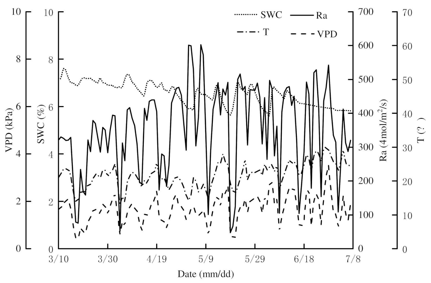
The experiment was conducted from March to July 2018 in a grape greenhouse shed at Yuhe Farm (108°58′ E, 37°49′ N, 961 m above sea level), Yulin city, Shaanxi Province, China. This region has a typical continental marginal monsoon climate. The average annual sunshine duration is 2893.5 h, the average annual temperature is 8.3 °C and the average annual precipitation is 365.7 mm. The soil type in the greenhouse was aeolian sand soil; the soil field capacity (mass) was 0.13 and the soil bulk density was 1.64 g/cm³. Figure 1 shows the daily mean value of meteorological data and soil water content data recorded over the experimental year.

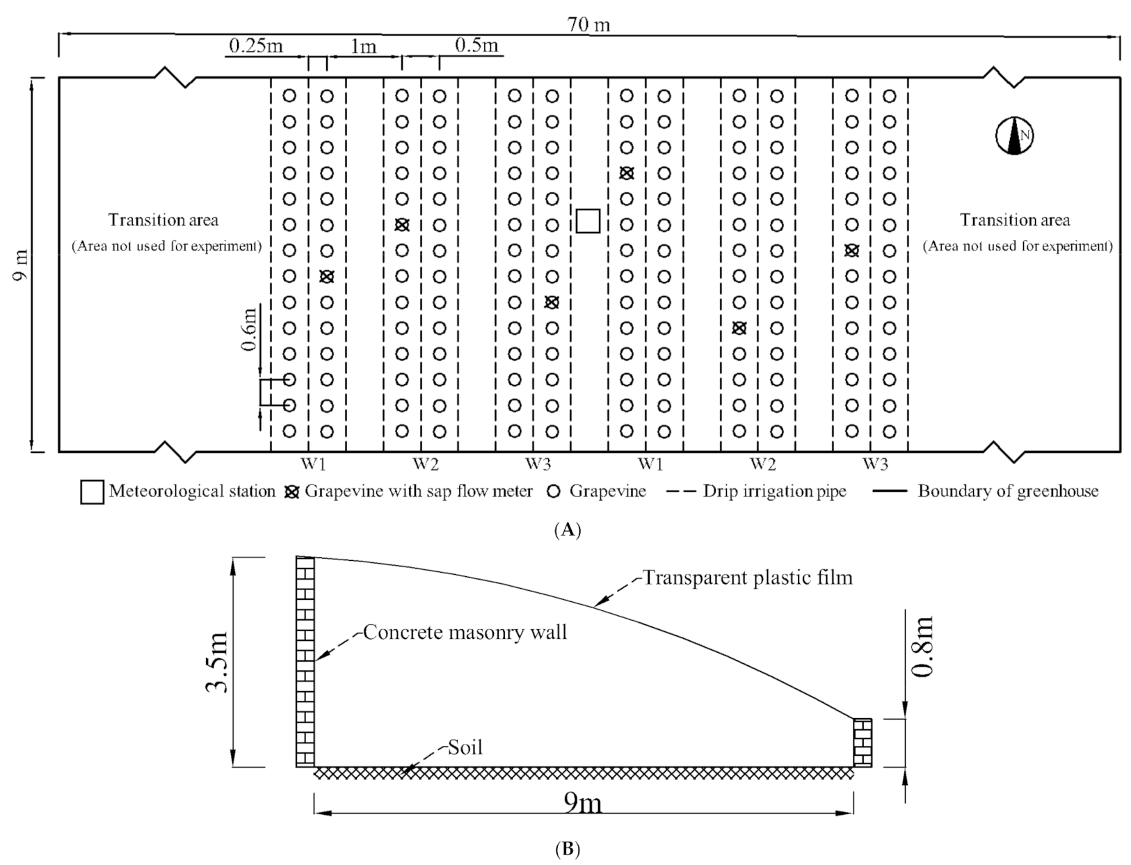
The experimental materials were 5-year-old plants of the early maturing grape variety “6–12”. The length of the greenhouse was 70 m from east to west, and the width of the greenhouse was 9 m from north to south. A planting mode with two kinds of row spacing was adopted. The widths of the large rows and small rows were 1.0 and 0.5 m, respectively. Fourteen grape plants were planted in each row and the plant spacing was 0.6 m. Grape plant growth can be divided into three growth stages: the shoot growth stage (14 March to 26 April), fruit expansion stage (27 April to 3 June) and veraison and maturity stage (4 June 4 to 10 July). Drip irrigation was utilized in the experiment. A drip irrigation pipe was produced by Yangling Qinchuan Water Saving Company, Yangling city, Shaanxi Province, China. The inner diameter of the drip irrigation pipe was 0.02 m; the distance between the drippers was 0.3 m and the design flow of the dripper was 4.0 L/h. The drip irrigation pipe was arranged along the grape planting row, and a drip irrigation pipe was arranged on both sides of each row. The distance between the drip irrigation pipe and the base of the grapevines was 0.25 m. The experimental layout is shown in Figure 2A. The side view of the greenhouse is shown in Figure 2B. The south and top of the greenhouse were constructed of transparent plastic film, and the remainder of the greenhouse was constructed of concrete masonry walls. From 9:00–17:00 on each sunny day, the plastic film on the south side of the greenhouse was uncovered to achieve the purpose of ventilation. The opening height was 1.5 m above the ground. On 11 March 2018, the greenhouse began to be artificially heated. Other agricultural management measures, such as pest control and branch pruning, were carried out according to the local production management mode.

2.2. Experimental Design

Three irrigation treatments, i.e., adequate irrigation (W1, 100% M and M as the irrigation quota), moderate deficit irrigation (W2, 80% M) and deficit irrigation (W3, 60% M), were set up in the experiment. Two replicates were performed for each treatment, for a total of 6 plots. The irrigation amount and irrigation dates are shown in

Table 1. Irrigation amount of grapevine at different growth stages.

Growth Stage	Irrigation Date	Irrigation Amount (m3/ha)
		W1	W2	W3
New shoot growth stage	11 March	293.6	234.5	176.0
	19 March	293.6	234.5	176.0
	27 March	293.6	234.5	176.0
	6 April	293.6	234.5	176.0
	15 April	341.4	273.0	204.0
	25 April	341.4	273.0	204.0
Fruit expansion stage	5 May	341.4	273.0	204.0
	13 May	341.4	273.0	204.0
	20 May	341.4	273.0	204.0
	27 May	341.4	273.0	204.0
Veraison and maturity stage	5 June	293.6	234.5	176.0
	15 June	293.6	234.5	176.0
Total irrigation amount		3810	3045	2280

On the irrigation dates 15 April and 25 April, the grapes flowered, and the plants required a large amount of water, so the irrigation amount was the same as that in the fruit expansion stage.

, and the whole growth period of grapes was irrigated 12 times. Irrigation was applied when the soil moisture content of the W1 treatment reached the lower limit, and all treatments were irrigated simultaneously. M was controlled by establishing upper and lower limits for the soil moisture. The upper limit was the soil field capacity, and the lower limit was 65% of the upper limit during the shoot growth stage and the veraison and maturity stages and 70% of the upper limit during the fruit expansion stage. The calculation formula for M [31] is expressed as follows:

$${\mathrm{M}=1000\mathsf{\gamma }}_{\mathrm{s}}{\mathrm{HP}(\mathsf{\beta }}_1-{\mathsf{\beta }}_2),$$

(1)

where M is the irrigation quota (mm); γ_s is the apparent density, which is numerically equal to the soil bulk density, dimensionless, 1.64; H is the depth of the wet layer (m), 0.5 m; P is the wetness ratio of the drip irrigation, dimensionless, 0.8; β₁ is the upper limit of the soil moisture content (mass) (g/g), which is the soil field capacity, 0.13 and β₂ is the lower limit of the soil moisture content (mass) (g/g), 65% of β₁ at the shoot growth stages and the veraison and maturity stages and 70% of β₁ at the fruit expansion stage.

2.3. Observation Indicators and Methods

2.3.1. Meteorological Data

A WatchDog weather station (Spectrum Technologies Inc., Chicago, IL, USA) was utilized to observe the air temperature (T), relative humidity (RH) and solar radiation (Ra) in the middle of the greenhouse. The instantaneous values of meteorological data were recorded every 30 min. The air vapor pressure deficit (VPD) can be calculated with the following formula [32]:

$$\mathrm{VPD}=0{.6108 \times \mathrm{e}}^{\frac{17.27\mathrm{T}}{\mathrm{T}+237.3}} \times (1-\frac{\mathrm{RH}}{100}),$$

(2)

where VPD is the saturated vapor pressure deficit (kPa); T is the air temperature (°C) and RH is the relative humidity of the air (%).

2.3.2. Soil Water Content (SWC)

An ECH₂O soil moisture sensor (Decision Devices Inc., Pullman, WA, USA) was used to measure the soil volumetric moisture content at a depth range of 0–50 cm below the ground, and sensors were placed every 10 cm in a vertical direction starting from 10 cm soil depth. The recording interval was 30 min, and the soil moisture data measured by the ECH₂O sensor were calibrated by the standard oven-drying method. Before the beginning of the experiment, soil samples were taken every 10 cm with a soil drill until 60 cm, and three days of the soil moisture content was calculated by the oven-drying method. The data recorded by the ECH₂O sensor in different soil layers were recorded. The regression equation was established by a regression analysis between the soil water content calculated by the oven-drying method and the soil water content monitored by ECH₂O. The same method was used to calibrate ECH₂O every 15 days during grape growth. Each plot was fitted with a set of sensors corresponding to the grapevine to which a sap flow meter was fitted. SWC₁₀, SWC₂₀, SWC₃₀, SWC₄₀ and SWC₅₀ represent the soil moisture contents at soil depths of 10, 20, 30, 40 and 50 cm, respectively.

2.3.3. Sap Flow Rate (SF)

During each grape growth stage, two grape plants with a stem diameter of 21–23 mm in good growth conditions were randomly selected from each treatment and equipped with a Flow 32-1K (Dynamax Inc., Troy, MI, USA) wrapped sap flow meter. The sap flow meter was installed at the stem of the grape 30 cm above the ground. The average of the data collected during a 30 min period was automatically recorded by the flow meter every 30 min. The sap flow meter was removed every 6 to 7 days to allow the accumulated heat of the stem to dissipate and to ensure the safety of the probe and normal grape growth. The meter was then reinstalled on the same plant after drying.

2.4. Model Building and Data Analysis

The sap flow rate of the grape plants in each growth stage was selected as the dependent variable. The soil moisture contents at different depths (10, 20, 30, 40 and 50 cm) and the meteorological factors (Ra, T and VPD) were selected as independent variables. Invalid monitoring data obtained during the harvesting period were eliminated (due to the removal of individual sap flow meters or the failure of ECH₂O to display data, the full-day data for these dates were excluded to ensure data synchronization). In this study, the meteorological factors and soil moisture contents at different depths were considered predictive variables, and the sap flow rate was taken as the response variable. Two-thirds of the data were used as the modeling set, and one-third of the data were used as the verification set. The RF algorithm and PLS algorithm were applied in MATLAB R2016a to predict the grape sap flow rate for different irrigation treatments and analyze the relative importance of the predictive variables.

2.4.1. Random Forest Model

RF is a nonlinear, multivariable statistical method. Multiple random samples are obtained through multiple bootstrap sampling, and then corresponding decision-making trees are established based on these samples, thus forming an RF algorithm for classification and regression analysis. For regression problems, the predicted value of the dependent variable is obtained from the average of the results of these decision trees [33]. During the regression simulation of the RF algorithm, two parameters need to be optimized: m_try (number of random variables per decision tree node) and n_tree (number of decision trees generated). In this study, for each iteration, the n_tree value increased from 5 to 500 at intervals of 5 for a total of 100 iterations, and the m_try value increased from 1 to m (m is the number of variables) at intervals of 1 each time for a total of m iterations. The other parameters were set to the default values.

The importance of variables in the RF model is determined by adding random noise to each variable in each decision tree. If the out-of-bag (OOB) error increases, the variable is more important; if the OOB error does not increase, the variable is less important [33]. The calculation method [26] is presented as follows:

$${\mathrm{I}}_{\mathrm{i}}=\frac{\sum {(\mathrm{E}}_{\mathrm{err}002} -{\mathrm{E}}_{\mathrm{err}001})}{{\mathrm{n}}_{\mathrm{tree}}},$$

(3)

where ${\mathrm{I}}_{\mathrm{i}}$ is the importance of variable i, which is a relative value and dimensionless. The larger the value is, the more important the variable is; ${\mathrm{E}}_{\mathrm{err}001}$ is the OOB error and ${\mathrm{E}}_{\mathrm{err}002}$ is the corresponding random OOB error that adds noise interference to variable i in all samples. The OOB error is then recalculated for these circumstances.

2.4.2. Partial Least Squares Model

The PLS model is a novel, multivariate data analysis method. This method is mainly selected for modeling linear regression between multi-predictive variables and multi-response variables. The advantage of PLS is that it can handle datasets with high correlations among predictive variables.

The importance of variables in a PLS model is evaluated by determining the variable importance in the projection (VIP). The ability of the predictive variables to explain the response variables is illustrated by the principal component of the predictive variable synthesis. Assume that there is a response variable y and predictor variables ${\mathrm{x}}_1{,\mathrm{x}}_2\dots {\mathrm{x}}_{\mathrm{k}}$. For the j-th predictor variable, the VIP calculation formula is [28]:

$${\mathrm{VIP}}_{\mathrm{j}}=\sqrt{\frac{\mathrm{k}}{{\sum }_{\mathrm{h}=1}^{\mathrm{m}}{\mathrm{r}}^2\left({\mathrm{y},\mathrm{c}}_{\mathrm{h}}\right)}{\sum }_{\mathrm{h}=1}^{\mathrm{m}}{\mathrm{r}}^2\left({\mathrm{y},\mathrm{c}}_{\mathrm{h}}\right){\mathrm{w}}_{\mathrm{hj}}{}^2},$$

(4)

where VIP_j is the importance of variable j, which is a relative value and dimensionless. The larger the value is, the more important the variable is; k is the number of predictive variables; ${\mathrm{c}}_{\mathrm{h}}$ is the principal component extracted from the predictive variables; $\mathrm{r}\left({\mathrm{y},\mathrm{c}}_{\mathrm{h}}\right)$ is the correlation coefficient between the predictive variables and the principal components and w_hj is the weight of the predictive variable in the principal component.

2.4.3. Uncertainty Analysis

In this study, the d-factor coefficient was used to evaluate the uncertainty of the RF and PLS models. This evaluation was performed by increasing and decreasing the range of 10% for each input item in MATLAB, using the Unifrnd function to generate continuous and evenly distributed random numbers, bringing the newly generated input items into the established model [18] and determining the indicative upper limit (X_U) and lower limit (X_L) with a 95% confidence interval. In addition, the d-factor coefficient was utilized to calculate the average width of the confidence interval, as shown in equations 5 and 6:

$$\mathrm{d}-\mathrm{factor}=\frac{\overline{{\mathrm{d}}_{\mathrm{X}}}}{{\mathsf{\sigma }}_{\mathrm{X}}},$$

(5)

$$\overline{{\mathrm{d}}_{\mathrm{X}}}=\frac{1}{\mathrm{n}}{\sum }_{\mathrm{i}=1}^{\mathrm{n}}\left({\mathrm{X}}_{\mathrm{Ui}}-{\mathrm{X}}_{\mathrm{Li}}\right),$$

(6)

where $\overline{{\mathrm{d}}_{\mathrm{X}}}$ is the average distance between the indicative upper limit (${\mathrm{X}}_{\mathrm{Ui}}$) and the indicative lower limit (${\mathrm{X}}_{\mathrm{Li}}$), that is, the average width of the 95% confidence interval; n is the number of samples and ${\mathsf{\sigma }}_{\mathrm{X}}$ is the standard deviation of the measured sap flow rate. The larger the uncertainty value is, the larger the range of the simulated values near the measured value is, the lower the accuracy of the model is and the more unstable the model is.

2.5. Model Verification

To evaluate the accuracy of the RF and PLS model predictions, the determination coefficient (R²), root mean square error (RMSE, mL/h) and Willmott consistency index (WIA) were selected as evaluation indexes. The calculation formulas are presented as follows:

$${\mathrm{R}}^2=\frac{{\sum }_{\mathrm{i}=1}^{\mathrm{N}}{{(\mathrm{P}}_{\mathrm{i}}-\overline{\mathrm{O}})}^2}{{\sum }_{\mathrm{i}=1}^{\mathrm{N}}{{(\mathrm{O}}_{\mathrm{i}}-\overline{\mathrm{O}})}^2},$$

(7)

$$\mathrm{RMSE}=\sqrt{\frac{{\sum }_{\mathrm{i}=1}^{\mathrm{N}}{\left({\mathrm{O}}_{\mathrm{i}}-{\mathrm{P}}_{\mathrm{i}}\right)}^2}{\mathrm{N}}},$$

(8)

where ${\mathrm{O}}_{\mathrm{i}}$ and ${\mathrm{P}}_{\mathrm{i}}$ are the measured values and predicted values, respectively, of the sap flow rate (mL/h); $\overline{\mathrm{O}}$ is the mean measured value of the sap flow rate (mL/h) and N is the number of samples in the prediction set. When R² and WIA are greater than 0.8, the model is considered to meet the model reliability standard of Jager [34], and the model accuracy is reliable. The dimension of RMSE is the same as that of the simulated value, which facilitates the comparison of different models. The smaller the value is, the smaller the error between the measured value and the value predicted by the model.

3. Results

3.1. Variation in Grape Sap Flow for Different Irrigation Treatments

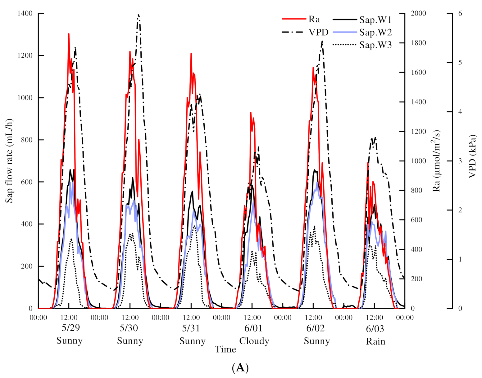
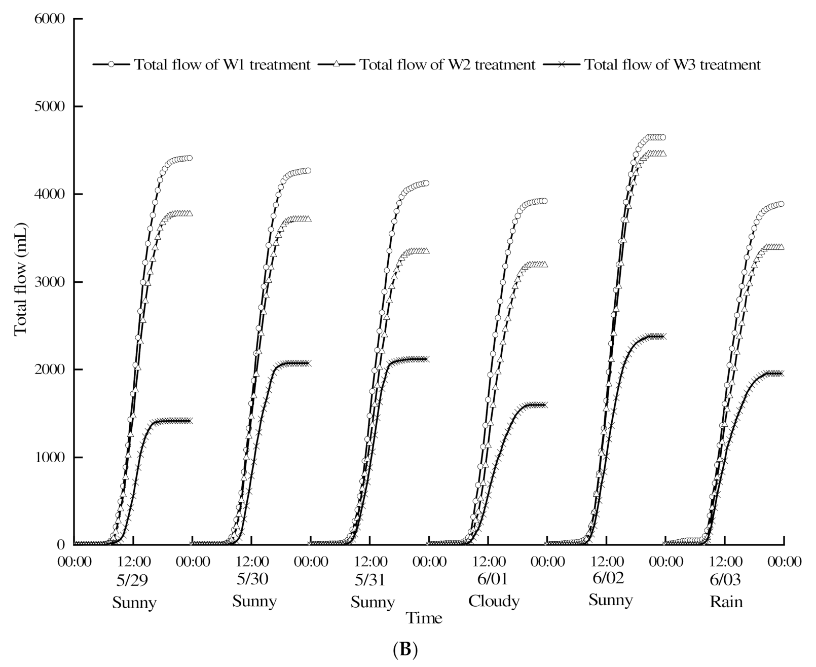
In this study, to accurately explore the influence of different weather and irrigation amounts on the diurnal variation in sap flow, the diurnal variations in the grape sap flow rate for three irrigation treatments and different typical weather conditions were analyzed for six consecutive days from 29 May to 3 June. The irrigation treatments were carried out on 27 May. The effects of the different irrigation treatments on the grape sap flow rate and sap flow are shown in Figure 3. The diurnal variation in the sap flow rate and the changes in Ra and VPD presented unimodal curves. On sunny days, Ra gradually increased in the morning, and the sap flow rate of each treatment began to rise rapidly at approximately 8:00, reached an initial first peak at approximately 11:00, and reached multiple peaks between 11:00 and 16:00. After 16:00, the sap flow rate decreased until it approached zero. The Ra intensity on cloudy and rainy days was lower than that on sunny days, and the peak sap flow rate remained between 200 and 500 mL/h. On sunny days, Ra peaked between 10:00 and 14:00; the sap flow rate peaked between 11:00 and 16:00 and VPD peaked between 12:00 and 17:00. The sap flow rate peaked 1 h later than Ra and 1 h earlier than VPD.

Compared with those in the W1 treatment, the daily mean sap flow rate and daily accumulated sap flow in the W2 treatment were 14.65 lower and 13.92% lower, respectively, while those in the W3 treatment were 46.94 lower and 54.50% lower, respectively. The results showed that the irrigation amount had different degrees of effect on the sap flow rate, and the daily mean sap flow rate and daily accumulated sap flow increased with an increase in the irrigation amount within a certain range.

3.2. Analysis of the Sap Flow Simulation Model

3.2.1. Comparison between Measured Values of Grape Sap Flow and Predicted Values from the Model

The PLS model and RF model were trained with two-thirds of the data from the different input variable sets. After model training, one-third of the detection data were input into the two models for verification. The simulation results from the two models are shown in

Table 2. Analysis of prediction results of different grape sap flow rate models with M-F-S.

Growth Stage	Predictive Variable	Treatment	Omax	RF			PLS
				R2	RMSE	WIA	R2	RMSE	WIA
New shoot growth stage	M-F-S	W1	515.82	0.93	24.75	0.96	0.77	46.77	0.93
		W2	456.12	0.89	26.29	0.97	0.75	40.10	0.93
		W3	195.27	0.85	14.95	0.97	0.80	24.03	0.92
Fruit expansion stage	M-F-S	W1	657.52	0.95	43.54	0.98	0.94	64.23	0.97
		W2	622.49	0.95	39.00	0.98	0.86	60.91	0.96
		W3	406.46	0.93	23.91	0.99	0.88	35.16	0.97
Veraison and maturity stage	M-F-S	W1	562.12	0.93	29.75	0.96	0.80	66.13	0.94
		W2	482.00	0.90	35.51	0.97	0.80	49.26	0.94
		W3	255.98	0.89	24.25	0.97	0.85	28.60	0.96
Whole growth period	M-F-S	W1	808.08	0.95	36.68	0.99	0.79	77.58	0.95
		W2	674.35	0.94	32.22	0.98	0.78	59.73	0.94
		W3	406.46	0.94	20.53	0.98	0.79	36.63	0.94

M-F-S, R², RMSE and WIA represent the meteorological factors and soil moisture content utilized as predictors, the coefficient of determination, the root mean square error (mL/h), and the Willmott index of agreement, respectively; O_max is the maximum measured sap flow rate (mL/h).

and

Table 3. Analysis of prediction results of different grape sap flow rate models by M-F.

Growth Stage	Predictive Variable	Treatment	Omax	RF			PLS
				R2	RMSE	WIA	R2	RMSE	WIA
New shoot growth stage	M-F	W1	515.82	0.85	39.13	0.95	0.77	47.66	0.93
		W2	456.12	0.83	34.69	0.95	0.73	41.93	0.92
		W3	195.27	0.80	17.02	0.93	0.72	24.76	0.92
Fruit expansion stage	M-F	W1	657.52	0.91	54.90	0.97	0.87	68.52	0.96
		W2	622.49	0.90	50.14	0.97	0.84	65.89	0.95
		W3	406.46	0.91	29.27	0.98	0.87	35.76	0.96
Veraison and maturity stage	M-F	W1	562.12	0.84	40.34	0.96	0.74	74.87	0.92
		W2	482.00	0.81	35.35	0.94	0.72	54.41	0.91
		W3	255.98	0.78	23.77	0.95	0.70	33.64	0.94
Whole growth period	M-F	W1	808.08	0.89	46.64	0.96	0.77	84.79	0.93
		W2	674.35	0.85	35.51	0.95	0.76	74.76	0.92
		W3	406.46	0.83	30.85	0.95	0.74	51.91	0.93

M-F, R², RMSE, and WIA represent the meteorological factors applied as predictors, the coefficient of determination, the root mean square error (mL/h) and the Willmott index of agreement, respectively; O_max is the maximum measured sap flow rate (mL/h).

. The results showed that among the different growth stages, the prediction effect of the model during the grape fruit expansion stage was the best, followed by that during the whole growth period, the new shoot growth stage and the veraison and maturity stage. The R² values and the RMSE values of the RF model were 4.79–18.99% higher and 22.64–62.05% lower, respectively, than those of the PLS model. Compared with the PLS model, the simulation results of the RF model were more accurate; the models were tested with the inclusion of only meteorological factors (M-F) as predictors (the prediction results in Table 3), which was slightly less effective than modeling with meteorological factors and soil moisture content (M-F-S) as predictors (the prediction results in Table 2). Compared to the values with M-F as predictors, the R² of the RF model with M-F-S as predictors for the W1, W2 and W3 treatments was 4.40–10.71% higher, 5.56–11.11% higher and 2.20–14.10% higher, respectively, and the RMSE was 20.69–36.75% lower, 0.45–24.21% lower and 2.02–33.45% lower, respectively. Moreover, compared to the values with M-F as predictors, the R² of the PLS model with M-F-S as the predictors for the W1, W2 and W3 treatments were 1.32–8.11% higher, 2.38–11.11% higher and 1.15–21.43% higher, respectively, and the RMSE was 6.26–11.67% lower, 4.36–20.10% lower and 1.68–29.44% lower, respectively. These results confirm that it was helpful to further improve the accuracy of the model predictions of the sap flow rate by considering the soil moisture content as a predictor and that the RF model was more accurate than the PLS model. In addition, as shown in Table 2 and Table 3, as the irrigation amount increases, the prediction performance of the RF model improves, i.e., R² increases. Among the different prediction models, the RF model with M-F-S as the predictors had the best simulation effect during the fruit enlargement stage; the observed values were the closest to the predicted values and the R² and WIA values were greater than 0.8, which conforms to the standard of model reliability in Jager [34].

3.2.2. Comparison between the Measured Value of Grape Sap Flow and the Value Predicted by the Model

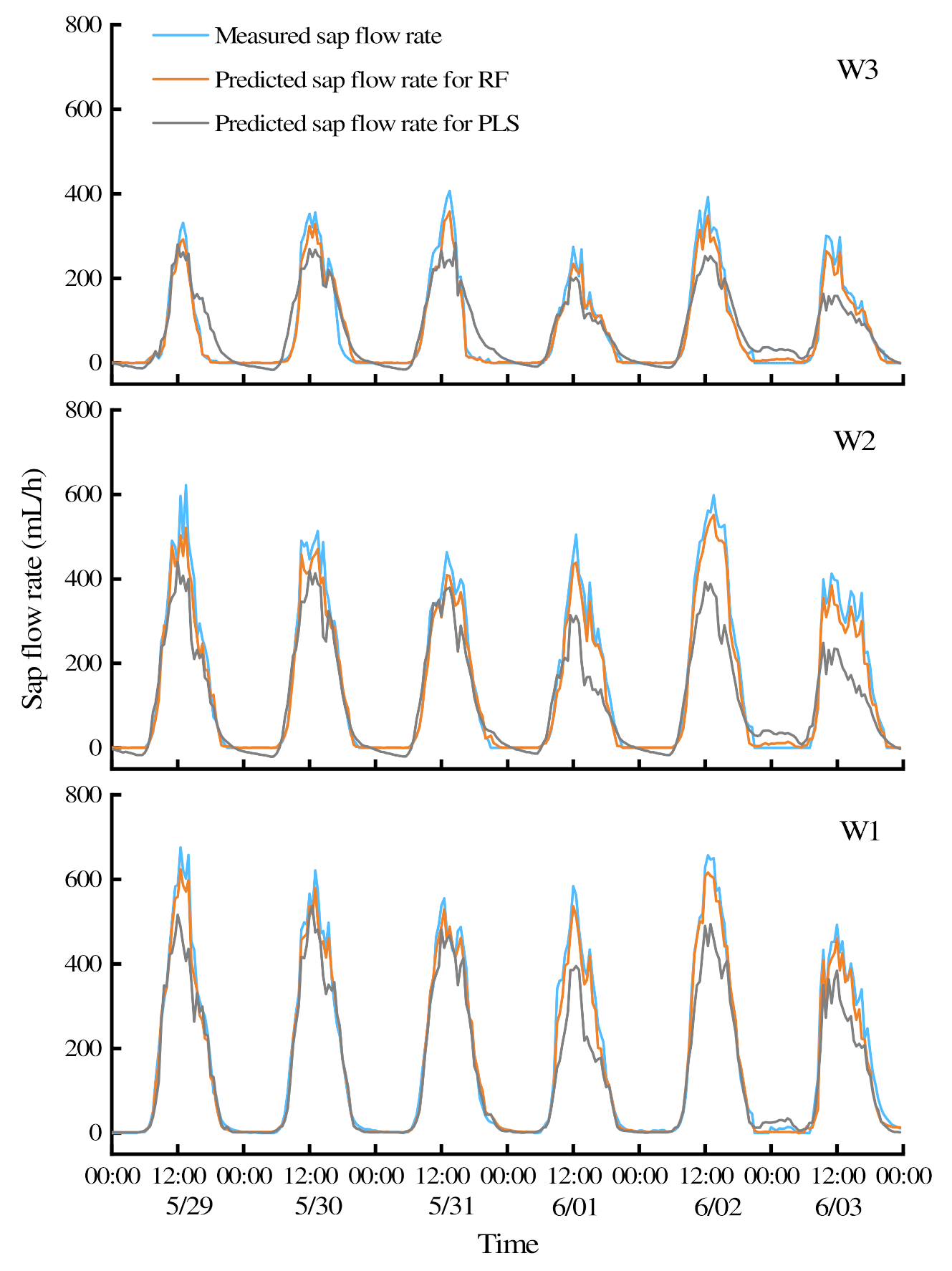
To evaluate the predictive effect of the grape sap flow model, data from the fruit expansion stage were selected, M-F-S was considered as the predictor set, and the RF and PLS models were run to obtain the prediction values. Figure 4 shows the curve of the predicted sap flow values during the fruit expansion stage for the different treatments. The figure shows that the change trends of the predicted sap flow values with W1, W2 and W3 are similar to those of the measured sap flow values. However, the overall forecast value of the model is low and concentrated from 10:00–17:00. During this time period, the error ranges of the RF and PLS models for the W1, W2 and W3 treatments were −37.19–118.04 mL/h and −50.96–230.12 mL/h, −15.93–92.97 mL/h and −17.99–275.50 mL/h, and −59.89–64.90 mL/h and −132.52–176.73 mL/h, respectively. The error variation in the RF model for W1, W2 and W3 during the day was smaller than that of the PLS model; the stability of the RF model was higher; the simulation effect of the RF model was better, and the change in the sap flow rate was better predicted by the RF model than by the PLS model. The RF model simulated the night sap flow rate at close to zero or zero, while the PLS model could not accurately simulate the night sap flow rate and even generated negative values.

3.2.3. Model Uncertainty Analysis

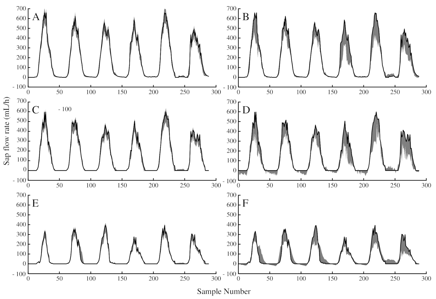
Uncertainty analysis is performed primarily to test whether the predictive effect of a model remains stable after changing an input term and whether the model can still achieve an accurate prediction effect with the new input term. In this study, the model stability was evaluated on the basis of uncertainty analysis and the d-factor value. The d-factor values of the two models in the different grape growth stages are shown in

Table 4. Uncertainty measurement parameter (d-factor) for different models.

Model	Growth Period	d-Factor
		W1	W2	W3	Average Xi	Average
RF	New shoot growth stage	0.40	0.40	0.49	0.43	0.52
	Fruit expansion stage	0.22	0.23	0.25	0.23
	Veraison and maturity stage	0.60	0.48	0.90	0.66
	Whole growth period	0.57	0.48	1.20	0.75
PLS	New shoot growth stage	0.47	0.49	0.54	0.50	0.64
	Fruit expansion stage	0.32	0.42	0.43	0.39
	Veraison and maturity stage	0.74	0.72	0.89	0.78
	Whole growth period	0.72	0.59	1.32	0.88

. Table 4 shows that the average value of the RF model d-factor was low and that the uncertainty of the RF model was lower than that of the PLS model. The uncertainty of the model in different growth stages also varied, and the model uncertainty among stages increased in the following order: fruit expansion stage < new shoot growth stage < whole growth period < veraison and maturity stage. A comparison of the three treatments revealed that the model uncertainty in W3 was higher than that in W2 and W1; the model uncertainty in W1 was lower than that in W2 at the shoot growth and fruit expansion stages and the model uncertainty in W1 was higher than that in W2 at the veraison and maturity stages and for the whole growth period. To better understand the range of variation in the output terms of the two models, the growth stage with the lowest d-factor index, i.e., the fruit expansion stage, was analyzed further, as shown in Figure 5. Of the two models, the RF model exhibited a lesser change in output value caused by the change in input data. The RF model was able to readjust its internal learning mechanism and to adjust the division of each decision tree. In contrast, the output range of the PLS model was large and could not remain stable with the change in input data. To improve the accuracy of the PLS model, we would need to reanalyze the data and adjust the model parameters. In conclusion, the RF model provides higher fitting accuracy and greater stability than the PLS model.

3.3. Evaluation of the Importance of Predictive Variables

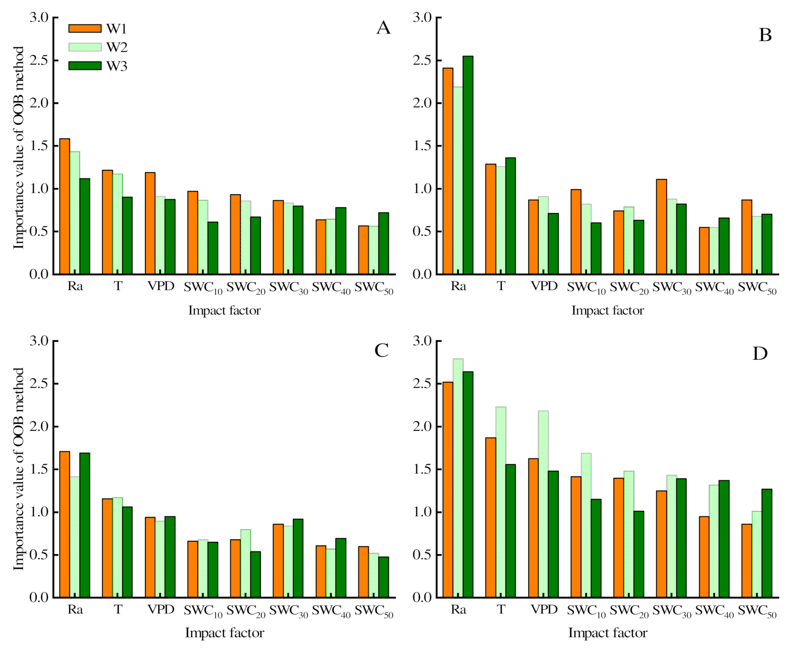
The RF model and PLS model have the ability to evaluate the importance of indicators, and both of them can directly provide a ranking of the importance of all predictors. The RF model and PLS model analyze the relative importance of the predictors based on the OOB method and VIP method, respectively. Figure 6 shows that Ra was the most important variable in the RF sap flow rate prediction model, followed by T and VPD. The order of importance of the water content in different soil layers varied among the different growth stages and different treatments. SWC₃₀ was the most important variable in the W3 treatment at all growth stages. The most important soil moisture layers in the W1 and W2 treatments were generally the three depths of SWC₁₀, SWC₂₀ and SWC₃₀. The OOB value for the RF model indicated the contribution of the predictive variables to the sap flow rate. In the RF model, the importance of meteorological factors accounted for 43.00–57.53%, and the importance of water content in different soil layers accounted for 42.47–57.00%, which indicated that meteorological factors and SWC had an important role in the prediction of the grape sap flow rate by the RF model.

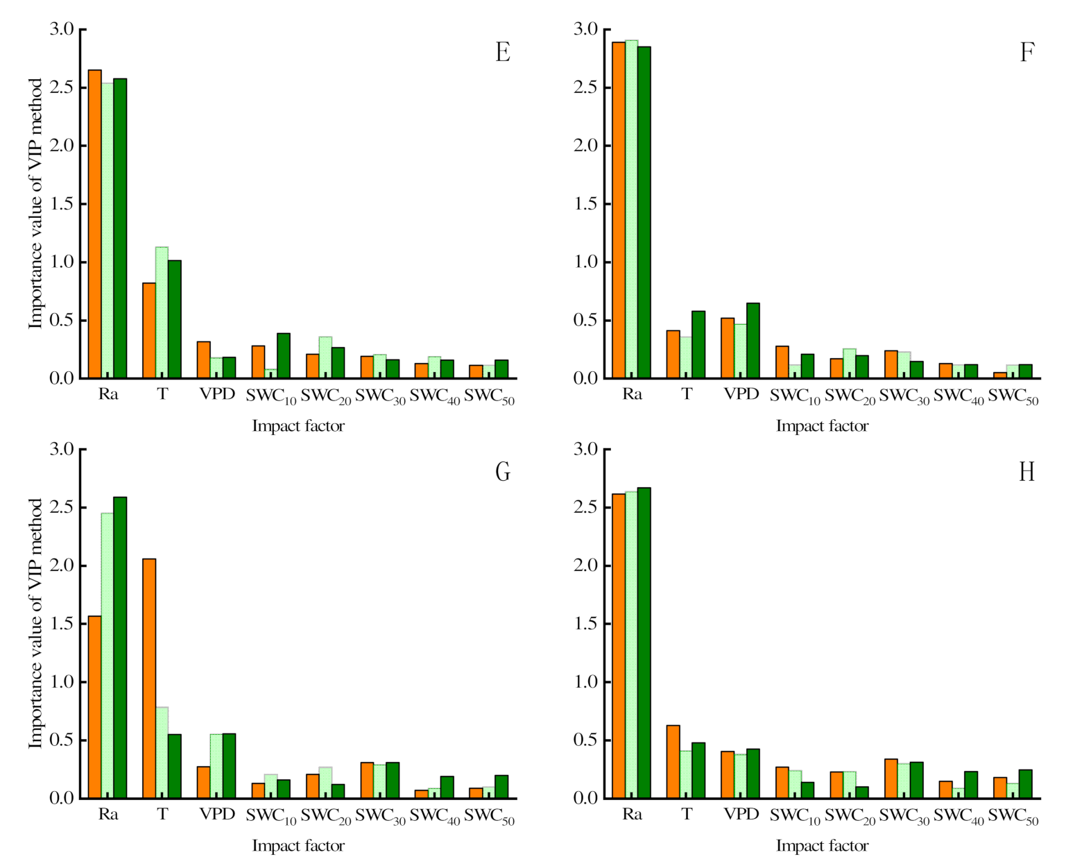
In the PLS prediction model, meteorological factors accounted for 75.76–85.02% of all the prediction variables. In terms of the importance of variables, Ra, T and VPD were the most important factors for predicting the sap flow rate in the PLS model. In conclusion, the importance of different predictive variables to the prediction of the sap flow rate in the RF and PLS models varied. The PLS model reflected the importance of meteorological factors to the sap flow rate but only weakly reflected the importance of soil moisture to the sap flow rate. The RF model reflected the importance of both meteorological factors and different soil moisture layers to the sap flow rate.

4. Discussion

The sap flow measurement method can accurately and continuously provide relevant data of plant water consumption and utilization process without damaging the plant, since numerous studies [5,9,11] have shown that plant transpiration is closely related to sap flow. Both plant physiological and environmental factors comprehensively and interactively impact plant sap flow to various extents. Moreover, their driving mechanisms on sap flow typically change with plant growth status, climate conditions, soil characteristics, management strategies, etc. As a result, sap flow is often estimated using a variety of methods with different forms and complexities, but the estimation performance is far from satisfactory. Regarding further modeling improvement, error source analysis is essential for increasing the model accuracy and stability, leading to further improvement of the accuracy and stability of the sap flow estimation model. This situation placed some limitations on the method of estimating plant water status by estimating sap flow. Therefore, it is important to propose the causes of model error to improve the accuracy of the sap flow estimation model.

In this study, prediction models for the greenhouse grape sap flow rate during different growth stages and for different irrigation treatments were established based on RF and PLS algorithms and achieved satisfactory results. However, the prediction accuracy of the different models varied. The error in the sap flow rate prediction models may have been linked to the following factors:

(1) The verification of the simulation results from the PLS model for sap flow by the test samples revealed that the predicted value at noon and night deviated greatly from the measured value (Figure 4). Figure 3 shows that the sap flow rate showed multiple peaks at noon, which was attributed to the high Ra intensity at noon and the strong atmospheric evaporation capacity in the greenhouse. To avoid excessive water loss from the grape plants, the stomata of the grape leaves were regulated and the phenomenon of “midday depression” appeared [35,36]. In addition, the variation trends of meteorological factors and the sap flow rate are quite different at night and during the day and the values of Ra and the sap flow rate at night are effectively zero (Figure 3). According to the evaluation and analysis of the importance of variables, the PLS model gave the most weight to meteorological factors when predicting the sap flow rate in this study (Figure 6). When external factors change, such as the “midday depression” phenomenon in plants, and Ra exhibits great variation between daytime and nighttime, the parameters of the PLS model cannot be adjusted in time to reflect the changes in meteorological factors, making it unable to accurately simulate the sap flow rate. This disadvantage results in model simulation error.

In the process of constructing the RF model, some features are randomly selected from the sample set, and the optimal hyperplane (i.e., established decision tree) is implemented for this subset. This randomness increases the deviation in the RF model, but the RF is the average result of each decision tree in the regression problem, which compensates for the increase in deviation. Therefore, under different test conditions, with enough training data, the RF algorithm can carry out the optimal hyperplane with new data and quickly complete the data analysis and modeling. Unlike the PLS model, the RF model avoids the problem of the parameters of the traditional linear model not being transferred and is thus able to fully reflect the influence of meteorological factors and soil moisture on the sap flow rate.

(2) In this study, differences in the variation in the grape sap flow rate under different irrigation conditions were observed. According to Table 2 and Table 3, the simulation accuracy of the RF model trained by sample data for the three treatments improved, but in general, the simulation results were more reliable in the stage with the most abundant water conditions (the R² was higher and the error was smaller). This phenomenon was more obvious when M-F was the predictive variable than when M-F-S were the predictive variables; this result indicates that soil water can indirectly reflect the effect of water deficit on plant water consumption to a certain extent, but cannot fully reflect the effect of water deficit on plant water consumption. Therefore, in follow-up simulation improvement studies, we can consider adding several indexes of the plant itself (such as the stem water potential, leaf water potential and abscisic acid concentration) as predictive variables in the simulation process to fully express the effect of drought on the transpiration dynamics of plants.

(3) The prediction accuracy of the model in the different grape growth stages differed. The prediction effect in the fruit expansion stage was the best, followed by that in the new shoot growth stage and the veraison and maturity stage. These differences may have occurred because the size of the canopy is an important factor affecting sap flow in grape plants [37]; however, the relevant indicators of canopy size were not considered in the prediction variables in this study. During the new shoot growth stage, new branches grow, new leaves proliferate and the leaf area gradually increases. After the fruit expansion stage, the leaf area of the plant reaches a maximum and tends to stabilize. In subsequent veraison and maturity stages, the leaves gradually turn yellow and fall off, and the effective leaf area for transpiration begins to decrease. During the growth stages with large, dynamic changes in leaf area, a close relationship between canopy characteristics and sap flow exists. Therefore, leaf area or related indicators should be considered variables in the process of establishing a sap flow prediction model to improve the prediction accuracy. When leaf area growth reached a relatively stable stage, the leaf area/leaf area index was not the main factor controlling sap flow, and the change in sap flow was affected mainly by environmental factors [38,39]. During this stage, the effect of leaf area-related indexes on the sap flow prediction results was relatively small.

In this paper, an estimation model for greenhouse grape sap flow was established based on the RF algorithm; the model was evaluated by uncertainty analysis and good prediction results were obtained. However, predictions of sap flow in different crops and under different experimental conditions need further verification. The main meteorological factors affecting sap flow in greenhouses are Ra, T and RH [26]; in contrast, the external factors in the field are complex and changeable, and it becomes necessary to consider the additional impacts of rainfall and wind speed. The distribution of soil moisture in the field is affected mainly by rainfall. During rainfall, the soil moisture content in shallow soils increases rapidly; it decreases rapidly after the rainfall ends. The increase in deep soil moisture lags behind the occurrence of rainfall. The water content in different soil layers fluctuates greatly, which may affect the accuracy of stemflow prediction models. The amount and timing of rainfall also affect the soil moisture content, so the simulation accuracy and practical application of sap flow models need to be further verified in future studies.

5. Conclusions

This study showed that the sap flow rate of grapes for different irrigation treatments and at different growth stages in greenhouses could be better predicted by the RF model than by the PLS model and that the prediction accuracy during the fruit expansion stage was the highest. Compared with those of the PLS model, the R² of the RF model was 4.79–18.99% higher and the RMSE was 22.64–62.05% lower; the WIA of the RF model was greater than 0.9. The model uncertainty analysis revealed that the uncertainty in the W3 treatment was higher than those in the W2 and W1 treatments. The average value of the d-factor of the PLS model was larger than that of the RF model, and the output range of the RF model was smaller, so the model was more stable. Including data on the moisture content of different soil layers in the model as a predictor in combination with meteorological factors improved the prediction accuracies of the two models. The contributions of the different predictors to the establishment of the two sap flow rate models differed. Meteorological factors and the water content of different soil layers were equally important in the RF model, while the most important variables in the PLS model were mainly meteorological factors.

References

- Martin, J.; Markus, R.; Philippe, C.; Sonia, I.S.; Justin, S.; L, G.M.; Gordon, B.; Alessandro, C.; Jiquan, C.; Richard, d.J.; et al. Recent decline in the global land evapotranspiration trend due to limited moisture supply. Nature 2010, 467, 951–954. [Google Scholar] [CrossRef]
- Trenberth, K.E.; Fasullo, J.T.; Kiehl, J. Earth’s Global Energy Budget. Bull. Am. Meteorol. Soc. 2009, 90, 311–323. [Google Scholar] [CrossRef]
- Scott, J.; Sharp, Z.D.; Gibson, J.J.; Jean, B.S.; Yi, Y.; Fawcett, P.J. Terrestrial water fluxes dominated by transpiration. Nature 2013, 496, 347–350. [Google Scholar]
- Lagergren, F.; Lindroth, A. Transpiration response to soil moisture in pine and spruce trees in Sweden. Agric. For. Meteorol. 2002, 112, 67–85. [Google Scholar] [CrossRef]
- Myburgh, P.A. Estimating Transpiration of Whole Grapevines under Field Conditions. South Afr. J. Enol. Vitic. 2016, 37, 47–60. [Google Scholar] [CrossRef]
- Fernández, J.; Moreno, F.; Martín-Palomo, M.; Cuevas, M.V.; Torres-Ruiz, J.M.; Moriana, A. Combining sap flow and trunk diameter measurements to assess water needs in mature olive orchards. Environ. Exp. Bot. 2011, 72, 330–338. [Google Scholar] [CrossRef]
- Zhang, Y.; Kang, S.; Ward, E.J.; Ding, R.; Xin, Z.; Rui, Z. Evapotranspiration components determined by sap flow and microlysimetry techniques of a vineyard in northwest China: Dynamics and influential factors. Agric. Water Manag. 2011, 98, 1207–1214. [Google Scholar] [CrossRef]
- Chen, D.; Wang, Y.; Liu, S.; Wei, X.; Wang, X. Response of relative sap flow to meteorological factors under different soil moisture conditions in rainfed jujube (Ziziphus jujuba Mill.) plantations in semiarid Northwest China. Agric. Water Manag. 2014, 136, 23–33. [Google Scholar] [CrossRef]
- Chen, R.; Kang, E.; Zhao, W.; Zhang, Z.; Zhang, J. Trees transpiration response to meteorological variables in arid regions of Northwest China. Acta Ecol. Sin. 2004, 24, 477–485. [Google Scholar]
- Novak, V.; Hurtalova, T.; Matejka, F. Predicting the effects of soil water content and soil water potential on transpiration of maize. Agric. Water Manag. 2005, 76, 211–223. [Google Scholar] [CrossRef]
- Zhang, B.; Xu, D.; Liu, Y.; Li, F.; Cai, J.; Du, L. Multi-scale evapotranspiration of summer maize and the controlling meteorological factors in north China. Agric. For. Meteorol. 2016, 216, 1–12. [Google Scholar] [CrossRef]
- Nicolas, E.; Torrecillas, A.; Ortu?O, M.F.; Domingo, R.; Alarcón, J. Evaluation of transpiration in adult apricot trees from sap flow measurements. Agric. Water Manag. 2005, 72, 131–145. [Google Scholar] [CrossRef]
- Tognetti, R.; D’Andria, R.; Morelli, G.; Alvino, A. The effect of deficit irrigation on seasonal variations of plant water use in Olea europaea L. Plant Soil 2005, 273, 139–155. [Google Scholar] [CrossRef]
- Traore, S.; Wang, Y.M.; Kerh, T. Artificial neural network for modeling reference evapotranspiration complex process in Sudano-Sahelian zone. Agric. Water Manag. 2010, 97, 707–714. [Google Scholar] [CrossRef]
- Tabari, H.; Kisi, O.; Ezani, A.; Talaee, P.H. SVM, ANFIS, regression and climate based models for reference evapotranspiration modeling using limited climatic data in a semi-arid highland environment. J. Hydrol. 2012, 444–445, 78–89. [Google Scholar] [CrossRef]
- Deo, R.C.; Ahin, M. Application of the extreme learning machine algorithm for the prediction of monthly Effective Drought Index in eastern Australia. Atmos. Res. 2015, 153, 512–525. [Google Scholar] [CrossRef] [Green Version]
- Liu, X.; Kang, S.; Li, F. Simulation of artificial neural network model for trunk sap flow of Pyrus pyrifolia and its comparison with multiple-linear regression—ScienceDirect. Agric. Water Manag. 2009, 96, 939–945. [Google Scholar] [CrossRef]
- Du, B.; Hu, X.; Wang, W.; Ma, L.; Zhou, S. Stem flow influencing factors sensitivity analysis and stem flow model applicability in filling stage of alternate furrow irrigated maize. Sci. Agric. Sin. 2018, 51, 233–245. [Google Scholar]
- Fan, J.; Zheng, J.; Wu, L.; Zhang, F. Estimation of daily maize transpiration using support vector machines, extreme gradient boosting, artificial and deep neural networks models. Agric. Water Manag. 2021, 245, 106547. [Google Scholar] [CrossRef]
- Kumar, M.; Raghuwanshi, N.S.; Singh, R. Artificial neural networks approach in evapotranspiration modeling: A review. Irrig. Ence 2011, 29, 11–25. [Google Scholar] [CrossRef]
- Huang, G.B.; Zhu, Q.Y.; Siew, C.K. Extreme learning machine: Theory and applications. Neurocomputing 2006, 70, 489–501. [Google Scholar] [CrossRef]
- Wang, Z.; Lai, C.; Chen, X.; Yang, B.; Zhao, S.; Bai, X. Flood hazard risk assessment model based on random forest. J. Hydrol. 2015, 527, 1130–1141. [Google Scholar] [CrossRef]
- Rodriguez, G.V.; Mendes, M.P.; Garcia, S.M.J.; Chica, O.M.; Ribeiro, L. Predictive modeling of groundwater nitrate pollution using Random Forest and multisource variables related to intrinsic and specific vulnerability: A case study in an agricultural setting (Southern Spain). Sci. Total. Environ. 2014, 476-477, 189–206. [Google Scholar] [CrossRef] [PubMed]
- Gong, H.; Sun, Y.; Shu, X.; Huang, B. Use of random forests regression for predicting IRI of asphalt pavements. Constr. Build. Mater. 2018, 189, 890–897. [Google Scholar] [CrossRef]
- Longjun, D.; Xibing, L.I.; Peng, K. Prediction of rockburst classification using Random Forest. Trans. Nonferrous Met. Soc. China 2013, 23, 472–477. [Google Scholar]
- Wu, M.; Feng, Q.; Wen, X.; Deo, R.C.; Sheng, D. Random forest predictive model with uncertainty analysis capability for estimation of evapotranspiration in an arid oasis region. Hydrol. Res. 2020, 51, 648–665. [Google Scholar] [CrossRef]
- Fukuda, S.; Spreer, W.; Yasunaga, E.; Yuge, K.; Sardsud, V.; Müller, J. Random Forests modelling for the estimation of mango (Mangifera indica L. cv. Chok Anan) fruit yields under different irrigation regimes. Agric. Water Manag. 2013, 116, 142–150. [Google Scholar] [CrossRef]
- Oussama, A.; Elabadi, F.; Platikanov, S.; Kzaiber, F.; Tauler, R. Detection of Olive Oil Adulteration Using FT-IR Spectroscopy and PLS with Variable Importance of Projection (VIP) Scores. J. Am. Oil Chem. Soc. 2012, 89, 1807–1812. [Google Scholar] [CrossRef]
- Ming, Z.; Mu, H.; Gang, L.; Ning, Y. Forecasting the transport energy demand based on PLSR method in China. Energy 2009, 34, 1396–1400. [Google Scholar]
- Shrestha, D.L.; Kayastha, N.; Solomatine, D.P. A novel approach to parameter uncertainty analysis of hydrological models using neural networks. Hydrol. Earth Syst. Sci. Discuss. 2009, 6, 1235–1248. [Google Scholar] [CrossRef] [Green Version]
- Ru, C.; Hu, X.; Wang, W.; Ran, H.; Song, T.; Yinyin, G. Evaluation of the Crop Water Stress Index as an Indicator for the Diagnosis of Grapevine Water Deficiency in Greenhouses. Horticulturae 2020, 6, 86. [Google Scholar] [CrossRef]
- Allen, R.; Pereira, L.; Raes, D.; Smith, M.; Allen, R.G.; Pereira, L.S.; Martin, S. Crop Evapotranspiration: Guidelines for Computing Crop Water Requirements, FAO Irrigation and Drainage Paper 56. FAO 1998, 56, D05109. [Google Scholar]
- Breiman, L. Random forests. Mach. Learing 2001, 45, 5–32. [Google Scholar] [CrossRef] [Green Version]
- Jager, J.M.D. Accuracy of vegetation evaporation ratio formulae for estimating final wheat yield. Ieice Trans. Fundam. Electron. Commun. Comput. Sci. 1994, 71, 1480–1486. [Google Scholar]
- Demrati, H.; Boulard, T.; Fatnassi, H.; Bekkaoui, A.; Majdoubi, H.; Elattir, H.; Bouirden, L. Microclimate and transpiration of a greenhouse banana crop. Biosyst. Eng. 2007, 98, 66–78. [Google Scholar] [CrossRef]
- Qiu, R.; Kang, S.; Li, F.; Du, T.; Tong, L.; Wang, F.; Chen, R.; Liu, J.; Li, S. Energy partitioning and evapotranspiration of hot pepper grown in greenhouse with furrow and drip irrigation methods. Sci. Hortic. 2011, 129, 790–797. [Google Scholar] [CrossRef]
- Malheiro, A.C.; Pires, M.; Conceio, N.; Claro, A.M.; Moutinho-Pereira, J. Linking Sap Flow and Trunk Diameter Measurements to Assess Water Dynamics of Touriga-Nacional Grapevines Trained in Cordon and Guyot Systems. Agriculture 2020, 10, 315. [Google Scholar] [CrossRef]
- Tie, Q.; Hu, H.; Tian, F.; Guan, H.; Lin, H. Environmental and physiological controls on sap flow in a subhumid mountainous catchment in North China. Agric. For. Meteorol. 2017, 240, 46–57. [Google Scholar] [CrossRef]
- Chunwei, L.; Taisheng, D.; Fusheng, L.; Shaozhong, K.; Sien, L.; Ling, T. Trunk sap flow characteristics during two growth stages of apple tree and its relationships with affecting factors in an arid region of northwest China. Agric. Water Manag. 2012, 104, 193–202. [Google Scholar] [CrossRef]
Figure 1.
Daily mean values of meteorological data (Ra, T and VPD represent solar radiation, air temperature and air vapor pressure deficit, respectively) and soil water content data (SWC represents soil water content measured by the ECH2O sensor in different treatments and different soil layers) during the growing season.
Figure 2.
(A) A schematic drawing of the plant distribution in the greenhouse; (B) the side view of the greenhouse.
Figure 3.
(A) Diurnal variation in sap flow rate (Sap.W1, Sap.W2 and Sap.W3 represents an average of measurements of sap flow rate from two grape trees of W1, W2 and W3 treatments, respectively), Ra (solar radiation) and VPD (vapor pressure deficit); (B) sap flow accumulation curve in different irrigation treatments.
Figure 4.
Comparison of trends in simulated and measured values during the fruit expansion stage.
Figure 5.
(A) The uncertainty analysis for the RF model in the W1 treatment during the fruit expansion stage; (B) uncertainty analysis for the PLS model in the W1 treatment during the fruit expansion stage; (C) uncertainty analysis for the RF model in the W2 treatment during the fruit expansion stage; (D) uncertainty analysis for the PLS model in the W2 treatment during the fruit expansion stage; (E) the uncertainty analysis for the RF model in the W3 treatment during the fruit expansion stage; (F) uncertainty analysis for the PLS model in the W3 treatment during the fruit expansion stage. The black solid line is the measured sap flow value; the shaded area is the 95% confidence interval.
Figure 6.
(A) Importance of predictor variables in the RF model during the shoot growth stage; (B) importance of predictor variables in the RF model during the fruit expansion stage; (C) importance of predictor variables in the RF model during the veraison and maturity stage; (D) importance of predictor variables in the RF model during the whole growth period; (E) importance of predictor variables in the PLS model during the shoot growth stage; (F) importance of predictor variables in the PLS model during the fruit expansion stage; (G) importance of predictor variables in the PLS model during the veraison and maturity stage; (H) importance of predictor variables in the PLS model during the whole growth period. Ra, T and VPD represent solar radiation, air temperature and air vapor pressure deficit, respectively; SWC10, SWC20, SWC30, SWC40 and SWC50 represent the soil moisture contents at soil depths of 10, 20, 30, 40 and 50 cm, respectively.