Article

Probability of Non-Exceedance of Arsenic Concentration in Groundwater Estimated Using Stochastic Multicomponent Reactive Transport Modeling

1
Autorità di Bacino Distrettuale delle Alpi Orientali, Cannaregio 4314, 30121 Venice, Italy
2
Dipartimento di Scienze della Terra “A. Desio”, Università degli Studi di Milano (UNIMI), Via Mangiagalli 34, 20133 Milan, Italy
3
Department of Geology, Institute of Geography and Earth Sciences, Eötvös Loránd University, Pázmány P. stny. 1/c, 1117 Budapest, Hungary
4
Department of Geosciences, Università degli Studi di Padova, Via Gradenigo 6, 35131 Padova, Italy
*
Author to whom correspondence should be addressed.
Water 2021, 13(21), 3086; https://doi.org/10.3390/w13213086
Submission received: 10 September 2021 / Revised: 26 October 2021 / Accepted: 31 October 2021 / Published: 3 November 2021

Abstract

:
Stochastic multicomponent reactive transport modeling is a powerful approach to quantify the probability of non-exceedance (PNE) of arsenic (As) critical concentration thresholds in groundwater. The approach is applied to a well-characterized shallow alluvial aquifer near Venice, Italy. Here, As mobility depends primarily on rainfall-controlled redox-dependent precipitation-dissolution of iron hydroxides. A Monte-Carlo analysis based on a calibrated three-dimensional flow and transport model targeted the geochemical initial conditions as the main source of uncertainty of As concentrations in the studied aquifer. It was found that, during 115 simulated days, the fraction of the entire aquifer volume with As > 10 μgL−1 decreased on average from ~43% to ~39% and the average As concentration from ~32 μgL−1 to ~27 μgL−1. Meanwhile, PNE increased from 55% to 60% when 10 μgL−1 was set as target threshold, and from 71% to 78% for 50 μgL−1. The time dependence of As attenuation can be ascribed to the increase of oxidizing conditions during rainfall-dependent aquifer recharge, which causes As sorption on precipitating iron hydroxides. When computing the same statistics for the shallowest 6 m, As attenuation was even more evident. The volume fraction of aquifer with As > 10μgL−1 dropped from 40% to 28% and the average As concentration from 31 μgL−1 to 20 μgL−1, whereas PNE increased from 58% to 70% for As < 10 μgL−1 and from 71% to 86% for As < 50 μgL−1. Thus, the wells screen depth in the aquifer can be a critical aspect when estimating As risk, owing to the depth-dependent relative change in redox conditions during rainfall events.

1. Introduction

Geogenic aquifer contamination by arsenic (As) is a common issue in several countries of the world [1,2,3]. An intake of high As concentrations can cause critical diseases such as skin lesions, ulcers or cancer. The World Health Organization (WHO) recommends As concentration in drinking water not to exceed a threshold of 10 μgL−1 (i.e., 10 ppb) [4]. However, up to 220 million people may be potentially exposed to As > 10 μgL−1 [3], the vast majority being in Asia, where groundwater in contact with shallow (<50 m), commonly Holocene sediments can exceed the WHO threshold by a factor of 100 [5]. In many countries, the As concentration threshold for drinking is set to 50 μgL−1 [6]. Yet, a lifetime exposure to just 50 μgL−1 of As in drinking water may kill one in a hundred people prematurely [7].
Most groundwater consumers are unaware of As-related health risks. In alluvial aquifers, shallow private tube wells, sometimes reaching just a few meters below the ground surface, can be easily drilled and ignored by authorities. Therefore, mapping the spatial and temporal (i.e., spatiotemporal) variations of elevated As concentrations in groundwater is of the uttermost urgence for public administrations and regulators. In the European Union, monitoring of groundwater health has been a mandatory task for local administrations since the 2000s, according to the Water Framework Directive (2000/60/EC) and the Groundwater Directive (2006/118/EC).
Reactive transport modeling has been increasingly adopted in recent years to assist decision makers to quantify the potential extension of As contamination in aquifers [8,9]. Specifically, multicomponent reactive transport modeling (MRTM) has been deployed as a tool that enables elucidating and simulating the controls of As mobility in aquifers and predicting its concentrations in space and time [10,11,12,13,14]. These models can mechanistically simulate the effects of As-bearing rocks or sediments, which are naturally found in aquifers.
The development of predictive MRTM to estimate the spatiotemporal variability of biogeochemical reactive species in aquifers remains a complicated task. A key reason is that aquifers are texturally and compositionally heterogeneous across multiple scales. This makes the complete mapping of model parameters incomplete, rendering the predictive model outputs epistemically uncertain [15]. Although averaging (i.e., homogenizing) aquifer parameters is a common practice among modelers, embedding parameter heterogeneities remains fundamental to properly mimic the transport dynamics of reactive dissolved species, such as As [16,17], particularly when performing risk assessment.
When making model-based predictions under uncertainty, stochastic modeling is widely used in hydrogeology to circumvent the limitations of deterministic modeling [18,19,20]. In stochastic analysis, model input parameters are treated as random spatial functions, whereas the model outputs are expressed in terms of probability density functions. Statistical indicators derived from these functions are used as metrics to quantify one or more desired target variables (e.g., the concentration of a polluting aqueous species) [18].
Stochastic MRTM are useful tools that can be used to estimate the probability of non-exceedance (PNE) of an aquifer toxic compound under uncertainty [21]. Quantifying PNE according to different concentration thresholds is a key input for As risk assessment [22,23]. Nonetheless, stochastic reactive transport modeling has been only occasionally applied to the analysis of As transport [24]. We have no knowledge of stochastic MRTM targeting regional scale As mobility in heterogeneous aquifers, as addressed in the present work.
The epistemic uncertainty related to the incomplete mapping of the geochemical initial conditions (GICs) represents a crucial limitation for the reliability of the MRTM predictions. When a system is far from chemical equilibrium, its initial geochemical status is perturbed with time as the flow, transport and geochemical transformations occur. Setting the correct GICs at each model cell is fundamental to properly compute the PNE of a desired toxic compound. Unfortunately, GICs are typically measured at a few locations (i.e., the boreholes in which geochemical analyses were performed) and repeated at time intervals which may exceed the frequency at which contaminants concentrations oscillate and temporarily exceed the regulatory limits. The resulting epistemic uncertainty of the GICs translates into uncertainty in the model outputs. In statistical analysis, the problem is known as error propagation or propagation of uncertainty. In fluid dynamics, error propagation as a function of the uncertain initial conditions has been addressed since the 1960s [25]. However, our literature review revealed that uncertainty in GICs has not been yet widely explored for MRTM-based forecasts, especially for As-related problems.
In this work, we developed a new Monte-Carlo-based stochastic analysis based on three-dimensional (3-D) MRTM. The model, never presented before, was used to compute the time dependent PNE of As concentrations in the shallow Holocene aquifers of the Western Agricultural Areas (WAA). This site is a well-characterized subset of the Venetian Alluvial Plain in Northern Italy (Figure 1). Previous works on the area [26,27,28,29] have generally concluded that As concentrations can be considered a random spatiotemporal variable, amenable to be modelled using probabilistic and geostatistical analysis. This makes the WAA an appealing case study to evaluate the actual usefulness of the stochastic model to predict the PNE of arsenic concentrations above the 10 μgL−1 and 50 μgL−1 critical thresholds.
Our primary goal is to demonstrate the use of a stochastic multicomponent reactive transport model to assess the probability of As non-exceedance, treating the geochemical initial conditions of the MRTMs as the main stochastic parameter. Indeed, for this study a limited and incomplete amount of geochemical data is available to parametrize the initial condition of the MRTMs. More broadly, we aim to showcase the benefit of stochastic MRTM as a decisional tool for administrations and regulators when dealing with complex hydrogeological systems at regional scales. Although our study targets a specific contaminant in a specific aquifer, the developed methodology is general and can be applied to virtually any kind of aquifer and toxic compound.

2. Materials and Methods

2.1. Background

The Venetian Alluvial Plain (VAP) is a multilevel stratified aquifer underlying the Drainage Basin of Venice Lagoon (in Italian, “Bacino Scolante della Laguna di Venezia”) (Figure 1a). This densely populated region near Venice (Italy) is composed of 108 municipalities, covering an area of about 2000 km2 and with a population close to 1 million inhabitants (Italian National Institute of Statistics, 2001). Arsenic concentrations in the VAP shallow groundwater can exceed the Italian maximum concentration limit and the WHO-recommended threshold of 10 μgL−1 [26,27,28,29]. Following the EU Water and Groundwater Directive, implemented in Italy mainly through the National Decree D.Lgs 152/2006, an excess of As concentration in groundwater implies that local administration should properly monitor and characterize the extension of the contamination, the natural background levels and thresholds values that can potentially entail a risk for the groundwater consumers. Although the water distribution is supplied to virtually all households in the Drainage Basin of Venice Lagoon, groundwater is mainly used for irrigation purposes and there could be a potential for direct human consumption through private wells.
The controls of elevated As concentrations in the VAP have remained unknown for years. Hot spots of dissolved As in groundwater, sometimes exceeding 200 μgL−1, are variably distributed in the shallow VAP aquifer, without an apparent relationship with high concentrations of As-bearing minerals [26]. Moreover, concentrations measured at a few piezometers were found to fluctuate with time above or below the 10 μgL−1 concentration thresholds. This observation was described during different surveys [26], including the 2009 and 2017 surveys reported in Supplementary Information (Section SI-1) and later analyzed in this work. The erratic occurrence of As excess in groundwater urged environmental regulators to perform systematic analyses and establish collaborations with universities and other research centers to unravel the factors controlling As mobility in the VAP. A target of these activities was to quantify the probability of non-exceedance (PNE) of As concentrations above 10 μgL−1, to be later used for measuring the risk to which the population could be exposed if As-contaminated groundwater is consumed unwarily.
In a recent study, Dalla Libera et al. [29] (hereafter, “DL2020”) proposed a conceptual model that mechanistically explains the spatiotemporal As variations in the VAP aquifer. The study focused on the Western Agricultural Areas (WAA), a well characterized area of the distal portion of the VAP towards the Adriatic Sea. According to DL2020, the aquifer is stratified and composed of multiple sandy layers embedded into a fine-grained matrix (Figure 1b). Between 6 December 2017 and 26 March 2018 (i.e., over 115 days), weekly geochemical measurements and continuous groundwater head logs were collected from three fully penetrating observation wells (piezometers PZP36, PZP40 and PZP41). The piezometers are drilled to an average depth of about 10 m from the ground surface.
DL2020 found that rainfall events were well correlated to the decrease of concentrations of aqueous As and Fe and to the increase of oxidizing-reducing potential (ORP). The shift towards higher ORP values and associated attenuation of As and Fe as a consequence of rainfall events was more evident when a limited thickness (<1 m) of fine-grained sediments was observed above the sandy aquifer, according to the boreholes’ stratigraphic logs. When such fine-grained sediments were thicker, the ORP positive shift was more limited, and no significant variations of As and Fe were observed.
Based on these observations, DL2020 hypothesized that rainfall-driven redox-controlled precipitation and dissolution of ferric hydroxides (HFOs) is a main control of As in the shallow VAP aquifers. Similar to the conceptual model proposed for other alluvial aquifers of the world [1,10], under circumneutral pH As can sorb on HFOs surfaces, when the groundwater is sufficiently oxidized to precipitate HFOs. Under reducing conditions, HFOs tend to dissolve, releasing sorbed As to the groundwater. In the VAP, reducing conditions are principally induced by organic matter degradation. Previous studies highlighted that As tends to precipitate as sulfide when groundwater tends to be very reducing (Eh < −200 mV) [27]. Such a situation is however never found in the studied shallow aquifers, where Eh remains between 0 and −200 mV.
A salient aspect of DL2020′s conceptual model was that rainfall could have a strong control on the redox status of the shallow aquifers in the VAP. The key hypothesis was that rainfall could bring oxidants to the shallow aquifers, therefore helping precipitate the HFOs and in turn attenuate As concentrations. Such conceptual model justifies the link between the magnitude of As, Fe and ORP variations and the thickness of the fine-grained sediments, acting as aquitards that partially confine the underlying aquifers. The number of oxidants entering the aquifer could be therefore connected to the effectiveness of aquifer recharge, which depends on the aquitards’ hydraulic conductivity (K) and thickness (i.e., the aquitards’ leakance).
The conceptual model proposed by DL2020 was validated using a geochemical batch model implemented with the code PHREEQC [30]. The simulated variations of ORP, As and Fe were consistent with the observed values at the boreholes with high-frequency monitoring. The PHREEQC model provided a quantitative and mechanistic way to simulate the impact of rainfall events on As attenuation. Yet, the main limitation of DL2020 model was that a batch (i.e., zero-dimensional) reactor cannot be directly used to estimate the spatio-temporal variations of As concentrations at a continuum, multidimensional scale. Thus, the DL2020 model cannot be used to quantify the probability of not-exceedance (PNE) of As concentration at the scale of the WAA.
The goal of the present work was the development and application of a MRTM to quantify the probability of As exceeding the 10 μgL−1 threshold as well as another relevant thresholds for As risk, the 50 μgL−1, at the scale of the WAA, bypassing the limitations of DL2020 model. Leveraging the knowledge gained by DL2020, the new model aims at mechanistically predicting As mobility in the multidimensional heterogeneous WAA, testing the capability of DL2020 conceptual model to quantify the PNE of As concentrations at a wider, regional scale.

2.2. Model Setup

We utilized PHAST [31,32], an operator-splitting MRTM code that combines the flow and conservative transport code HST3D [33] and PHREEQC. The selection of PHAST was appropriate for this study for multiple reasons. PHAST shares the same structure as PHREEQC; thus, it is able to reproduce mechanistically the full range of equilibrium and kinetic geochemical reactions describing As mobility in a multidimensional dynamic system. As the input files are similar in PHAST and PHREEQC, the same geochemical setup developed by DL2020 could be used for the PHAST models. Additionally, PHAST includes a free-surface boundary condition that can simulate groundwater table oscillation in confined-unconfined aquifers. This was important for our study area where the rainfall-driven areal recharge and a large drainage system overlap to change the confining status of the model’s layer in space and time. PHAST allows for cells rewetting when the hydraulic head of a dry cell raises above the cell’s bottom elevation, and the input flux (both water and dissolved solutes) is applied to the highest active cells. Ultimately, PHAST is equipped with a parallel computation algorithm allowing for runs on a multiprocessor computer or on a collection of computers that are networked.
A main aim of this study was to generate a stochastic MRTM analysis with PHAST, treating the geochemical initial conditions (GICs) as uncertain parameters. Therefore, we proceeded through the following sequential steps:
  • A 3-D flow model embedding a heterogeneous distribution of lithological materials was setup to simulate groundwater flow in the WAA.
  • The flow model was used for the advective and dispersive transport of a multidimensional MRTM model. This model inherited the geochemical reactions proposed by DL2020 to describe As mobility in the WAA.
  • Within a Monte-Carlo framework, indicator-based geostatistical modeling was used to build spatially correlated random realizations of GICs. Such GICs were employed to run independent MRTM simulations.
  • The ensemble of results was then collected and examined to estimate the PNE and useful statistics that allow gaining insight into the expected variation of As and related key variables in the WAA.

2.2.1. Flow Model

The flow model covered an area of 1935 m × 2760 m (Figure 2a), aligned along the x and y Cartesian axes, respectively. The area was discretized into a regular mesh of N x = 43 and N y = 46 cells, with uniform cell size of Δx = 45 m and Δy = 60 m, respectively, along x and y (Figure 2b). The model top surface was set at an elevation (z) of z = 3 m above sea level (a.s.l.) and the bottom to z = −9 m a.s.l. A total number of N Z = 12 layers, with uniform thickness of Δz = 1 m, was set. The model was run in transient-state conditions from December 2017 to March 2018. This period of 115 days corresponds to the time window simulated by DL2020. A uniform time discretization was set with Δt = 1 day.
The flow boundary conditions were set as follows. Along the lateral edges, Cauchy-type General Head Boundaries (GHB) were assigned. Along the Western and Northern edges, the GHB1 and GHB2 simulated the lateral groundwater recharge from upgradient aquifer bodies. The GHB4 assigned along the Southern edge simulated the interaction between the study aquifer and the Naviglio Brenta River flowing in that area. The GHB3 located on the Eastern edge simulated the hydraulic interaction between the studied aquifer and the Venice Lagoon. A Neuman-type Recharge (RCH) BC was applied to the uppermost active cells in order to simulate the areal recharge due to rainfall events. Two recharge rate zones (RCH1 and RCH2) were considered, due to the different amounts of fine-grained materials on top of the aquifer. A third-type DRAIN (DRN) BC was set in the central zone of the WAA to simulate an existing drainage system that lowers the groundwater table in the area (as part of the agricultural land conversion initiated in the early 1900s). All BCs were set as time-dependent functions, except for the DRN which has no time-dependent parameters.
To map the spatially-variable hydraulic properties of the WAA, we followed the methodology presented by Fabbri et al. [34] who developed a 3-D mapping of subsoil heterogeneity in a different, northern sector of the VAP. The methodology was based on the code “spMC” [35,36], a transition probability algorithm that simulates the juxtapositions of categorized variables (here, the “lithological materials”) through embedded Markov chains. Stochastic lithological maps conditioned to the stratigraphic data available in the site are generated by spMC. Details regarding the construction of the lithological map are provided in the Supplementary Information (SI-2). In short, stratigraphic data are classified and categorized into four lithological materials: “sand”, “silt”, “clay” and “peat”. Although more complexity could be used to classify soil materials, the adopted codification is based on the average grain size distribution of the sediments, which ultimately control the soil hydraulic conductivity (K). Simplified ways to classify soil type for transitional probability based geostatistical modeling have been commonly adopted in the past [37]. The code spMC computed internally the transiograms, which are used to produce a stochastic realization of the four materials in the studied area. Such realization, depicted in Figure 3, was then re-mapped by assigning individual hydraulic conductivity (K), specific storage (Ss) and specific yield (Sy) to each of the four materials. The resulting K, Ss and Sy maps were then used to populate the PHAST model. The porosity (ϕ) was assumed as homogeneously distributed, varying less than the other relevant hydraulic parameters such as K. The flow model was adequately calibrated, using the continuous logs of hydraulic heads collected at PZP36, PZP40 and PZP41 as calibration targets. More information regarding the calibration process is reported in the Supplementary Information (SI-3).

2.2.2. Deterministic Transport Model

According to DL2020, As mobility in the WAA is primarily controlled by redox-dependent precipitation and dissolution of HFOs, on which As can sorb. Arsenic sorption was simulated through a surface complex model (SCM) [10] that provides a mechanistic quantification of As adsorption behavior as a function of the dissolved As and Fe concentrations. The amount of reactive surfaces (i.e., the HFOs) was assumed to be a proportion of the amorphous Fe-hydroxides (Fe(OH)3). The SCM considers the influence of competing ions such as phosphate or bicarbonate as well as the density of adsorption sites on the host minerals. The thermodynamic database WATEQ4F [38] provided the reference stability constants for HFOs equilibrium based on Dzombak and Morel [39].
The stability of HFOs depends directly on the change in pH and redox conditions. The system pH was observed to remain stable around circumneutral values due to the buffering by calcite, which is present in great amounts in the studied area and included in the reaction network as an equilibrium phase. The change in redox conditions affect the stability of Fe(OH)3 by altering the Fe2+/Fe3+ redox couple. When the aquifer becomes more oxidized (i.e., the ORP increases), Fe is more prone to pass to a higher oxidation status (Fe2+ → Fe3+) and precipitate as amorphous Fe(OH)3. Since HFOs are directly linked to the amount of Fe(OH)3, a change in ORP intrinsically leads to a change in the concentration of surfaces on which As can sorb. Fe(OH)3 was introduced to the reaction network as an equilibrium phase.
Rainfall events alter the redox status of the groundwater by recharging the aquifer with oxidized water. The oxidant mass flux entering the aquifer is computed internally by PHAST from the recharge rates imposed to the RCH boundary and from the concentrations assigned to that boundary, which is in direct contact with the atmosphere. DL2020 noted that the ORP variations could not be explained considering solely the ingress of O2(aq) in equilibrium with the atmosphere. It was concluded that infiltrating water could be enriched in other dissolved oxidizing species (e.g., nitrates or sulfates generated by agriculture practices and leached through the topsoil). Alternatively, gas-phase oxygen could be pushed through the vadose zone, reaching the aquifer. We lack specific information regarding the dominant mechanism controlling the excess of oxidants in the infiltrating water. Since the goal of this work is to present a general tool to compute the excess of As at the regional scale using a probabilistic approach, we adopted a simplified approach and equilibrated the infiltrating water with a much higher O2 concentration than the atmospheric gas. Hence, the infiltrating boundary brings a much higher amount of O2 molecules than in real life, while not adding other species to the aquifer. Note that this assumption is not a limitation of the study, since we still preserve the very essence of the study, i.e., evaluating the probability of As non-exceedance as a function of the uncertain input factors (the geochemical initial conditions), as carefully explained in the next section.
The dispersivity coefficient (α) was treated as a homogeneous parameter. Lacking specific tracer tests, we followed empirical compilations of results [40] to set the longitudinal dispersivity (αx) to 100 m, the horizontal transverse dispersivity (αy) to 10 m and the vertical transverse dispersivity to 1 m, The chosen dispersivities satisfy the stability condition by which the Peclet number (Pe), such that Pe = Δxii ≤ 2, where Δx defines the cell size and i the direction (i = x, y, z). The effective diffusion coefficient (D) was set to D = 10−9 m2/s.

2.2.3. Stochastic Transport Model

PHAST requires a “solution” to be defined at each model cell. In this context, a “solution” is a PHREEQC modeling term [30] that refers to a list of concentrations that defines the geochemical chemical composition of the water at the beginning of the simulation. Since the geochemical composition of the aquifer is heterogeneous, a spatial distribution (i.e., a map) of solutions is required to parameterize each PHAST model cell. Our simulations assumed December 2017 as the initial time; therefore, the map of solutions should refer to December 2017.
The December 2017 geochemical database contains measured concentrations at the eight boreholes shown in Figure 2a and reported in the Supplementary Information SI-1. The database was obtained from the Veneto region environmental agency (ARPAV) during the routine monitoring activities to monitor groundwater quality. Although a larger number of boreholes exist in the area, most of them were either dismissed with time or not included in the recent monitoring activities. The December 2017 dataset is broad in terms of variety of analyzed species. This allows setting a complete PHREEQC solution at least at the eight model cells that spatially correspond to the position of eight boreholes sampled by ARPAV. Sampling and analytical methods followed the standard protocols, as suggested by the Italian National Environmental Agency. Detail regarding these methods can be found in the Supplementary Information SI-1.
The limited number of sampled boreholes contained in the December 2017 prevented us from obtaining a “deterministic” distribution of solutions at each model cell. Geostatistical analysis could be invoked for the statistical interpolation of concentration maps [23,26,41]. Such maps can be conditioned to the existing geochemical measurements (in geostatistical terms, the “hard data”). Yet, a sound geostatistical inference cannot be performed using the December 2017 dataset. Too few spatially distributed data impede calculating the spatial structure of the geochemical data (e.g., the concentrations variograms), which is the crucial step to perform geostatistical analysis.
To circumvent this limitation, we considered an older geochemical characterization carried out by ARPAV in 2009. The 2009 characterization targeted about 50 piezometers, of which 34 were screened in the shallow portions of the VAP aquifer. The corresponding database is reported in the Supplementary Information SI-1. The 34 sampling points are enough to perform geostatistical inference and obtain information regarding the correlation of concentrations in the shallow aquifer [26]. However, in 2009 only specific contaminants were sampled, the majority being heavy metal(loid)s. The reason is that the 2009 sampling campaign was mainly focused on evaluating the extension of the groundwater contamination linked to the Porto Marghera chemical factory, an Italian site of major interest located in the proximity of the WAA [42]. While the 2009 database included key elements such as As and Fe, several other major, minor and trace elements were not measured. This issue implies that a complete list of solutions cannot be obtained from the 2009 dataset. Although a MRTM can be run using only a limited number of species, not including key geochemical species that could directly or indirectly control the fate of As limits the reliability of the stochastic MRTM outputs. We also considered that, even if we had a sufficiently complete set of geochemical species in the 2009 dataset, we could not directly use this dataset to simulate transport starting in December 2017. Indeed, according to our conceptual model, As mobility is controlled by aquifer recharge and our calibrated flow model refers specifically to the 2017–2018 period.
We combined pros and cons of the 2009 and 2017 databases to obtain stochastic geochemical initial conditions (GICs) for the PHAST models, as follows:
  • The spatial structure (i.e., the variogram) of As was initially computed from the 34 boreholes sampled in 2009. The As variogram was used to generate Nmc = 100 sequential indicator simulations (SISs) [43,44] of As. The simulations were created on a 2D grid having the same size as the PHAST models (43 × 46 cells).
  • These simulations (or “realizations”) were conditioned to the 2017 measurements of As and obtained from the eight sampled piezometers. Examples of maps generated using the SIS algorithm are shown in the Supplementary Information SI-4.
  • The procedure at steps 1 and 2 was repeated for Fe, to obtain Nmc = 100 Fe realizations.
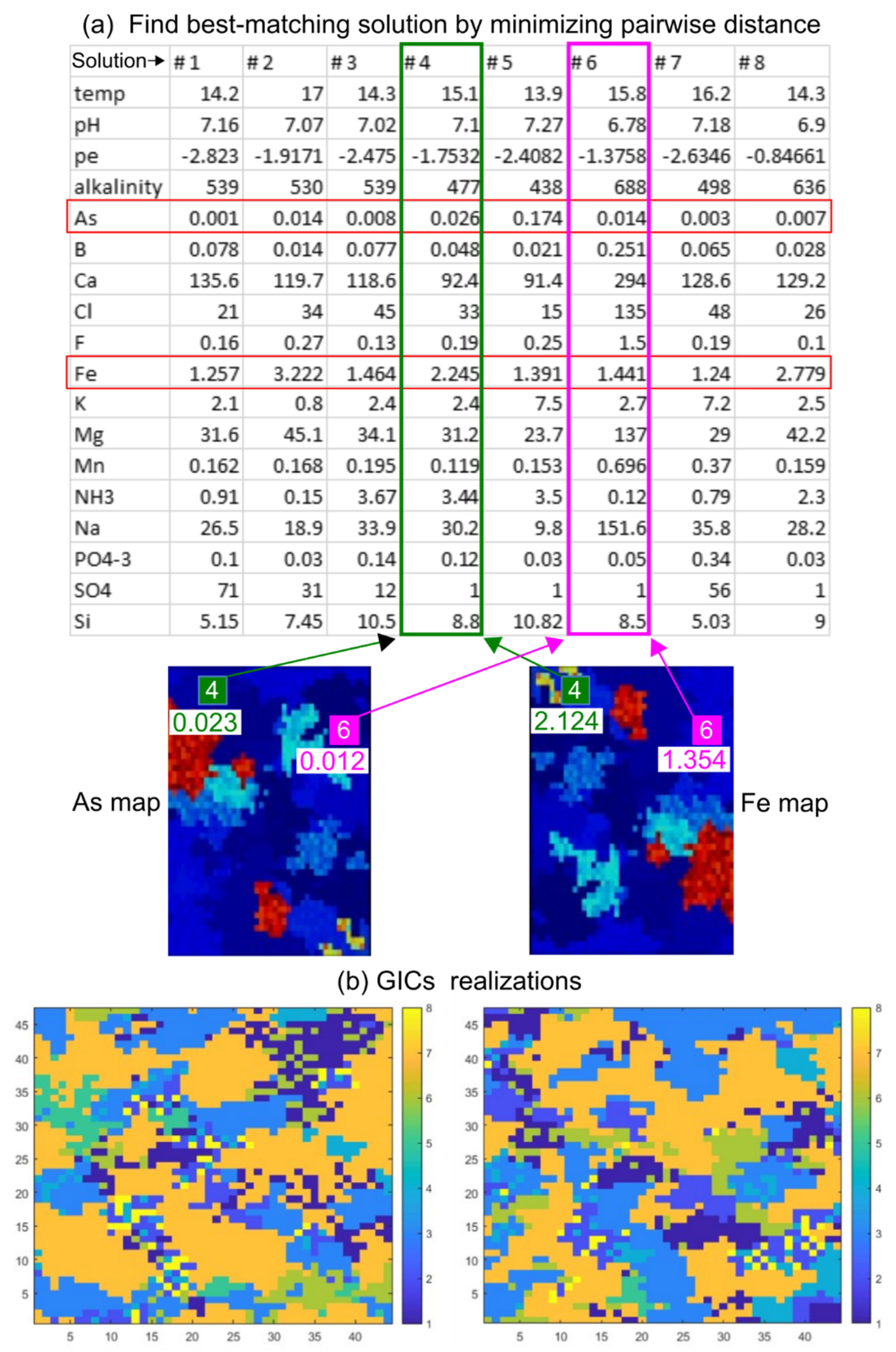
  • We treated the eight hydrogeochemical surveys performed in 2017 as eight PHREEQC “solutions”. We then created Nmc = 100 empty grids of the same size of the stochastic realizations (43 × 46 cells) and populated them with a unique solution in each grid cell. Such solution was chosen by minimizing, for each cell of each j-th pair of As and Fe realizations ( j = 1 , , N m c ), the pairwise Euclidean distance between the simulated As and Fe concentrations and the observed concentrations from the 8 PHREEQC solutions.
In this way, we obtained Nmc = 100 random maps of solutions (i.e., the geochemical initial conditions, GICs), which were used to populate the PHAST models. The mapping algorithm was coded through an in-house MATLAB script, which included the native pdist function to calculate pairwise Euclidean distance. The variograms and SIS computation was performed using SGEMS [45]. The resulting variograms are reported in the Supplementary Information SI-4.
An example of the approach is graphically depicted in Figure 4a. The map on the left represents a realization of As concentrations, while the map on the right represents a realization of Fe concentrations. In the cell marked by the green square, the SIS algorithm generated a concentration of As = 0.023 mgL−1 and of Fe = 2.214 mgL−1, shown respectively in the map on the left and on the right. The closest pairwise distance between measured and computed As and Fe concentrations in this specific cell correspond to the concentrations represented by the “Solution 4”. In the cell marked by the magenta square, the concentrations of As = 0.012 mgL−1 and Fe = 1.354 mgL−1 are instead closer to the “Solution 6”. For each cell (i.e., x-y position), we assigned the same solution in all layers, since the composition of the groundwater which is sampled by fully penetrating observation wells is an average aquifer composition of the entire borehole.
The process was repeated for each domain cell until the map of solution was completed. The whole procedure was then looped N m c = 1 00 times to obtain N m c = 1 00 solution maps. Examples of two solution maps obtained using this approach are shown in Figure 4b. Each of the N m c = 1 00 solutions maps were used to populate and run independent PHAST simulations. After each run, the entire spatial and temporal distribution of As and other key variables was stored. The ensemble of results was analyzed in a probabilistic fashion. For a generic variable X , the ensemble mean X ¯ and standard deviation σ X were computed to evaluate the change in time of the expected behavior of geochemical system under uncertainty. Empirical cumulative distribution functions (ecdfs) were computed and compared at different time scales to calculate the PNE above key thresholds of As concentrations.
We finally recalled that groundwater could be withdrawn through “fully penetrating” pumping wells, i.e., wells which are screened along the entire 12-m-long vertical section of the aquifer, or through partially penetrating well, and in particular through wells are screened at shallower depths. We postulated that a different pumping well configuration could result in a different PNE and become a useful decisional criterion for local administration, for instance to compute well-type-specific As risk for groundwater consumers. To demonstrate this, we conducted two distinct analyses:
  • A “full depth” analysis, where the statistics of As concentrations and other variables were calculated considering the entire model extension in the vertical direction.
  • A “shallow depth” analysis, where the same statistics were calculated for the top half of the model (i.e., up to 6 m), as a representative value for partially-penetrating pumping wells.

3. Results

3.1. Flow and Deterministic Transport Model

The subsurface lithological model created using spMC highlighted a large variability of lithological units within the WAA, both in terms of relative proportion and in terms of spatial continuity of such units. Volumetrically, the statistical analysis of available borehole logs (Figure 5a) indicates that about one third of the aquifer is composed of sandy materials (35% of the total volume), while the remaining two thirds are composed of fine-grained, low-permeable sediments (46% silt, 18% clay and 1% peat). The mean length of the materials along the x (i.e., E-W) direction shows (Figure 5b) similar lengths for sand and silt (respectively, 284 m and 297 m), while clay (122 m) and particularly peat (16 m) materials show shorter lengths. Comparing the lengths in the x direction with those computed for the y (N-S) direction (Figure 5c) reveals that sandy materials are quite isotropic in the horizontal direction, while silty material is slightly more anisotropic and elongated towards the x direction. Peat and particularly clay materials seem much more continuous along the y direction, when compared to the corresponding values in the x direction. For all materials, however, the mean lengths along the horizontal plane are much longer than in the vertical direction z (Figure 5d). Lengths of about 2 m were found for the sandy materials (the main aquifers of the WAA), with a ratio between the horizontal and vertical lengths close to 150.
The flow model indicates a mean groundwater velocity of about 0.2 m/d. The stratigraphic variation determines a spatial variability of the hydraulic parameters, which translates into a variability in the local flow velocity. Table 1 reports the resulting hydraulic parameters at the end of the calibration process. The sandy materials show a larger K than the finer-grained materials, suggesting that sandy horizons could be acting as preferential flow zones, enhancing the mixing between infiltrating waters and existing water. In the northern part of WAA, the calibrated recharge rates associated to the transient RCH BCs linearly decreased from an initial value of 10% of the total rainfall to 1% after 97 days and remained at 1% until the end of the simulation. In the southern and in the middle zones, the calibrated recharge rate linearly decreased from 10% to 3% after 60 days and remained at 3% until the end of the simulation. This range of values agrees with the recharge rates reported for the shallow aquifers of the adjacent Porto Marghera site [42].
Figure 6 shows the interpolated map of resulting head-level distribution at the end of the simulated period. It can be observed that the head levels are strongly affected by the presence of the drainage systems, which locally lower the water table below the sea level. At the stage depicted by this specific snapshot, the minimum head level is at −1.37 m above sea level (a.s.l.). Considering that the model elevation is 3 m a.s.l. and the layer discretization is 1 m, at the end of the simulated time the top four layers in the proximity of the drainage system are dry. As mentioned earlier, however, this issue does not imply a limitation for the reactive transport model, since the input mass flux associated to the recharge (a key mechanism for the control of As in our study) still applies to the top active layers.

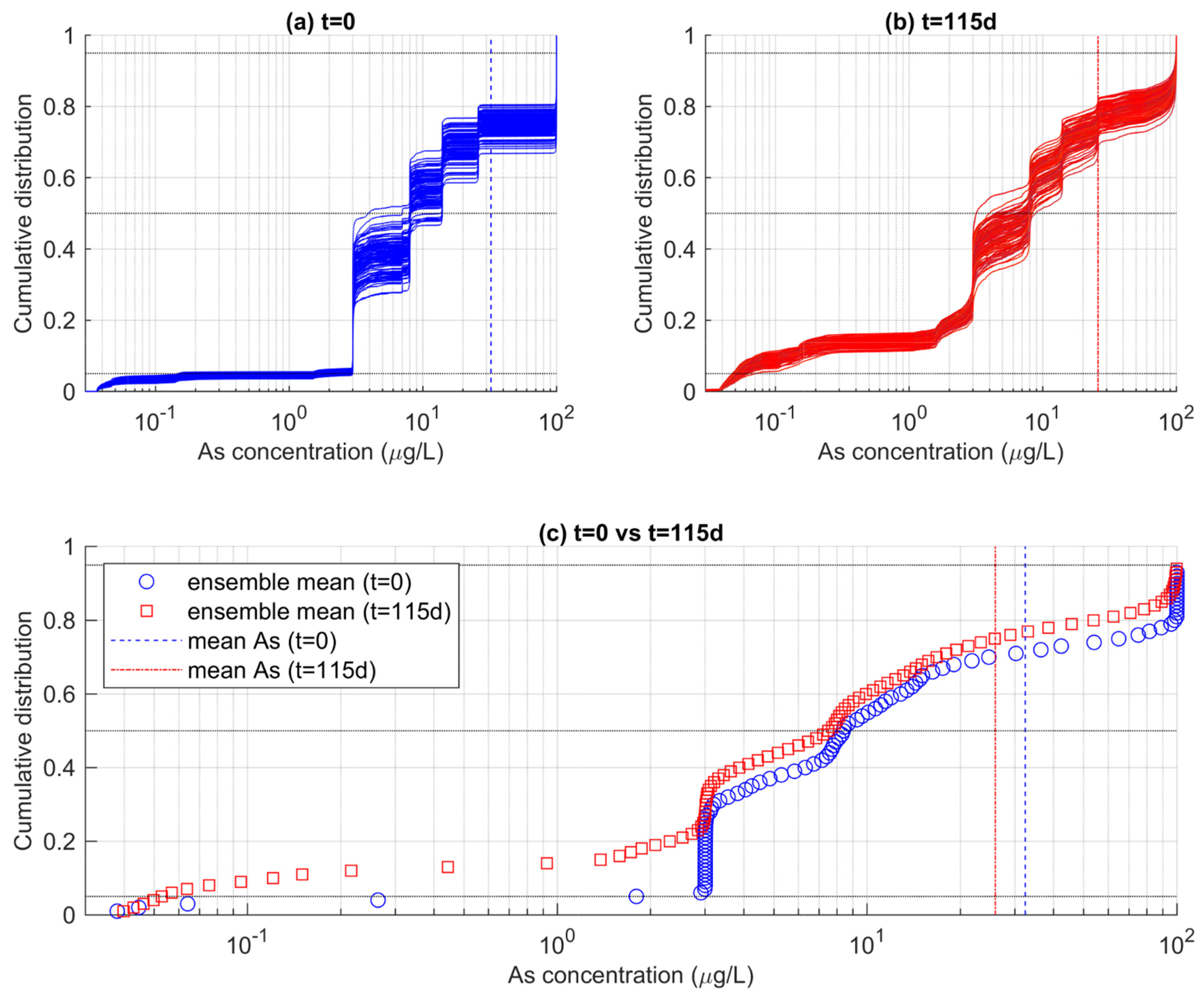
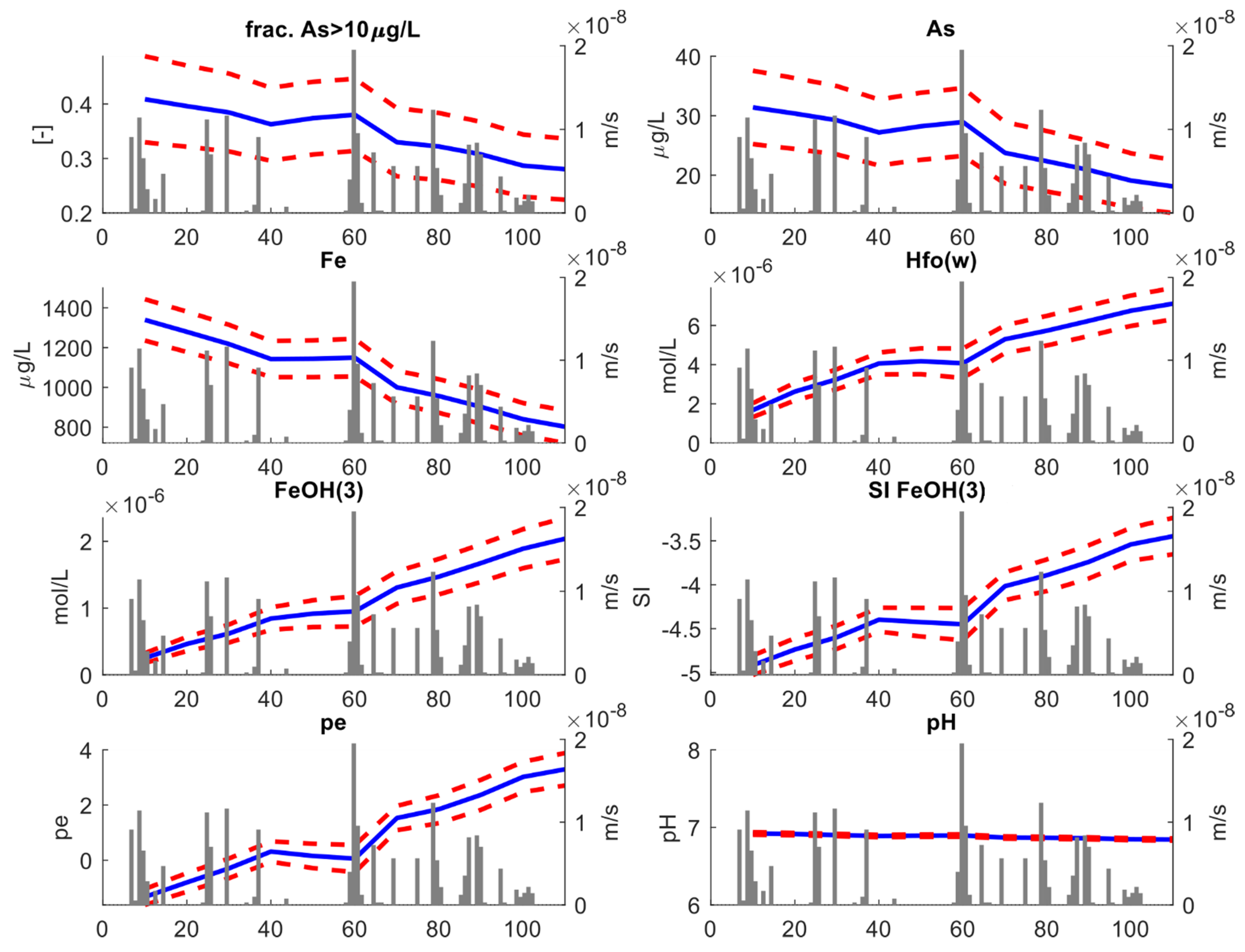
3.2. Stochastic Transport Model

3.2.1. Whole Aquifer Depth

We initially analyzed the statistical change in relevant geochemical species and variables at the scale of the entire model, i.e., considering the entire vertical extension of the aquifer. Key results of this analysis are shown in Figure 7. For each variable, the blue line represents the ensemble mean obtained from averaging over the 100 stochastic simulations, while the red dotted lines represent the 95% (±2σ) uncertainty envelope. The grey bars represent the recharge rates (ms−1), which are directly correlated to the rainfall events.
Our first significant result is the relative volumetric proportion (the fraction) of aquifer where As concentrations exceeding 10 μgL−1 decrease with time. Initially, ~43% of the entire aquifer is characterized by As concentrations above 10 μgL−1. As time elapses, the fraction drops toward a final value of ~39%. This behavior is linked to a decrease in average As concentration which tends to drop from ~32 μgL−1 to ~27 μgL−1. Although the model was not calibrated using geochemical information, the decreasing trend in As concentration simulated by the stochastic model is consistent with the previous results by DL2020. Since As and Fe are strongly correlated, dissolved Fe concentrations also drop with time, following a similar pattern as As concentrations. The drop in dissolved Fe is opposed to an increase in reactive surfaces (HFOs), whose amount depends directly on the amount of amorphous iron Fe(OH)3 existing in the system. The concentration of amorphous iron is inversely correlated to the amount of dissolved Fe. This is explained considering that, as the time proceeds, the ensemble mean of saturation index of Fe(OH)3 tends towards higher values, i.e., SI → 0. In other words, as time elapses the system tends towards equilibrium conditions for Fe(OH)3.
The main driver of such reduction is the aquifer recharge. This is demonstrated by the clear correlation between rainfall events and the oxidation reduction potential (ORP), here expressed by the pe = log ( e + ) . Initially, ORP tends to higher values; then, a sudden decrease in ORP is found at ~40 days, corresponding to the beginning of a dry period lasting several consecutive days. After that, new precipitation events occurred and ORP increased again. This is explained considering that precipitation triggers aquifer recharge, which adds oxidants to the aquifers. All the other redox-sensitive species displayed in Figure 7, including As, show a similar “bumped” behavior. Note instead that pH remains close to circumneutral conditions throughout the entire simulation time. This is consistent with the buffering of the calcite minerals.
Figure 8 shows the empirical cumulative distribution functions (ecdfs) of As concentrations obtained from two different time steps of the MRTM simulations. In Figure 8a, the ensemble of ecdf calculated for each realization reflects the distribution of As at the beginning of the simulation (t = 0). The ecdf indicates that the distribution of As in the whole aquifer is very heterogeneous. The use of the log scale helps to better capture the variations of As concentrations which span over more than three orders of magnitude and deviate largely from the mean value of ~32 μgL−1 (blue dotted vertical line). The shape of the ecdfs is alike among the different realizations. It is characterized by a stepwise increase in the cumulative probability, as a result of the SIS-based stochastic realizations used as GICs in the reactive transport models Figure 4. The SIS realizations include eight categories (i.e., the “solutions”), resulting in an equivalent number of steps, since each solution occupies a different proportion of the aquifer volume.
In Figure 8a, the ecdf reflects the distribution of As at the end of the simulation (t = 115 d). Note that the ensemble of ecdfs is now different than the ensemble of ecdfs calculated for t = 0. This is due to a combination of factors. First, transport determines a mixing among adjacent cells, such that the well-defined clustered As distribution at t = 0 is now more continuous, as reflected by smoother ecdf obtained at t = 115 d. Secondly, as time elapses, As is attenuated by the rainfall-driven redox-controlled adsorption on HFOs. Indeed, the ensemble of ecdfs at t = 115 d is shifted towards lower values, being consistent with the decrease in the mean As concentration to ~27 μgL−1.
These ecdf can be used to quantify the PNE of arsenic concentrations according to targeted thresholds. We note however that such estimation is hardly obtained from Figure 8a,b, where the ensemble of ecfds is quite spread. This is particularly true for values exceeding a concentration of 3 μgL−1. The ecfds spreading is explained considering that the relative proportion of As in the GICs is random outcome of the SIS algorithm. While on average all realizations embed the same statistics, each individual realization can produce a slightly different proportion of a specific solution. As such, we calculated the ensemble mean of the ecdfs to obtain a unique reference PNEs for the two analyzed times reported in Figure 8a,b.
The ensemble means of the ecdfs are reported in Figure 8c, along with the calculated mean As concentrations already reported in the previous panels. It was found that the expected PNE for the WHO-recommended threshold of 10 μgL−1 was 55% at t = 0, and increased to 60% at t = 115 d. This means that, on average, the fraction of aquifer that can be considered contaminated by arsenic at the end of the simulation was lower by 5% compared to the beginning of the simulation. For 50 μgL−1, another common threshold which is sometimes a maximum concentration in drinking water in countries such as Bangladesh, the probability of non-exceedance has increased from 71% at t = 0 to 78% at t = 115 d.
The time dependance of the PNE is consistent with the rest of the analysis and linked to the effect of As attenuation as controlled by the adsorption of HFOs. Attenuation increases as time elapses, as a consequence of the hypothesized effects of rainfall-controlled HFOs in the studied aquifer. Since PNE is directly connected to risk indicators, such as to compute the chronic exposure of population to an excess of a toxic waterborne compound, our results stress the importance of rainfall events as a critical aspect controlling the risk of As contamination in the studied area. This is important information for decision makers when quantifying the risk of As contamination in the studied area. Since the PNE is non-stationary in time, administrations should regularly update their risk calculations depending on new concentration levels.

3.2.2. Shallower Aquifer Portion

We now reanalyze the results from the stochastic models using a similar approach, this time focusing on the top six meters of the aquifers. Figure 9 shows the changes in the same geochemical species and variables evaluated in Figure 7. Compared to variation occurring when integrating the results of the entire aquifer thickness, we found a more marked decrease in As concentrations with time in the shallow portions of the aquifer. The relative aquifer fraction with As >10 μgL−1 dropped from 40% to 28%, which is linked to a decrease in average As concentrations from 31 μgL−1 at t = 0 to 20 μgL−1 at t = 115 d. A higher relative change was also observed for the other key parameters controlling As mobility.
The difference between the results of the shallower portions of the aquifer and those of the full aquifer is explained considering that the shallow aquifer is closer to the recharge boundary. Therefore, the recharge-driven redox changes are enhanced in the shallower parts of the aquifer than in the deeper part of it where groundwater remains more isolated from the ingress of oxidants. The relative control of recharge on As attenuation explains why the probability that As does not exceed a specific threshold also depends on the depth of the analyzed aquifer. Figure 10a,b show the ensemble of ecdfs for the top six meters of the aquifer calculated at t = 0 and t = 115 d, respectively, and Figure 10c the ensemble mean of these curves. While the distribution of As values at t = 0 is similar to the distribution calculated for the full-depth analysis (Figure 8c), at t = 115 d the ensemble-mean ecdf is smoother than in the previous case. The probability computed for different thresholds also changed. For As < 10 μgL−1, the probability increased from 58% at t = 0 to 70% at t = 115 d, while for As < 50 μgL−1, the PNE increased from 71%% at t = 0 to 86% at t = 115 d. Thus, the relative risk due to As excess in drinking water is more reduced if groundwater is withdrawn at shallower depths, owing to the better attenuating effects of rainfall-driven recharge on As.

4. Discussion

Stochastic modeling is a powerful method to compute the probability of non-exceedance (PNE) of toxic compounds in complex aquifers. While several models have been developed to compute the probability of As contamination in different environments [46], for groundwater such probability has been traditionally computed using data-driven statistical analysis [22]. For instance, the Bayesian Maximum Entropy theory was applied by Serre et al. [47] to study arsenic exposure across Bangladesh by the local population using a database that combined about 4000 tube-well and borehole samples from four different surveys and a total of 3373 As concentration measurements of the shallow aquifers. When such datasets do not exist, data-driven statistical analysis may be insufficient to perform probabilistic analysis.
The present study is among the first documented attempts to evaluate PNE for As critical concentrations in groundwater using a mechanistic MRTM formulation. Leveraging previous studies on the same area, the model accounted for key hydraulic and geochemical controls of As mobility in a shallow aquifer near Venice, Italy. Although stochastic mechanistic modeling coupled to geostatistical inference is a demonstrated tool that can generate probabilistic maps of time-dependent concentrations of toxic compounds [18,21], it is not clear why stochastic MRTM have not been widely documented so far in the literature. One reason may owe to the well-known computational burden required to resolve the nonlinear equations characterizing this type of model, which can determine very long computational times. A second reason may be linked to the number of unknowns and input parameters required to run MRTM. However, the present study showed that stochastic MRTM of As mobility can be computed with reduced computational burden (all simulations run overnight on a modern workstation) if the model embeds a simplified geochemical system that captures the essential mechanisms controlling As mobility.
Our stochastic analysis revealed that the shallow aquifers in the WAA are more sensitive to rainfall-controlled reactions than deeper parts of the aquifers. On the one hand, this corroborates and extends the validity of the conclusions by Dalla Libera et al. [29]. On the other hand, the results are well aligned with the conclusions from other studies that already identified a link between As mobility and aquifer recharge. Rodriguez et al. [48] explained the variation in As concentration in terms of the precipitation regime and the oxidation conditions induced by local rainfall incorporation. Our model results could be interpreted as if relatively shallow wells are less prone to generate As risk than relatively deeper wells. We stress the term “relative”, as this assessment refers uniquely to wells which are drilled up to a maximum depth of 10–15 m. In the Venice area, other aquifers located at much deeper depths exist and are utilized for drinking purposes.
It is also important to note that rainfall is not always linked to an attenuation of As concentrations. For instance, Duan et al. [49] found that rainfall implied an increase in As concentrations in Jianghan Plain in China. The authors suggested that rainfall could generate increasingly reducing conditions by increasing the groundwater table, while the dry season favors the ingress of oxidants and the adsorption of As of HFOs. Therefore, a sound evaluation of the site-specific mechanisms controlling As mobility is required prior to performing any stochastic MRTM.
Ultimately, we note that despite being based on a 3-D mapping of the subsoil, flow boundaries, recharge conditions, and the variations of the hydraulic parameters, the flow model was calibrated using the values of hydraulic heads measured in three aligned points, and the results were extended to the studied area. Future developments of the model should include more spatially distributed observation points, when available, in order to increase the validity of the model results.

5. Conclusions

We conducted a stochastic analysis based on multidimensional multicomponent reactive transport modeling (MRTM) to evaluate the probability that As does not exceed critical thresholds in the Western Agricultural Area (WAA). This area is a subset of the Venetian Alluvial Plain (VAP), near Venice (Italy), a densely populated region where As concentration in shallow Holocene aquifers (up to a depth of 10–15 m) exceeds the WHO-recommended threshold of 10 μgL−1. The complex spatial and temporal variations of As concentrations complicate the decisions regarding control and mitigation of As risk in the area.
The analysis suggested that the proposed modeling approach is able to quantify such probability. When the entire modeled aquifer is analyzed in a Monte-Carlo-based stochastic fashion, the relative proportion of the aquifer where As > 10 μg/L tends to decrease with time from an initial ~43% to a final ~39% after 115 simulated days. The probability of As non-exceedance increased from 55% to 60% with time using the 10 μgL−1 as target threshold, and from 71% to 78% when the target was 50 μgL−1. The result corroborates the conclusions of a previous study [29] who proposed that rainfall could add oxidants to the shallow aquifer and promote the formation of sorption surfaces, on which As can be temporarily removed from the aqueous environment.
When the same statistics are computed for the shallowest (top 6 m) portion of the aquifer, the relative aquifer fraction with As >10 μgL−1 dropped from 40% to 28% during the 115 simulated days, while the average As concentration dropped from 31 μgL−1 to 20 μgL−1. The PNE computed for different thresholds also changed when shallower parts of the aquifer were sampled compared to the full-aquifer sampling. For As < 10 μgL−1, the PNE increased from 58% to 70%, while for As < 50 μgL−1 the probability increased from 71% to 86%. Thus, the PNE was higher if groundwater was withdrawn at shallower depths. This is explained considering that the impact of rainfall on As attenuation is exacerbated in the shallower parts of the aquifer, since rainfall-controlled recharge has a more effective redox control in the shallower portions of the aquifer compared to the deeper parts.
We finally remark that the adopted modeling approach is general and can be applied to assess the risk of any toxic compound in complex systems. It can be easily extended to a different aquifer and/or to a different compound, provided that a mechanistic description of the processes controlling the mobility of the target variable are known.

Supplementary Materials

The following are available online at https://www.mdpi.com/article/10.3390/w13213086/s1, Supplementary SI-1: Datasets, sampling and analyses specifics; Supplementary SI-2: Stratigraphic dataset and transiograms; Supplementary SI-3: Flow model calibration; Supplementary SI-4: Variograms computed on the 2009 dataset.

Author Contributions

Conceptualization, all authors; methodology, N.D.L., D.P.; investigation, N.D.L., L.P.; resources, P.F.; data curation, D.P., N.D.L., G.C., Á.M.; writing—original draft preparation, all authors; project administration, P.F.; funding acquisition, P.F. All authors have read and agreed to the published version of the manuscript.

Funding

This research is part of a project that has received funding from the European Union’s Horizon 2020 research and innovation program under grant agreement No. 810980.

Institutional Review Board Statement

Not applicable.

Informed Consent Statement

Not applicable.

Data Availability Statement

All data used in this work are available in the Supplementary Information and at the Mendeley Repository https://data.mendeley.com/datasets/v4jm2txpfw/1 (accessed on 1 November 2021).

Acknowledgments

The results here presented have been developed in the frame of the MIUR Project “Dipartimenti di Eccellenza 2017—Le Geoscienze per la società: risorse e loro evoluzione”.

Conflicts of Interest

The authors declare no conflict of interest.

References

  1. Smedley, P.L.; Kinniburgh, D.G. Arsenic in Groundwater and the Environment. In Essentials in Medical Geology; Springer: Dordrecht, The Netherlands, 2013; pp. 279–310. [Google Scholar]
  2. Mueller, B. Results of the First Improvement Step Regarding Removal Efficiency of Kanchan Arsenic Filters in the Lowlands of Nepal—A Case Study. Water 2021, 13, 1765. [Google Scholar] [CrossRef]
  3. Podgorski, J.; Berg, M. Global Threat of Arsenic in Groundwater. Science 2020, 368, 845–850. [Google Scholar] [CrossRef] [PubMed]
  4. UNICEF Arsenic Primer: Guidance on the Investigation & Mitigation of Arsenic Contamination. UNICEF Water, Sanitation and Hygiene Section and WHO Water; Sanitation and Hygiene and Health Unit, United Nations Children’s Fund (UNICEF): New York, NY, USA, 2018.
  5. Fendorf, S.; Michael, H.A.; van Geen, A. Spatial and Temporal Variations of Groundwater Arsenic in South and Southeast Asia. Science 2010, 328, 1123–1127. [Google Scholar] [CrossRef] [PubMed] [Green Version]
  6. Smith, A.H.; Lingas, E.O.; Rahman, M. Contamination of Drinking-Water by Arsenic in Bangladesh: A Public Health Emergency. Bull. World Health Organ. 2000, 11, 1093–1103. [Google Scholar]
  7. Polya, D.; Charlet, L. Environmental Science: Rising Arsenic Risk? Nat. Geosci. 2009, 2, 383–384. [Google Scholar] [CrossRef]
  8. Gao, Z.P.; Jia, Y.F.; Guo, H.M.; Zhang, D.; Zhao, B. Quantifying Geochemical Processes of Arsenic Mobility in Groundwater From an Inland Basin Using a Reactive Transport Model. Water Resour. Res. 2020, 56, e2019WR025492. [Google Scholar] [CrossRef]
  9. Jakobsen, R.; Kazmierczak, J.; Sø, H.U.; Postma, D. Spatial Variability of Groundwater Arsenic Concentration as Controlled by Hydrogeology; Conceptual Analysis Using 2-D Reactive Transport Modeling. Water Resour. Res. 2018, 54, 10–254. [Google Scholar] [CrossRef]
  10. Appelo, C.A.J.; Postma, D. Geochemistry, Groundwater and Pollution; A.A. Balkema Publishers: London, UK, 2005. [Google Scholar]
  11. Battistel, M.; Stolze, L.; Muniruzzaman, M.; Rolle, M. Arsenic Release and Transport during Oxidative Dissolution of Spatially-Distributed Sulfide Minerals. J. Hazard. Mater. 2021, 409, 124651. [Google Scholar] [CrossRef]
  12. Postma, D.; Larsen, F.; Minh Hue, N.T.; Duc, M.T.; Viet, P.H.; Nhan, P.Q.; Jessen, S. Arsenic in Groundwater of the Red River Floodplain, Vietnam: Controlling Geochemical Processes and Reactive Transport Modeling. Geochim. Cosmochim. Acta 2007, 71, 5054–5071. [Google Scholar] [CrossRef]
  13. Rathi, B.; Neidhardt, H.; Berg, M.; Siade, A.; Prommer, H. Processes Governing Arsenic Retardation on Pleistocene Sediments: Adsorption Experiments and Model-Based Analysis. Water Resour. Res. 2017, 53, 4344–4360. [Google Scholar] [CrossRef]
  14. Sracek, O.; Bhattacharya, P.; Jacks, G.; Gustafsson, J.-P.; von Brömssen, M. Behavior of Arsenic and Geochemical Modeling of Arsenic Enrichment in Aqueous Environments. Appl. Geochem. 2004, 19, 169–180. [Google Scholar] [CrossRef]
  15. Ross, J.L.; Ozbek, M.M.; Pinder, G.F. Aleatoric and Epistemic Uncertainty in Groundwater Flow and Transport Simulation: UNCERTAINTY IN GROUNDWATER SIMULATION. Water Resour. Res. 2009, 45. [Google Scholar] [CrossRef]
  16. Michael, H.A.; Khan, M.R. Impacts of Physical and Chemical Aquifer Heterogeneity on Basin-Scale Solute Transport: Vulnerability of Deep Groundwater to Arsenic Contamination in Bangladesh. Adv. Water Resour. 2016, 98, 147–158. [Google Scholar] [CrossRef] [Green Version]
  17. Duan, Y.; Li, R.; Gan, Y.; Yu, K.; Tong, J.; Zeng, G.; Ke, D.; Wu, W.; Liu, C. Impact of Physico-Chemical Heterogeneity on Arsenic Sorption and Reactive Transport under Water Extraction. Environ. Sci. Technol. 2020, 54, 14974–14983. [Google Scholar] [CrossRef]
  18. Rubin, Y. Applied Stochastic Hydrogeology; Oxford University Press: New York, NY, USA, 2003. [Google Scholar]
  19. Tartakovsky, D.M. Assessment and Management of Risk in Subsurface Hydrology: A Review and Perspective. Adv. Water Resour. 2013, 51, 247–260. [Google Scholar] [CrossRef]
  20. Sanchez-Vila, X.; Fernàndez-Garcia, D. Debates—Stochastic Subsurface Hydrology from Theory to Practice: Why Stochastic Modeling Has Not yet Permeated into Practitioners? Water Resour. Res. 2016, 52, 9246–9258. [Google Scholar] [CrossRef] [Green Version]
  21. Pedretti, D.; Mayer, K.U.; Beckie, R.D. Controls of Uncertainty in Acid Rock Drainage Predictions from Waste Rock Piles Examined through Monte-Carlo Multicomponent Reactive Transport. Stoch Environ. Res. Risk Assess. 2020, 34, 219–233. [Google Scholar] [CrossRef]
  22. Ayotte, J.D.; Nolan, B.T.; Nuckols, J.R.; Cantor, K.P.; Robinson, G.R.; Baris, D.; Hayes, L.; Karagas, M.; Bress, W.; Silverman, D.T.; et al. Modeling the Probability of Arsenic in Groundwater in New England as a Tool for Exposure Assessment. Environ. Sci. Technol. 2006, 40, 3578–3585. [Google Scholar] [CrossRef] [PubMed]
  23. Dalla Libera, N.; Fabbri, P.; Mason, L.; Piccinini, L.; Pola, M. Geostatistics as a Tool to Improve the Natural Background Level Definition: An Application in Groundwater. Sci. Total Environ. 2017, 598, 330–340. [Google Scholar] [CrossRef] [Green Version]
  24. Lu, B.; Song, J.; Li, S.; Tick, G.R.; Wei, W.; Zhu, J.; Zheng, C.; Zhang, Y. Quantifying Transport of Arsenic in Both Natural Soils and Relatively Homogeneous Porous Media Using Stochastic Models. Soil Sci. Soc. Am. J. 2018, 82, 1057–1070. [Google Scholar] [CrossRef]
  25. Lorenz, E.N. Deterministic Nonperiodic Flow. J. Atmos. Sci. 1963, 20, 130–141. [Google Scholar] [CrossRef] [Green Version]
  26. Dalla Libera, N.; Fabbri, P.; Mason, L.; Piccinini, L.; Pola, M. A Local Natural Background Level Concept to Improve the Natural Background Level: A Case Study on the Drainage Basin of the Venetian Lagoon in Northeastern Italy. Environ. Earth Sci. 2018, 77, 487. [Google Scholar] [CrossRef]
  27. Carraro, A.; Fabbri, P.; Giaretta, A.; Peruzzo, L.; Tateo, F.; Tellini, F. Effects of Redox Conditions on the Control of Arsenic Mobility in Shallow Alluvial Aquifers on the Venetian Plain (Italy). Sci. Total Environ. 2015, 532, 581–594. [Google Scholar] [CrossRef] [PubMed]
  28. Carraro, A.; Fabbri, P.; Giaretta, A.; Peruzzo, L.; Tateo, F.; Tellini, F. Arsenic Anomalies in Shallow Venetian Plain (Northeast Italy) Groundwater. Environ. Earth Sci. 2013, 70, 3067–3084. [Google Scholar] [CrossRef]
  29. Dalla Libera, N.; Pedretti, D.; Tateo, F.; Mason, L.; Piccinini, L.; Fabbri, P. Conceptual Model of Arsenic Mobility in the Shallow Alluvial Aquifers near Venice (Italy) Elucidated through Machine Learning and Geochemical Modeling. Water Resour. Res. 2020, 56, e2019WR026234. [Google Scholar] [CrossRef]
  30. Parkhurst, D.L.; Appelo, C.A.J. Description of Input and Examples for PHREEQC Version 3—A Computer Program. For Speciation, Batch-Reaction, One-Dimensional Transport., and Inverse Geochemical Calculations; U.S. Geological Survey: Denver, CO, USA, 2013; p. 493.
  31. Parkhurst, D.L.; Kipp, K.L.; Engesgaard, P.; Charlton, S.R. PHAST—A Program for Simulating Ground-Water Flow, Solute Transport, and Multicomponent Geochemical Reactions; U.S. Geological Survey: Denver, CO, USA, 2004; p. 154.
  32. Charlton, S.R.; Parkhurst, D.L. Phast4Windows: A 3D Graphical User Interface for the Reactive-Transport Simulator PHAST. Groundwater 2013, 51, 623–628. [Google Scholar] [CrossRef]
  33. Kipp, J.L., Jr. Guide to the Revised Heat and Solute Transport. Simulator: HST3D—Version 2; U.S. Geological Survey (USGS) Water-Resources Investigation Report 97-4157; USGS: Denver, CO, USA, 1997.
  34. Fabbri, P.; Gaetan, C.; Sartore, L.; Dalla Libera, N. Subsoil Reconstruction in Geostatistics beyond Kriging: A Case Study in Veneto (NE Italy). Hydrology 2020, 7, 15. [Google Scholar] [CrossRef] [Green Version]
  35. Sartore, L. SpMC: Modelling Spatial Random Fields with Continuous Lag Markov Chains. R J. 2013, 5, 13. [Google Scholar] [CrossRef] [Green Version]
  36. Sartore, L.; Fabbri, P.; Gaetan, C. SpMC: An R-Package for 3D Lithological Reconstructions Based on Spatial Markov Chains. Comput. Geosci. 2016, 94, 40–47. [Google Scholar] [CrossRef] [Green Version]
  37. Carle, S.F.; Fogg, G.E. Transition Probability-Based Indicator Geostatistics. Math. Geol. 1996, 28, 453–476. [Google Scholar] [CrossRef]
  38. Ball, J.W.; Nordstrom, D.K. WATEQ4F—User’s Manual with Revised Thermodynamic Data Base and Test. Cases for Calculating Speciation of Major, Trace and Redox Elements in Natural Waters; Open-File Report; U.S. Geological Survey: Menlo Park, CA, USA, 1991.
  39. Dzombak, D.A.; Morel, F.M. Surface Complexation Modeling: Hydrous Ferric Oxide; John Wiley & Sons: New York, NY, USA, 1990. [Google Scholar]
  40. Gelhar, L.W.; Welty, C.; Rehfeldt, K.R. A Critical Review of Data on Field-Scale Dispersion in Aquifers. Water Resour. Res. 1992, 28, 1955–1974. [Google Scholar] [CrossRef]
  41. Goovaerts, P. Geostatistics for Environmental Applications; Oxford University Press: New York, NY, USA, 1997. [Google Scholar]
  42. Beretta, G.P.; Terrenghi, J. Groundwater Flow in the Venice Lagoon and Remediation of the Porto Marghera Industrial Area (Italy). Hydrogeol. J. 2017, 25, 847–861. [Google Scholar] [CrossRef]
  43. Journel, A.G. Fundamentals of Geostatistics in Five Lessons; Short Course In Geology; American Geophysical Union: Washington, DC, USA, 1989; Volume 8. [Google Scholar]
  44. Deutsch, C.; Journel, A. GSLIB: Geostatistical Software Library and User’s Guide; Oxford University Press: New York, NY, USA, 1998; 340p. [Google Scholar]
  45. Remy, N.; Boucher, A.; Wu, J. Applied Geostatistics with SGeMS. A User’s Guide; Cambridge University Press: New York, NY, USA, 2009. [Google Scholar]
  46. Georgopoulos, P.G.; Wang, S.-W.; Yang, Y.-C.; Xue, J.; Zartarian, V.G.; Mccurdy, T.; Özkaynak, H. Biologically Based Modeling of Multimedia, Multipathway, Multiroute Population Exposures to Arsenic. J. Expo. Sci. Environ. Epidemiol. 2008, 18, 462–476. [Google Scholar] [CrossRef]
  47. Serre, M.L.; Kolovos, A.; Christakos, G.; Modis, K. An Application of the Holistochastic Human Exposure Methodology to Naturally Occurring Arsenic in Bangladesh Drinking Water. Risk Anal. 2003, 23, 515–528. [Google Scholar] [CrossRef] [PubMed]
  48. Rodríguez, R.; Ramos, J.A.; Armienta, A. Groundwater Arsenic Variations: The Role of Local Geology and Rainfall. Appl. Geochem. 2004, 19, 245–250. [Google Scholar] [CrossRef]
  49. Duan, Y.; Gan, Y.; Wang, Y.; Deng, Y.; Guo, X.; Dong, C. Temporal Variation of Groundwater Level and Arsenic Concentration at Jianghan Plain, Central China. J. Geochem. Explor. 2015, 149, 106–119. [Google Scholar] [CrossRef]
Figure 1. (a) Geographical location of the Drainage Basin of Venice Lagoon (DBVL), which includes the studied area (WAA). Acronyms refer to the major cities of the Veneto regions. The arrow represents the regional-scale groundwater flow direction. (b) Conceptual not-to-scale vertical sketch of the stratified distribution of the main hydrofacies in the VAP. The trace of this section is parallel to the groundwater flow direction depicted in frame (a). Note that the amount of fine-grained sediments increases towards the Adriatic sea, forming the multilevel aquifer around the WAA. The figure has been modified after [26].
Water 13 03086 g001
Figure 2. (a) The model extension on top of the technical topographic map of the studied area, showing the position of the eight piezometers (“PZP”) monitored in the December 2017 campaign. The figure also shows the lateral flow boundary conditions (BCs), implemented as General Head Boundaries (“GHB”), and the drain (“DRN”). On the DRN, the numbers represent the nodes used to build the drain’s feature in the model. (b) The discretized mesh of the PHAST model, illustrating the position of the GHBs and DRN BCs as well as the zonation of the recharge (“RCH”) BCs.
Water 13 03086 g002
Figure 3. Subsurface lithological model of WAA created using spMC [36]. (a) Volume material distribution. (b) cross-sections, illustrating the position of the boreholes used to compute the transiograms and to condition the stochastic maps.
Water 13 03086 g003
Figure 4. (a) The example shows how pairs of As and Fe values are extracted from two specific cells on As (left) and Fe (right) random maps and associated to the closest PHREEQC solution (b) Two maps showing the distribution of PHREEQC solutions after completing the mapping in the whole domain. These maps represent the geochemical initial conditions (GICs) used to populate the stochastic PHAST models.
Water 13 03086 g004
Figure 5. (a) Relative volumetric proportion of the four “materials” in the modelled WAA. (bd) Box plots of the mean length of the four materials (in meters), respectively along the x, y and z direction.
Water 13 03086 g005
Figure 6. Simulated hydraulic head distribution within the WAA. The shown result refers to the end of the transient simulation after 115 days. The central zone is characterized by a depressed hydraulic head level as effect of the mechanical drainage system (green dotted line).
Water 13 03086 g006
Figure 7. Key results of the stochastic transport analysis. This figure refers to the “full depth” analysis. For each variable, the blue lines reproduce the ensemble mean obtained from averaging over the 100 stochastic simulations, while the red dotted lines represent the 95% (±2σ) uncertainty envelop. The gray bars represent the recharge rates (ms−1).
Water 13 03086 g007
Figure 8. Ensembles of ecdfs of As concentration calculated for the entire aquifer (a) at the beginning of the simulations (t = 0) and (b) at the end of the simulations (t = 115 d). In (c), the ensemble-mean ecdfs are reported, suggesting a time-dependent change in the probability that As does not exceed a specific threshold.
Water 13 03086 g008
Figure 9. Key results of the stochastic transport analysis. This figure refers to the “shallow depth” analysis. For each variable, the blue lines reproduce the ensemble mean obtained from averaging over the 100 stochastic simulations, while the red dotted lines represent the 95% (±2σ) uncertainty envelop. The gray bars represent the recharge rates (ms−1).
Water 13 03086 g009
Figure 10. Ensembles of ecdfs of As concentration calculated for the shallow (top six meters) of the aquifer (a) at the beginning of the simulations (t = 0) and (b) at the end of the simulations (t = 115 d). In (c), the ensemble-mean ecdfs are reported, suggesting a time-dependent change in the probability that As does not exceed a specific threshold.
Water 13 03086 g010
Table 1. Calibrated hydraulic parameters assigned to each material used in the model.
MaterialK (ms−1)Ss (m−1)Sy (-)
Sand1.25 × 10−41.00 × 10−72.00 × 10−1
Silt5.00 × 10−61.00 × 10−41.00 × 10−2
Clay1.00 × 10−85.00 × 10−45.00 × 10−3
Peat1.00 × 10−85.00 × 10−45.00 × 10−3
Publisher’s Note: MDPI stays neutral with regard to jurisdictional claims in published maps and institutional affiliations.

