Prediction of Nitrate and Phosphorus Concentrations Using Machine Learning Algorithms in Watersheds with Different Landuse

Abstract

Rapid industrialization and population growth have elevated the concerns over water quality. Excessive nitrates and phosphates in the water system have an adverse effect on the aquatic ecosystem. In recent years, machine learning (ML) algorithms have been extensively employed to estimate water quality over traditional methods. In this study, the performance of nine different ML algorithms is evaluated to predict nitrate and phosphorus concentration for five different watersheds with different land-use practices. The land-use distribution affects the model performance for all methods. In urban watersheds, the regular and predictable nature of nitrate concentration from wastewater treatment plants results in more accurate estimates. For the nitrate prediction, ANN outperforms other ML models for the urban and agricultural watersheds, while RT-BO performs well for the forested Grand watershed. For the total phosphorus prediction, ensemble-BO and M-SVM outperform other ML models for the agricultural and forested watershed, while the ANN performs better than other ML models for the urban Cuyahoga watershed. In predicting phosphorus concentration, the model predictability is better for agricultural and forested watersheds. Regarding consistency, Bayesian optimized RT, ensemble, and GPR consistently yielded good performance for all watersheds. The methodology and results outlined in this study will assist policymakers in accurately predicting nitrate and phosphorus concentration which will be instrumental in drafting a proper plan to deal with the problem of water pollution.

1. Introduction

With the current pace of industrialization and population growth, the concerns over water quality are very sensitive at present [1]. The demand for water has increased because of the growing population and development activities. On the other hand, the level of pollution in water sources has also increased significantly [2].

Nitrate and phosphate compounds are commonly used as industrial chemical reagents and in chemical fertilizers. Higher amounts of nitrate and phosphate can have an adverse effect not only on the water resources but also on the surrounding ecosystem. Proper management of these chemicals is important in large water bodies to mitigate the harmful impact on the aquatic ecosystem. Machine learning (ML) models can be effectively employed to model the nitrate and phosphorus distribution and predict its concentration in the water system. The ability to predict nitrate and phosphorus concentration accurately can provide engineers and policymakers with a proper plan to deal with the problem. These nutrients need to be measured over multiple locations due to the distributed nature of the water networks. However, measuring daily nutrient concentrations across stream cross-sections is both arduous and expensive. Consequently, most hydrological monitoring programs measure streamflow and nutrient concentrations less frequently (such as weekly or monthly), supplemented by storm sampling to better quantify nutrient movement during high-flow periods [3].

Ahmed et al. [4] used wavelet denoising technique (WDT) combined with ML to predict various quality parameters. Over the last decade, the methods for forecasting various water quality indicators have advanced. Heuvelmans et al. [5] forecasted nitrate concentration on a daily basis using a regression equation. While various ML models have been tested in recent years for the most reliable forecast, the most used techniques capable of predicting missing nitrate and phosphorus concentrations are artificial neural network (ANN), k-nearest neighbor (kNN), support vector machine (SVM), regression tree (RT), random forest (RF), and reduced error pruning tree (REPTree) [3,6,7,8,9,10,11].

ANN has been one of the most accurate models for nutrient concentration prediction. Anctil et al. [12] reported that two and three input MLP models based on the neural network could predict the daily nitrate concentration of a 7.1 square kilometer urban agricultural basin near Paris with 90% and 75% accuracy, respectively. Yu et al. [13] developed a MLP model to estimate nitrate loading that accounted for 80% of the variance in daily streamflow and nitrate loads, with better efficacy than linear regression (LR). Additional studies have confirmed that for similar nutrient loading/concentration prediction, MLP is more efficient than traditional methods [14,15,16,17]. Poor and Ullman [18] compared the performance of the regression tree (RT) and multiple linear regression (MLR) methods to predict the yield of nitrate and chloride ions in 71 watersheds in the Willamette River Basin. The results demonstrate that the RT can result in a high $R^2$ in all types of watersheds. However, the learning speed of the MLP is slow and tends to fall into the local extremum leading to partial training and learning [19]. Therefore, it is necessary to test and validate the performance of MLP method for the prediction of water quality.

The kNN algorithm can also achieve excellent results [20,21,22]. Towler et al. [23] used a kNN bootstrap approach to accurately simulate the variability in the influent water quality data from a drinking water treatment plant with respect to observed data. Li et al. [24] used both kNN and principal component analysis (PCA) to forecast nutrient profile from an agricultural watershed and found both algorithms to be equally accurate. The algorithm, however, is sensitive to outliers, as it simply selects the neighbors based on Euclidean distance, such that missing values also cause considerable biases in the prediction. For unevenly distributed data, the algorithm may be biased towards the category with large data and ignore the one with a smaller number of data points [25].

LR is the simplest and intuitive regression model; hence, it is taken as the reference baseline method to predict nutrient concentration. After an extensive literature study, it is observed that the classification tree-based methods [8,9] and cluster-based methods [6,7,11] are the two most used methods in predicting the nutrient concentration. So, three classification tree-based models: RT, RF, and the ensemble model, and two cluster-based ML models: kNN and ANN are employed to predict nutrient concentration. In addition to the above-mentioned ML models, the performance of two kernel-based models: SVM and Gaussian process regression (GPR) [7,10] are also evaluated. Hence, in this study, the performance of different machine learning algorithms is evaluated over multiple watersheds (Cuyahoga, Grand, Maumee, Raisin, and Sandusky) draining into Lake Erie in the United States. The major objectives of the study include

• The analysis of concentration–discharge (C–Q) relationship for different type of watersheds;
• To assess the applicability of BO to optimize hyperparameters of RT, ensemble, and GPR to predict nitrate and phosphorus concentration;
• The performance evaluation of nine different ML algorithms for the nitrate and phosphorus prediction.

The paper is arranged in the following order: Section 2 outlines the methodology employed in the study with a brief description of the study area, ML algorithms and parameter settings for the training and test set, Section 3 incorporates relevant results with appropriate discussions, and Section 4 concludes the study.

2. Materials and Methods

2.1. Study Area and Data Structure

In this study, the water quality data were collected from five watersheds: Cuyahoga, Grand, Maumee, Raisin, and Sandusky, draining into Lake Erie (Figure S1—Supplementary Materials). These five basins have similar climate, soil, ecoregion, and cropping systems and are also located very close to each other. National Center for Water Quality Research (NCWQR) maintains long-term daily time-series datasets for these watersheds [26]. The water quality depends on the physical and anthropogenic features of the watershed; hence, watersheds with different land-use distributions are selected in this study. As per NCWQR, Cuyahoga is an urban watershed (39.54% urban and 33.55% forest), Grand is a forested watershed (50.10% forest and 40% agricultural), while Maumee (73.33% agricultural), Raisin (49.56% agricultural), and Sandusky (77.59% agricultural) are predominantly agricultural watersheds (Table S1—Supplementary Materials). The water quality does not change drastically for an urban watershed, so the data structure is simple and consistent [3]. On the contrary, agricultural watershed experiences an influx of nutrients deposited in the soil during the high flow season, so the water quality response is partially seasonal. Likewise, the water quality response from the forest watershed can be entirely seasonal.

The long-term daily streamflow data were obtained from the United States Geological Survey (USGS) website (https://waterdata.usgs.gov/nwis/rt, accessed on 14 October 2021) and nitrate, total suspended solids, and total phosphorus concentration were obtained from the NCWQR at Heidelberg University. The total data points used in this study are 11,996 for Cuyahoga, 5049 for Grand, 12,849 for Maumee, 9241 for Raisin, and 11,468 for Sandusky. The streamflow and water quality samples were collected daily at the outlet of each watershed, supplemented by more frequent samplings (up to three per day) during high-flow periods. Hence, daily average streamflow and concentration values were used in this case. The preliminary data cleaning was performed to remove the observation with negative streamflow and concentrations.

Descriptive statistics of parameters for all watersheds are provided in Table S2 (Supplementary Material). The agricultural Maumee watershed ($16,395{\mathrm{km}}^2$) is the largest watershed considered in this study, followed by Sandusky ($3239{\mathrm{km}}^2$) and Raisin ($2698{\mathrm{km}}^2$). Hence, the Maumee watershed had the highest mean streamflow of $180.27{\mathrm{m}}^3/\mathrm{s},$ which is expected because of its large size. The urban Cuyahoga watershed resulted in the highest mean total suspended solids concentration of $102.627\mathrm{mg}/\mathrm{L}$, which can be attributed to construction activities in the urban areas. Likewise, the highest mean nitrate ($4.192\mathrm{mg}/\mathrm{L})$ and total phosphorus ($0.236\mathrm{mg}/\mathrm{L})$ concentrations were observed in the agricultural Maumee watershed. The standard deviation of streamflow for Maumee is very high, indicating that the streamflow varies significantly throughout the year for this watershed. The same is the case for total suspended solids in the Cuyahoga and total phosphorus and nitrate concentration in the Sandusky.

2.2. Machine Learning Algorithms

In this study, MATLAB R2020a [27] is used to implement all ML algorithms. Likewise, linear regression (LR) is taken as the reference method to estimate nitrate and phosphorus concentration for all watersheds.

2.2.1. Linear Regression (LR)

LR fits the data with a linear equation, i.e., polynomial equation of first order. This modeling is useful for data having linear relations. The typical linear regression model can be mathematically modeled as:

$$\widehat{Y}=\sum \left(aX+b\right)$$

(1)

where $X$ and $\widehat{Y}$ represent the input and output variable, respectively. The least-square method is employed to fit the model coefficients ($a$ and $b$) using the actual and the predicted data.

2.2.2. k Nearest Neighbors (kNN)

kNN models are based on the proximity of data points where a new object is classified based on features and training patterns [28]. Here, the output or the forecasted value is the average or the specified number of neighboring values. The specified number is described as the value k. The algorithm for kNN is:

• Initialize k;
• Calculate the Euclidean distance of the query example to the labeled examples

$$d\left(x,x^{\prime }\right)=\sqrt{{\left(x_1-x_1^{\prime }\right)}^2+{\left(x_2-x_2^{\prime }\right)}^2+\cdots +{\left(x_n-x_n^{\prime }\right)}^2}$$

(2)

where, $\left(x,x^{\prime }\right)$ is the sample point;

• Sort the labeled examples from smallest to largest;
• Find an optimal number k of nearest neighbors based on RMSE using cross validation;
• Compute an inverse weighted average with kNN.

2.2.3. Regression Tree (RT)

A RT is an approach to nonlinear regression, which is built through recursive partitioning. Recursive partitioning is an iterative process of splitting the data into more manageable partitions and again splitting each partition into smaller sub-divisions. RT represents recursive partitioning in the form of a tree with each terminal node representing a cell of the partition. RT is simple to model and visualize, but the unstable nature of a single tree model resulted in the development of ensembles.

2.2.4. Ensemble

Ensemble methods combine a number of weak RT models to form a more accurate RT model. Ensembles create multiple diverse regression models by taking different samples of the original data set and then combining their output. Two types of ensembles: Bagging and Least-Squares Boosting (LSBoost) are used in this study.

Random sampling with replacement is employed in Bagging to generate numerous training sets. RT algorithm is applied to each data set, and then the average of the models is taken to compute predictions for the unseen data.

A more accurate model is generated in Boosting by successively training models to concentrate on records with poor prediction in previous models. All predictors are combined by a weighted majority vote after completion. A new learner is fitted to the difference between the observed response and the aggregated prediction of all learners grown previously by the ensemble in LSBoost.

2.2.5. Random Forest (RF)

Another type of ensemble employed in this study is a RF. RF constructs a number of decision trees which is used to classify a new instance by the majority vote. A subset of randomly selected attributes from the original set is used by each decision tree node. Likewise, a different bootstrap sample data is used by each tree, such as that of Bagging. The number of trees generated in RF might range from hundreds to thousands. In this study, the number of trees is selected to be ten to construct a forest.

2.2.6. Artificial Neural Network (ANN)

ANN uses connected units between input and output layers to resolve a complex problem. Among several ANN topologies, MLP is employed in the current study. The connected unit is generally a simple linear equation, and the output layer uses an activation unit, which makes it very different from the polynomial regression. The activation unit acts as a logical switch that is activated only for threshold values. Some common types of activation functions are Sigmoid and ReLu. This study uses ReLu activation. Typical MLP with a hidden layer can be mathematically modeled as:

$$y_i={\sum }_j^n{w}_{i,j}{x}_j+b$$

(3)

where, x is the input, w is the weight, and b is the bias in hidden layer.

2.2.7. Support Vector Machine (SVM)

SVM based regression model is useful for modeling complex relations, which are not easily described by lower-order polynomial equations. SVM is a powerful supervised learning technique with excellent generalization ability because of which it is extensively utilized for solving problems regarding pattern recognition, classification, regression, and prediction [29]. The predicted value is obtained using the equation:

$$\widehat{Y}={\sum }_{i=1}^{n}K\left(X_i,X_0\right)\left({\alpha }_i-{\alpha }_i^{*}\right)$$

(4)

where ${\alpha }_i$ and ${\alpha }_i^{*}$ are the support vectors and $K\left(X_i,X_0\right)$ is the kernel function. SVM function can be used with various kernel functions (KF) to implement its regression learner. The application of the gaussian kernel function (GKF) is popular with SVM classification and regression which is defined as:

$$K\left(X_i,X_0\right)=\mathit{exp}\left(\frac{-{\left|\left|x_i-x_j\right|\right|}^2}{2{\sigma }^2}\right)$$

(5)

In this study, fine Gaussian SVM (F-SVM) and medium Gaussian SVM (M-SVM) is used. Medium and fine gaussian is defined based on the slenderness of the gaussian function being used.

2.2.8. Gaussian Process Regression (GPR)

GPR is a non-parametric model which works on the principles of Bayesian probability. GPR can be applied through various methods with variations in kernel type, kernel function basis function, etc. In this study, Nonisotropic Exponential, Nonisotropic Matern 3/2, Nonisotropic Matern 5/2, Nonisotropic Rational Quadratic, Nonisotropic Squared Exponential, Isotropic Exponential, Isotropic Matern 3/2, Isotropic Matern 5/2, and Isotropic Squared Exponential kernels are applied. Constant, Zero, and Linear basis functions are employed in the implementation.

2.3. Experimental Configuration

The entire dataset was divided into two sets for each watershed; an initial 70% of the data was utilized for training ML models, and the rest 30% was employed for the model assessment. A five-fold cross validation method was employed during the model development to prevent model overfitting in the training set. Daily measured streamflow and month (representing the seasonal characteristic) were taken as independent variables to predict nitrate concentration. As most of the total phosphorus is particulate phosphorus attached to suspended solid particles, total suspended solid was also taken as an independent variable alongside streamflow and month to predict total phosphorus concentration. Detailed parameters for each ML algorithm are illustrated in Table S3 (Supplementary Materials).

2.4. Bayesian Optimization (BO)

BO is a hyperparameter search method applied in ML problems by minimizing a particular objective function [30]. Based on the past evaluation results of the objective function, an alternate function is established with BO to minimize its value. In comparison to random grid search, BO refers to past evaluation results when selecting parameters in each iteration which greatly saves search time and improves optimization efficiency. Mean squared error (MSE) is taken as an objective function for this study. While minimum leaf size is the only hyperparameter to be optimized in the RT model, ensemble method, minimum leaf size, number of learners, learning rate, and number of predictors to sample are to be optimized in the ensemble method. Likewise, sigma, basis function, kernel function, kernel scale, and standardization are the hyperparameter to be optimized in the GPR model. The hyperparameters and search spaces of RT, ensemble, and GPR are listed in Table S4 (Supplementary Materials).

2.5. Evaluation Metrics

Following statistical indicators namely, coefficient of determination ($R^2$), root mean square error (RMSE), and mean absolute error (MAE) is utilized to evaluate the performance of various models. The model performance is evaluated using the equations given below [31]:

$$R^2=\frac{{\left[{\sum }_{i=1}^m\left(X_i-\overline{X}\right)\left(Y_i-\overline{Y}\right)\right]}^2}{{\sum }_{i=1}^m{\left(X_i-\overline{X}\right)}^2{\sum }_{i=1}^m{\left(Y_i-\overline{Y}\right)}^2}$$

(6)

$$\mathrm{MSE}=\frac{1}{m}{\sum }_{i=1}^m{\left(Y_i-X_i\right)}^2$$

(7)

$$\mathrm{RMSE}=\sqrt{\frac{1}{m}{\sum }_{i=1}^m{\left(Y_i-X_i\right)}^2}$$

(8)

$$\mathrm{MAE}=\frac{1}{m}{\sum }_{i=1}^m\left|Y_i-X_i\right|$$

(9)

where, $X_i$ and $Y_i$ represent the measured and predicted values; while $\overline{X}$ and $\overline{Y}$ represent the average measured and average estimated values. $m$ is the number of data points.

$R^2$ indicates the variance of the dependent variable that is explained by independent variables. RMSE value indicates the short-term performance of the model. A lower RMSE value corresponds to better performance. Similarly, MAE indicates the magnitude of error one can expect from the forecast on an average without considering their direction. The combination of RMSE and MAE can be used to analyze the variation of errors in the forecast. The RMSE is always greater than or equal to MAE, and the greater difference between them indicates the greater variance in the individual errors of the forecast.

3. Results and Analysis

3.1. Impact of Watershed Characteristics on Prediction

Concentration–discharge (C–Q) relationships for each watershed are given in Figure S2 (Supplementary Materials). In regard to the nitrate concentration, the slope of the C–Q regression line (b) for the Cuyahoga was negative, while that of the other four watersheds was positive. This indicates that the nitrate concentration essentially dilutes with the increasing streamflow in Cuyahoga. On the contrary, the nitrate concentration increases along with the streamflow in the other four watersheds. In an urban watershed, such as the Cuyahoga, the point sources such as wastewater treatment plants are the primary source of nitrate, which can be quickly diluted by storm events [3,32]. In agricultural areas, however, increased flow can flush the nitrate deposited in the soil, resulting in the elevated nitrate concentration. In this case, a more severe event can result in more nitrate loss in water, which is similar to the situation in a forested watershed.

In regard to the total phosphorus concentration, the slope of the C–Q regression line (b) for all five watersheds was positive. Suspended solids are generated from nonpoint sources from agricultural lands and construction areas. Likewise, increased streamflow can flush the sediment and associated soil particles and increase suspended solids concentration in the water column. As most of the total phosphorus is particulate phosphorus attached to suspended solid particles, the total phosphorus concentration increases during storm events [2]. Hence, the total phosphorus concentration increases along with the streamflow irrespective of the type of watershed. The larger slope ‘b’ indicates that the concentration has more reaction with the streamflow [33].

3.2. Relative Performance of ML Algorithms to Predict Nitrate Concentration

3.2.1. Model Development

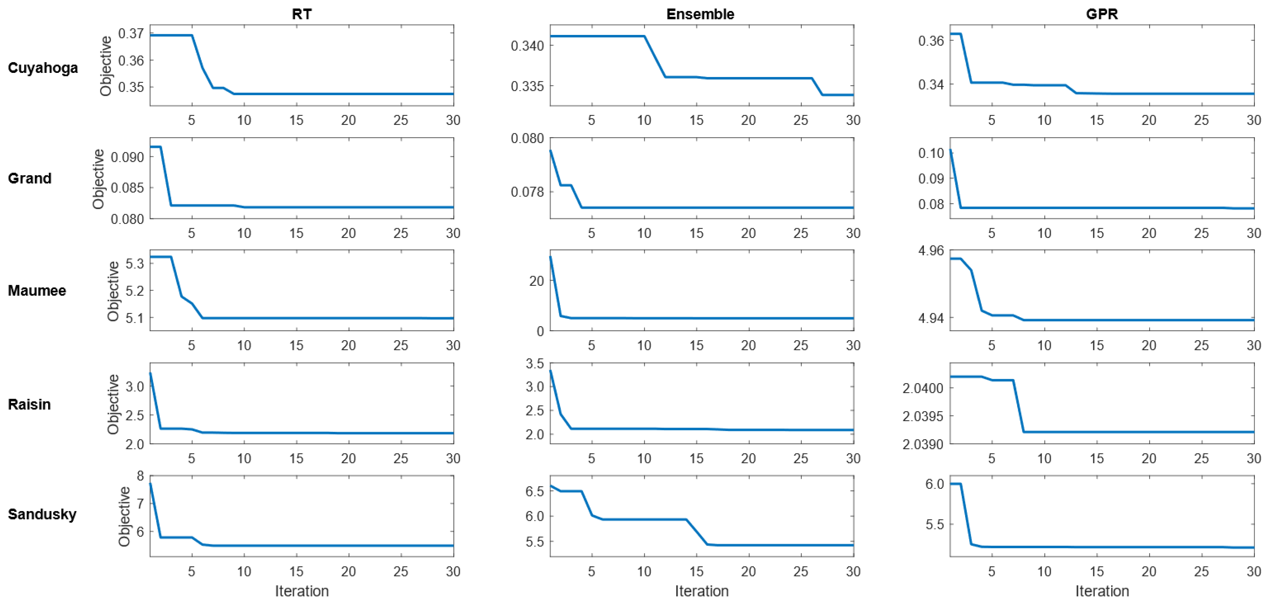
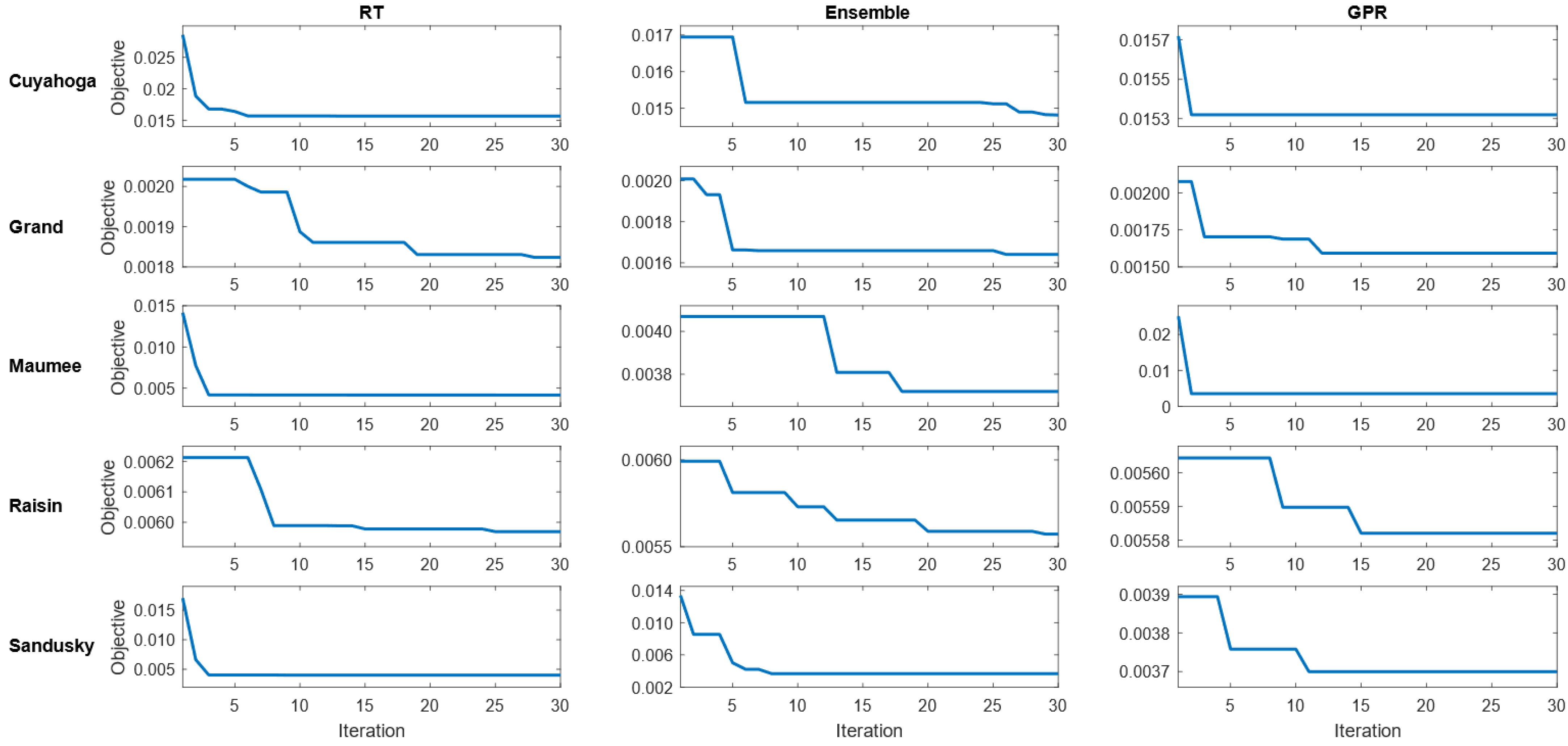
In this study, Bayesian optimized RT, Ensemble, and GPR models were run for 30 iterations during the model development, and the convergence of objective function in the iterative process is illustrated in Figure 1. For the Cuyahoga watershed, GPR converged to the minimum objective of 0.3355 after $13\mathrm{th}$ iteration. Hence, BO is more effective in improving GPR compared to RT and Ensemble for the Cuyahoga watershed. Likewise, BO is more effective in improving GPR compared to RT and Ensemble for Maumee (4.9569), Raisin (2.0403), and Sandusky (5.4210). On the contrary, BO is more effective in improving ensemble compared to RT and GPR for the Grand watershed with the objective of 0.0788. The result of Bayesian optimized hyperparameters in RT, ensemble, and GPR models for nitrate prediction are shown in

Table 1. Result of Bayesian optimized hyperparameters in RT, ensemble, and GPR models for nitrate prediction.

Algorithm	Parameter	Cuyahoga	Grand	Maumee	Raisin	Sandusky
RT	Minimum leaf size	73	83	72	54	51
Ensemble	Ensemble method	Bag	LSBoost	LSBoost	LSBoost	Bag
	Minimum leaf size	58	39	39	2	80
	Number of learners	10	10	10	12	10
	Learning rate	-	0.57165	0.65104	0.3731	-
	Number of predictors	2	2	2	2	2
GPR	Sigma	10.491	3.3665	0.077995	22.7795	30.6111
	Basis function	Constant	Zero	Linear	Zero	Zero
	Kernel function	Nonisotropic Exponential	Nonisotropic Rational Quadratic	Nonisotropic Exponential	Nonisotropic Matern 3/2	Nonisotropic Exponential
	Kernel scale	47.9729	11,091.2258	4054.6778	22.7014	7039.0333
	Standardize	TRUE	FALSE	TRUE	TRUE	TRUE

.

Table 2. Comparison of $R^2$, RMSE, and MAE using different ML algorithms for nitrate prediction on training dataset.

Watershed	Parameter	LR	F-SVM	M-SVM	kNN	RF	ANN	RT-BO	Ensemble-BO	GPR-BO
Cuyahoga	$R^2$	0.41	0.75	0.74	0.70	0.71	0.75	0.75	0.75	0.76
	RMSE	0.9026	0.5887	0.5997	0.6470	0.6330	0.5850	0.5894	0.5846	0.5792
	MAE	0.7088	0.4183	0.4266	0.4730	0.4620	0.4210	0.4259	0.4211	0.4168
Grand River	$R^2$	0.05	0.27	0.21	0.03	0.19	0.31	0.28	0.31	0.30
	RMSE	0.3287	0.2890	0.2988	0.3420	0.3030	0.2800	0.2861	0.2808	0.2814
	MAE	0.2434	0.1914	0.1983	0.2460	0.2100	0.1970	0.2003	0.1964	0.1962
Maumee	$R^2$	0.12	0.49	0.45	0.26	0.39	0.52	0.50	0.51	0.51
	RMSE	2.9846	2.2875	2.3591	2.7370	2.490	2.2230	2.2580	2.2382	2.2264
	MAE	2.3930	1.5890	1.6711	2.0240	1.7860	1.6070	1.6403	1.6249	1.6142
Raisin	$R^2$	0.23	0.59	0.56	0.46	0.53	0.62	0.59	0.61	0.62
	RMSE	2.0289	1.4755	1.5265	1.6970	1.5890	1.4250	1.4787	1.4461	1.4284
	MAE	1.4971	0.9628	0.9967	1.1620	1.0890	0.9780	1.0208	0.9909	0.9807
Sandusky	$R^2$	0.10	0.48	0.41	0.30	0.38	0.52	0.50	0.51	0.51
	RMSE	3.1481	2.4046	2.5503	2.7740	2.6140	2.3130	2.3467	2.3326	2.3283
	MAE	2.4705	1.6156	1.7488	1.9610	1.8080	1.6390	1.6676	1.6595	1.6505

illustrates the fitting statistics of different ML models for nitrate prediction on the training dataset. For the urban Cuyahoga watershed, F-SVM, M-SVM, ANN, RT-BO, ensemble-BO, and GPR-BO performed reasonably well in explaining the variance of nitrate concentration. Among these models, GPR-BO performs better than other ML models with $R^2$ of 0.76, RMSE of 0.5792 $\mathrm{mg}/\mathrm{L}$, and MAE of 0.4168 $\mathrm{mg}/\mathrm{L}$ for the training set. Likewise, ensemble-BO ranks second with $R^2$ of 0.75 and RMSE of 0.5846 $\mathrm{mg}/\mathrm{L}$.

On the contrary, for the forested Grand watershed, all the ML models showed mediocre performance with ANN ($R^2=0.31$ and RMSE = 0.2800 $\mathrm{mg}/\mathrm{L}$) being the best performing model regarding the $R^2$ and RMSE. For the agriculture dominated watersheds (Maumee, Raisin and Sandusky), F-SVM, M-SVM, ANN, RT-BO, ensemble-BO, and GPR-BO again showed acceptable performance, which was lower than that of the Cuyahoga but better than the Grand. For the agricultural watersheds of Maumee, Raisin and Sandusky, ANN was the best performing model followed by GPR-BO regarding the $R^2$ and RMSE. Among the agricultural watersheds, the model predictability was comparatively higher for the Raisin. It was also observed that all ML models significantly outperforms traditional LR model in predicting nitrate concentration for the training dataset.

A comparison of statistical indicators showed that $R^2$, RMSE, and MAE, at times, followed a different trend. For the urban Cuyahoga watershed, all statistical indicators followed the same trend as the GPR-BO has the maximum $R^2$ and the minimum RMSE and MAE. For the agricultural and forested watersheds, ANN has the maximum $R^2$ and the minimum RMSE whereas F-SVM has the minimum MAE. Also, reasonable difference between the RMSE and MAE indicates that the variance in the individual errors of the forecast is acceptable.

3.2.2. Model Testing

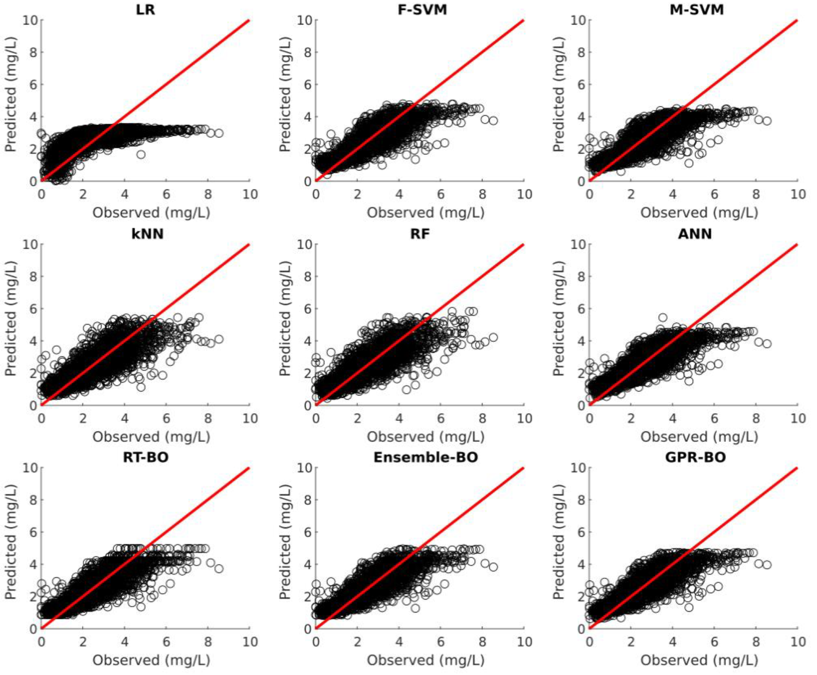
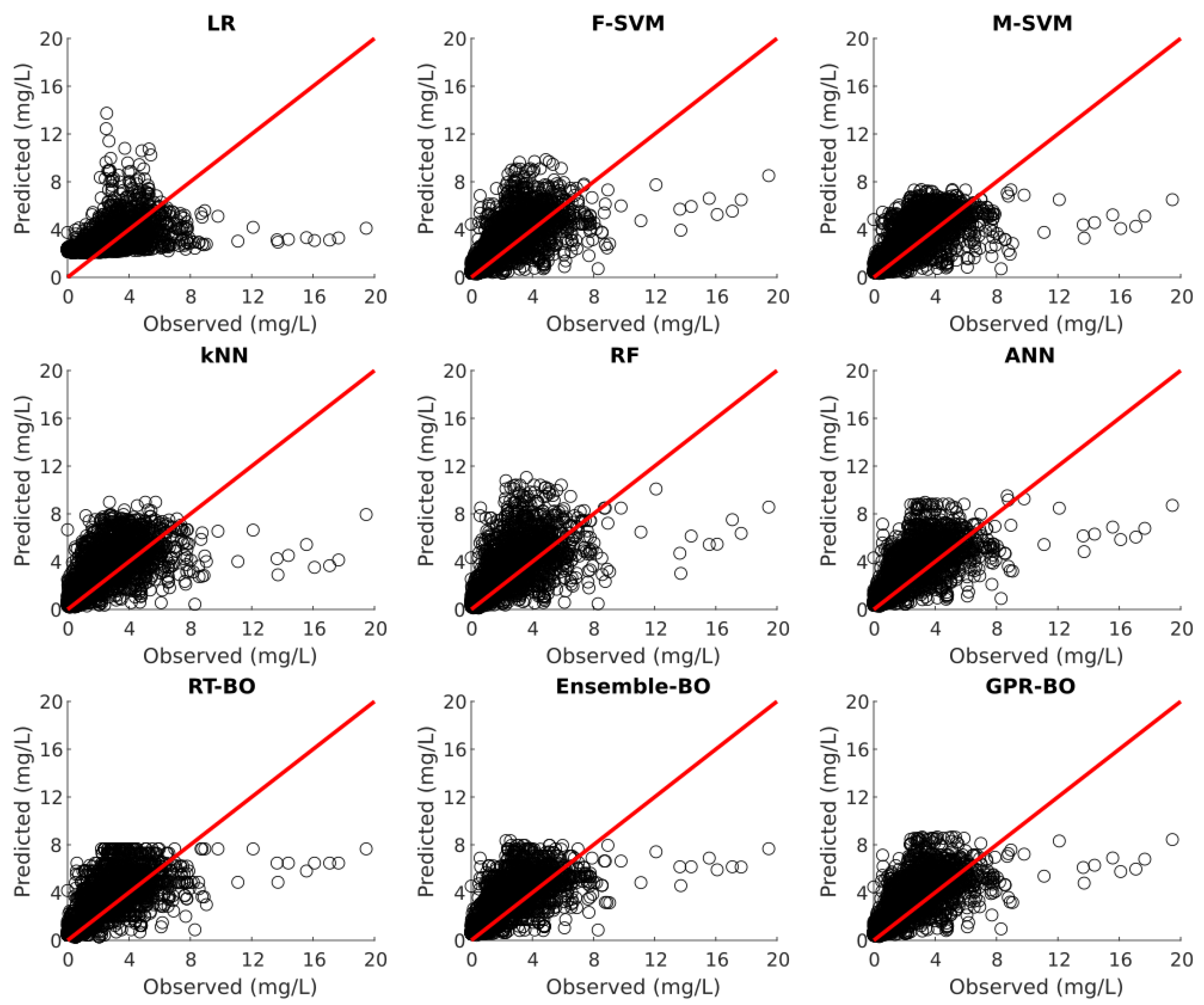
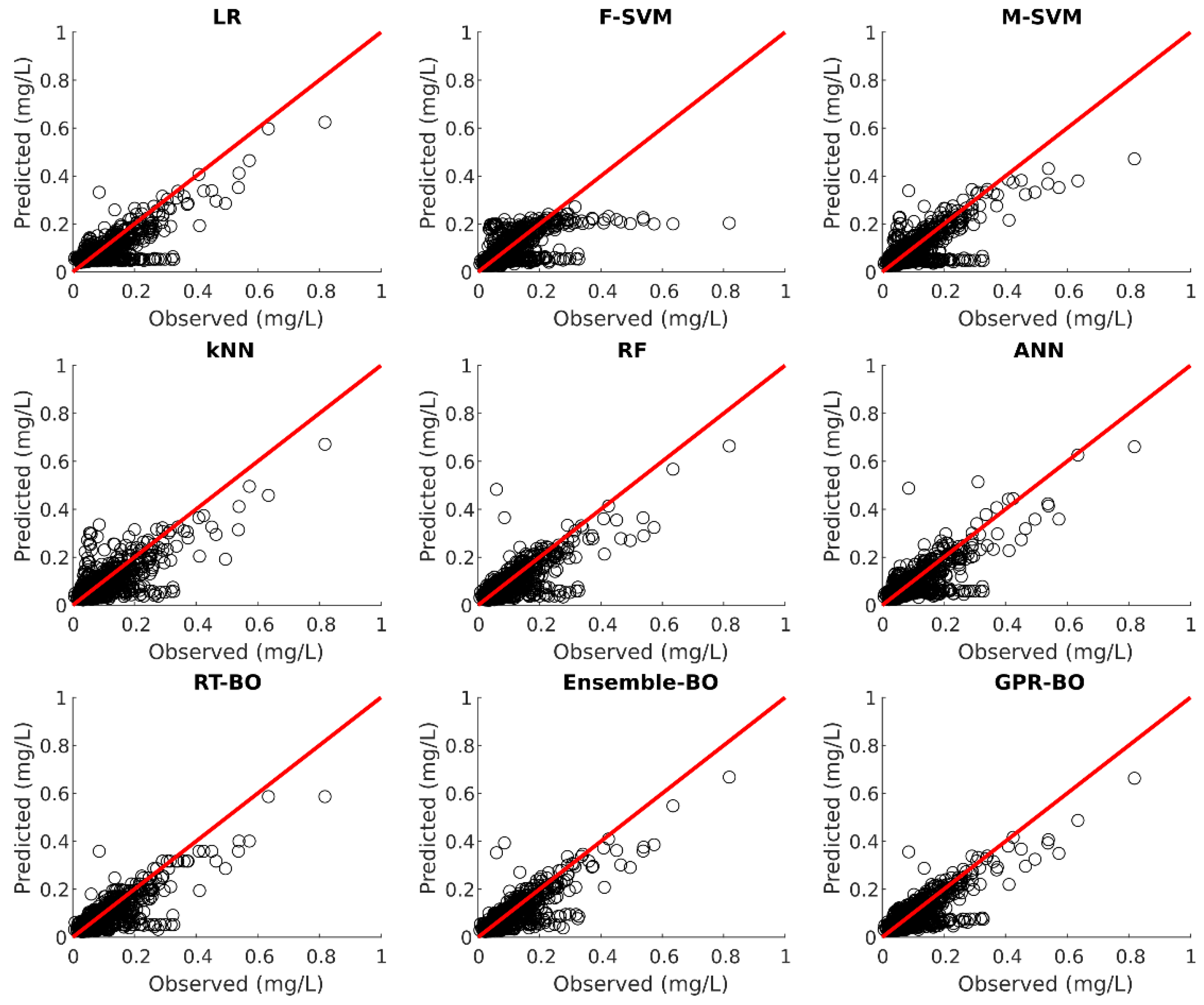
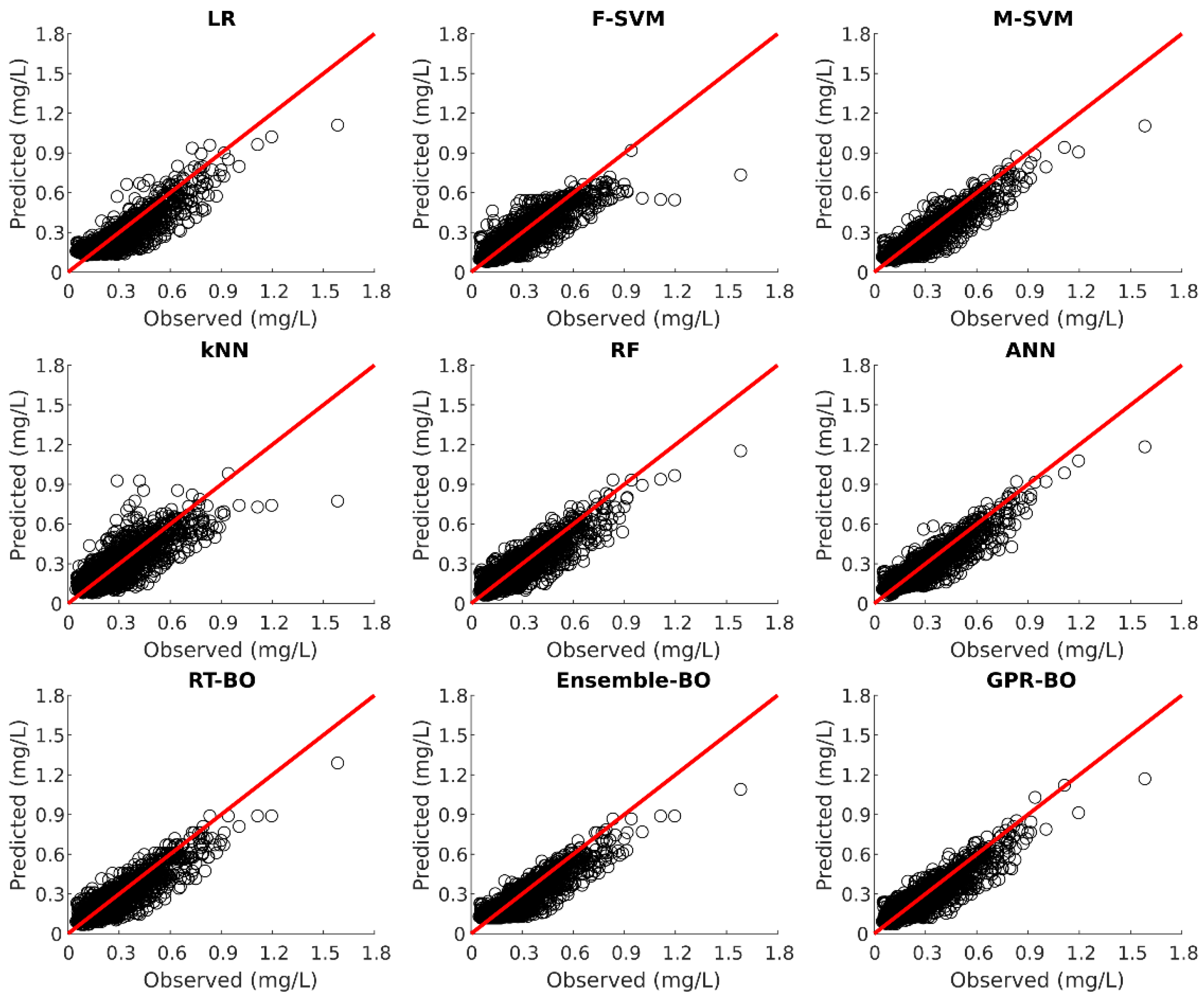
Model testing was carried out on 30% of the unseen test dataset after the model development.

Table 3. Comparison of $R^2$, RMSE, and MAE using different ML algorithms for nitrate prediction on test dataset.

Watershed	Parameter	LR	F-SVM	M-SVM	kNN	RF	ANN	RT-BO	Ensemble-BO	GPR-BO
Cuyahoga	$R^2$	0.404	0.751	0.745	0.690	0.689	0.754	0.745	0.749	0.752
	RMSE	1.0083	0.6748	0.6873	0.7300	0.7290	0.6670	0.6749	0.6702	0.6688
	MAE	0.7806	0.4836	0.4839	0.5360	0.5360	0.4860	0.4933	0.4900	0.4886
Grand River	$R^2$	0.039	0.152	0.188	0.023	0.079	0.093	0.214	0.173	0.145
	RMSE	0.3592	0.3479	0.3446	0.3840	0.3930	0.3740	0.3236	0.3335	0.3433
	MAE	0.2475	0.2334	0.2287	0.2740	0.2710	0.2570	0.2263	0.2345	0.2415
Maumee	$R^2$	0.160	0.463	0.462	0.282	0.387	0.479	0.466	0.470	0.477
	RMSE	2.5797	2.0970	2.0362	2.5140	2.4870	2.1780	2.2078	2.1863	2.1726
	MAE	2.1279	1.5809	1.5620	1.9500	1.8470	1.6880	1.7092	1.6886	1.6815
Raisin	$R^2$	0.251	0.466	0.476	0.409	0.406	0.485	0.468	0.485	0.482
	RMSE	1.8689	1.6611	1.5797	1.8310	1.9320	1.7130	1.7328	1.6797	1.7082
	MAE	1.4777	1.1395	1.0997	1.3080	1.3250	1.2310	1.2558	1.2159	1.2280
Sandusky	$R^2$	0.147	0.544	0.492	0.351	0.431	0.544	0.533	0.5395	0.542
	RMSE	2.6995	1.9639	2.0125	2.5060	2.5390	2.1590	2.1973	2.1850	2.1553
	MAE	2.1899	1.4242	1.4762	1.8670	1.8320	1.6340	1.6615	1.6662	1.6367

illustrates the fitting statistics of different ML models for nitrate concentration prediction on the test dataset. Figure 2, Figure 3, Figure 4, Figure 5 and Figure 6 show the observed versus predicted daily nitrate concentration using different ML models for the Cuyahoga, Grand, Maumee, Raisin, and Sandusky, respectively.

For the urban Cuyahoga watershed, F-SVM, M-SVM, ANN, RT-BO, ensemble-BO, and GPR-BO performed reasonably well in predicting the daily nitrate concentration for the test data. Among these models, ANN performs better than other ML models with $R^2$ of 0.754 and RMSE of 0.6670 $\mathrm{mg}/\mathrm{L}$. Regarding MAE, F-SVM outperforms other ML models with the value of 0.4836 $\mathrm{mg}/\mathrm{L}$. In urban watersheds, nitrate inputs mainly originate from wastewater treatment plants, urban runoff, and other periodic activities. This regular and predictable nature of nitrate concentrations in urban watersheds might be the reason for fairly accurate modeling of nitrate concentration with the streamflow and month of the year as independent variables [34].

On the contrary, for the forested Grand watershed, all the ML models showed mediocre performance with RT-BO being the best performing model $R^2$ of 0.214, RMSE of 0.3236 $\mathrm{mg}/\mathrm{L}$, and MAE of 0.2263 $\mathrm{mg}/\mathrm{L}$. For the agriculture-dominated watersheds of Maumee, Raisin and Sandusky, F-SVM, M-SVM, ANN, RT-BO, ensemble-BO, and GPR-BO again showed acceptable performance, which is lower than that of the Cuyahoga but better than the Grand. For the agricultural watersheds of Maumee and Raisin, ANN is the best performing model regarding the $R^2$ and M-SVM is the best performing model regarding RMSE and MAE. Likewise, for the agricultural Sandusky watershed, F-SVM was the best performing model with $R^2$ of 0.544, RMSE of 1.9639 $\mathrm{mg}/\mathrm{L}$, and MAE of 1.4242 $\mathrm{mg}/\mathrm{L}$.

The value for test statistics is similar for the training as well as the test set. Hence, the developed ML models can predict nitrate concentration without severely underfitting or overfitting the training dataset employing streamflow and month of the year as independent variables.

3.3. Relative Performance of ML Algorithms to Predict Phosphorus Concentration

3.3.1. Model Development

During the model development for the total phosphorus prediction, Bayesian optimized RT, ensemble, and GPR models were also run for 30 iterations. The convergence of objective function in the iterative process is illustrated in Figure 7. For the Cuyahoga watershed, ensemble converged to the minimum objective of 0.01485 after $29\mathrm{th}$ iteration. Hence, BO is more effective in improving ensemble compared to RT and GPR for the Cuyahoga watershed. Likewise, BO is more effective in improving ensemble compared to RT and GPR for Raisin (0.00559) and Sandusky (0.00365). On the contrary, BO is more effective in improving GPR compared to RT and Ensemble for Grand (0.00165) and Maumee (0.00362). The result of Bayesian optimized hyperparameters in RT, ensemble, and GPR models for phosphorus prediction is illustrated in

Table 4. Result of Bayesian optimized hyperparameters in RT, ensemble, and GPR models for phosphorus prediction.

Algorithm	Parameter	Cuyahoga	Grand	Maumee	Raisin	Sandusky
RT	Minimum leaf size	45	14	19	22	18
Ensemble	Ensemble method	Bag	Bag	LSBoost	LSBoost	Bag
	Minimum leaf size	23	4	3	9	8
	Number of learners	465	119	12	17	11
	Learning rate	-	-	0.26808	0.24101	-
	Number of predictors	3	3	3	3	3
GPR	Sigma	0.067662	0.02207	0.56943	1.0875	0.00010808
	Basis function	Constant	Linear	Linear	Constant	Constant
	Kernel function	Nonisotropic Exponential	Isotropic Exponential	Nonisotropic Exponential	Nonisotropic Exponential	Nonisotropic Exponential
	Kernel scale	418.2057	335.4861	96,562.4233	22,084.4674	25,385.3054
	Standardize	TRUE	TRUE	FALSE	FALSE	TRUE

.

Table 5. Comparison of $R^2$, RMSE, and MAE using different ML algorithms for phosphorus prediction on training dataset.

Watershed	Parameter	LR	F-SVM	M-SVM	kNN	RF	ANN	RT-BO	Ensemble-BO	GPR-BO
Cuyahoga	$R^2$	0.43	0.38	0.50	0.47	0.51	0.53	0.55	0.58	0.56
	RMSE	0.1419	0.1475	0.1327	0.1360	0.1310	0.1290	0.1258	0.1219	0.1237
	MAE	0.0885	0.0785	0.0740	0.0880	0.0830	0.0790	0.0801	0.0772	0.0782
Grand River	$R^2$	0.79	0.48	0.66	0.74	0.80	0.78	0.78	0.81	0.81
	RMSE	0.0428	0.0673	0.0544	0.0470	0.0420	0.0430	0.0431	0.0410	0.0406
	MAE	0.0219	0.0228	0.0201	0.0220	0.0180	0.0190	0.0193	0.0175	0.0178
Maumee	$R^2$	0.82	0.74	0.80	0.72	0.85	0.86	0.83	0.85	0.86
	RMSE	0.0676	0.0804	0.0700	0.0840	0.0620	0.0590	0.0646	0.0615	0.0602
	MAE	0.0466	0.0421	0.0400	0.0520	0.0410	0.0390	0.0417	0.0407	0.0386
Raisin	$R^2$	0.50	0.48	0.54	0.47	0.55	0.57	0.56	0.59	0.59
	RMSE	0.0825	0.0841	0.0789	0.0840	0.0780	0.0770	0.0773	0.0748	0.0748
	MAE	0.0448	0.0370	0.0359	0.0440	0.0400	0.0380	0.0395	0.0376	0.0368
Sandusky	$R^2$	0.85	0.77	0.86	0.82	0.88	0.88	0.87	0.89	0.88
	RMSE	0.0702	0.0851	0.0679	0.0760	0.0630	0.0610	0.0634	0.0604	0.0620
	MAE	0.0446	0.0377	0.0337	0.0440	0.0350	0.0330	0.0355	0.0336	0.0344

illustrates the fitting statistics of different ML models for phosphorus prediction on the training dataset. A comparison of statistical indicators shows that $R^2$, RMSE, and MAE, may follow a different trend. For the urban Cuyahoga watershed, M-SVM, RF, ANN, RT-BO, ensemble-BO, and GPR-BO showed acceptable performance in explaining the variance of phosphorus concentration. Among these models, ensemble-BO performs better than other ML models with $R^2$ of 0.58 and RMSE of 0.1219 $\mathrm{mg}/\mathrm{L}$ for the training set. Likewise, GPR-BO ranks second with $R^2$ of 0.56 and RMSE of 0.1237 $\mathrm{mg}/\mathrm{L}$. Regarding MAE, M-SVM is the best performing model with MAE of 0.0740 $\mathrm{mg}/\mathrm{L}$.

Likewise, for the forested Grand watershed, LR, kNN, RF, ANN, RT-BO, ensemble-BO, and GPR-BO performed well in explaining the variance of phosphorus concentration with total suspended solids, streamflow, and month of the year as independent variables. Among these models, GPR-BO performed better than other ML models with $R^2$ of 0.81 and RMSE of 0.0406 $\mathrm{mg}/\mathrm{L}$ for the training set. Regarding MAE, ensemble-BO is the best performing model with MAE of 0.0175 $\mathrm{mg}/\mathrm{L}$. Similarly, for the agricultural watersheds (Maumee and Sandusky), LR, M-SVM, kNN, RF, ANN, RT-BO, ensemble-BO, and GPR-BO also performed exceptionally well in explaining the variance of phosphorus concentration. GPR-BO was the best performing model for Maumee regarding $R^2$ and MAE and ensemble-BO was the best performing model for Sandusky regarding $R^2$ and RMSE. For the agricultural Raisin watershed, LR, M-SVM, RF, ANN, RT-BO, ensemble-BO, and GPR-BO showed acceptable performance in explaining the variance of phosphorus concentration. Among these models, ensemble-BO and GPR-BO performed similarly with $R^2$ of 0.59 and RMSE of 0.0748 $\mathrm{mg}/\mathrm{L}$ for the training set. Regarding MAE, M-SVM was the best performing model with MAE of 0.0359 $\mathrm{mg}/\mathrm{L}$.

The model predictability of ML models was significantly high in predicting phosphorus concentration for the forested and agricultural watersheds. It was also observed that the model predictability of traditional LR model was comparable to that of the ML models in predicting the phosphorus concentration for the training dataset.

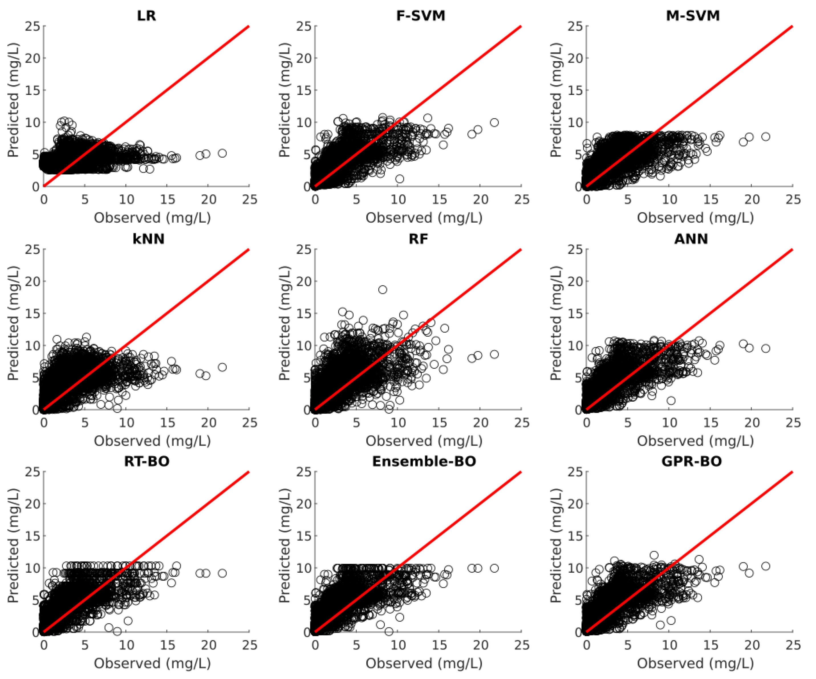
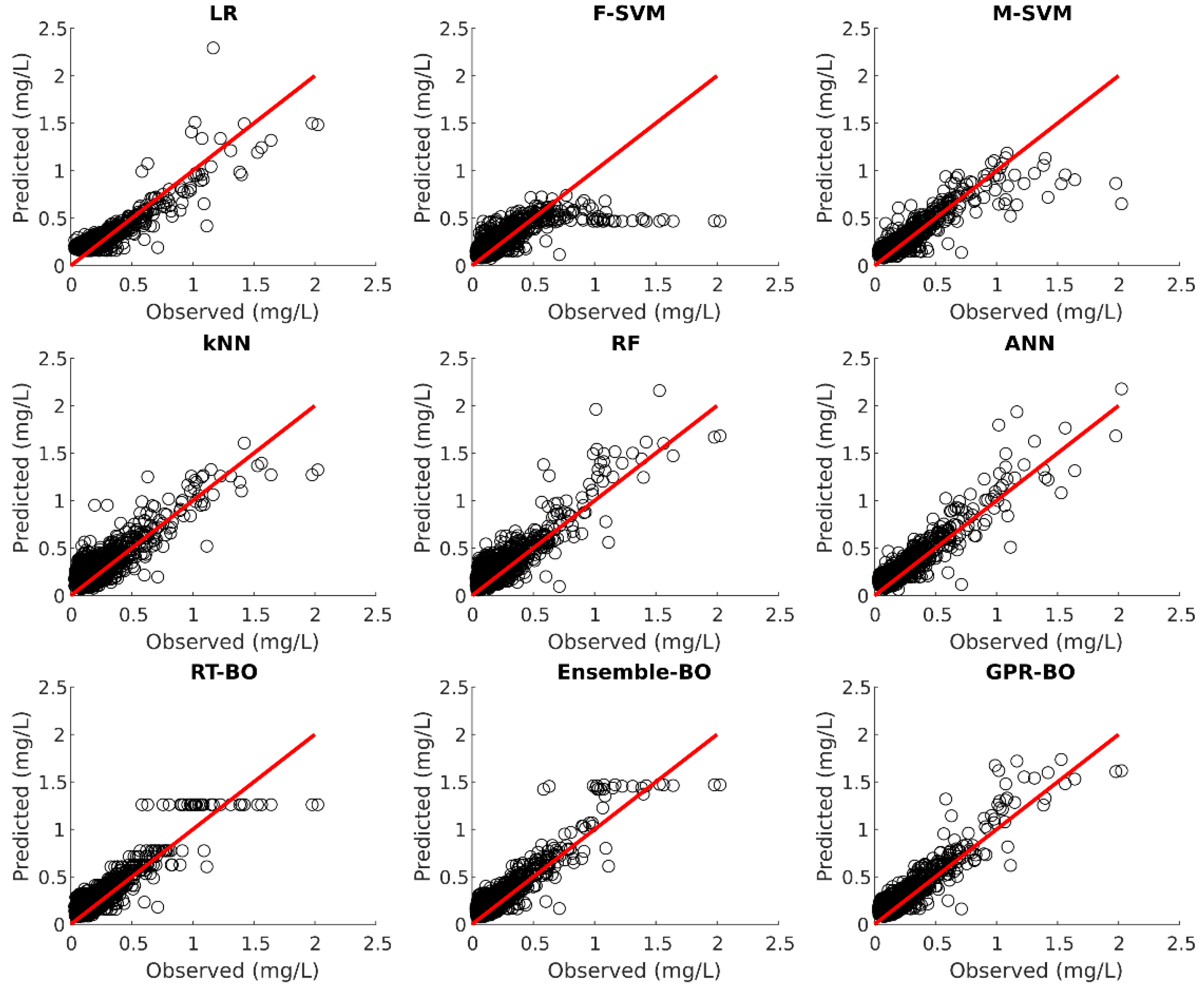
3.3.2. Model Testing

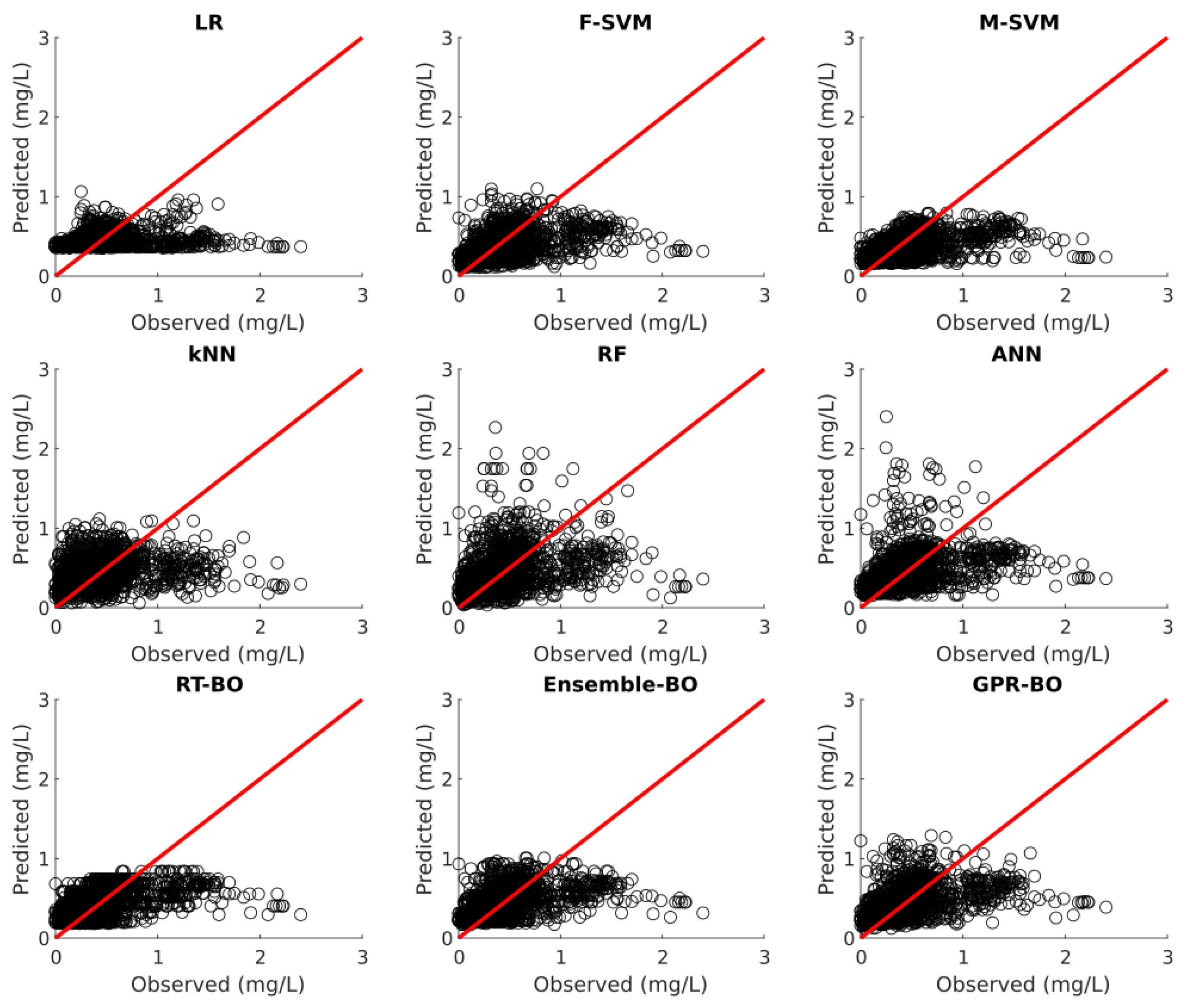
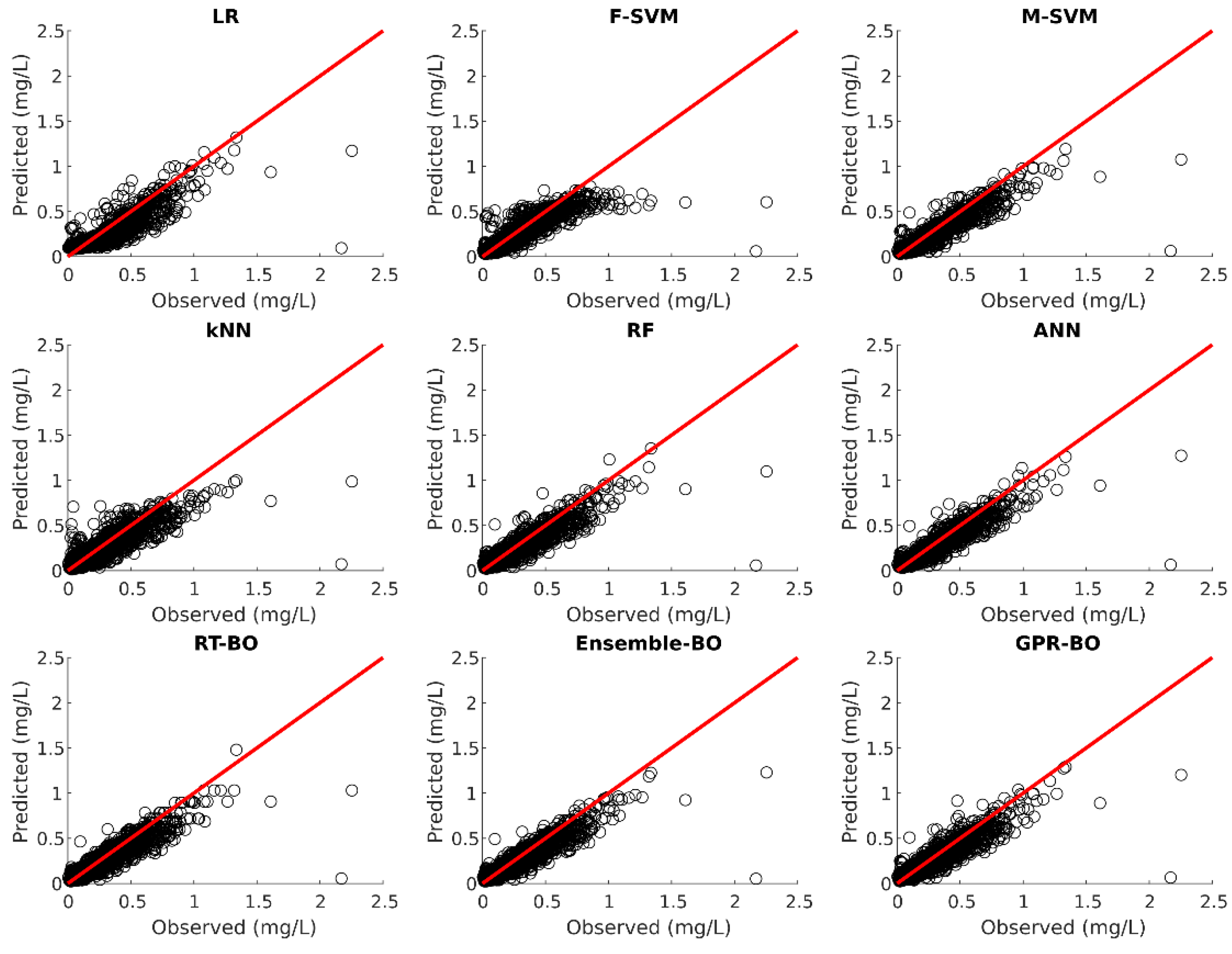
Model testing is carried out on the 30% of the unseen test dataset after the model development.

Table 6. Comparison of $R^2$, RMSE, and MAE using different ML algorithms for phosphorus prediction on test dataset.

Watershed	Parameter	LR	F-SVM	M-SVM	kNN	RF	ANN	RT-BO	Ensemble-BO	GPR-BO
Cuyahoga	$R^2$	0.800	0.574	0.778	0.720	0.754	0.829	0.778	0.808	0.820
	RMSE	0.1007	0.1013	0.0766	0.1000	0.1034	0.0901	0.0975	0.0941	0.0926
	MAE	0.0873	0.0618	0.0511	0.0765	0.0787	0.0737	0.0770	0.0745	0.0746
Grand River	$R^2$	0.665	0.483	0.633	0.590	0.676	0.665	0.720	0.733	0.718
	RMSE	0.0414	0.0505	0.0429	0.0294	0.0264	0.0264	0.0381	0.0369	0.0375
	MAE	0.0251	0.0266	0.0240	0.0111	0.0093	0.0097	0.0215	0.0204	0.0216
Maumee	$R^2$	0.800	0.800	0.850	0.708	0.812	0.846	0.822	0.838	0.842
	RMSE	0.0640	0.0629	0.0568	0.0743	0.0603	0.0556	0.0592	0.0587	0.0563
	MAE	0.0466	0.0414	0.0390	0.0514	0.0427	0.0390	0.0417	0.0407	0.0391
Raisin	$R^2$	0.652	0.688	0.762	0.561	0.618	0.680	0.671	0.709	0.697
	RMSE	0.0572	0.0507	0.0459	0.0578	0.0539	0.0505	0.0504	0.0488	0.0487
	MAE	0.0389	0.0264	0.0236	0.0341	0.0311	0.0308	0.0296	0.0285	0.0283
Sandusky	$R^2$	0.817	0.816	0.876	0.808	0.857	0.877	0.868	0.878	0.865
	RMSE	0.0895	0.0885	0.0752	0.0879	0.0774	0.0729	0.0758	0.0737	0.0751
	MAE	0.0567	0.0426	0.0395	0.0493	0.0416	0.0391	0.0403	0.0394	0.0399

illustrates the fitting statistics of different ML models for phosphorus prediction on the test dataset. Figure 8, Figure 9, Figure 10, Figure 11 and Figure 12 show the observed versus predicted daily phosphorus concentration using different ML models for the Cuyahoga, Grand, Maumee, Raisin, and Sandusky, respectively.

For the urban Cuyahoga watershed, LR, M-SVM, RF, ANN, RT-BO, Ensemble-BO, and GPR-BO performed reasonably well in predicting the daily phosphorus concentration for the test data. Among these models, ANN outperformed other models regarding $R^2$ (0.829) and M-SVM outperforms other models with RMSE of 0.0766 $\mathrm{mg}/\mathrm{L}$ and MAE of 0.0511 $\mathrm{mg}/\mathrm{L}$ for the test set. The developed ML models performed exceptionally well in test data in comparison to the training data. Hence, it could be concluded that the ML models for the Cuyahoga was underfitting the training dataset.

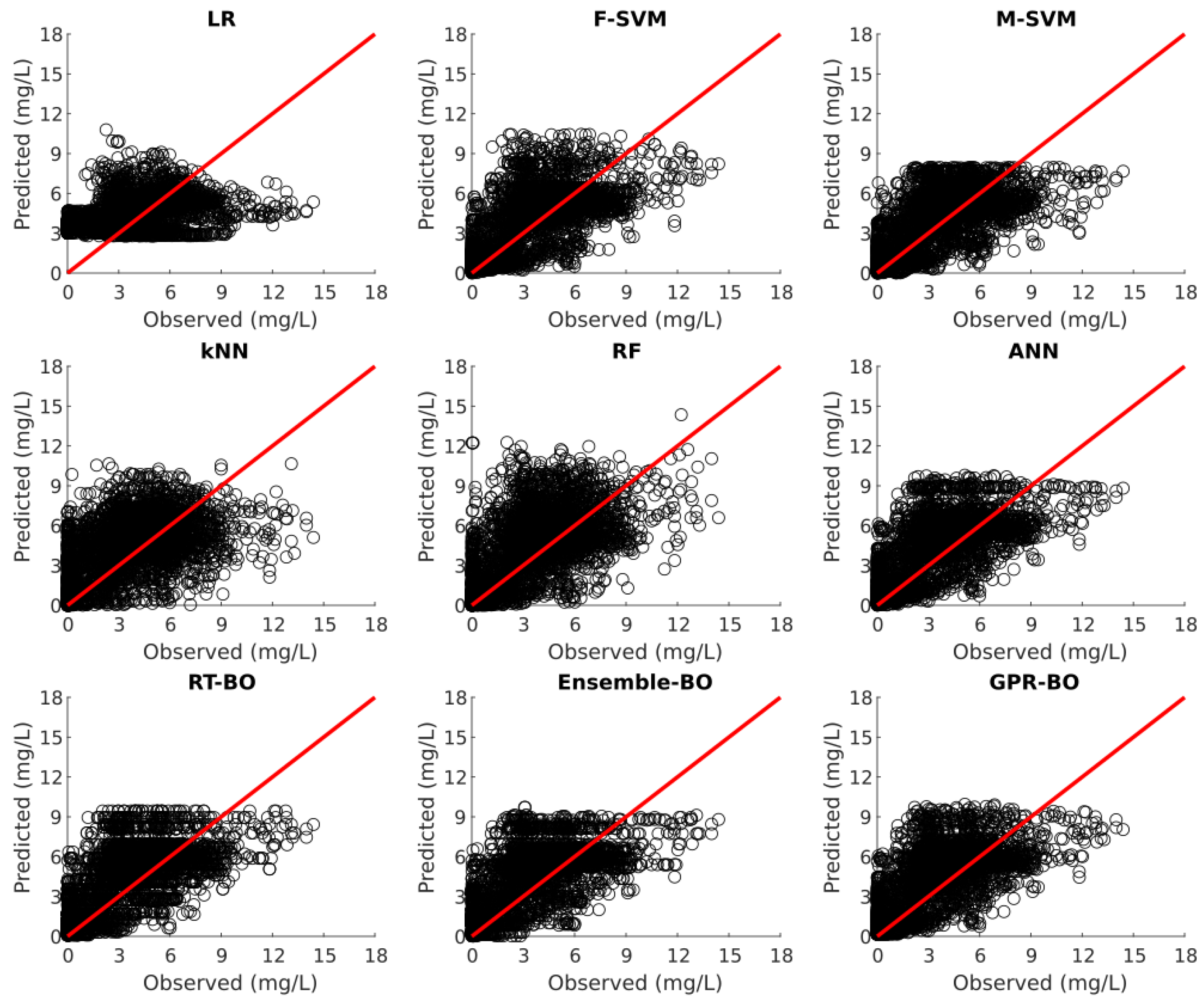
Likewise, for the forested Grand watershed, LR, M-SVM, RF, ANN, RT-BO, Ensemble-BO, and GPR-BO performed reasonably well in predicting the daily phosphorus concentration with total suspended solids, streamflow, and month of the year as independent variables. Among these models, ensemble-BO outperformed other models regarding $R^2$ (0.733) and RF outperformed other models with RMSE of 0.0264 $\mathrm{mg}/\mathrm{L}$ and MAE of 0.0093 $\mathrm{mg}/\mathrm{L}$ for the test set. Similarly, for the agricultural watersheds of Maumee and Sandusky, all ML models performed exceptionally well in predicting the daily phosphorus concentration. For Maumee watershed, M-SVM outperformed other models regarding $R^2$ (0.850) and ANN outperformed other models with RMSE of 0.0556 $\mathrm{mg}/\mathrm{L}$. Regarding MAE, both M-SVM and ANN have the minimum value of 0.0390 $\mathrm{mg}/\mathrm{L}$ for the Maumee watershed. For Sandusky watershed, ensemble-BO performed better than other ML models regarding $R^2$ (0.878) and ANN performed better than other ML models with RMSE of 0.0729 $\mathrm{mg}/\mathrm{L}$ and MAE of 0.0391 $\mathrm{mg}/\mathrm{L}$. For the agricultural Raisin watershed, all ML models except kNN performed reasonably well in predicting the daily phosphorus concentration for the test dataset. Among these models, M-SVM outperformed all other models with $R^2$ of 0.762, RMSE of 0.0459 $\mathrm{mg}/\mathrm{L}$, and MAE of 0.0236 $\mathrm{mg}/\mathrm{L}$. For the agricultural and forested watershed, value for test statistics was similar for the training as well as test set while predicting the daily phosphorus concentration. Hence, the developed ML models could accurately predict daily phosphorus concentration without severely underfitting or overfitting the training dataset for the agricultural and forested watershed.

Suspended solids are derived from nonpoint sources from agricultural lands and construction sites in the urban areas. Most of the total phosphorus is particulate phosphorus attached to suspended solid particles. In agricultural and forested watershed, increased streamflow can increase soil erosion which can elevate the particulate phosphorus concentration in water column. Hence, in predicting phosphorus concentration, the model predictability is better for agricultural and forested watersheds. On the contrary, in urban watershed, phosphorus inputs mainly originate from point sources such as wastewater treatment plants. Hence, in predicting phosphorus concentration, the model predictability is a bit deteriorated.

3.4. Discussion

Various ML models, namely, MLP, radial basis function (RBF), general regression neural network (GRNN), kNN, RF, MLR, evolutionary polynomial regression (EPR), naïve Bayes model (NBM) and many more have been employed to predict groundwater as well as surface water nutrient concentration. In one such study, Al-Mahallawi et al. [6] found that MLP ($R^2=0.955$ and error = 8.4322) with six input nodes and 4 hidden nodes outperformed RBF, GRNN, and other linear networks to predict groundwater nitrate concentration in the Gaza Strip Aquifer. In another study to model groundwater nitrate contamination at the African continent scale, Ouedraogo et al. [8] concluded that the predictive power of RF ($R^2=0.97$) was more than the MLR ($R^2=0.64$).

Furthermore, Markus et al. [35] compared the performance of ANN, EPR, and NBM to predict weekly fluctuations of nitrate concentration in a small agricultural watershed in Illinois. They found that the ANN (RMSE = 0.935) with two hidden nodes was the most accurate. In a more recent study, Li et al. [3] analyzed the performance of MLP, kNN, RF, and reduced error pruning tree (REPTree) to predict nitrate concentration and estimate nutrient loading in different types of watersheds. They concluded that the REPTree was the best performing model with $R^2$ ranging from 0.61 to 0.85. The classification tree methods (REPTree and RF) performed better than the cluster methods (MLP and kNN) for agricultural and forested watersheds. Shen et al. [36] presented a novel geo-dataset to estimate and map the nitrate and phosphorus concentrations in streams and rivers with models built using a RF. The developed model had $R^2$ of 0.66 on average.

The model performance is not only determined by the model complexity but also by the land-use practices in the watershed. In comparison to the published literature, the developed ML models are more accurate in predicting nitrate concentration for the urban and agricultural watershed. The ANN is the best performing model with $R^2$ ranging from 0.479 to 0.745. Likewise, in comparison to the published literature, the developed ML models are more accurate in predicting phosphorus concentration for all type of watersheds. The ensemble-BO is the best performing model with $R^2$ ranging from 0.709 to 0.878. As a limited number of independent variables are employed in the study, these methods can be applied to predict nutrient concentrations with limited data, which increases the applicability of the developed models. Hence, the ML model must be selected considering the land-use practice alongside algorithmic methods to accurately predict nutrient concentration.

4. Conclusions

In this study, the performance of nine different ML algorithms (LR, F-SVM, M-SVM, kNN, RF, ANN, RT-BO, ensemble-BO, and GPR-BO) was evaluated to predict nitrate and total phosphorus concentration for different types of watersheds. Initially, the C–Q relationship was analyzed for each watershed to understand the impact of watershed type on the prediction of nutrient concentration. While the nitrate concentration diluted with the increasing streamflow in the urban Cuyahoga watershed, it increased with the streamflow in agricultural and forested watersheds. Similarly, the total phosphorus concentration increased with the streamflow irrespective of the type of watershed.

For nitrate concentration prediction, the land-use distribution affected the model performance for all methods. In urban watersheds, the regular and predictable nature of nitrate concentration results in more accurate modeling with the streamflow and month of the year as independent variables. Likewise, ML models were more accurate in predicting nitrate concentration for the agricultural watershed (Maumee, Raisin, and Sandusky) in comparison to the forested Grand watershed. The ANN outperformed other ML models regarding the $R^2$ for the urban and agricultural watersheds. On the contrary, for the forested Grand watershed, RT-BO outperformed other ML models. Likewise, the Bayesian optimized RT, ensemble, and GPR consistently yielded good performance for all type of watersheds.

In agricultural and forested watersheds, increased streamflow could increase soil erosion which could elevate the particulate phosphorus concentration in the water column. Hence, in predicting phosphorus concentration, the model predictability was better for agricultural and forested watersheds with the streamflow, total suspended solids, and month of the year as independent variables. On the contrary, in an urban watershed, phosphorus inputs mainly originate from point sources such as wastewater treatment plants. Hence, in predicting phosphorus concentration, the model predictability was a bit deteriorated. For the urban Cuyahoga watershed, the developed ML models were underfitting the training dataset and the ANN appeared to outperform other ML models regarding the $R^2$ for the test data. On the contrary, ensemble-BO and M-SVM outperformed other ML models in predicting total phosphorus concentration for the agricultural and forested watershed.

In comparison to the published literature, the developed ML models were more accurate in predicting nitrate concentration for the urban and agricultural watershed. The ANN was the best performing model with $R^2$ ranging from 0.479 to 0.745. Likewise, in comparison to the published literature, the developed ML models were more accurate in predicting phosphorus concentration for all types of watersheds. The ensemble-BO was the best performing model with $R^2$ ranging from 0.709 to 0.878. As a limited number of independent variables were employed in the study, these methods could be applied to predict nutrient concentrations with limited data, which increased the applicability of the developed models. Regarding the shortcoming of the developed ML models, the model predictability for nitrate concentration in the forested Grand watershed was greatly diminished. Hence, further study is required in this regard to identify additional independent variables to improve the model predictability of ML algorithms.

References

- Boyd, C.E. Water Quality: An Introduction; Springer Nature: Cham, Switzerland, 2019. [Google Scholar]
- Goel, P.K. Water Pollution: Causes, Effects and Control; New Age International: New Delhi, India, 2006. [Google Scholar]
- Li, S.; Bhattarai, R.; Cooke, R.A.; Verma, S.; Huang, X.; Markus, M.; Christianson, L. Relative performance of different data mining techniques for nitrate concentration and load estimation in different type of watersheds. Environ. Pollut. 2020, 263, 114618. [Google Scholar] [CrossRef] [PubMed]
- Ahmed, A.N.; Othman, F.B.; Afan, H.A.; Ibrahim, R.K.; Fai, C.M.; Hossain, M.S.; Ehteram, M.; Elshafie, A. Machine learning methods for better water quality prediction. J. Hydrol. 2019, 578, 124084. [Google Scholar] [CrossRef]
- Heuvelmans, G.; Muys, B.; Feyen, J. Regionalisation of the parameters of a hydrological model: Comparison of linear regression models with artificial neural nets. J. Hydrol. 2006, 319, 245–265. [Google Scholar] [CrossRef]
- Al-Mahallawi, K.; Mania, J.; Hani, A.; Shahrour, I. Using of neural networks for the prediction of nitrate groundwater contamination in rural and agricultural areas. Environ. Earth Sci. 2012, 65, 917–928. [Google Scholar] [CrossRef]
- Modaresi, F.; Araghinejad, S. A comparative assessment of support vector machines, probabilistic neural networks, and K-nearest neighbor algorithms for water quality classification. Water Resour. Manag. 2014, 28, 4095–4111. [Google Scholar] [CrossRef]
- Ouedraogo, I.; Defourny, P.; Vanclooster, M. Application of random forest regression and comparison of its performance to multiple linear regression in modeling groundwater nitrate concentration at the African continent scale. Hydrogeol. J. 2019, 27, 1081–1098. [Google Scholar] [CrossRef]
- Bindra, H.; Jain, R.; Singh, G.; Garg, B. Application of Classification Techniques for Prediction of Water Quality of 17 Selected Indian Rivers. In Data Management, Analytics and Innovation; Springer: Singapore, 2019; pp. 237–247. [Google Scholar]
- Nieto, P.G.; García-Gonzalo, E.; Fernández, J.A.; Muñiz, C.D. Water eutrophication assessment relied on various machine learning techniques: A case study in the Englishmen Lake (Northern Spain). Ecol. Model. 2019, 404, 91–102. [Google Scholar] [CrossRef]
- Karamoutsou, L.; Psilovikos, A. Modeling of Dissolved Oxygen concentration using a Deep Neural Network approach in Lake Kastoria, Greece. Eur. Water 2020, 71/72, 3–14. [Google Scholar]
- Anctil, F.; Filion, M.; Tournebize, J. A neural network experiment on the simulation of daily nitrate-nitrogen and suspended sediment fluxes from a small agricultural catchment. Ecol. Model. 2009, 220, 879–887. [Google Scholar] [CrossRef] [Green Version]
- Yu, C.Y.; Northcott, W.J.; Mitchell, J.K.; McIsaac, G. Development of an artificial neural network model for hydrologic and water quality modeling of agricultural watersheds. In Proceedings of the 2001 ASAE Annual Meeting, Sacramento, CA, USA, 28 July–1 August 2001; American Society of Agricultural and Biological Engineers: St. Joseph, MI, USA, 1998. [Google Scholar]
- Chau, K. A review on the integration of artificial intelligence into coastal modeling. J. Environ. Manag. 2006, 80, 47–57. [Google Scholar] [CrossRef] [PubMed] [Green Version]
- Najah, A.; Elshafie, A.; Karim, O.A.; Jaffar, O. Prediction of Johor River water quality parameters using artificial neural networks. Eur. J. Sci. Res. 2009, 28, 422–435. [Google Scholar]
- Faruk, D.Ö. A hybrid neural network and ARIMA model for water quality time series prediction. Eng. Appl. Artif. Intell. 2010, 23, 586–594. [Google Scholar] [CrossRef]
- Palani, S.; Liong, S.Y.; Tkalich, P. An ANN application for water quality forecasting. Mar. Pollut. Bull. 2008, 56, 1586–1597. [Google Scholar] [CrossRef] [PubMed]
- Poor, C.J.; Ullman, J.L. Using regression tree analysis to improve predictions of low-flow nitrate and chloride in Willamette River Basin watersheds. Environ. Manag. 2010, 46, 771–780. [Google Scholar] [CrossRef] [PubMed]
- Zare, M.; Pourghasemi, H.R.; Vafakhah, M.; Pradhan, B. Landslide susceptibility mapping at Vaz Watershed (Iran) using an artificial neural network model: A comparison between multilayer perceptron (MLP) and radial basic function (RBF) algorithms. Arab. J. Geosci. 2013, 6, 2873–2888. [Google Scholar] [CrossRef]
- Castillo, E.; Corrales, D.C.; Lasso, E.; Ledezma, A.; Corrales, J.C. Data processing for a water quality detection system on Colombian Rio Piedras Basin. In Proceedings of the International Conference on Computational Science and Its Applications, Beijing, China, 4–7 July 2016; Springer: Cham, Switzerland, 2016. [Google Scholar]
- Gonzalez, H.; Morell, C.; Ferri, F.J. Improving nearest neighbor based multi-target prediction through metric learning. In Proceedings of the Iberoamerican Congress on Pattern Recognition, Lima, Peru, 8–11 November 2016; Springer: Cham, Switzerland, 2016. [Google Scholar]
- Sattari, M.T.; Joudi, A.R.; Kusiak, A. Estimation of Water Quality Parameters with Data-Driven Model. J. Am. Water Work. Assoc. 2016, 108, E232–E239. [Google Scholar] [CrossRef] [Green Version]
- Towler, E.; Rajagopalan, B.; Seidel, C.; Summers, R.S. Simulating ensembles of source water quality using a K-nearest neighbor resampling approach. Environ. Sci. Technol. 2009, 43, 1407–1411. [Google Scholar] [CrossRef]
- Li, S.; Bhattarai, R.; Wang, L.; Cooke, R.A.; Ma, F.; Kalita, P.K. Assessment of water quality in Little Vermillion River watershed using principal component and nearest neighbor analyses. Water Sci. Technol. Water Supply 2015, 15, 327–338. [Google Scholar] [CrossRef]
- Tharwat, A.; Mahdi, H.; Elhoseny, M.; Hassanien, A.E. Recognizing human activity in mobile crowdsensing environment using optimized k-NN algorithm. Expert Syst. Appl. 2018, 107, 32–44. [Google Scholar] [CrossRef]
- National Center for Water Quality Research (NCWQR), Tributary Data Download. 2009. Available online: https://www.heidelberg.edu/tributary-data-download (accessed on 13 September 2021).
- The Math Works, Inc., MATLAB (Version 2020a) [Computer Software]. 2020. Available online: https://www.mathworks.com/ (accessed on 13 September 2021).
- Chen, C.H.; Huang, W.T.; Tan, T.H.; Chang, C.C.; Chang, Y.J. Using k-nearest neighbor classification to diagnose abnormal lung sounds. Sensors 2015, 15, 13132–13158. [Google Scholar] [CrossRef] [PubMed] [Green Version]
- Shevade, S.K.; Keerthi, S.S.; Bhattacharyya, C.; Murthy, K.R.K. Improvements to the SMO algorithm for SVM regression. IEEE Trans. Neural Netw. 2000, 11, 1188–1193. [Google Scholar] [CrossRef] [PubMed] [Green Version]
- Sameen, M.I.; Pradhan, B.; Lee, S. Self-learning random forests model for mapping groundwater yield in data-scarce areas. Nat. Resour. Res. 2019, 28, 757–775. [Google Scholar] [CrossRef]
- Walpole, R.E.; Myers, R.H.; Myers, S.L.; Ye, K. Probability and Statistics for Engineers and Scientists; Macmillan: New York, NY, USA, 1993; Volume 5. [Google Scholar]
- Duncan, J.M.; Welty, C.; Kemper, J.T.; Groffman, P.M.; Band, L.E. Dynamics of nitrate concentration-discharge patterns in an urban watershed. Water Resour. Res. 2017, 53, 7349–7365. [Google Scholar] [CrossRef]
- Charulatha, G.; Srinivasalu, S.; Maheswari, O.U.; Venugopal, T.; Giridharan, L. Evaluation of ground water quality contaminants using linear regression and artificial neural network models. Arab. J. Geosci. 2017, 10, 128. [Google Scholar] [CrossRef]
- Groffman, P.M.; Law, N.L.; Belt, K.T.; Band, L.E.; Fisher, G.T. Nitrogen fluxes and retention in urban watershed ecosystems. Ecosystems 2004, 7, 393–403. [Google Scholar] [CrossRef]
- Markus, M.; Hejazi, M.I.; Bajcsy, P.; Giustolisi, O.; Savic, D.A. Prediction of weekly nitrate-N fluctuations in a small agricultural watershed in Illinois. J. Hydroinform. 2010, 12, 251–261. [Google Scholar] [CrossRef]
- Shen, L.Q.; Amatulli, G.; Sethi, T.; Raymond, P.; Domisch, S. Estimating nitrogen and phosphorus concentrations in streams and rivers, within a machine learning framework. Sci. Data 2020, 7, 161. [Google Scholar] [CrossRef] [PubMed]
Figure 1.
Objective in the iterative process of BO for nitrate prediction.
Figure 2.
Observed versus predicted daily nitrate concentration for the Cuyahoga watershed using different ML algorithms.
Figure 3.
Observed versus predicted daily nitrate concentration for the Grand watershed using different ML algorithms.
Figure 4.
Observed versus predicted daily nitrate concentration for Maumee using different ML algorithms.
Figure 5.
Observed versus predicted daily nitrate concentration for Raisin using different ML algorithms.
Figure 6.
Observed versus predicted daily nitrate concentration for Sandusky using different ML algorithms.
Figure 7.
Objective in the iterative process of BO for phosphorus prediction.
Figure 8.
Observed versus predicted daily phosphorus concentration for the Cuyahoga using different ML algorithms.
Figure 9.
Observed versus predicted daily phosphorus concentration for the Grand using different ML algorithms.
Figure 10.
Observed versus predicted daily phosphorus concentration for Maumee using different ML.
Figure 11.
Observed versus predicted daily phosphorus concentration for Raisin using different ML.
Figure 12.
Observed versus predicted daily phosphorus concentration for Sandusky using different ML algorithms.